An enhanced POSTA based on Nelder-Mead simplex search and quadratic interpolation

Abstract

State transition algorithm (STA) is a metaheuristic method for global optimization. Recently, a modified STA named parameter optimal state transition algorithm (POSTA) is proposed. In POSTA, the performance of expansion operator, rotation operator and axesion operator is optimized through a parameter selection mechanism. But due to the insufficient utilization of historical information, POSTA still suffers from slow convergence speed and low solution accuracy on specific problems. To make better use of the historical information, Nelder-Mead (NM) simplex search and quadratic interpolation (QI) are integrated into POSTA. The enhanced POSTA is tested against 14 benchmark functions with 20-D, 30-D and 50-D space. An experimental comparison with several competitive metaheuristic methods demonstrates the effectiveness of the proposed method.

1 Introduction

State transition algorithm (STA) [1, 2] is a novel metaheuristic method for global optimization and has been successfully applied in many fields [3, 4, 5]. The basic idea of STA is to regard a solution as a state. Therefore the update of a solution can be considered as a state transition. In STA, four state transformation operators are designed to generate candidate solutions, namely expansion operator, rotation operator, axesion operator and translation operator. Among these operators, expansion operator is used for global search, rotation operator is for local search, axesion operator is for single-dimensional search and translation operator is designed for heuristic search [6]. Designed for different functionality, the state transformation operators are iteratively invoked to generate promising solutions until terminal conditions are satisfied.

Recently, a modified STA named parameter optimal state transition algorithm (POSTA) [6] is proposed. Based on a statistical study, POSTA provides a parameter selection mechanism to select optimal parameters for expansion operator, rotation operator and axesion operator. As a result, POSTA has better solution accuracy and stronger global exploration ability than STA. However, the historical information in POSTA is not sufficiently utilized. During the whole search process, the insufficient utilization of historical information leads to a slow convergence speed. In POSTA, the historical information is utilized by the translation operator. When a better solution emerges, the translation operator searches along the line between the current solution and the last solution with a maximal length of $\beta$. Obviously, the historical information is not sufficiently utilized, only two historical solutions are considered and only a linear transformation is applied for utilization. This inefficiency leads to a relatively slow convergence speed. In the later stage of the search, the lack of utilizing historical information leads to a low solution accuracy. As a metaheuristic method, POSTA is efficient to globally explore the whole solution space and localize the promising areas. But when the promising areas are reached, the lack of using historical information leads to a low probability of generating better solutions. This inefficiency leads to a relatively low solution accuracy. The above discussion implies that due to the insufficient utilization of historical information, POSTA still suffers from slow convergence speed and low solution accuracy on specific problems.

To speed up the convergence during the whole search process, Nelder-Mead (NM) simplex search [7, 8] is introduced. NM simplex search is a classical direct search method with a fast convergence speed. For decades, combining NM simplex search with metaheuristic methods has been a popular way to speed up the convergence [9, 10]. But none of the existing combination strategies have seen NM simplex search as a way to utilize the historical information. In this paper, a new combination strategy is proposed by applying NM simplex search to make use of the historical information. In the proposed method, the NM simplex is used to store the historical information and the NM geometric transformations are applied to utilize the historical information. The NM simplex is a geometric figure consisting of $n+1$ vertices in n-dimensional space. Therefore, the NM simplex is able to store the information of $n+1$ historical solutions, which is more than the two historical solutions in translation operator. On the other hand, the NM geometric transformations consists of a sequence of distinct geometric transformations (reflection, contraction …), which are more comprehensive than the linear transformation in translation operator. Therefore, applying NM simplex search is feasible to utilize the historical information more sufficiently and speed up the convergence. To improve the solution accuracy in later stage of the search, a quadratic interpolation (QI) strategy is introduced. QI is a classical local search method and is widely used [11, 12, 13, 14]. In QI, three known points are used as the search agents to generate a quadratic curve. The generated curve is seen as an approximate shape of the target function. Therefore the extreme point of the quadratic function can be seen as an approximate optima of the target function. To make use of the historical information, three historical solutions are selected as the QI search agents to generate a new analytical solution with little computing cost. Therefore, QI is feasible to strengthen the exploitation capacity by utilizing historical information. By applying NM simplex search and QI in different stage of the search, the historical information of POSTA is utilized efficiently. Therefore, an enhanced POSTA based on NM simplex search and QI is proposed.

The main contributions of this paper can be summarized as follows: (1) A modified POSTA named the enhanced POSTA is proposed. (2) In the proposed method, the historical information is utilized more sufficiently to improve the performance. (3) The proposed method successfully combines the merits of the three distinct methods: the wide exploration capacity of POSTA, the fast convergence speed of NM simplex search and the strong exploitation capacity of QI. (4) When combining NM simplex search and POSTA, a new combination strategy that differs from the existing ones is proposed.

The remainder of the article is organized as follows. Section 2 reviews the algorithmic background of POSTA, NM simplex search and QI. In Section 3, the enhanced POSTA based on NM simplex search and QI is proposed. In Section 4, the efficiency and stability of the proposed method are illustrated through experimental comparisons.

2 Background

2.1. Parameter optimal state transition algorithm (POSTA)

STA is a novel metahuristic method with applications in many fields [15, 16, 17, 18]. In STA, a solution can be regarded as a state, and the update of a solution can be seen as a state transition. In STA, based on state space representation, the general form of generating a solution is described as :

$$\boldsymbol{s}_{k+1}=A_{k}\boldsymbol{s}_{k}+B_{k}\boldsymbol{u}_{k}\\$$

where $\boldsymbol{s}_{k}$ and $\boldsymbol{s}_{k+1}$ are the current best state and the next state; $A_{k}$ and $B_{k}$ are state transition matrices that indicates the effect of state transformation operators; $\boldsymbol{u}_{k}$ is a function of $\boldsymbol{s}_{k}$ and historical states.

A. State transformation operators

1) Rotation transformation

$$\boldsymbol{s}_{k+1}=\boldsymbol{s}_{k}+\alpha\frac{1}{n\left\|\boldsymbol{s}_{k}\right\|_{2}}R_{r}\boldsymbol{s}_{k}$$

where $\alpha$ is a positive parameter named rotation factor; $R_{r}\in\mathbb{R}^{n\times n}$ stands for a random matrix and all its elements are distributed in the range of [-1, 1]; $\|\cdot\|_{2}$ is the L2-norm of a vector. The rotation transformation is capable to generate candidate solutions in a hypersphere with a maximum radius of $\alpha$ and is designed for local search.

2) Translation transformation

$$\boldsymbol{s}_{k+1}=\boldsymbol{s}_{k}+\beta R_{t}\frac{\boldsymbol{s}_{k}-\boldsymbol{s}_{k-1}}{\left\|\boldsymbol{s}_{k}-\boldsymbol{s}_{k-1}\right\|_{2}}$$

where $\beta$ is a positive constant named translation factor; $R_{t}\in\mathbb{R}$ stands for a random variable and all its elements belong to the range of [0,1]. Designed for heuristic search, the translation transformation is only invoked when a better solution is found by other operators.

3) Expansion transformation

$$\boldsymbol{s}_{k+1}=\boldsymbol{s}_{k}+\gamma R_{e}\boldsymbol{s}_{k}$$

where $\gamma$ is a positive parameter named expansion factor; $R_{e}\in\mathbb{R}^{n\times n}$ is a random diagonal matrix with its entries obeying the Gaussian distribution. The expansion transformation is designed to reinforce the capacity of global search and is able to search for solutions in the entire search space.

4) Axesion transformation

$$\boldsymbol{s}_{k+1}=\boldsymbol{s}_{k}+\delta R_{a}\boldsymbol{s}_{k}$$

where $\delta$ is a positive parameter named axesion factor; $R_{a}\in\mathbb{R}^{n\times n}$ is a random diagonal matrix with most of its elements obeying the Gaussian distribution and only a random one has a nonzero value. The axesion transformation is designed to strengthen the single-dimensional search.

B. Parameter selection mechanism

According to a statistical study [6], the parameter of the operators could be a crucial factor for the performance. To simplify the selection of the parameter, the candidate values for all parameters are taken from the set $\Omega=\{1,1\mathrm{e}$-1, $1\mathrm{e}$-2, $1\mathrm{e}$-3, $1\mathrm{e}$-4, $1\mathrm{e}$-5, $1\mathrm{e}$-6, $1\mathrm{e}$-7, $1\mathrm{e}$-8}. Then the value that leads to the optimal objective function value is chosen as the optimal value for the parameter. If the optimal parameter is denoted as $\tilde{a}^{*}$, the following formula represents the parameter selection:

$$\tilde{a}^{*}=\underset{{\tilde{a}_{k}\in\Omega}}{\arg\min}f\left(\boldsymbol{s}_{k}+\tilde{a}_{k}\boldsymbol{\tilde{d}}_{k}\right)$$

$$\left.\left.\begin{array}[]{l}\frac{1}{n\left\|\boldsymbol{s}_{k}\right\|_{2}}R_{r}\boldsymbol{s}_{k}\\ R_{e}\boldsymbol{s}_{k}\\ R_{a}\boldsymbol{s}_{k}\end{array}\right\}\Rightarrow\boldsymbol{\tilde{d}}_{k},\quad\begin{array}[]{c}\alpha\\ \gamma\\ \delta\end{array}\right\}\Rightarrow\tilde{a}_{k}.$$

C. Algorithm procedure

To make use of the optimal parameter, the selected optimal value is kept for a period of time that is denoted as $T_{p}$. Specifically, the detailed procedures of the POSTA is as follows:

1:repeat

2:    Best $\leftarrow$ expansion_w(objfun, Best, SE, $\Omega$)

3:    Best $\leftarrow$ rotation_w(objfun, Best, SE, $\Omega$)

4:    Best $\leftarrow$ axesion_w(objfun, Best, SE, $\Omega$)

5:until certain criterion is met

where objfun indicates the objective function, SE indicates the number of candidate solutions in the candidate solution set and Best indicates the current best solution.

Meanwhile, rotation_w($\cdot$) in the above pseudocode is given detailed explanations:

1: [Best,$\alpha$] $\leftarrow$ update_alpha(objfun, Best, SE, $\Omega$)

2:for each $i\in[1,T_{p}]$ do

3:     Best $\leftarrow$ rotation(objfun, Best, SE, $\Omega$)

4:end for

where rotation($\cdot$) represents the invocation of rotation operator and update_alpha($\cdot$) represents the selection of optimal value for rotation factor. The parameter selection for expansion factor and axesion factor are similar to that for rotation factor. More details of POSTA can be found in [6].

2.2. Nelder-Mead simplex search  

Nelder-Mead simplex search is a popular direct search method [19] with a fast convergence speed. The idea of NM simplex search is to create a changeable simplex to approach and then approximate the optimum. For a D-dimensional function, it first initializes a simplex with $D+1$ vertices and iteratively replace the worst vertex by a better one. The new vertices in this process are generated by five geometric transformations, namely reflection, expansion, outside contraction, inside contraction and shrinkage. The detailed steps in NM simplex search are as follows:

Step 0: Initialization. Starting from an original point $\mathbf{x}_{0}$ in D-dimensional space, the first simplex is generated by creating tiny perturbation in each dimension of $\mathbf{x}_{0}$ with a rate of 0.25%. Specifically, the remaining $D$ vertices are generated as:

$$\mathbf{x}_{i}=\mathbf{x}_{0}+\tau_{i}\mathbf{e}_{i}$$

$$\tau_{i}=\left\{\begin{array}[]{ll}0.05,&\text{ if }\left(\mathbf{x}_{0}\right)_{i}\neq 0\\ 0.00025,&\text{ if }\left(\mathbf{x}_{0}\right)_{i}=0\end{array}\right.$$

where $i=1,\ldots,D+1$, $\left(\mathbf{x}_{0}\right)_{i}$ is the component of $\mathbf{x}_{0}$ in the i-th dimension and $\mathbf{e}_{i}$ is the unit vector in the i-th dimension.

Step 1: Sorting. The vertices $\mathbf{x}_{i},\ i=1,\ldots,D+1$ are sorted and relabeled so that the function values are as:

$$f\left(\mathbf{x}_{1}\right)\leq f\left(\mathbf{x}_{2}\right)\leq\ldots\leq f\left(\mathbf{x}_{D+1}\right)$$

Step 2: Reflection. Compute the reflection vertex $\mathbf{x}_{r}$ as:

$$\mathbf{x}_{r}=\mathbf{x}_{c}+\eta\left(\mathbf{x}_{c}-\mathbf{x}_{D+1}\right)$$

where $\mathbf{x}_{c}=\left(\sum_{i=1}^{D}\mathbf{x}_{i}\right)/D$ and $\eta$ is the reflection coefficient. If $f\left(\mathbf{x}_{1}\right)\leq f\left(\mathbf{x}_{r}\right)<f\left(\mathbf{x}_{D}\right)$, then replace $\mathbf{x}_{D+1}$ with  $\mathbf{x}_{r}$.

Step 3: Expansion. If $f\left(\mathbf{x}_{r}\right)<f\left(\mathbf{x}_{1}\right)$, compute the expansion vertex $\mathbf{x}_{e}$ as:

$$\mathbf{x}_{e}=\mathbf{x}_{c}+\lambda\left(\mathbf{x}_{r}-\mathbf{x}_{c}\right)$$

where $\lambda$ is the expansion coefficient. If $f\left(\mathbf{x}_{e}\right)<f\left(\mathbf{x}_{r}\right)$, then replace $\mathbf{x}_{D+1}$ with $\mathbf{x}_{e}$, else with $\mathbf{x}_{r}$.

Step 4: Outside Contraction(OC). If $f\left(\mathbf{x}_{D}\right)\leq f\left(\mathbf{x}_{r}\right)<f\left(\mathbf{x}_{D+1}\right)$, then compute the OC vertex $\mathbf{x}_{\rm oc}$ as:

$$\mathbf{x}_{oc}=\mathbf{x}_{c}+\mu\left(\mathbf{x}_{r}-\mathbf{x}_{c}\right)$$

where $\mu$ is the contraction coefficient. If $f\left(\mathbf{x}_{oc}\right)\leq f\left(\mathbf{x}_{r}\right)$, then replace $\mathbf{x}_{D+1}$ with $\mathbf{x}_{oc}$, else go to step 6.

Step 5: Inside Contraction(IC). If $f\left(\mathbf{x}_{r}\right)\geq f\left(\mathbf{x}_{D+1}\right)$, then compute the IC vertex $\mathbf{x}_{ic}$ as:

$$\mathbf{x}_{ic}=\mathbf{x}_{c}-\mu\left(\mathbf{x}_{r}-\mathbf{x}_{c}\right)$$

where $\mu$ is the contraction coefficient. If $f\left(\mathbf{x}_{ic}\right)<f\left(\mathbf{x}_{D+1}\right)$ , then replace $\mathbf{x}_{D+1}$ with $\mathbf{x}_{ic}$, else go to step 6.

Step 6: Shrinkage. For $2\leq i\leq D+1$:

$$\mathbf{x}_{i}=\mathbf{x}_{1}+\nu\left(\mathbf{x}_{i}-\mathbf{x}_{1}\right)$$

where $\nu$ is the shrinkage coefficient.

Step 7: If the termination condition is satisfied, stop, else go to step 1.

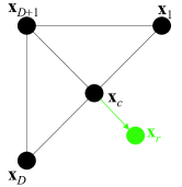
(a) Reflection

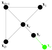
(b) Expansion

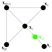
(c) Outside contraction

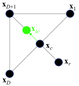
(d) Inside contraction

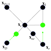
(e) Shrinkage

Figure 1: The geometric transformations in NM simplex search.

2.3. Quadratic interpolation  

$$x_{d}^{QI}=0.5\frac{\left[\left(x_{d}^{best})^{2}-(x_{d}^{b})^{2}\right)\right]f\left(\mathbf{x}^{a}\right)+\left[\left(x_{d}^{a})^{2}-(x_{d}^{best})^{2}\right)\right]f\left(\mathbf{x}^{b}\right)+\left[\left(x_{d}^{b})^{2}-(x_{d}^{a})^{2}\right)\right]f\left(\mathbf{x}^{best}\right)}{\left(x_{d}^{best}-x_{d}^{b}\right)f\left(\mathbf{x}^{a}\right)+\left(x_{d}^{a}-x_{d}^{best}\right)f\left(\mathbf{x}^{b}\right)+\left(x_{d}^{b}-x_{d}^{a}\right)f\left(\mathbf{x}^{best}\right)},\ d=1,2,\ldots,D$$ (16)

QI is an analytical local search method which utilizes a parabola to fit the shape of the objective function. This method is capable to strengthen the exploitation capacity. In QI, three known points are used as the QI search agents to generate a quadratic curve, the generated quadratic curve is used as the approximate shape of the objective function, and the extreme point of the quadratic function can be used to approximate the optima of the objective function [20]. Theoretically, when the the QI search agents are close enough to the global minimum, shape of the target function can be well approximated by the generated quadratic curve.

For a D-dimensional problem, three QI search agents $\mathbf{x}^{a}$, $\mathbf{x}^{b}$ and $\mathbf{x}^{best}$ are selected to generate a new solution $\mathbf{x}^{QI}$. Suppose that

$$\mathbf{x}^{a}=\left(x_{1}^{a},x_{2}^{a},\ldots,x_{D}^{a}\right),$$

$$\mathbf{x}^{b}=\left(x_{1}^{b},x_{2}^{b},\ldots,x_{D}^{b}\right),$$

$$\mathbf{x}^{best}=\left(x_{1}^{best},x_{2}^{best},\ldots,x_{D}^{best}\right)$$

are the three distinct search agents, then the new solution

$$\mathbf{x}^{QI}=\left(x_{1}^{QI},x_{2}^{QI},\ldots,x_{D}^{QI}\right)$$

can be calculated as Eq. (16), where $f\left(\mathbf{x}^{a}\right)$, $f\left(\mathbf{x}^{b}\right)$ and $f\left(\mathbf{x}^{best}\right)$ are the fitness values of the three search agents respectively. As a strong local search method, QI is capable to strengthen the exploitation capacity but could easily lead to a local minimum. Therefore, QI should only be invoked in later stage of the search.

3 Proposed method

3.1. NM-POSTA  

In POSTA, the historical information is not utilized sufficiently. As shown in Fig. 2(a) and Fig. 3(a) , the historical information is utilized by translation operator. However, only the latest two historical solutions are collected and only a linear search is applied to utilize the information. This inefficiency leads to the low convergence speed of POSTA on specific problems.

In the past decades, combining NM simplex search with metaheuristic methods has been a popular way to speed up the convergence. The general combination strategies between NM simplex search and metaheuristic methods can be summarized into two types: the staged pipelining type combination and the eagle strategy type combination [21]. In the first type, NM simplex search is applied to the superior individuals in the population [22]. In the second type, NM simplex search is applied in the exploitation stage as a local search method [23, 10]. But none of the existing combinations have seen NM simplex search as a way to utilize the information of historical solutions.

In this section, a POSTA enhanced with NM simplex search (NM-POSTA) is proposed. In NM-POSTA, a historical information mechanism based on NM simplex search is proposed to make use of the historical information. In the proposed mechanism, the historical information is collected based on a collection strategy, stored in the NM simplex, and then utilized by the NM geometric transformations. The detailed historical information mechanism in NM-POSTA is illustrated as follows.

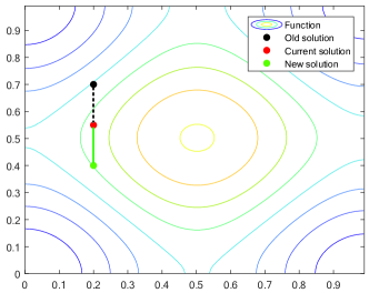
(a) Translation operator

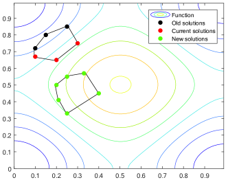
(b) The proposed mechanism

Figure 2: Comparison in utilizing history information.

A. The historical information set

In NM-POSTA, a historical information set called H is used to store the historical solutions generated by the state transformation operators. H has the capacity to store the coordinates of $D+1$ vertices in D-dimensional space. Therefore H can be seen as an NM simplex. For a D-dimensional problem, H is capable to store the information of $D+1$ historical solutions.

The historical information contained in H is more sufficient than that in the translation operator. As shown in Fig. 2 and Fig. 3, H contains information about a set of old solutions and a set of current solutions, but only an old solution and a current solution are considered in translation operator.

B. Utilization of the historical information

Algorithm 1 Utilize historical information based on NM geometric transformations.

1:Updated historical information set H

2:New historical information set H, $Best$

3:initial simplex $\leftarrow$ H

4:for each $i\in[1,D+1]$ do

5:     NM geometric transformations

6:end for

7:H $\leftarrow$ new  simplex

8:$Best$ $\leftarrow$ best solution in H

In NM-POSTA, the NM geometric transformations are applied for utilization. As shown in Fig. 1, the NM geometric transformations consists of a sequence of distinct geometric transformations, which are more comprehensive than the linear transformation in translation operator. As a result, NM-POSTA is able to utilize the historical information more comprehensively, as shown in Fig. 2 and Fig. 3.

The detailed steps of utilizing historical information in NM-POSTA is illustrated in Algorithm 1. When Algorithm 1 is invoked, H is input as the initial simplex. After that, the NM geometric transformations are applied to the initialized simplex. In the inner iterations, the NM geometric transformations are run for $D+1$ times.

Considering that each iteration of NM geometric transformations produces a new vertex approximately, running $D+1$ times approximately produces a new simplex with $D+1$ new vertices. Therefore a new simplex with $D+1$ new vertices is generated, and is then stored in H. As shown in Fig. 3(b), the new H contains $D+1$ new solutions and the top solution in H is denoted as $Best$. $Best$ is then sent to the state transformation operators as the input of current best solution.

C. Collection of historical information

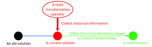
(a) Translation operator

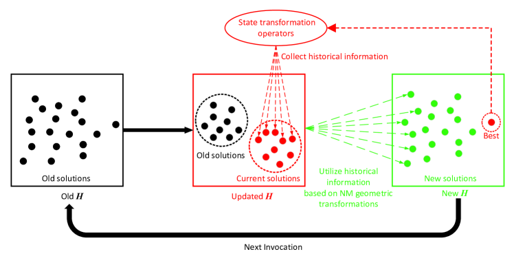
(b) The proposed mechanism

Figure 3: Comparison in collecting and utilizing historical information.

An appropriate collection strategy of history information is proposed to provide more promising input for utilization. Overall, the historical information is collected based on the collection strategy, stored in H and utilized by the NM geometric transformations. The utilization of historical information in NM-POSTA is illustrated in Algorithm 1. If an invocation of utilization is terminated, then the historical information needs to be re-collected before next utilization. Therefore, between the invocations of utilization, a collection strategy for historical information is considered.

In the collection strategy, two type of solutions are considered: old solutions and current solutions. As shown in 3(b), old solutions are the solutions generated in the last invocation of utilization. After the termination of the last utilization, the state transformation operators start to generate solutions from $Best$. Between the invocations of utilization, those solutions generated by POSTA are considered as current solutions.

This collection strategy is seen as an expanded version of that in the translation operator. As shown in Fig. 2(a) and Fig. 3(a), translation operator uses an old solution and a current solution as the historical information. In NM-POSTA, a set of old solutions and a set of current solutions are used as the historical information, as shown in Fig. 2(b) and Fig. 3(b).

Algorithm 2 Collect historical information

1:Old historical information set H, current solution $\mathbf{x}_{current}$

2:Updated historical information set H

3:replace the worst solution in H with $\mathbf{x}_{current}$

4:return updated H

The collection strategy is implemented by updating H. As shown in Algorithm 2, a current solution $\mathbf{x}_{current}$ is used to update H in an invocation. In the implementation, Algorithm 2 is invoked iteratively to update H with multiple current solutions. As shown in Fig. 3(b), H is updated by multiple current solutions before been utilized. To control the ratio between old solutions and current solutions in H, a parameter named update rate (UR) is proposed:

$$UR=\frac{n_{cs}}{n_{os}+n_{cs}}$$

where $n_{os}$ and $n_{cs}$ are namely the number of old solutions and the number of current solutions in H. As shown in Fig. 5, $UR$ is calculated after each update, and only when $UR$ exceeds certain threshold value will the utilization be invoked.

3.2. Properties of NM-POSTA  

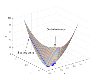
(a) Solution path of POSTA

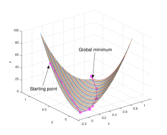
(b) Solution path of NM-POSTA

Figure 4: Solution paths of POSTA and NM-POSTA on Rosenbrock function.

In this section, some properties of NM-POSTA are briefly illustrated by a comparison between NM-POSTA and POSTA. To illustrate the effect of utilizing historical information, two classical test functions are used, namely Rosenbrock (F3) and Rastrigin (F7) from Table 2. NM-POSTA and POSTA are tested against the two functions in 2-D space and each method is only terminated when certain criterion is satisfied. After termination, the corresponding number of function evaluations (FEs) is recorded. For both POSTA and NM-POSTA, $SE$ is set to 50 and $T_{p}$ is set to 10. In NM-POSTA, threshold value for $UR$ is set to 0.5 and parameters in NM simplex search are set as: $\{\eta,\ \lambda,\ \mu,\ \nu\}=\{1,\ 2,\ 0.5,\ 0.5\}$, which are the same as that in the standard implementation of NM simplex search [7].

A. Faster convergence speed

Table 1: Table 1: Statistical results for POSTA and NM-POSTA with D = 2.

function	POSTA			NM-POSTA
	Ave FEs	Success rate		Ave FEs	Success rate
F3	1.08E+04	30/30		4.54E+03	30/30
F7	1.51E+03	30/30		1.47E+03	30/30

To demonstrate the faster convergence speed of NM-POSTA, a 2-D Rosenbrock test function is used. This unimodal function has a global minimum (1,1) that lies in a narrow, parabolic valley. The valley is easy to reach but further convergence is very difficult [24]. In the test for Rosenbrock function, the methods are terminated if the current solution $\mathbf{x}_{current}$ satisfies:

$$\left|{f}(\mathbf{x}_{current})-{f}({Best}^{*})\right|\leq\epsilon$$

where ${Best}^{*}$ indicates the global minimum. If the specified accuracy $\epsilon$ is met, the test is considered a ‘success’. In this section, $\epsilon$ is set at 1e-8.

The statistical results given in Table 1 reveal that NM-POSTA is able to reach the same accuracy with much less FEs. In Fig. 4, the solution paths of POSTA and NM-POSTA on the Rosenbrock function are portrayed, where both methods start from the starting point (0, 0.75) and only the first 10 solutions are plotted in the figures for the convenience of observation. It is obvious that the solution path of NM-POSTA is much more efficient. By comparing the two paths, it can be seen that the both methods quickly reach the valley. After that, POSTA searches aimlessly in the valley and moves slowly while NM-POSTA finds the promising direction and moves towards the optimum efficiently. This brief experiment demonstrates that the utilization of historical information can lead to a more promising search direction, therefore NM-POSTA has a faster convergence speed than POSTA.

B. Consistent global stability

To demonstrate the stability on avoiding local minimums, a 2-D Rastrigin test function is used. This function is a multimodal function with many local minimums.

In the test for Rastrigin function, the methods are only terminated when the global optimum is found. If the global minimum is found, the test is considered a ‘success’. The statistical results given in Table 1 show that NM-POSTA gets the same success rate with slightly less FEs. It is obvious from the results that the NM-POSTA remains stable in avoiding local minimums.

3.3. The enhanced POSTA (NMQI-POSTA)  

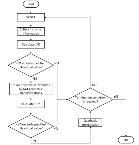
Figure 5: Flow chart of the enhanced POSTA.

POSTA, NM simplex search and QI are methods with distinct characteristics. As a novel metaheuristic method, POSTA has strong global exploration capacity but lacks convergence speed and exploitation capacity. As a classical direct search method, NM simplex search has a fast convergence speed but is not stable in global search. QI is able to approximate the global minimum by an analytical solution but is only effective when the search agents are very close to the global minimum.

To combine the merits of the three methods, NM simplex search and QI are applied to utilize the historical information of POSTA. Therefore, an enhanced POSTA based on NM simplex search and QI (NMQI-POSTA) is proposed. As shown in Fig. 5, the proposed method uses an eagle strategy [25] to maximize the efficiency and stability. In the exploration stage, NM simplex search utilizes the historical information of POSTA to generate promising solutions. As a result, the convergence speed is continuously accelerated. In the exploitation stage, QI utilizes the historical information to improve the local search capacity. As a result, the solution accuracy is increased.

To invoke QI in later stage of the search, the average accuracy of the solutions in the historical information set H is calculated in each iteration as:

$$\small AAS=\left|\frac{f\left(\textbf{x}_{1}\right)+f\left(\textbf{x}_{2}\right)+\ldots+f\left(\textbf{x}_{D+1}\right)}{D+1}-{f}({Best}^{*})\right|$$

where ${Best}^{*}$ indicates the global best solution.

If $AAS$ meets the certain threshold value, the solutions are considered to be in the neighborhood of the global optimum. Then QI will be invoked to increase the solution accuracy. In the implementation of QI, two QI search agents $\textbf{x}^{a}$ and $\textbf{x}^{b}$ are randomly chosen from the historical information set H and the third search agent $\textbf{x}^{best}$ is the current best solution.

For comparison, a POSTA enhanced with QI (QI-POSTA) is also implemented. The strategy of QI-POSTA is basically the same as NMQI-POSTA. The only difference is that the NM simplex search is disabled in QI-POSTA.

4 Experimental results and discussions

In this section, the proposed method is tested against a set of benchmark functions. To guarantee fairness and avoid arbitrariness, each test in the following experiments is performed 30 times independently. All methods are implemented in MATLAB R2017b environment with an AMD R7-4800H, 2.90 GHz processor on a 64-bit Windows 10 operating system.

Table 2: Table 2: Benchmark function set.

Funtion name	Equation	Range	${f}_{\min}$	Modality
Elliptic	$\mathrm{F}1=\sum_{i=2}^{D}\left(10^{6}\right)^{(i-1)/(D-1)}\cdot x_{i}^{2}$	$[-100,100]$	0	Unimodal
Penalized 1	$\begin{array}[]{c}\mathrm{F}2=\frac{\pi}{D}\left\{\sum_{t=1}^{D-1}\left(y_{i}-1\right)^{2}\left[1+\sin\left(\pi y_{i+1}\right)\right]+\left(y_{D}-1\right)^{2}+\right.\\ \left.\left(10\sin^{2}\left(\pi y_{1}\right)\right)\right\}+\sum_{i=1}^{D}u\left(x_{i},10,100,4\right)\\ y_{i}=1+\frac{x_{1}+1}{4}\\ u\left(x_{i},a,k,m\right)=\left\{\begin{array}[]{ll}k\left(x_{i}-a\right)^{m},&x_{i}>a\\ 0,&-a\leq x_{i}\leq a\\ k\left(-x_{i}-a\right)^{m},&x_{i}<-a\end{array}\right.\end{array}$	$[-50,50]$	0	Multimodal
Rosenbrock	$\mathrm{F}3=\sum_{i=1}^{D-1}\left[100\left(x_{i+1}-x_{i}^{2}\right)^{2}+\left(x_{i}-1\right)^{2}\right]$	$[-30,30]$	0	Unimodal
Schwefel 1.2	$\mathrm{F}4=\sum_{i=1}^{D}\left(\sum_{j=1}^{1}x_{j}\right)^{2}$	[-100,100]	0	Unimodal
Schwefel 2.4	$\mathrm{F}5=\sum_{i=1}^{D}\left[\left(x_{i}-1\right)^{2}+\left(x_{1}-x_{i}^{2}\right)^{2}\right]$	[0,10]	0	Multimodal
Sphere	$\mathrm{F}6=\sum_{i=1}^{D}x_{i}^{2}$	[-100,100]	0	Unimodal
Rastrigin	$\mathrm{F}7=\sum_{i=1}^{D}\left[x_{i}^{2}-10\cos\left(2\pi x_{i}\right)+10\right]$	[-5.12,5.12]	0	Multimodal
Griewank	$\mathrm{F}8=\sum_{i=1}^{D}\frac{x_{i}^{2}}{4000}-\prod_{i=1}^{D}\cos\left(x_{i}/\sqrt{i}\right)+1$	[-60,60]	0	Multimodal
Sum squares	$\mathrm{F}9=\sum_{i=2}^{D}ix_{i}^{2}$	[-10,10]	0	Unimodal
Levy and Montalvo 1	$\begin{array}[]{c}\mathrm{F}10=\frac{\pi}{D}\left(10\sin^{2}\left(\pi y_{1}\right)+\sum_{i=1}^{D-1}\left(y_{i}-1\right)^{2}[1+\right.\\ \left.\left.10\sin^{2}\left(\pi y_{i+1}\right)\right]+\left(y_{D}-1\right)^{2}\right),\quad y_{i}=1+\frac{1}{4}\left(x_{i}+1\right)\end{array}$	[-10,10]	0	Multimodal
Zakharov	$\mathrm{F}11=\sum_{i=1}^{D}x_{i}^{2}+\left(\sum_{i=1}^{D}0.5ix_{i}\right)^{2}+\left(\sum_{i=1}^{D}0.5ix_{i}\right)^{4}$	[-5,10]	0	Unimodal
Schwefel 2.2.2	$\mathrm{F}12=\sum_{i=1}^{D}\left|x_{i}\right|+\prod_{i=1}^{D}\left|x_{i}\right|$	[-10,10]	0	Unimodal
Cigar	$\mathrm{F}13=x_{1}^{2}+10^{6}\sum_{i-2}^{D}x_{i}^{6}$	[-100,100]	0	Unimodal
Csendes	$\mathrm{F}14=\sum_{i=1}^{D}x_{i}^{6}\left(2+\sin\frac{1}{x_{i}}\right)$	[-1,1]	0	Multimodal

In Section 4.2, the POSTA families (POSTA, NM-POSTA, QI-POSTA and NMQI-POSTA) are comprehensively tested against the benchmark functions. In Section 4.3, the enhanced POSTA is compared with several metaheuristic methods on the benchmark functions.

4.1. Benchmark functions and parameter settings  

The details of the benchmark functions are shown in Table 2. Notably, ${f}_{\min}$ and $Range$ indicate the global optimal value of the objective function and the boundary of the search space. Generally, in Table 2, there are two types of benchmark functions, called unimodal and multimodal. A function with a single minimum in the specified range is called unimodal. Unlike unimodal, multimodal functions have many local minimums that the method may be trapped in.

For all members in the POSTA family, $SE$ is set to 50 and $T_{p}$ is set to 10. In NM-POSTA, threshold value for $UR$ is set to 0.5. In QI-POSTA and NMQI-POSTA, threshold value for $AAS$ is set to 1e-6. To guarantee fairness for the comparison in Section 4.3, the population sizes in the other metaheuristic methods are all set to 50, which are the same as the value of parameter $SE$ in the enhanced POSTA.

4.2. Comparison among the POSTA families  

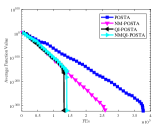
(a) F1

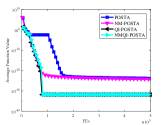
(b) F2

(c) F3

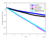
(d) F4

(e) F5

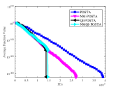
(f) F6

(g) F7

(h) F8

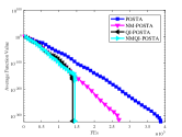
(i) F9

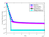
(j) F10

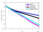
(k) F11

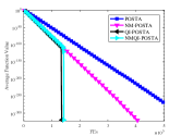
(l) F12

(m) F13

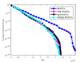
(n) F14

Figure 6: Average convergence curves of the POSTA families on benchmark functions with D = 30.

To comprehensively verify the effect of NM simplex search and QI in the proposed method, the POSTA families (POSTA, NM-POSTA, QI-POSTA and NMQI-POSTA) are tested against the benchmark functions listed in Table 2. For each benchmark function, the number of decision variables $D$ is set to 20, 30, and 50. For each independent test, the maximum number of function evaluations is set at $5e3*D*log(D)$. In an independent test, a method is terminated if any of the following criteria is satisfied:

• The global minimum of the objective function is found.

• The maximum number of function evaluations is attained.

After termination, the best solution attained and the number of function evaluations (FEs) used in this single test are recorded. The statistical results are shown in Tables 3-5 and the average convergence curves are given in Fig. 6.

The experimental results demonstrate that NM simplex search speeds up the convergence while maintaining stable, as shown in Tables 3-5 and Fig. 6. For functions like F3 and F4, POSTA suffers from a relatively low convergence speed but NM-POSTA significantly improves the speed by utilizing historical information. For function F1, F6, F9, F11, F12, F13 and F14, POSTA already gives an acceptable performance but NM-POSTA further accelerates the search process and reduces the average FEs. For multimodal functions like F2, F5, F7, F8 and F10, NM-POSTA remains stable in avoiding local minimums.

The experimental results also demonstrate that QI improves the solution accuracy and maintains stable in global exploration. As shown in Fig. 6, POSTA becomes very slow in the exploitation stage on F2, F5 and F10, but QI-POSTA produces solutions with much better accuracy. At the same time, for F1, F6, F9, F11, F12, F13 and F14, QI further reduces the average FEs. Also, the statistical results in Tables 3-5 reveal that the stability in multimodal functions is remained because QI is only invoked when the solutions are close to the global minimum.

Note that both NM simplex search and QI are capable to reduce the average FEs on these functions, but the approaches are different: NM simplex search utilizes historical information during the whole search, so that the whole convergence is accelerated, and therefore the average FEs is reduced. On the other hand, QI utilizes historical information in later stage search, so that an analytical solution $\mathbf{x}^{QI}$ with high accuracy is generated. $\mathbf{x}^{QI}$ usually has the accuracy that is high enough to meet the termination conditions. Therefore the later stage of the search is ‘skipped’ and the average FEs is reduced. As shown in Fig. 6, the whole search is accelerated in NM-POSTA, and the later stage is ‘skipped’ in QI-POSTA.

Table 3: Table 3: Statistical results for POSTA families with D = 20.

function	POSTA		NM-POSTA		QI-POSTA		NMQI-POSTA
	Mean(Std)	Ave FEs	Mean(Std)	Ave FEs	Mean(Std)	Ave FEs	Mean(Std)	Ave FEs
F1	0.00E+00(0.00E+00)	2.79E+05	0.00E+00(0.00E+00)	1.93E+05	0.00E+00(0.00E+00)	9.90E+04	0.00E+00(0.00E+00)	1.05E+05
F2	1.71E-24(8.14E-25)	3.01E+05	9.16E-25(5.61E-25)	3.01E+05	2.36E-32(8.35E-48)	3.01E+05	2.36E-32(8.35E-48)	3.01E+05
F3	8.22E+00(2.29E-01)	3.03E+05	5.32E-19(8.97E-19)	3.01E+05	5.86E+00(1.79E+00)	3.01E+05	0.00E+00(0.00E+00)	2.13E+05
F4	3.67E-26(1.59E-25)	3.01E+05	3.41E-58(8.38E-58)	3.01E+05	1.65E-34(6.19E-34)	3.01E+05	3.28E-59(1.09E-58)	3.01E+05
F5	1.19E-21(6.66E-22)	3.01E+05	4.49E-22(3.85E-22)	3.01E+05	0.00E+00(0.00E+00)	5.00E+04	0.00E+00(0.00E+00)	4.98E+04
F6	0.00E+00(0.00E+00)	2.89E+05	0.00E+00(0.00E+00)	1.98E+05	0.00E+00(0.00E+00)	1.01E+05	0.00E+00(0.00E+00)	1.05E+05
F7	0.00E+00(0.00E+00)	2.77E+04	0.00E+00(0.00E+00)	1.96E+04	0.00E+00(0.00E+00)	2.13E+04	0.00E+00(0.00E+00)	1.86E+04
F8	9.40E-03(3.01E-02)	9.42E+04	1.10E-02(3.03E-02)	7.69E+04	6.23E-03(1.98E-02)	7.83E+04	9.91E-03(2.71E-02)	8.64E+04
F9	2.50e-323(0.00E+00)	2.90E+05	0.00E+00(0.00E+00)	1.96E+05	0.00E+00(0.00E+00)	1.00E+05	0.00E+00(0.00E+00)	1.05E+05
F10	1.75E-24(7.30E-25)	3.01E+05	8.59E-25(4.08E-25)	3.01E+05	2.36E-32(8.35E-48)	3.01E+05	2.36E-32(8.35E-48)	3.01E+05
F11	6.69E-44(3.66E-43)	3.01E+05	1.71E-85(9.31E-85)	3.01E+05	1.56E-59(8.52E-59)	3.01E+05	4.13E-86(1.63E-85)	3.01E+05
F12	4.12E-203(0.00E+00)	3.01E+05	2.10E-296(0.00E+00)	3.01E+05	0.00E+00(0.00E+00)	1.09E+05	0.00E+00(0.00E+00)	1.13E+05
F13	0.00E+00(0.00E+00)	1.74E+05	0.00E+00(0.00E+00)	1.18E+05	0.00E+00(0.00E+00)	1.16E+05	0.00E+00(0.00E+00)	1.07E+05
F14	0.00E+00(0.00E+00)	1.73E+05	0.00E+00(0.00E+00)	1.30E+05	0.00E+00(0.00E+00)	1.32E+05	0.00E+00(0.00E+00)	1.33E+05

Table 4: Table 4: Statistical results for POSTA families with D = 30.

function	POSTA		NM-POSTA		QI-POSTA		NMQI-POSTA
	Mean(Std)	Ave FEs	Mean(Std)	Ave FEs	Mean(Std)	Ave FEs	Mean(Std)	Ave FEs
F1	0.00E+00(0.00E+00)	3.77E+05	0.00E+00(0.00E+00)	2.63E+05	0.00E+00(0.00E+00)	1.32E+05	0.00E+00(0.00E+00)	1.40E+05
F2	1.49E-24(5.46E-25)	5.12E+05	7.93E-25(4.16E-25)	5.12E+05	1.57E-32(5.57E-48)	5.12E+05	1.57E-32(5.57E-48)	5.12E+05
F3	2.02E+01(1.74E+01)	5.13E+05	8.94E-18(2.46E-17)	5.12E+05	2.01E+01(1.91E+01)	5.12E+05	0.00E+00(0.00E+00)	3.18E+05
F4	2.01E-20(6.89E-20)	5.12E+05	1.25E-74(3.78E-74)	5.12E+05	1.47E-25(6.19E-25)	5.12E+05	6.23E-74(3.28E-73)	5.12E+05
F5	1.76E-21(6.05E-22)	5.12E+05	4.56E-22(3.37E-22)	5.12E+05	0.00E+00(0.00E+00)	8.04E+04	0.00E+00(0.00E+00)	6.94E+04
F6	0.00E+00(0.00E+00)	3.90E+05	0.00E+00(0.00E+00)	2.72E+05	0.00E+00(0.00E+00)	1.38E+05	0.00E+00(0.00E+00)	1.46E+05
F7	0.00E+00(0.00E+00)	5.89E+04	0.00E+00(0.00E+00)	3.25E+04	0.00E+00(0.00E+00)	3.24E+04	0.00E+00(0.00E+00)	3.35E+04
F8	0.00E+00(0.00E+00)	4.26E+04	0.00E+00(0.00E+00)	2.94E+04	0.00E+00(0.00E+00)	4.85E+04	0.00E+00 (0.00E+00)	2.91E+04
F9	0.00E+00(0.00E+00)	3.88E+05	0.00E+00(0.00E+00)	2.68E+05	0.00E+00(0.00E+00)	1.39E+05	0.00E+00(0.00E+00)	1.45E+05
F10	1.33E-24(4.26E-25)	5.12E+05	6.01E-25(3.10E-25)	5.12E+05	1.57E-32(5.57E-48)	5.12E+05	1.57E-32(5.57E-48)	5.12E+05
F11	1.40E-41(4.06E-41)	5.12E+05	1.20E-86(3.70E-86)	5.12E+05	7.10E-56(2.76E-55)	5.12E+05	4.97E-86(1.77E-85)	5.12E+05
F12	6.97E-280(0.00E+00)	5.14E+05	0.00E+00(0.00E+00)	4.07E+05	0.00E+00(0.00E+00)	1.36E+05	0.00E+00(0.00E+00)	1.43E+05
F13	8.17E-218(0.00E+00)	4.43E+05	0.00E+00(0.00E+00)	3.59E+05	0.00E+00(0.00E+00)	3.05E+05	0.00E+00(0.00E+00)	2.75E+05
F14	2.97E-272(0.00E+00)	4.34E+05	0.00E+00(0.00E+00)	3.25E+05	1.48E-299(0.00E+00)	3.38E+05	0.00E+00(0.00E+00)	3.30E+05

Table 5: Table 5: Statistical results for POSTA families with D = 50.

function	POSTA		NM-POSTA		QI-POSTA		NMQI-POSTA
	Mean(Std)	Ave FEs	Mean(Std)	Ave FEs	Mean(Std)	Ave FEs	Mean(Std)	Ave FEs
F1	0.00E+00(0.00E+00)	5.84E+05	0.00E+00(0.00E+00)	4.23E+05	0.00E+00(0.00E+00)	2.17E+05	0.00E+00(0.00E+00)	2.24E+05
F2	9.85E-25(2.38E-25)	9.80E+05	4.59E-25(1.85E-25)	9.80E+05	9.42E-33(2.78E-48)	9.80E+05	9.42E-33(2.78E-48)	9.80E+05
F3	4.44E+01(2.31E+01)	9.80E+05	1.42E-16(1.74E-16)	9.80E+05	3.40E+01(1.94E+01)	9.80E+05	0.00E+00(0.00E+00)	6.61E+05
F4	1.18E-12(2.07E-12)	9.80E+05	1.38E-87(7.50E-87)	9.80E+05	7.79E-17(1.43E-16)	9.80E+05	7.21E-86(3.94E-85)	9.80E+05
F5	2.89E-21(9.30E-22)	9.80E+05	2.10E-21(1.29E-21)	9.80E+05	0.00E+00(0.00E+00)	1.41E+05	0.00E+00(0.00E+00)	9.49E+04
F6	0.00E+00(0.00E+00)	6.24E+05	0.00E+00(0.00E+00)	4.61E+05	0.00E+00(0.00E+00)	2.42E+05	0.00E+00(0.00E+00)	2.63E+05
F7	3.60E-14(7.08E-14)	4.08E+05	4.17E-14(8.70E-14)	3.52E+05	3.79E-14(7.51E-14)	3.25E+05	5.12E-14(8.22E-14)	4.61E+05
F8	0.00E+00(0.00E+00)	7.33E+04	0.00E+00(0.00E+00)	5.51E+04	0.00E+00(0.00E+00)	6.54E+04	0.00E+00(0.00E+00)	5.93E+04
F9	0.00E+00(0.00E+00)	6.38E+05	0.00E+00(0.00E+00)	4.43E+05	0.00E+00(0.00E+00)	2.32E+05	0.00E+00(0.00E+00)	2.47E+05
F10	9.15E-25(2.12E-25)	9.80E+05	5.12E-25(2.03E-25)	9.80E+05	9.42E-33(2.78E-48)	9.80E+05	9.42E-33(2.78E-48)	9.80E+05
F11	1.54E-38(3.96E-38)	9.80E+05	2.53E-105(8.38E-105)	9.80E+05	6.76E-50(3.35E-49)	9.80E+05	1.86E-106(4.36E-106)	9.80E+05
F12	0.00E+00(0.00E+00)	7.47E+05	0.00E+00(0.00E+00)	5.30E+05	0.00E+00(0.00E+00)	1.74E+05	0.00E+00(0.00E+00)	1.85E+05
F13	7.33E-276(0.00E+00)	9.79E+05	0.00E+00(0.00E+00)	7.91E+05	0.00E+00(0.00E+00)	6.07E+05	0.00E+00(0.00E+00)	6.03E+05
F14	6.39E-191(0.00E+00)	9.80E+05	2.10E-267(0.00E+00)	9.80E+05	7.44E-259(0.00E+00)	9.80E+05	2.26E-266(0.00E+00)	9.80E+05

As mentioned above, NM simplex search is applied during the whole search. But QI is only invoked in later stage. As shown in Fig. 6(c), QI-POSTA shows no advantage over POSTA on F3 because POSTA has a low convergence speed on F3 and is not able to reach the neighborhood of the global minimum. But in NMQI-POSTA, QI is quite effective because NM-POSTA is able to reach the neighborhood of the global minimum.

From the above discussion, it can be observed that when POSTA is enhanced with both NM simplex search and QI, the merits of the three distinct methods are combined. The convergence curves and the statistical results show that NMQI-POSTA enjoys the merits of the three: global exploration capacity of POSTA, fast convergence speed of NM simplex search and deep exploitation capacity of QI.

4.3. Comparison with other meteheuristic methods  

To examine the effectiveness of the enhanced POSTA, several population-based metaheuristic methods are used in this section, including ABC [26, 27], SaDE [28, 29], GWO [30, 31] and CLPSO [32, 33]. For each benchmark function, the number of decision variables $D$ is set to 20, 30, and 50. For each independent test, the maximum function evaluations is set at $5e3*D*log(D)$.

Table 6: Table 6: Statistical results for different metaheuristic methods with D = 20.

function	ABC	GWO	SaDE	CLPSO	NMQI-POSTA
	Mean(Std)	Mean(Std)	Mean(Std)	Mean(Std)	Mean(Std)
F1	3.42E+03(2.99E+03)-	0.00E+00(0.00E+00)$\approx$	3.93E-201(0.00E+00)-	1.20E-33(1.73E-33)-	0.00E+00(0.00E+00)
F2	2.64E-02(3.75E-02)-	1.70E-02(7.90E-03)-	2.36E-32(8.35E-48)$\approx$	2.36E-32(8.35E-48$\approx$	2.36E-32(8.35E-48)
F3	4.65E+02(2.64E+02)-	1.63E+01(6.38E-01)-	9.81E+00(2.84E+00)-	2.19E+00(2.30E+00)-	0.00E+00(0.00E+00)
F4	1.02E+04(2.06E+03)-	1.53E-301(0.00E+00)+	3.22E-20(7.57E-20)-	7.86E+00(2.53E+00)-	3.28E-59(1.09E-58)
F5	1.12E+01(1.01E+01)-	3.84E+00(1.21E+00)-	1.58E-30(7.61E-31)-	3.25E-05(7.76E-06)-	0.00E+00(0.00E+00)
F6	4.26E-01(3.24E-01)-	0.00E+00(0.00E+00)$\approx$	1.73E-197(0.00E+00)-	2.90E-37(2.62E-37)-	0.00E+00(0.00E+00)
F7	1.09E+01(2.10E+00)-	0.00E+00(0.00E+00)$\approx$	0.00E+00(0.00E+00)$\approx$	0.00E+00(0.00E+00)$\approx$	0.00E+00(0.00E+00)
F8	5.92E-01(1.51E-01)-	0.00E+00(0.00E+00)+	5.75E-04(2.21E-03)$\approx$	2.59E-17(9.07E-17)$\approx$	9.91E-03(2.71E-02)
F9	4.45E-02(2.51E-02)-	0.00E+00(0.00E+00)$\approx$	2.38E-199(0.00E+00)-	2.16E-38(1.64E-38)-	0.00E+00(0.00E+00)
F10	1.00E-04(1.22E-04)-	1.82E-02(1.03E-02)-	2.36E-32(8.35E-48)$\approx$	2.36E-32(8.35E-48)$\approx$	2.36E-32(8.35E-48)
F11	1.70E+02(2.49E+01)-	0.00E+00(0.00E+00)+	1.26E-33(3.95E-33)-	5.69E-04(1.78E-04)-	4.13E-86(1.63E-85)
F12	1.54E-01(3.88E-02)-	0.00E+00(0.00E+00)$\approx$	2.18E-107(2.80E-107)-	1.99E-22(1.04E-22)-	0.00E+00(0.00E+00)
F13	3.02E+04(9.22E+04)-	0.00E+00(0.00E+00)$\approx$	7.55e-311(0.00E+00)-	2.08E-66(3.88E-66)-	0.00E+00(0.00E+00)
F14	7.69E-14(2.55E-13)-	0.00E+00(0.00E+00)$\approx$	0.00E+00(0.00E+00)$\approx$	1.34E-78(2.15E-78)-	0.00E+00(0.00E+00)
+/$\approx$/-	0/0/14	3/7/4	0/5/9	0/4/10	-/-/-

The computational results are listed in Tables 6-8 and the average convergence curves of all test functions with $D=30$ are given in Fig. 7. In Tables 6-8, the symbols -, +, $\approx$ indicate the results of Wilcoxon rank sum test [34, 35] with a significance level of 0.05. Correspondingly, the symbol - indicates that the performance is significantly worse than the proposed method, the symbol + indicates that the performance is significantly better than the proposed method, and the symbol $\approx$ indicates that the performance difference is not statistically significant compared to the proposed method.

As shown in the experiment results, the enhanced POSTA outperforms CLPSO, SaDE and ABC in most of the cases. Despite GWO gives better performance on functions like F4 and F11, it failed to remain stable in finding acceptable solutions on F2, F3, F5 and F10. On the contrary, the enhanced POSTA shows incomparably convergence speed and solution accuracy on F3 and F5, and shows more robustness on multimodal functions like F2 and F10. Therefore, the proposed method is more effective and robust than these competitive metaheuristic methods.

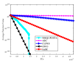
(a) F1

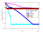
(b) F2

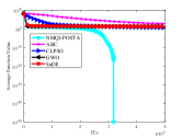
(c) F3

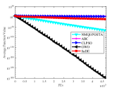
(d) F4

(e) F5

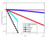
(f) F6

(g) F7

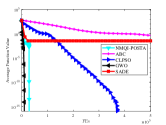
(h) F8

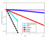
(i) F9

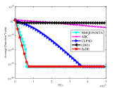
(j) F10

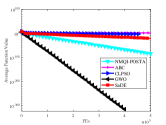
(k) F11

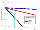
(l) F12

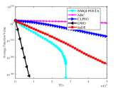
(m) F13

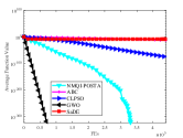
(n) F14

Figure 7: Average convergence curves of different metaheuristic methods on benchmark functions with D = 30.

Table 7: Table 7: Statistical results for different metaheuristic methods with D = 30.

function	ABC	GWO	SaDE	CLPSO	NMQI-POSTA
	Mean(Std)	Mean(Std)	Mean(Std)	Mean(Std)	Mean(Std)
F1	2.53E+03(1.88E+03)-	0.00E+00(0.00E+00)$\approx$	5.72E-231(0.00E+00)-	3.95E-39(3.51E-39)-	0.00E+00(0.00E+00)
F2	1.07E-02(1.13E-02)-	4.27E-02(1.38E-02)-	1.38E-02(7.57E-02)-	1.57E-32(5.57E-48)$\approx$	1.57E-32(5.57E-48)
F3	6.31E+02(3.37E+02)-	2.63E+01(6.65E-01)-	1.87E+01(1.55E+01)-	5.87E+00(1.39E+01)-	0.00E+00(0.00E+00)
F4	2.31E+04(2.93E+03)-	0.00E+00(0.00E+00)+	2.35E-13(1.03E-12)-	1.52E+02(4.31E+01)-	6.23E-74(3.28E-73)
F5	3.05E+01(1.45E+01)-	8.80E+00(8.62E-01)-	5.27E-30(1.83E-30)-	2.95E-05(6.95E-06)-	0.00E+00(0.00E+00)
F6	3.00E-01(2.01E-01)-	0.00E+00(0.00E+00)$\approx$	1.19E-224(0.00E+00)-	2.61E-42(1.72E-42)-	0.00E+00(0.00E+00)
F7	1.60E+01(2.54E+00)-	0.00E+00(0.00E+00)$\approx$	0.00E+00(0.00E+00)$\approx$	0.00E+00(0.00E+00)$\approx$	0.00E+00(0.00E+00)
F8	4.27E-01(1.21E-01)-	0.00E+00(0.00E+00)$\approx$	3.86E-03(8.49E-03)-	0.00E+00(0.00E+00)$\approx$	0.00E+00(0.00E+00)
F9	4.02E-02(2.32E-02)-	0.00E+00(0.00E+00)$\approx$	5.24E-226(0.00E+00)-	2.98E-43(2.53E-43)-	0.00E+00(0.00E+00)
F10	2.55E-05(2.79E-05)-	4.66E-02(1.63E-02)-	1.57E-32(5.57E-48)$\approx$	1.57E-32(5.57E-48)$\approx$	1.57E-32(5.57E-48)
F11	3.08E+02(3.11E+01)-	0.00E+00(0.00E+00)+	5.90E-21(2.09E-20)-	8.38E-03(3.13E-03)-	4.97E-86(1.77E-85)
F12	1.46E-01(3.54E-02)-	0.00E+00(0.00E+00)$\approx$	9.29E-136(1.74E-135)-	2.01E-25(8.32E-26)-	0.00E+00(0.00E+00)
F13	1.28E+04(4.48E+04)-	0.00E+00(0.00E+00)$\approx$	2.38E-245(0.00E+00)-	1.71E-77(6.14E-77)-	0.00E+00(0.00E+00)
F14	1.07E-14(2.08E-14)-	0.00E+00(0.00E+00)$\approx$	8.05E-09(2.89E-08)-	2.88E-86(3.84E-86)-	0.00E+00(0.00E+00)
+/$\approx$/-	0/0/14	2/8/4	0/2/12	0/4/10	-/-/-

Table 8: Table 8: Statistical results for different metaheuristic methods with D = 50.

function	ABC	GWO	SaDE	CLPSO	NMQI-POSTA
	Mean(Std)	Mean(Std)	Mean(Std)	Mean(Std)	Mean(Std)
F1	1.31E+03(8.41E+02)-	0.00E+00(0.00E+00)$\approx$	3.37E-237(0.00E+00)-	1.33E-46(6.70E-47)-	0.00E+00(0.00E+00)
F2	2.82E-03(1.86E-03)-	1.04E-01(2.34E-02)-	1.45E-02(3.13E-02)-	9.42E-33(2.78E-48)$\approx$	9.42E-33(2.78E-48)
F3	6.13E+02(1.92E+02)-	4.63E+01(7.82E-01)-	4.42E+01(2.78E+01)-	1.32E+01(1.84E+01)-	0.00E+00(0.00E+00)
F4	5.49E+04(5.14E+03)-	0.00E+00(0.00E+00)+	5.24E-08(8.90E-08)-	2.55E+03(4.70E+02)-	7.21E-86(3.94E-85)
F5	6.13E+01(2.15E+01)-	2.07E+01(1.71E+00)-	2.92E-29(1.32E-29)-	1.56E-05(2.08E-06)-	0.00E+00(0.00E+00)
F6	1.25E-01(6.41E-02)-	0.00E+00(0.00E+00)$\approx$	6.84E-235(0.00E+00)-	1.10E-49(5.63E-50)-	0.00E+00(0.00E+00)
F7	2.29E+01(2.47E+00)-	0.00E+00(0.00E+00)+	3.65E-01(6.12E-01)$\approx$	0.00E+0(0.00E+00)+	5.12E-14(8.22E-14)
F8	2.27E-01(1.01E-01-	0.00E+00(0.00E+00)$\approx$	9.30E-03(1.95E-02)-	0.00E+00(0.00E+00)$\approx$	0.00E+00(0.00E+00)
F9	2.68E-02(1.51E-02)-	0.00E+00(0.00E+00)$\approx$	2.27E-233(0.00E+00)-	2.52E-50(1.56E-50)-	0.00E+00(0.00E+00)
F10	8.33E-06(9.02E-06)-	9.69E-02(2.13E-02)-	9.42E-33(2.78E-48)$\approx$	9.42E-33(2.78E-48)$\approx$	9.42E-33(2.78E-48)
F11	6.29E+02(5.20E+01)-	0.00E+00(0.00E+00)+	3.14E-09(1.69E-08)-	1.99E-01(6.82E-02)-	1.86E-106(4.36E-106)
F12	1.11E-01(2.53E-02)-	0.00E+00(0.00E+00)$\approx$	4.89E-158(1.34E-157)-	8.50E-30(3.23E-30)-	0.00E+00(0.00E+00)
F13	6.76E+02(1.65E+03)-	0.00E+00(0.00E+00)$\approx$	1.55E-200(0.00E+00)-	7.03E-94(8.26E-94)-	0.00E+00(0.00E+00)
F14	2.08E-15(2.98E-15)-	0.00E+00(0.00E+00)+	6.66E-08(1.22E-07)$\approx$	1.34E-96(1.84E-96)-	2.26E-266(0.00E+00)
+/$\approx$/-	0/0/14	4/6/4	0/3/11	0/3/11	-/-/-

5 Conclusion

In this paper, an enhanced POSTA based on Nelder-Mead simplex search and QI is proposed. In the enhanced POSTA, both NM simplex search and QI are applied to utilize the historical information. Specifically, NM simplex search is applied in the whole search process to speed up the convergence, and QI is applied in the later stage of the search to improve the solution accuracy. The proposed method enjoys the merits of the three methods: global exploration capacity of POSTA, fast convergence speed of NM simplex search and strong exploitation ability of QI. To demonstrate the effectiveness of the proposed method, the enhanced POSTA is tested against 14 benchmark functions in 20-D, 30-D and 50-D space. An experimental comparison with other well-known metaheuristic methods also demonstrates the robustness and the effectiveness of the enhanced POSTA.

In the proposed method, a collection strategy is used to control the selection of vertices in the initial simplex set. However, the selection of vertices requires further study. In our future study, the quantitative properties of the vertices will be considered in the collection of historical information. It would also be interesting to apply the proposed historical information mechanism to other metaheuristic methods. Besides, other approaches of utilizing the historical information will be considered as well.

References

- [1] Xiaojun Zhou, Chunhua Yang, and Weihua Gui. State transition algorithm. Journal of Industrial & Management Optimization, 8(4):1039, 2012.
- [2] Xiaojun Zhou, Chunhua Yang, and Weihua Gui. The principle of state transition algorithm and its applications. Acta Automatica Sinica, 46(11):2260–2274, 2020.
- [3] Xiaojun Zhou, Miao Huang, Tingwen Huang, Chunhua Yang, and Weihua Gui. Dynamic optimization for copper removal process with continuous production constraints. IEEE Transactions on Industrial Informatics, 16(12):7255–7263, 2019.
- [4] Zeyu Wang, Xiaojun Zhou, Jituo Tian, and Tingwen Huang. Hierarchical parameter optimization based support vector regression for power load forecasting. Sustainable Cities and Society, 71:102937, 2021.
- [5] Xiaojun Zhou, Jituo Tian, Jianpeng Long, Yaochu Jin, Guo Yu, and Chunhua Yang. A fast constrained state transition algorithm. Neurocomputing, 455:202–214, 2021.
- [6] Xiaojun Zhou, Chunhua Yang, and Weihua Gui. A statistical study on parameter selection of operators in continuous state transition algorithm. IEEE Transactions on Cybernetics, 49(10):3722–3730, 2018.
- [7] John A Nelder and Roger Mead. A simplex method for function minimization. The Computer Journal, 7(4):308–313, 1965.
- [8] Abdullah Yalçınkaya, Birdal Şenoğlu, and Ufuk Yolcu. Maximum likelihood estimation for the parameters of skew normal distribution using genetic algorithm. Swarm and Evolutionary Computation, 38:127–138, 2018.
- [9] Jorge M Cruz-Duarte, Ivan Amaya, José C Ortiz-Bayliss, Santiago E Conant-Pablos, Hugo Terashima-Marín, and Yong Shi. Hyper-heuristics to customise metaheuristics for continuous optimisation. Swarm and Evolutionary Computation, page 100935, 2021.
- [10] Guohua Wu, Rammohan Mallipeddi, and Ponnuthurai Nagaratnam Suganthan. Ensemble strategies for population-based optimization algorithms–a survey. Swarm and evolutionary computation, 44:695–711, 2019.
- [11] Lenka Skanderova, Tomas Fabian, and Ivan Zelinka. Self-organizing migrating algorithm using covariance matrix adaptation evolution strategy for dynamic constrained optimization. Swarm and Evolutionary Computation, page 100936, 2021.
- [12] Wen-yan Guo, Yuan Wang, Fang Dai, and Peng Xu. Improved sine cosine algorithm combined with optimal neighborhood and quadratic interpolation strategy. Engineering Applications of Artificial Intelligence, 94:103779, 2020.
- [13] Xu Chen, Congli Mei, Bin Xu, Kunjie Yu, and Xiuhui Huang. Quadratic interpolation based teaching-learning-based optimization for chemical dynamic system optimization. Knowledge-Based Systems, 145:250–263, 2018.
- [14] Yongjun Sun, Tong Yang, and Zujun Liu. A whale optimization algorithm based on quadratic interpolation for high-dimensional global optimization problems. Applied Soft Computing, 85:105744, 2019.
- [15] Xiaojun Zhou, Rundong Zhang, Xiangyue Wang, Tingwen Huang, and Chunhua Yang. Kernel intuitionistic fuzzy c-means and state transition algorithm for clustering problem. Soft Computing, 24(20):15507–15518, 2020.
- [16] Yingchao Dong, Hongli Zhang, Cong Wang, and Xiaojun Zhou. A novel hybrid model based on bernstein polynomial with mixture of gaussians for wind power forecasting. Applied Energy, 286:116545, 2021.
- [17] Xiaojun Zhou, Rundong Zhang, Ke Yang, Chunhua Yang, and Tingwen Huang. Using hybrid normalization technique and state transition algorithm to vikor method for influence maximization problem. Neurocomputing, 410:41–50, 2020.
- [18] Xiaojun Zhou, Xiangyue Wang, Tingwen Huang, and Chunhua Yang. Hybrid intelligence assisted sample average approximation method for chance constrained dynamic optimization. IEEE Transactions on Industrial Informatics, 17(9):6409–6418, 2021.
- [19] Fuchang Gao and Lixing Han. Implementing the nelder-mead simplex algorithm with adaptive parameters. Computational Optimization and Applications, 51(1):259–277, 2012.
- [20] Yihang Yang, Xuepeng Zong, Dacheng Yao, and Shaojun Li. Improved alopex-based evolutionary algorithm (aea) by quadratic interpolation and its application to kinetic parameter estimations. Applied Soft Computing, 51:23–38, 2017.
- [21] Fei Kang, Junjie Li, and Qing Xu. Structural inverse analysis by hybrid simplex artificial bee colony algorithms. Computers & Structures, 87(13-14):861–870, 2009.
- [22] Ali Riza Yildiz. A novel hybrid whale–nelder–mead algorithm for optimization of design and manufacturing problems. The International Journal of Advanced Manufacturing Technology, 105(12):5091–5104, 2019.
- [23] Shuhui Xu, Yong Wang, and Zhi Wang. Parameter estimation of proton exchange membrane fuel cells using eagle strategy based on jaya algorithm and nelder-mead simplex method. Energy, 173:457–467, 2019.
- [24] Victor Picheny, Tobias Wagner, and David Ginsbourger. A benchmark of kriging-based infill criteria for noisy optimization. Structural and Multidisciplinary Optimization, 48(3):607–626, 2013.
- [25] Xin-She Yang and Suash Deb. Two-stage eagle strategy with differential evolution. International Journal of Bio-Inspired Computation, 4(1):1–5, 2012.
- [26] Dervis Karaboga and Bahriye Basturk. A powerful and efficient algorithm for numerical function optimization: artificial bee colony (abc) algorithm. Journal of Global Optimization, 39(3):459–471, 2007.
- [27] Bilge Kagan Dedeturk and Bahriye Akay. Spam filtering using a logistic regression model trained by an artificial bee colony algorithm. Applied Soft Computing, 91:106229, 2020.
- [28] A Kai Qin, Vicky Ling Huang, and Ponnuthurai N Suganthan. Differential evolution algorithm with strategy adaptation for global numerical optimization. IEEE Transactions on Evolutionary Computation, 13(2):398–417, 2008.
- [29] José Márcio Fachin, Gilberto Reynoso-Meza, Viviana Cocco Mariani, and Leandro dos Santos Coelho. Self-adaptive differential evolution applied to combustion engine calibration. Soft Computing, 25(1):109–135, 2021.
- [30] Seyedali Mirjalili, Seyed Mohammad Mirjalili, and Andrew Lewis. Grey wolf optimizer. Advances in Engineering Software, 69:46–61, 2014.
- [31] Sharif Naser Makhadmeh, Ahamad Tajudin Khader, Mohammed Azmi Al-Betar, Syibrah Naim, Ammar Kamal Abasi, and Zaid Abdi Alkareem Alyasseri. A novel hybrid grey wolf optimizer with min-conflict algorithm for power scheduling problem in a smart home. Swarm and Evolutionary Computation, 60:100793, 2021.
- [32] Jing J Liang, A Kai Qin, Ponnuthurai N Suganthan, and S Baskar. Comprehensive learning particle swarm optimizer for global optimization of multimodal functions. IEEE Transactions on Evolutionary Computation, 10(3):281–295, 2006.
- [33] Adam P Piotrowski, Jaroslaw J Napiorkowski, and Agnieszka E Piotrowska. Population size in particle swarm optimization. Swarm and Evolutionary Computation, 58:100718, 2020.
- [34] Dongyang Li, Weian Guo, Alexander Lerch, Yongmei Li, Lei Wang, and Qidi Wu. An adaptive particle swarm optimizer with decoupled exploration and exploitation for large scale optimization. Swarm and Evolutionary Computation, 60:100789, 2021.
- [35] Jin Qin, Chuhua Huang, and Yuan Luo. Adaptive multi-swarm in dynamic environments. Swarm and Evolutionary Computation, 63:100870, 2021.