1em \setkomafontcaptionlabel \KOMAoptionsheadinclude=false, footinclude=false, parskip=false, draft=false, abstract=true, numbers=noenddot, titlepage=false, twocolumn=false, twoside=false, DIV=12
P3H-24-013, TTP24-003
Flavor Phenomenology of Light Dark Vectors
Abstract
Light dark matter with flavor-violating couplings to fermions may be copiously produced in the laboratory as missing energy from decays of SM particles. Here we study the effective Lagrangian of a light dark vector with generic dipole or vector couplings. We calculate the resulting two-body decay rates of mesons, baryons and leptons as a function of the dark vector mass and show that existing experimental limits probe UV scales as large as . We also derive the general RGEs in order to constrain the flavor-universal UV scenario, where all flavor violation arises radiatively proportional to the CKM matrix.
1 Introduction
In recent years light new particles interacting very weakly with the Standard Model (SM) have gained increased interest. The so far negative results on searches for heavy particles above the electroweak scale at the LHC and high-intensity experiments have increased the interest in less explored scenarios, with additional degrees of freedom beyond the SM with masses at sub-GeV scales. Such particles can be motivated by dynamics addressing the Strong CP Problem (in case of the QCD axion) or the origin of neutrino masses (in case of sterile neutrinos), but probably the main motivation is the possibility that such light particles could be connected to the origin of particle dark matter (DM) [1].
In this context a popular scenario is the dark photon [2, 3], which is either itself DM or is the only mediator (“Vector Portal”) between the SM and a hidden “dark sector”, which contains one or several DM particles [4, 5], see Ref. [6] for a review. The term “dark photon” usually refers to a light vector particle coupled to the SM only via kinetic mixing or dipole operators and that is often taken as the only new degree of freedom. Instead, the term is typically reserved for the vast model space of theories of gauged extensions of the SM, where also a complete Higgs sector for breaking is explicitly present, besides additional matter needed for anomaly cancellation, see, e.g., Ref. [7] for a classification. While the vector boson is often taken to be heavy, with a mass much above the electroweak (EW) scale, this particle can also be much lighter. The resulting coupling patterns are often related to the underlying UV symmetries, see, e.g., Refs. [8, 9, 10, 11], and can leave imprints in low-energy phenomenology/anomalies in current data, e.g., in [12] or in low-energy QCD [13]. Beyond perturbative models, light vector particles can also be in the spectrum of light resonances of low-energy, dark strongly coupled sectors, see, e.g., Ref. [14]. To encompass all these cases, we employ in the current work the term “light dark vector” (LDV), which is a massive vector boson with mass much below the EW scale, and sufficiently suppressed couplings to SM particles such that it is stable on collider scales. For the purpose of low-energy phenomenology we leave its UV origin unspecified.
While constraints on light particles have been extensively studied in the context of colliders, beam-dump experiments, astrophysics, and cosmology, their phenomenology at precision flavor experiments has so far received less attention (see Ref. [15, 16] for early studies). Even if flavor-violating couplings may be considered more model-dependent than flavor-diagonal couplings, they can provide for an efficient production of light invisible particles from decays of SM leptons, mesons or baryons. Interestingly, direct searches at laboratory experiments for such two-body decays with missing energy have the potential to probe enormously large scales, as the relevant Lagrangian interactions can be dimension-five, instead of dimension-six as in the case of heavy New Physics. For example, in models with sufficiently light invisible bosons like the QCD axion, precision flavor experiments are sensitive to scales as large as from searches at NA62 [17], from searches at MEG-II [18, 19], Mu3e [20], Mu2e or COMET [21], and for transitions at Belle II [22].111For the flavor phenomenology of the QCD axion and light invisible axion-like particles see Refs. [23, 16, 24, 22, 18, 25].
The aim of the current work is to systematically study the flavor phenomenology of light dark vector particles (LDVs), both in the quark and the lepton sectors. We restrict the discussion to invisible particles, since after all the main (only) motivation for these particles is the observed DM abundance, and we have in mind scenarios where either the LDV is itself stable on cosmological scales or promptly decays to stable DM particles. This analysis includes scenarios where the LDVs are just sufficiently long-lived to appear as missing energy. This is particularly justified for vector particles lighter than the electron, as their decay into two photons is forbidden by the Landau–Yang theorem [26, 27]. As we shall discuss, the resulting limits on flavor-violating interactions can be as strong as in the axion case, which is not unexpected due to the Goldstone-boson equivalence theorem. In light of past and ongoing experimental searches, it is thus important to systematically study the phenomenological differences between light dark scalars and vectors originating from their distinct helicity and coupling structure.
Earlier works have focused on the case of flavor-violating dipole couplings of a massless dark photon in and transitions [28, 29, 30, 6, 31, 32], or considered general interactions and masses, but using only the available experimental limits on three-body decays to neutrinos to study limits from and transitions [16]. Here instead we consider the case of a light vector particle with generic mass and either dipole or minimal couplings to SM fermions. We work within the framework of a general effective-field-theory (EFT) approach and consider all possible quark flavor-violating transitions except those involving the top quark (where constraints are very weak), and all possible lepton flavor-violating (LFV) transitions. We also discuss the decays of polarized leptons, which play an important role in separating signal from SM background. We derive bounds in the general parameter plane of light-vector mass and the appropriate flavor-changing coupling by comparing theoretical predictions for the decay rates to the experimental bounds from various flavor factories, such as NA62 [33, 34], BaBar [35, 36], CLEO [37], Belle II [38, 39], BES III [40], and TWIST [41]. Whenever not available (as in the case of, e.g., or decays), we derive model-independent limits on the two-body decay rate as a function of the invisible particle mass by recasting experimental data on the three-body decay with two invisible neutrinos. Finally, we also discuss the scenario where the light vector has only flavor-universal couplings to SM fermions in the UV, so that all quark flavor-changing effects in the IR are induced radiatively by the Cabibbo–Kobayashi–Maskawa (CKM) matrix, satisfying the paradigm of Minimal Flavor-Violation (MFV) [42, 43]. For this analysis we derive the relevant renormalization-group equations (RGEs) for both dipole and minimal couplings, and use our results to convert limits on the flavor-changing interactions into limits on flavor-diagonal couplings.
This work is organized as follows. In Section 2 we define our basic setup by providing the effective Lagrangian for dipole and minimal (vector) interactions of the LDV. The resulting phenomenology is studied in the subsequent sections, separately for the quark (Section 3) and lepton (Section 4) sectors, where we present our main results, the model-independent bounds on generic flavor-violating LDV couplings as a functions of its mass. In Section 5 we use these constraints to derive bounds on flavor-universal UV couplings with either dipole or vector interactions from RG-induced flavor violation. We conclude in Section 6. Many technical details are deferred to appendices: Appendix C contains the details and results of our recast of two-body flavor-violating decays with missing energy for generic masses of the invisible particles (extending the analysis for a massless invisible particle in Ref. [22]). Appendix D contains the bounds on flavor-violating couplings in the chiral basis (as opposed to the V/A basis in Section 3 and 4). The complete set of RGEs relevant for Section 5 is given in Appendix B, and Appendix E contains the full expressions of two-body decay rates of mesons, baryons, and polarized leptons, for a generic mass for the light vector. We have also collected the hadronic matrix elements entering the numerical analysis in Appendix E.1. Finally, Appendix A contains a discussion of the EFT description of flavor-violating vector couplings and their possible UV origin.
2 Setup
We extend the SM by a new, neutral, massive vector boson with a small mass , which arises either by spontaneous symmetry breaking of, e.g., a gauge symmetry or by the Stueckelberg mechanism [44, 45, 46]. Here we focus on the case where this mass is much below the electroweak scale, and the light dark vector (LDV) is either stable on collider scales or decays into stable invisible particles.
The most general interactions of the LDV with the SM fermions can be parametrized using an EFT approach, by considering the most general operators that respect the unbroken part of the SM gauge group, . Here we focus on flavor-violating interactions written without loss of generality in the fermion-mass basis. We can further assume that a possible kinetic mixing between the photon and the LDV, i.e., , has been diagonalized such that is also in the mass-eigenstate basis. This diagonalization can be performed equally well for a massless (cf. Ref. [29]), and the difference with respect to the massive case is merely that for massless vectors there remains an unphysical ambiguity in the choice of “mass-eigenstate” basis, due to the presence of an unbroken symmetry of the free Lagrangian. Thus our setup applies equally well to the “massless dark photon” considered in Ref. [29] in the limit of .
Below the EW scale the lowest dimensional interactions of the LDV are described by two classes of operators: dipole and vector interactions. Firstly, we consider flavor-violating, dimension-five dipole interactions of the form
| (2.1) |
where is the LDV field strength, , and denote SM quark or lepton flavors. is the UV-completion scale of the associated dipole couplings and , which are hermitian matrices in flavor space, and .
Secondly, we consider flavor-violating couplings of the LDV to SM vector and axial-vector currents. Naively these are dimension-four interactions below the EW scale. However, such flavor-violating couplings violate gauge invariance (flavor-violating currents are not conserved), and thus must be proportional to some power of the -breaking order parameter, which we take as the vacuum expectation value (VEV) in the dark sector. Therefore, the flavor-violating vector couplings are actually dimension-five or higher, depending on the underlying UV model. In perturbative UV completions the lowest possible scaling is proportional to a single power of the dark VEV, which upon including the dark gauge coupling becomes the LDV mass . Normalizing by some UV scale , the flavor-violating vector interactions are
| (2.2) |
where again denote SM quark or lepton flavors and the vector couplings and are hermitian matrices in flavor space, and .
By choosing a scaling that is linear in , we ensure that the growth of amplitudes with longitudinally polarized LDVs in initial and/or final states as is cancelled by the dependence in the interaction. This leads to finite amplitudes in the limit (see Refs. [16, 47, 48, 49, 50] for related discussions), which are just the amplitudes with the corresponding Goldstone bosons as initial/final states. An explicit example for a UV model that provides this linear scaling is provided by Froggatt–Nielsen type models [51], discussed in Appendix A. However, the linear scaling with is only one possibility. For example, in UV models in which SM fermions do not carry charges the scaling can be quadratic in the dark VEV, as the coefficients involve additional powers of the breaking scale , . An explicit realization of this scenario is also discussed in Appendix A.
The interactions in Eq. (2.1) and (2.2) can also be written in the chiral basis, which is more suited to match explicit UV models. In this basis
| (2.3) | ||||
where , , and the relations between the “” and the “” bases are
| (2.4) | ||||||
| (2.5) |
Above the EW scale the operators must be expressed in a manifestly invariant manner. For this is directly the case after embedding the left- and right-handed fermions in the corresponding doublets and singlets, respectively. Instead, the dipole operators in require an additional Higgs insertion, making them dimension-six operators
| (2.6) |
with and denoting here doublets and singlets, respectively, and , depending on the fermion sector and the hypercharge conventions. The matching to is provided by identifying , where is the Higgs VEV.
In the following we derive bounds on the flavor-violating couplings in Eq. (2.1) and (2.2) from hadronic and leptonic decays with missing energy in the final state. This discussion is unaffected by other possible interactions of the LDV with SM fields, in particular flavor-diagonal couplings, as long as these couplings are sufficiently small to ensure that the LDV is invisible on collider scales.
For massive LDVs neither the flavor-violating dipole (Eq. (2.1)) nor the vector (Eq. (2.2)) interactions are UV complete. The UV completion depends on the origin of the mass for the LDV and the corresponding (highly model-dependent) radial mode required for the unitarity of the theory. In turn this implies that unless the complete dark Higgs sector of the theory is specified, there exist perturbative unitarity constraints on the couplings of the LDV, similar to the unitarity constraints from scattering in the Higgs-less SM. We briefly note that, as long as the flavor bounds are applicable, i.e., LDV masses in the kinematically allowed region, unitarity of scattering poses constraints on the corresponding couplings that are weaker than those limits by order of magnitudes. We thus refrain from elaborating upon these constraints in the current work. For the case of unitarity bounds on massless fermions with flavor-diagonal couplings coupled to transversely polarized vectors see, e.g., Ref. [52]. The more general case including massive fermions with flavor-violating couplings to LDVs will be presented in Ref. [53].
3 Quark Phenomenology of Light Dark Vectors
In this section we derive bounds on the flavor-violating couplings in Eq. (2.1) and in Eq. (2.2) for the quark-flavor transitions: , , , and . We employ the following three types of two-body decays containing the LDV as an invisible final state222Three-body decays and neutral meson mixing typically give weaker constraints, e.g., for example LHCb constraints on cannot compete with Belle II limits [54].
-
•
: pseudoscalar meson to pseudoscalar meson and LDV,
-
•
: pseudoscalar meson to vector meson and LDV,
-
•
: baryon to baryon and LDV.
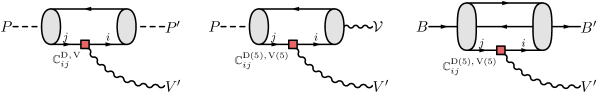
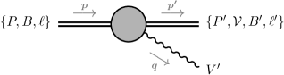
Figure 1 shows representative Feynman diagrams for the three types of decays.
Appendix E contains the analytical expressions for the corresponding decays rates (including the dependence on ); the relevant form factors are collected in Appendix E.1. Comparing the decay rates to the experimental upper limits on the branching ratios, we set upper bounds on the couplings in the basis333 In Appendix D we show the bounds in the basis. of Eq. (2.1) and Eq. (2.2), i.e. on the set , , , . The limits are determined as a function of the LDV mass, with range depending on the masses of the initial, , and final, , states of the decay at hand. Crucially, the form factors depend on the LDV mass and it is, therefore, essential to consider the full form-factor parametrization for an accurate analysis.
The available theoretical and experimental information is summarized in Table 1, where we collect the references for the form factors and relevant experimental limits. Often the experimental collaborations do not provide limits on two-body decays with missing energy. Yet, in some cases there is enough information to extract this bound from available data. We indicate this case by a subindex “” in the last column of the table, and either use existing recasts in the literature or perform our own recast, e.g., to find a bound on from BaBar data on the corresponding three-body decays [35, 36], see Appendix C for details.
Concretely we use our recast for only for LDV masses above . Note that we can recast only the experimental results of the BaBar collaboration and cannot use the newer Belle measurements, since the Belle collaboration does not provide the event count as a (binned) function of the missing-momentum distribution. We use existing recasts for decays from LEP [55, 56], decays from Belle II [57, 39] (this recast is limited to masses below ), decays from BaBar [57, 36] (below ). For invisible baryon decays for which there is no analysis, we derive limits using the total lifetime from the PDG [58] after subtracting all observed channels as in Ref. [22].
For the bound based on decays we use the result of Ref. [22] for , obtained from recasting CLEO data on [37]. We also perform a recast of these data for LDV masses up to (which is the upper range of the CLEO data set), assuming the efficiency in all bins to be the same as for . Note that recasting BES III data [59] on gives weaker constraints [22], although this result does not use the full experimental information. It would be interesting if BES III would provide an explicit two-body recast of their full data set. The collaboration actually does this for the case of two-body hyperon decays , albeit only for “massless” invisible particles. Their signal region in fact covers invisible masses up to , and leads to limits that are much stronger than the ones obtained by saturating the total lifetime [22]. As a conservative limit, to be replaced by a dedicated experimental analysis, we multiply their limit for the massless case by a factor 1/2 (since close to the endpoint of the signal region half of the signal events are lost due to energy resolution). We use the resulting bound for LDV masses up to , and take lifetime limits above . We notice that a search for the decay would not suffer from two-body SM backgrounds in contrast to hyperon decays, where contributes to the signal of a massless , if the photon is missed.
| Quark Transition | Hadronic Process | Form Factors | Experimental Limit |
| [60, 61] | NA62 [34, 33, 17] | ||
| [32, 62, 63, 64] | BES III [65], Lifetimer[58, 22] | ||
| [32, 62, 63, 64] | Lifetimer[58, 22] | ||
| [32, 62, 63, 64] | Lifetimer[58, 22] | ||
| [32, 62, 63, 64] | Lifetimer[58, 22] | ||
| [32, 62, 63, 64] | Lifetimer[58, 22] | ||
| [66, 66] | BaBarr [36], Belle IIr [57, 39] | ||
| [66, 66] | BaBarr [36, 57] | ||
| [67, 67] | Lifetimer[58, 22] | ||
| [68, 66] | BaBarr [35] | ||
| [66, 66] | LEPr [55, 56] | ||
| [67, 69] | Lifetimer [58, 22] | ||
| [70, 71] | CLEOr [37, 22] | ||
| [72, 72] | BES III [40], Lifetimer [58, 22] |
To set constraints on the couplings , , , we consider dipole () and vector interactions () separately, and turn on a single coupling at a time. We use the theory predictions in Appendix E together with the form factors in Table 1 (see also Appendix E.1) to calculate the decay rates as a function of the couplings and the LDV mass. The rates are then compared to the experimental limits to obtain the bounds in the mass–coupling plane. We include statistical and systematic uncertainties as follows. For the theory predictions we only use the systematic uncertainties associated with hadronic form factors (these are the most relevant ones), while the treatment of uncertainties of experimental limits depend on their nature: for decays where the experimental collaborations provide two-body interpretations (or a theory recast exists), we add the experimental and form-factor uncertainties in quadrature. In the case where we performed our own two-body recast (as described in Appendix C) we treat theory uncertainties as Gaussian uncertainties smearing the expectation values of the underlying Poisson probability distribution functions.
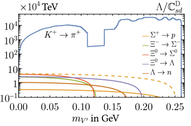
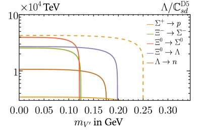
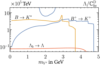
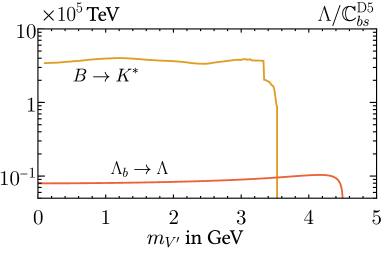
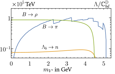
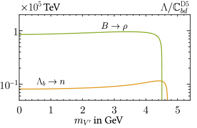
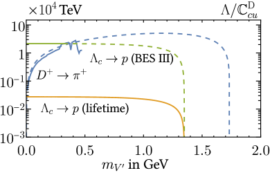
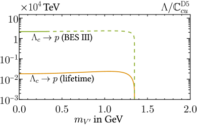
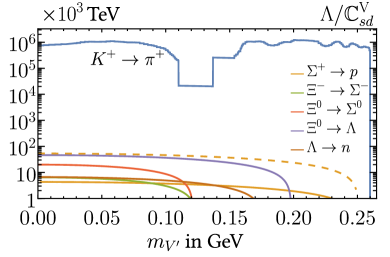
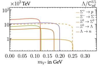
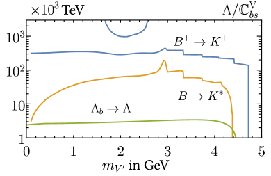
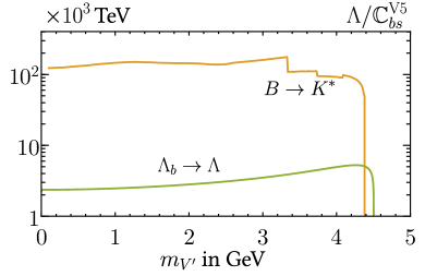
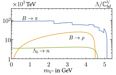
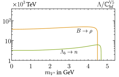
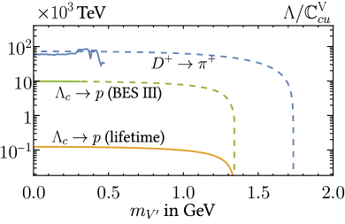
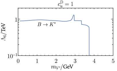
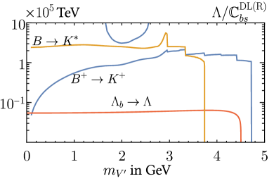
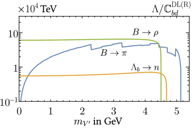
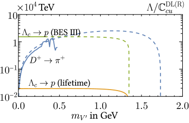
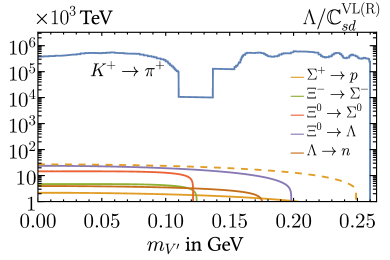
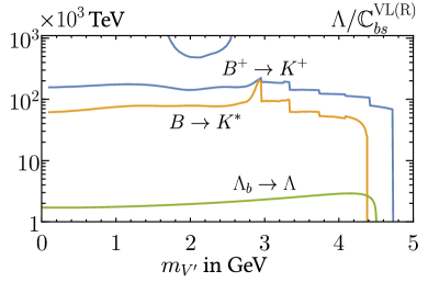
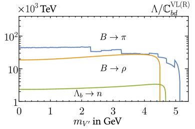
Our results are summarized in Figures 2 and 3 in which we show the lower bounds on the effective inverse coupling for given LDV mass . The plots are organized according to the underlying flavor transition, i.e, , , , and and we separate dipole , (Figure 2) and vector couplings , (Figure 3). Each plot shows the bound on a single coupling for a given quark-flavor transition, with each line corresponding to a particular hadronic decay, excluding the region below. Note that decays are only sensitive to and couplings, which follows from parity conservation of the strong interactions and the Lorentz structure of the form factors (see Appendix E.1). Also note that dipole operators are dimension-six above the electroweak scale, so in fact the actual UV scale probed is in all transitions.
3.1 Dark Dipole Interactions
Transitions
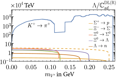
The bounds on the dipole couplings , are set by and hyperon decays, cf. Table 1 and Figure 2. For the two-body decay we use the bound provided by the NA62 collaboration [34]. For baryon decays there is an upper limit from BES III [65] on the decay with a massless invisible. We estimate the potential reach for this search by extending it to larger invisible masses by assuming that the same experimental limit is valid for the whole kinematic range. This is indicated by a dashed orange line. For all other baryon searches, we set upper limits on branching ratios indirectly as in Ref. [22] by subtracting the measured branching fractions for all relevant hyperon decay channels from unity. Due to this rather weak limit, sets a much more stringent constraint than hyperon decays, limiting the UV scale to be at least of the order . Note however that the search for strenghtens the upper limit by two orders of magnitude compared to the conservative limit estimated with the total lifetime, and thus, out of all baryon decays, it yields the strongest limit of order on the scale .
Nevertheless baryon decays with missing energy are important for two reasons. The decays to pseudoscalar, such as , are only sensitive to the , couplings. Thus baryon decays are crucial to constrain the axial coupling (of the order of a few ), as there are no two-body decays to vector particles in transitions. Moreover, the decay rates of pseudoscalar processes are proportional to the LDV mass for the dipole interaction (cf. Eq. (E.12)), and thus only baryon decays can constrain for small LDV masses. This can be see in Figure 2 (upper left panel), where the bounds on from hyperon decays dominate for LDV masses of yielding a limit of on the axial coupling . This provides a strong motivation for explicit direct searches targeting baryon decays with invisible final states.
Transitions
The limits on the dipole couplings are set by -meson decays and baryon decays . The limits from the -meson decays are obtained from our own recast of BaBar data (cf. Appendix C), except for for LDV masses where we use the recast in Ref. [57] of the recent Belle II measurement of [39]. We also use the recast in Ref. [57] of the BaBar measurement of [36] below LDV masses of 3 GeV. The limit on unobserved decays such as is obtained by comparing the SM prediction for the total lifetime with the experimental one inferred from all observed channels, ascribing the difference to the allowed value for the two-body invisible decay [22]. As for transitions, decays to pseudoscalar mesons such as can neither constrain the axial coupling , nor for very small LDV masses. Otherwise, however, they do dominate over the constraint from .
In contrast to transitions, there is also a decay with vector mesons in the final-state, , which constrains both the and the couplings in the entire LDV mass range, if kinematically allowed. Hence, decays are complementary to decays in constraining , setting limits on the UV scale of the order , and also dominate the bounds on of similar size, up to a small region where this channel is kinematically closed and decays set the strongest limit, of the order . Note that there is an upper limit of order on at around coming from decays [57], due to a excess in the latest Belle II measurement of [39].
Transitions
The bounds on the dipole couplings are obtained from -meson decays and baryon decays The limit on decays is obtained from our recast of BaBar data (cf. Appendix C), while a limit on decays from LEP data [55] has been derived in Ref. [56]. Analogously to transitions, the pseudoscalar decay does neither constrain the axial coupling nor for small LDV masses, while the decay to vector mesons does. Thus the two meson decays are complementary in setting limits on , of the order of , while dominates the bounds on the limits on of similar size, except for LDV masses above the kinematic threshold where decays take over, constraining UV scales up to .
Transitions
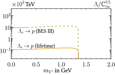
Finally, the constraints on the dipole couplings are set by and the baryonic process . For and LDV masses , we performed a recast of the CLEO data set (analogous to the -decay recasts in Appendix C). The result is shown as a solid, blue line in the bottom panel of Fig. 2. CLEO has only collected data up to masses of , but we also show the potential bound that could be obtained above this mass by extrapolating the bound for massless invisible particles [22] to the whole kinematic range, which we indicate by a dashed blue line.
For we show two limits in the bottom panel of Fig. 2: solid, orange lines denote the bound obtained from simply saturating the total lifetime, i.e., , while the green line indicates the 95% CL bound obtained from the BES III [40] result for “massless” invisible particles, at 90% CL, which in fact covers invisible masses up to and are multiplied by a factor 1/2, see the discussion in the beginning of this section. We estimate the potential reach for a search extending to larger invisible masses by assuming that the same experimental limit below is also valid above, and indicate this extrapolation by a dashed, green line. We observe that the strongest limits on are set by the BES III search for a “massless” LDV in decays, which are valid for and are of the order of . Between a limit of similar size is obtained from decays, recasting CLEO data on . The only available limit on LDV masses above arises from the total lifetime, which sets limits of order . Naively extrapolating the limits from CLEO on and BES III on decays to higher LDV masses instead suggests that present bounds could be strengthened by two orders of magnitude, if BES III would either analyze the available searches for decays with extended signal regions, or use available data on to set a limit on the two-body decay.
Currently only decays are capable to set constraints on the axial coupling , of the order of and for LDV masses above and below , respectively. Besides extending the search for to higher LDV masses, this also motivates dedicated searches for other processes such as or at current or future experiments.
3.2 Dark Vector Interactions
Transitions
The limits on the vector couplings , are shown in Figure 3. As for dipole couplings, the relevant constraints arise from and hyperon decays, see Table 1. Analogous to the dipole case, the limit from BES III on the decay for a massless invisible is tentatively assumed to be valid for the whole kinematic range. The limit on the scale is indicated by a dashed orange line. decays dominate the limits on , restricting UV scales up to , but cannot constrain the axial coupling , where hyperon decays set the only available bounds of the order of . All limits are non-vanishing when the LDV mass is taken to zero, which is due to the choice of the prefactor in linear in the LDV mass, see Eq. (2.2). This corresponds to the gauge-less limit where the longitudinal polarization of the LDV is essentially a Goldstone boson. With this scaling the flavor-violating decay is similar to the SM decay , which also remains finite in the gauge-less limit, since the top quark dominantly decays to the charged Goldstone Higgs, which couples only via Yukawas to the quarks. Different choices for the prefactor, corresponding to specific UV completions, would result in bounds that would vanish in the limit of massless LDVs, with a LDV mass dependence that can obtained by rescaling the limits presented here.
Transitions
The constraints on the vector couplings , are obtained from -meson decays and the baryonic decays sets the strongest constraint on of the order of , but cannot constrain the axial coupling . Here the dominant constraints are set by decays, also of the order of , apart from the region where this channel is kinematically closed and takes over and sets limits on the UV scales up to . Again there is an upper limit of order on at around coming from decays [57], due to a excess from the latest Belle II measurement of [39].
Transitions
The bounds on the vector couplings , arise from -meson decays and the baryonic decays . Analogously to transitions decay sets the strongest constraint on of the order of , while is limited to about the same values by decays, up to LDV masses at the kinematic threshold where decays dominate the bound of order .
Transitions
Finally, the bounds on the vector couplings , are set by the decays and Meson decays dominate the bound on of order , while only baryon decays can constrain the axial coupling at order and , using the total lifetime and the extrapolation of the BES III measurement, respectively, analogous to the dipole case. Again, it would be interesting if BES III could extend their search for to higher invisible masses, as this is expected to strengthen the present bound on the UV scale by two orders of magnitude.
4 Lepton Phenomenology of Light Dark Vectors
| LFV Transition | Experimental Limit |
|---|---|
| TWIST [41], Jodidior [73, 18] | |
| Belle II [38] | |
| Belle II [38] |
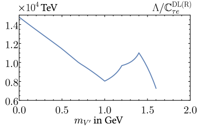
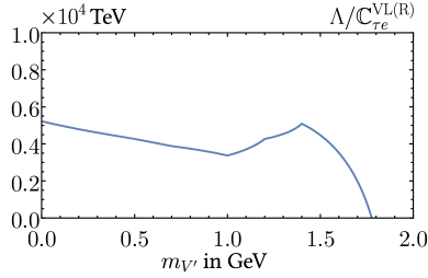
In this section we present the bounds on the flavor-violating couplings in Eq. (2.1) and (2.2) from LFV decays for lepton-flavor transitions , , and . There are three main differences to the quark-sector analysis: i) there is no hadronic input required, ii) the total decay rates only depend on the combination and , and iii) for the case of transitions one can profit from polarization in order to suppress SM background from Michel decays. This allows us to distinguish between and using the angular distribution of the outgoing electron.
Concretely, for we restrict the discussion to three benchmark scenarios, depending on the angular dependence of the differential two-body LFV decay rate in the limit of
| (4.1) |
where is the angle between the outgoing electron momentum and the muon polarization. We distinguish three benchmark cases: isotropic decays (), “” structure , and “” structure . Clearly polarization does not help to distinguish an LFV signal from the SM background for the SM case . Thus one can only rely on the monochromatic electron as the signal, which leads to weaker bounds than in the other cases [18]. Interestingly, many proposals have been put forward to look for this decay at present and future high-luminosity muon facilities [18, 19, 20, 21], which are sensitive also to invisible LDVs. We take present constraints on LFV transitions from the references indicated in Table 2, and compare them to the predictions for (polarized) lepton decay rates calculated in Appendix E.5.
Transitions
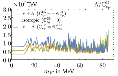
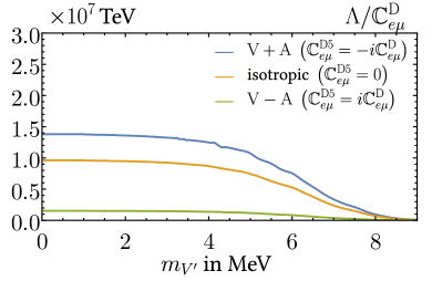
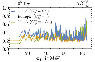
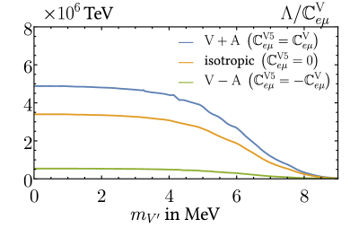
The bounds from decays on dipole and vector couplings are shown in Fig. 4. We derive them employing constraints from experiments conducted at TRIUMF, both by the TWIST collaboration [41] in 2015 (left panel) and Jodidio et al. [73] in 1986 (right panel). For the latter, we use the recast of Ref. [18]. The three curves in Fig. 4 show the bounds for the three benchmark scenarios for chiral structures, corresponding to or for , and for in the upper panel, while in the lower panel they correspond to or for , and for . For couplings that are not aligned to the SM, i.e., not “”, the dominant constraints on LDVs lighter than about 5 MeV are set by the Jodidio experiment, which limits UV scales of the order of . Heavier LDVs are constrained only by TWIST, setting limits of the order of few . LDVs with “” couplings are constrained by TWIST with bounds of the same order, exceeding the corresponding Jodidio limits also in the light-mass regime.
Transitions
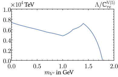
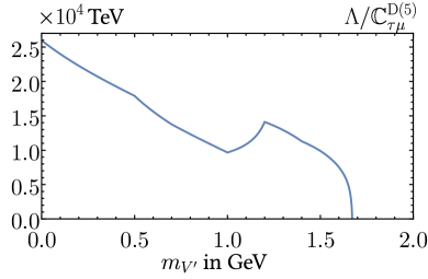
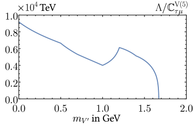
The limits from Belle II on decays constrain and transitions according to Fig. 5, where we shows the bounds on the dipole (left panel) and vector couplings (right panel). Constraints on the axial couplings and are at the same level, as the difference is suppressed by , cf. Appendix E.5. Bounds for and transitions are comparable, limiting UV scales of the order of few for dipole couplings, and few for vector couplings.

5 Flavor-violating LDVs from the Renormalization Group
In this section we study the phenomenologically interesting scenario in which LDV interactions with the SM are flavor-universal in the UV theory, so that flavor-violating couplings are generated only from the SM flavor violation via the renomalization-group evolution. We start right below the UV scale —taken to be much above the electroweak scale—and consider invariant vector and dipole interactions of the to the SM. For vector couplings see the trivial generalization of Eq. (2.3) and for dipole couplings see Eq. (2.6). We align possible new sources of flavor-violation of the with the flavor violation in the SM by taking the vector couplings to be flavor-universal, i.e., proportional to the identity matrix in flavor space, and by taking the dipole couplings to be proportional to the SM Yukawas. In both cases they are flavor diagonal in the mass basis, such that flavor-changing interactions with the are only induced by the renormalization-group evolution to the EW scale and always proportional to the CKM matrix. Flavor-violating couplings in the IR thus follow the paradigm of minimal flavor violation (MFV) [42].
We do not explicitly consider kinetic mixing between the LDV and the boson, as it leads only to a shift in the flavor-universal LDV couplings after diagonalising the photon kinetic terms. By working in this basis, our results also apply to models with kinetic mixing, upon re-defining the flavor-universal couplings.
5.1 Dipole interactions
In the interaction basis, the dipole interactions of the LDV with SM fermions are given by (cf. Eq. (2.6))
| (5.1) |
with the SM Yukawa matrices , , and arbitrary matrices . The one-loop RG equations for the couplings and the Yukawa matrices are listed in Appendix B. For the UV universal setup that we consider, the initial conditions at the UV scale are
| (5.2) |
with . By solving the RGE at leading-logarithmic accuracy and subsequently rotating to the mass basis for the quarks we find the low-energy dipole couplings in the notation of Eq. (2.3) with to be444 Since the couplings at the UV scale are aligned to the SM Yukawa matrices, a correction from the Yukawa RGE, given in Appendix B, must be included.
| (5.3) |
where is the CKM matrix, and are the diagonal SM Yukawas. The left-handed couplings are related to the ones in Eq. (5.3) by hermitian conjugation, . Note that indeed flavor off-diagonal entries are generated in both the up- and the down-quark sector at one-loop. They are proportional to the CKM matrix and the UV coupling of the other sector, i.e., and . Carrying out the matrix multiplications, one can identify the numerically leading contribution to a given flavor transition. We show these leading contributions in Table 3 for both sectors.
Using these results, we determine the experimental limits on the high-scale couplings and in Eq. (5.2) from the limits on two-body meson decays discussed in Section 3. Note that the renormalization scale is set to the EW scale since below there is no Yukawa running.
As expected from the high-level of flavor suppression inherent to the setup, the resulting bounds are very mild and often weaker than the constraints from perturbative unitarity. For this reason we only display in Fig. 6 (left panel) the strongest bounds, which come from and require for (for the limit on is far below the electroweak scale and is therefore not shown).
5.2 Vector interaction
In the interaction basis, the vector interactions of the LDV with the SM fermions are given by (cf. Eq. (2.3))
| (5.4) |
with SM Yukawa matrices , , and arbitrary hermitian matrices with . The one-loop RG equations for the couplings and the Yukawa matrices are listed in Appendix B. For the UV universal setup that we consider in this section, the boundary conditions at the UV scale are
| (5.5) |
with real numbers.
By solving the RGE at leading-logarithmic accuracy and subsequently rotating to the mass basis for the quarks, we find the low-energy vector couplings in the notation of Eq. (2.3) to be
| (5.6) |
where is the CKM matrix and are the diagonal SM Yukawas. Note that the couplings of right-handed interactions are always flavor diagonal, while flavor-violating terms in the IR are induced in the left-handed interactions , proportionally to and . Therefore, if the UV couplings are also universal among the different sectors, i.e., , there is no flavor violation in the IR at one-loop, as in this case the LDV actually couples to the baryon-number current, which is conserved at tree-level inducing flavor violation only at two-loop [74].
We now discuss this fact in more detail, before turning to the limits. One can rewrite the interactions in Eq. (5.4) for the case of flavor-universal UV boundary conditions in Eq. (5.5) in terms of the tree-level conserved (but anomalous) current , and the two non-conserved currents , and . As all currents are not conserved beyond tree-level, we take their coefficients to be proportional to the LDV mass
| (5.7) |
Matching to Eqs. (5.4) and (5.5) gives
| (5.8) |
At the one-loop level there is no flavor violation proportional to . However, flavor violation does arises due to the non-conserved currents and is thus proportional to the difference of couplings and . Rewriting Eq. (5.2) in terms of the UV coefficients with the proper LDV mass scaling gives finally
| (5.9) |
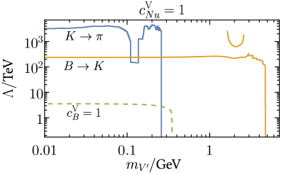
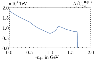
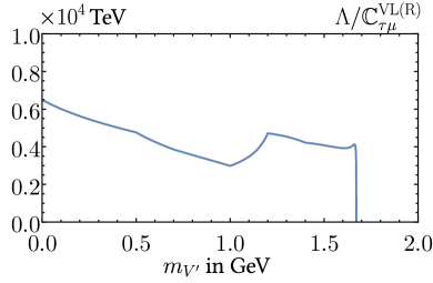
The numerically leading contributions to a given (hermitian) flavor transition in left-handed interactions are shown in Table 4 for both sectors. We display the resulting bounds on in the right panel of Fig. 6 for (there is no constraint from at one-loop), which are of order for transitions. These limits are weakened by about an order of magnitude for LDV masses above , where the dominant constraint comes from transitions. In dashed green, we also show the limits coming from the flavor-violating contribution that is induced at the two-loop level by the coupling of the LDV to the anomalous baryon current . The corresponding limit on the scale has been obtained by rescaling the result for of Fig. (1) from Ref. [74], giving for and . This is about three orders of magnitude weaker than the limit one obtains if the LDV also couples to currents that are not conserved at tree-level, i.e., taking .
6 Summary and Conclusions
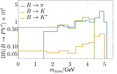
In this work we have systematically studied the flavor phenomenology of light dark vectors (LDVs). We have restricted our analysis to scenarios where the LDV is directly linked to dark matter, and is either itself invisible or promptly decays to invisible particles, such that the LDV appears as missing energy. Working in the context of a general EFT, we have considered both flavor-violating dipole (see Eq. (2.1)) and vector couplings (see Eq. (2.2)) of the LDV to SM fermions. We have calculated the resulting predictions for the decay rates of mesons, baryons, and polarized leptons as a function of the LDV mass, see Section E. These predictions were compared to the experimental limits on various hadronic processes (Table 1) and LFV transitions (Table 2). For decays experimental limits from B-factories are only available for three-body decays with two invisible neutrinos, so we have recasted available data to obtain bounds on the two-body decay with missing energy as a function of the LDV mass, see Fig. 7. The resulting limits on general vector and dipole interactions of the LDV are summarized in Figs. 2 and 3 for the quark sector, and in Fig. 4 and 5 for the lepton sector. Vector couplings are at least dimension-five operators, which results in very stringent limits on the UV scale, reaching up to in decays, in - and -meson decays, in decays, and in decays. Bounds on dipole couplings are weaker, if viewed as dimension-six operators above the EW scale, but they still probe UV scales of order in and decays. Importantly, all channels will be improved by present or near-future experiments, such as NA62, Belle II, BES III, MEG-II or Mu3e. We have also discussed a scenario where couplings in the UV are flavor-universal, so that quark-flavor violation is only induced radiatively through the CKM matrix. For this analysis we derived the relevant renormalization-group equations (RGEs) for both dipole and minimal couplings in Appendix B, and used our previous results to convert limits on flavor-changing interactions into limits on flavor-diagonal couplings, see Figure. 6.
To summarize, the aim of this work is to stress the importance of flavor-violating transitions for light, dark-matter searches, which is copiously produced in the lab as missing energy in decays of SM particles. Here we focused on the LDV as part of a dark sector, and showed that present constraints from precision flavor experiments already probe UV scales as large as . This underlines the important role of present and next-generation flavor factories in hunting down dark matter in the laboratory.
Acknowledgments
We would like to thank Adam Falkowski, Jorge Martin Camalich and Zhijun Li for useful discussions and Jure Zupan for comments on the manuscript. This work has received support from the European Union’s Horizon 2020 research and innovation programme under the Marie Skłodowska-Curie grant agreement No 860881-HIDDeN and is partially supported by project B3a and C3b of the DFG-funded Collaborative Research Center TRR257 “Particle Physics Phenomenology after the Higgs Discovery”.
Appendix A UV Motivation of Vector Couplings
In this section we motivate the scaling behavior of the flavor-violating vector coupling in the Lagrangian of Eq. (2.2), both by EFT considerations and explicit UV-complete models. In perturbative UV completions, the scaling is at least linear in the dark breaking scale, and we will provide two example scenarios: one that gives linear and one that gives quadratic scaling. We begin with the EFT discussion of the latter.
A.1 EFT Discussion for Quadratic scaling
For the EFT approach it is convenient to consider the coupling to the Goldstone boson in the gauge-less limit, rather than the coupling of the dark vector itself. They are related by the Goldstone-boson Equivalence Theorem, which states that at sufficiently high energies, or equivalently sufficiently small dark vector masses , the vector boson coupling is dominated by its longitudinal polarization, which in the small limit becomes the Goldstone boson. Thus one can work out the couplings of the Goldstone boson and recover the relevant vector-boson couplings by replacing in the interaction Lagrangian.
We, therefore, consider the case where the dark gauge group is spontaneously broken by some (SM singlet) scalar field with charge under the . We take the gauge-less limit, so that is a true Goldstone boson, contained in according to
| (A.1) |
where is the (real) VEV that breaks , connected to the dark vector mass by , and we have ignored the radial mode that obtains its mass around . This mode, together with all UV fields are taken to be much heavier than the electroweak scale, so that in the IR there is only the SM and the Goldstone boson , which is formally invariant under global transformations treating as a spurion with charge . Note that one can always realize such a scenario by making sufficiently small. Writing down the general EFT for this setup, it is clear that if SM fields are not charged under , the possible couplings of the Goldstone to SM fields must involve the same powers of and . The first such bilinear that gives a non-trivial combination containing the Goldstone is then . This implies that, e.g., right-handed down quarks can only couple to the Goldstone at the level of dimension-six operators only
| (A.2) |
where is the UV scale and in general there is flavor violation in the (hermitian) EFT coefficients, . The coupling of the dark vector in this setup is then recovered by , so is given by
| (A.3) |
This analysis demonstrates that the interactions of dark vectors with SM fields that are neutral under the scale at least as . In particular they involve an additional factor of the breaking scale as compared to Eq. (2.2). Below we will confirm this expectation in an explicit UV model, see Section A.3.
A.2 EFT Discussion for Linear scaling
In order to have dark-vector couplings with a linear scaling in the breaking scale, one necessarily has to charge SM fields under . In this case the vector boson couples directly to the charged fields via the dimension-four operator, e.g., for right-handed down quarks
| (A.4) |
where is the diagonal charge matrix. To see how off-diagonal entries are generated, one has to rotate to the mass basis, which is governed by the Yukawa couplings. It is clear that there is no flavor violation if is universal, i.e., proportional to the identity matrix. If instead charges are non-universal, the mass matrix cannot be generic at the renormalizable level, i.e., it does not yield realistic fermion masses without breaking . Therefore, insertions of or have to be considered to obtain realistic fermion masses.
Restricting for simplicity to two generations, and charging only with charge , i.e., , , the full Yukawa matrix requires higher-dimensional operators to have full rank
| (A.5) |
Thus the down-quark Yukawa matrix is given by
| (A.6) |
We can ignore here the Goldstone in , since we already have the coupling of the gauge field in Eq. (A.4), which leads to flavor-violating couplings with after rotating to the mass basis. Nevertheless we can also reproduce this coupling with the same arguments as above: in the gauge-less limit, we rescale , which removes from the Yukawa sectors. Ignoring chiral anomalies, this rescaling only affects the kinetic terms, as it is a local transformation
| (A.7) |
which reproduces Eq. (A.4) upon .
We are left to diagonalize the Yukawa matrix in Eq. (A.6), or rather , in order to find the mixing matrix of right-handed down quarks, defined as . In the limit when , one has
| (A.8) |
where we have set without loss of generality. Rotating the dark-vector couplings in Eq. (A.4) to the mass basis defined by gives finally
| (A.9) |
so that indeed off-diagonal couplings are generated proportional to .
To summarize, we have demonstrated that vector interactions of dark vectors can indeed be proportional to a single power of the breaking, and thus scale with the dark-vector mass as in Eq. (A.4), if SM fermions have non-universal charges. This situation is quite generic in models where SM Yukawa hierarchies are explained by non-anomalous abelian flavor symmetries, for example simple Froggatt-Nielsen models [51], see e.g. Refs. [7] for examples of such models without extra heavy fermions to cancel anomalies. It is well-known how to build UV completions for such models [75, 76], and below in Section A.4 we will present an illustrative example.
A.3 Explicit UV Model for Quadratic scaling
We first construct an explicit renormalizable model for the scaling of vector interactions in Eq. (2.2) quadratic in the dark breaking scale. We restrict the discussion for simplicity to the down-quark sector with two generations. The field content is summarized in Table 5, and is clearly anomaly-free.
The Lagrangian reads
| (A.10) |
with standard kinetic terms for all fields and
| (A.11) | ||||
| (A.12) | ||||
| (A.13) |
For a suitable choice of parameters, the last part in gives a vacuum expectation value to , , which sets the mass of the dark vector boson to
| (A.14) |
and induces a mixing between chiral quarks, , and vector-like fermions, , from the mixing term in . In the limit of we can integrate out the vector-like fermions using their equations of motion neglecting their kinetic terms
| (A.15) |
Plugging this back into kinetic terms and lead to the EFT
| (A.16) |
where . Next we integrate out the radial mode by substituting with the Goldstone parametrization in Eq. (A.1) and use the definition of the dark-vector mass to find
| (A.17) |
recovering the gauge-invariant555 In our conventions , , , . combination . Without loss of generality we can assume that is diagonal, so that we are already in the mass basis. Nevertheless, we do need to re-diagonalize the kinetic terms due to the second term in Eq. (A.17) induced in the EFT. In the limit of this is readily achieved by the rescaling . This leads to additional small corrections of to the final dark-vector couplings, which can be neglected, such that the leading couplings from the first term in Eq. (A.17) remain
| (A.18) |
These couplings are indeed quadratic in and are in general flavor violating, . This matches to the EFT term in Eq. (A.3) upon identifying .
A.4 Explicit UV Model for Linear scaling
We now construct an explicit renormalizable model for the minimal scaling of vector interactions in Eq. (2.2) proportional to a single power of the dark-vector mass. These types of models are motivated by scenarios addressing the SM flavor puzzle with non-anomalous abelian horizontal symmetries, see e.g. Ref. [7]. We restrict the discussion for simplicity to the down-quark sector with two generations. The field content is summarized in Table 6, and is not anomaly-free. However, we can always introduce further suitably charged chiral fermions in the right-handed up- and charged-lepton sector in order to cancel color and electromagnetic anomalies, respectively. Note that and carry the same quantum numbers.
The Lagrangian reads
| (A.19) |
with standard kinetic terms for all fields and
| (A.20) | ||||
| (A.21) | ||||
| (A.22) |
where we have simply defined to be that field having a mass term with . This already gives Eq. (A.4) and the first term in Eq. (A.5) from the EFT discussion, so it only remains to show that integrating out induces the second term in Eq. (A.5). The equations of motion for the heavy fermions read, neglecting kinetic terms
| (A.23) |
and, therefore, the resulting EFT Lagrangian term is
| (A.24) |
This indeed reproduces Eq. (A.5) with the identification of the UV scale as . The remaining calculation follows the EFT discussion, which shows that in these type of UV models the flavor violating couplings to scale indeed linearly with .
Appendix B Renormalization Group Equations
In this appendix we collect our results for the renormalization group equations relevant for the interactions of the LDV with SM quarks as discussed in Section 5. Since in the current work we focused on the case of the UV universal scenario, in which flavor-violation originates only from the SM CKM matrix, we present here only the one-loop RGEs proportional to Yukawa couplings. However, in what follows the matrices , , , and are generic matrices in flavor space, i.e., we have not assumed any alignment with the SM Yukawas. The relevant terms in the Lagrangian are the SM Yukawa interaction, the dipole, and the vector interactions with the LDV. They respectively read:
| (B.1) | ||||
| (B.2) | ||||
| (B.3) |
The one-loop RGEs for Yukawa running read [77]
| (B.4) |
with denoting the number of colors. The one-loop running of the Yukawas is relevant for the dipole analysis because the RG-evolved Yukawas contribute to the flavor-violating couplings upon rotation to the quark mass-eigenstates at the EW scale [78].
For the one-loop RGE of the dipole couplings proportional to the SM Yukawas we find
| (B.5) |
For the one-loop RGE of the vector couplings proportional to the SM Yukawas we find
| (B.6) |
Appendix C Recast of Experimental Limits
Experimental collaborations often provide only limits on the branching ratios in terms of the three body decay , as a function of the squared invariant mass of the di-neutrino system . In order to get the experimental limits on the two body decays , we use the event count per -bin information, if provided by the experimental collaborations. Only the BaBar experiment [35, 36] provides all information needed to perform a recast for two-body decays . For and dark-vector masses , we use the sophisticated recast of Ref. [57], otherwise we estimate upper limits on the Wilson coefficients in terms of the CL method as explained below.
For a given Wilson coefficient , the number of signal events in a -bin is given as
| (C.1) |
where is the total number of mesons and the efficiency associated to bin . Further, denotes the branching ratio of within the -bin . The likelihood is then given as a Poisson distribution in the number of signal plus background events. The efficiency and total number of mesons are included as global observables associated to auxiliary measurements. The uncertainty on the signal, assumed to be Gaussian, is given by the NP theoretical prediction and is dominated by the form-factor uncertainty. The systematic uncertainty on the background is implemented as a Gaussian distribution. With this in mind, we denote the likelihood as with being the outcome, i.e., the observed data, the parameter of interest, i.e., the Wilson coefficient, and the nuisance parameters. As a test statistics , we choose a one-sided profile likelihood. Note that the parameter of interest is actually since the branching ratio only depends on as we only consider one coupling at a time. The -value of the hypothesis for a given value of the Wilson coefficient is then given by
| (C.2) |
where denotes the value of the test statistics for the observed data, denotes the pdf of the test statistics , and are the values of the nuisance parameter that maximise the likelihood for a given . The CL limit on the Wilson coefficient is then given by the value of such that
| (C.3) |
where denotes the -value of the background only hypothesis. In order to evaluate Eq. (C.2), one needs the pdf of the test statistics for which we use the ROOT toolkit RooStats in order to sample the distribution by means of a Monte Carlo method.
Taking the as a parameter of interest instead of the Wilson coefficient , we can determine a model independent limit on the two body branching ratios, see Figure 7.
Appendix D Limits in the Basis
In this appendix we present bounds on the couplings in the basis , , , , which are obtained from the limits in the basis (discussed in Section 3 and 4)) using Eq. (2.4). As the decay rates are symmetric with respect to the bounds on both couplings are the same.
D.1 Quark Dipole Interactions
D.2 Quark Vector Interactions

Appendix E Two-body decays to Light Dark Vectors
In this appendix we present the full expressions for the two-body decays to a LDV that enter our analysis, namely
-
•
: pseudoscalar meson to pseudoscalar meson and LDV,
-
•
: pseudoscalar meson to vector meson and LDV,
-
•
: baryon to baryon and LDV,
-
•
: lepton to lepton and LDV.
For the hadronic processes illustrative Feynman diagrams are shown in Figure 1, while throughout this appendix we define the two-body kinematics for all decays as in Figure 11, namely as
| (E.1) |
with and . In the next subsection we collect the parametrization of all the relevant form factors for the hadronic processes considered, and in the subsequent subsections we present the expressions for the rates. The numerical values for the form-factors are always taken from the most recent work referenced.
E.1 Form Factors
For the pseudoscalar decays to two vectors with denoting the vector-meson, the hadronic matrix element for the vector and axial-vector currents are parametrized as [66]
| (E.4) |
where denotes the polarization of . The kinematic functions read
| (E.5) |
where denotes the polarization vector of the outgoing . The scalar form factors can be further parametrized as
| (E.6) | ||||
with , which ensures finite matrix elements at , i.e., for massless LDV.
The corresponding matrix elements for tensor and pseudo-tensor currents read [66]
| (E.7) |
where
| (E.8) |
For vanishing momentum transfer , i.e., massless LDV, the scalar form-factors satisfy
| (E.9) |
while the contribution proportional to vanishes.
For the baryon decays the matrix elements for vector and axial-vector currents are parametrized by [67, 69, 72]
| (E.10) |
with and the spinor functions for and respectively. For decays the values of the form factors are taken from [67, 69, 72], while for hyperon decays they are taken from [62, 63, 64].
The corresponding matrix elements for tensor and pseudo-tensor currents have the form [32, 79]
| (E.11) |
which is an approximation valid for , which we use for the hyperon decays. For the baryon , , and decays we use the available full parametrization, given by [67, 72]
Having collected all hadronic input used in the analysis we next present the full expressions for the two-body rates. We show separately the contributions from dipole and vector interactions with the LDV, c.f. Eqs. (2.1) and (2.2). For brevity we drop the argument in all form factors since it is always in two-body decays. To shorten the expression we also introduce the notations
with indicating the mass of the final-state particle and the mass of the decaying particle.
E.2 Partial width for
The partial width for the decay with an underlying flavor-changing transition is given respectively for dipole and vector interaction by
| (E.12) | ||||
| (E.13) |
Note that due to the parity conservation of strong interactions the rate is independent of the axial couplings and . Therefore, decays are only sensitive to the couplings. In the basis, these decays are sensitive to both couplings.
In the limit for massless LDV, the leading in contributions to the decay rates read
| (E.14) | ||||
| (E.15) |
While the rate originating from dipole interactions vanishes in the massless limit, the contribution of the vector interaction remains constant due to the linear scaling introduced and discussed in Eq. (2.2).
E.3 Partial width for
The partial width for the decay with an underlying flavor-changing transition is given respectively for dipole and vector interaction by
| (E.16) | ||||
with the coefficients given by
| (E.17) | ||||
| (E.18) | ||||
| (E.19) | ||||
| (E.20) |
In the limit of a massless LDV, the decay rates reduce to
| (E.21) |
which illustrates that the sensitivity to weakens for very light LDVs.
E.4 Partial width for
For baryon decays with an underlying transition the contribution to the partial width from the dipole and vector interaction read
| (E.22) | ||||
with the kinematic coefficients
In the limit of a massless LDV, the rates reduce to
| (E.23) | ||||
For hyperon decays we use the form factor parametrization of Eq. (E.11), valid for . Nonetheless, we consider a massive LDV for the kinematics for completeness. The decay rate reads
| (E.24) | ||||
with the kinematic coefficients
| (E.25) |
In the limit of a massless LDV, the rate reduces to
| (E.26) | ||||
For a fully polarized initial , the differential width read
| (E.27) | ||||
with the kinematic coefficients
| (E.28) | ||||||||
| (E.29) |
In the limit of a massless LDV, the rate reduces to
| (E.30) | ||||
E.5 Polarized lepton distributions and rates
Next we consider the decays for the case in which lepton-flavor violating dipole or vector interactions with the LDV are present. In this case there is experimental sensitivity to the polarization of the initial lepton by the measurement of the angular distribution of the angle , defined as the angle between the polarization vector of and the three-momentum of . For the different LDV interactions we find for the differential width of a fully polarized initial
| (E.31) |
with the kinematic coefficients
| (E.32) | ||||||
In the limit of massless LDV, the polarized differential two-body rate reduces to
| (E.33) |
Finally, after integrating over and averaging over the initial- and final-state polarizations, the total decay rates read
| (E.34) | ||||
| (E.35) |
which in the limit of massless LDVs reduces to
| (E.36) |
References
- [1] S. Knapen, T. Lin and K.M. Zurek, Light Dark Matter: Models and Constraints, Phys. Rev. D 96 (2017) 115021 [1709.07882].
- [2] B. Holdom, Two U(1)’s and Epsilon Charge Shifts, Phys. Lett. B 166 (1986) 196.
- [3] B.A. Dobrescu, Massless gauge bosons other than the photon, Phys. Rev. Lett. 94 (2005) 151802 [hep-ph/0411004].
- [4] T. Hambye, M.H.G. Tytgat, J. Vandecasteele and L. Vanderheyden, Dark matter from dark photons: a taxonomy of dark matter production, Phys. Rev. D 100 (2019) 095018 [1908.09864].
- [5] E.J. Chun, J.-C. Park and S. Scopel, Dark matter and a new gauge boson through kinetic mixing, JHEP 02 (2011) 100 [1011.3300].
- [6] M. Fabbrichesi, E. Gabrielli and G. Lanfranchi, The Dark Photon, 2005.01515.
- [7] B.C. Allanach, J. Davighi and S. Melville, An Anomaly-free Atlas: charting the space of flavour-dependent gauged extensions of the Standard Model, JHEP 02 (2019) 082 [1812.04602].
- [8] M. Williams, C.P. Burgess, A. Maharana and F. Quevedo, New Constraints (and Motivations) for Abelian Gauge Bosons in the MeV-TeV Mass Range, JHEP 08 (2011) 106 [1103.4556].
- [9] A. Smolkovič, M. Tammaro and J. Zupan, Anomaly free Froggatt-Nielsen models of flavor, JHEP 10 (2019) 188 [1907.10063].
- [10] Y. Kahn, G. Krnjaic, S. Mishra-Sharma and T.M.P. Tait, Light Weakly Coupled Axial Forces: Models, Constraints, and Projections, JHEP 05 (2017) 002 [1609.09072].
- [11] M. Bauer, P. Foldenauer and J. Jaeckel, Hunting All the Hidden Photons, JHEP 07 (2018) 094 [1803.05466].
- [12] A. Greljo, P. Stangl, A.E. Thomsen and J. Zupan, On (g 2)μ from gauged U(1)X, JHEP 07 (2022) 098 [2203.13731].
- [13] R. Bause, H. Gisbert, G. Hiller, T. Höhne, D.F. Litim and T. Steudtner, U-spin-CP anomaly in charm, Phys. Rev. D 108 (2023) 035005 [2210.16330].
- [14] J. Brod, J. Drobnak, A.L. Kagan, E. Stamou and J. Zupan, Stealth QCD-like strong interactions and the asymmetry, Phys. Rev. D 91 (2015) 095009 [1407.8188].
- [15] A. Badin and A.A. Petrov, Searching for light Dark Matter in heavy meson decays, Phys. Rev. D 82 (2010) 034005 [1005.1277].
- [16] J.F. Kamenik and C. Smith, FCNC portals to the dark sector, JHEP 03 (2012) 090 [1111.6402].
- [17] E. Goudzovski et al., New physics searches at kaon and hyperon factories, Rept. Prog. Phys. 86 (2023) 016201 [2201.07805].
- [18] L. Calibbi, D. Redigolo, R. Ziegler and J. Zupan, Looking forward to lepton-flavor-violating ALPs, JHEP 09 (2021) 173 [2006.04795].
- [19] Y. Jho, S. Knapen and D. Redigolo, Lepton-flavor violating axions at MEG II, JHEP 10 (2022) 029 [2203.11222].
- [20] S. Knapen, K. Langhoff, T. Opferkuch and D. Redigolo, A Robust Search for Lepton Flavour Violating Axions at Mu3e, 2311.17915.
- [21] R.J. Hill, R. Plestid and J. Zupan, Searching for new physics at facilities with and decays at rest, 2310.00043.
- [22] J. Martin Camalich, M. Pospelov, P.N.H. Vuong, R. Ziegler and J. Zupan, Quark Flavor Phenomenology of the QCD Axion, Phys. Rev. D 102 (2020) 015023 [2002.04623].
- [23] J.L. Feng, T. Moroi, H. Murayama and E. Schnapka, Third generation familons, B factories, and neutrino cosmology, Phys. Rev. D 57 (1998) 5875 [hep-ph/9709411].
- [24] F. Björkeroth, E.J. Chun and S.F. King, Flavourful Axion Phenomenology, JHEP 08 (2018) 117 [1806.00660].
- [25] R. Ziegler, Flavor Probes of Axion Dark Matter, PoS DISCRETE2022 (2024) 086 [2303.13353].
- [26] L.D. Landau, On the angular momentum of a system of two photons, Dokl. Akad. Nauk SSSR 60 (1948) 207.
- [27] C.-N. Yang, Selection Rules for the Dematerialization of a Particle Into Two Photons, Phys. Rev. 77 (1950) 242.
- [28] E. Gabrielli, B. Mele, M. Raidal and E. Venturini, FCNC decays of standard model fermions into a dark photon, Phys. Rev. D 94 (2016) 115013 [1607.05928].
- [29] M. Fabbrichesi, E. Gabrielli and B. Mele, Hunting down massless dark photons in kaon physics, Phys. Rev. Lett. 119 (2017) 031801 [1705.03470].
- [30] J.-Y. Su and J. Tandean, Searching for dark photons in hyperon decays, Phys. Rev. D 101 (2020) 035044 [1911.13301].
- [31] J.-Y. Su and J. Tandean, Kaon decays shedding light on massless dark photons, Eur. Phys. J. C 80 (2020) 824 [2006.05985].
- [32] J.M. Camalich, J. Terol-Calvo, L. Tolos and R. Ziegler, Supernova Constraints on Dark Flavored Sectors, Phys. Rev. D 103 (2021) L121301 [2012.11632].
- [33] NA62 collaboration, Search for decays to invisible particles, JHEP 02 (2021) 201 [2010.07644].
- [34] NA62 collaboration, Measurement of the very rare K+→ decay, JHEP 06 (2021) 093 [2103.15389].
- [35] BaBar collaboration, A search for the decay , Phys. Rev. Lett. 94 (2005) 101801 [hep-ex/0411061].
- [36] BaBar collaboration, Search for and invisible quarkonium decays, Phys. Rev. D 87 (2013) 112005 [1303.7465].
- [37] CLEO collaboration, Precision Measurement of B( ) and the Pseudoscalar Decay Constant , Phys. Rev. D 78 (2008) 052003 [0806.2112].
- [38] Belle-II collaboration, Search for lepton-flavor-violating decays to a lepton and an invisible boson at Belle II, 2212.03634.
- [39] Belle-II collaboration, Evidence for Decays, 2311.14647.
- [40] BESIII collaboration, Search for a massless dark photon in →p’ decay, Phys. Rev. D 106 (2022) 072008 [2208.04496].
- [41] TWIST collaboration, Search for two body muon decay signals, Phys. Rev. D 91 (2015) 052020 [1409.0638].
- [42] G. D’Ambrosio, G.F. Giudice, G. Isidori and A. Strumia, Minimal flavor violation: An Effective field theory approach, Nucl. Phys. B 645 (2002) 155 [hep-ph/0207036].
- [43] G. Isidori and D.M. Straub, Minimal Flavour Violation and Beyond, Eur. Phys. J. C 72 (2012) 2103 [1202.0464].
- [44] H. Ruegg and M. Ruiz-Altaba, The Stueckelberg field, Int. J. Mod. Phys. A 19 (2004) 3265 [hep-th/0304245].
- [45] B. Kors and P. Nath, A Stueckelberg extension of the standard model, Phys. Lett. B 586 (2004) 366 [hep-ph/0402047].
- [46] B. Kors and P. Nath, Aspects of the Stueckelberg extension, JHEP 07 (2005) 069 [hep-ph/0503208].
- [47] A. DiFranzo, P.J. Fox and T.M.P. Tait, Vector Dark Matter through a Radiative Higgs Portal, JHEP 04 (2016) 135 [1512.06853].
- [48] M. Zaazoua, L. Truong, K.A. Assamagan and F. Fassi, Higgs Portal Vector Dark Matter Interpretation: Review of Effective Field Theory Approach and Ultraviolet Complete Models, LHEP 2022 (2022) 270 [2107.01252].
- [49] S. Baek, P. Ko and W.-I. Park, Addendum to ”Invisible Higgs decay width versus dark matter direct detection cross section in Higgs portal dark matter models”, Phys. Rev. D 105 (2022) 015007 [2112.11983].
- [50] G. Arcadi, J.C. Criado and A. Djouadi, Iteration on the Higgs-portal for vector Dark Matter and its effective field theory description, 2312.14052.
- [51] C.D. Froggatt and H.B. Nielsen, Hierarchy of Quark Masses, Cabibbo Angles and CP Violation, Nucl. Phys. B 147 (1979) 277.
- [52] D. Barducci, M. Nardecchia and C. Toni, Perturbative unitarity constraints on generic vector interactions, 2306.11533.
- [53] J. Folch Eguren, E. Stamou, M. Tabet and R. Ziegler, to appear, .
- [54] J. Albrecht, E. Stamou, R. Ziegler and R. Zwicky, Flavoured axions in the tail of Bq → +- and B → ∗ form factors, JHEP 21 (2020) 139 [1911.05018].
- [55] ALEPH collaboration, Measurements of BR ( ) and BR ( ) and upper limits on BR ( ) and BR ( ), Eur. Phys. J. C 19 (2001) 213 [hep-ex/0010022].
- [56] G. Alonso-Álvarez and M. Escudero, The first limit on invisible decays of mesons comes from LEP, 2310.13043.
- [57] W. Altmannshofer, A. Crivellin, H. Haigh, G. Inguglia and J. Martin Camalich, Light New Physics in ?, 2311.14629.
- [58] Particle Data Group collaboration, Review of Particle Physics, PTEP 2022 (2022) 083C01.
- [59] BESIII collaboration, Search for the decay , Phys. Rev. D 105 (2022) L071102 [2112.14236].
- [60] I. Baum, V. Lubicz, G. Martinelli, L. Orifici and S. Simula, Matrix elements of the electromagnetic operator between kaon and pion states, Phys. Rev. D 84 (2011) 074503 [1108.1021].
- [61] ETM collaboration, K Semileptonic Form Factors from Two-Flavor Lattice QCD, Phys. Rev. D 80 (2009) 111502 [0906.4728].
- [62] T. Ledwig, J. Martin Camalich, L.S. Geng and M.J. Vicente Vacas, Octet-baryon axial-vector charges and SU(3)-breaking effects in the semileptonic hyperon decays, Phys. Rev. D 90 (2014) 054502 [1405.5456].
- [63] N. Cabibbo, E.C. Swallow and R. Winston, Semileptonic hyperon decays, Ann. Rev. Nucl. Part. Sci. 53 (2003) 39 [hep-ph/0307298].
- [64] J.M. Gaillard and G. Sauvage, HYPERON BETA DECAYS, Ann. Rev. Nucl. Part. Sci. 34 (1984) 351.
- [65] BESIII collaboration, Search for a massless particle beyond the Standard Model in the decay, 2312.17063.
- [66] N. Gubernari, A. Kokulu and D. van Dyk, and Form Factors from -Meson Light-Cone Sum Rules beyond Leading Twist, JHEP 01 (2019) 150 [1811.00983].
- [67] W. Detmold and S. Meinel, form factors, differential branching fraction, and angular observables from lattice QCD with relativistic quarks, Phys. Rev. D 93 (2016) 074501 [1602.01399].
- [68] D. Leljak, B. Melić and D. van Dyk, The → form factors from QCD and their impact on |Vub|, JHEP 07 (2021) 036 [2102.07233].
- [69] W. Detmold, C. Lehner and S. Meinel, and form factors from lattice QCD with relativistic heavy quarks, Phys. Rev. D 92 (2015) 034503 [1503.01421].
- [70] ETM collaboration, Tensor form factor of and decays with twisted-mass fermions, Phys. Rev. D 98 (2018) 014516 [1803.04807].
- [71] ETM collaboration, Scalar and vector form factors of decays with twisted fermions, Phys. Rev. D 96 (2017) 054514 [1706.03017].
- [72] S. Meinel, form factors from lattice QCD and phenomenology of and decays, Phys. Rev. D 97 (2018) 034511 [1712.05783].
- [73] A. Jodidio et al., Search for Right-Handed Currents in Muon Decay, Phys. Rev. D 34 (1986) 1967.
- [74] J.A. Dror, R. Lasenby and M. Pospelov, Dark forces coupled to nonconserved currents, Phys. Rev. D 96 (2017) 075036 [1707.01503].
- [75] M. Leurer, Y. Nir and N. Seiberg, Mass matrix models, Nucl. Phys. B 398 (1993) 319 [hep-ph/9212278].
- [76] L. Calibbi, Z. Lalak, S. Pokorski and R. Ziegler, The Messenger Sector of SUSY Flavour Models and Radiative Breaking of Flavour Universality, JHEP 06 (2012) 018 [1203.1489].
- [77] E.E. Jenkins, A.V. Manohar and M. Trott, Renormalization Group Evolution of the Standard Model Dimension Six Operators II: Yukawa Dependence, JHEP 01 (2014) 035 [1310.4838].
- [78] J. Aebischer and J. Kumar, Flavour violating effects of Yukawa running in SMEFT, JHEP 09 (2020) 187 [2005.12283].
- [79] R. Gupta, B. Yoon, T. Bhattacharya, V. Cirigliano, Y.-C. Jang and H.-W. Lin, Flavor diagonal tensor charges of the nucleon from (2+1+1)-flavor lattice QCD, Phys. Rev. D 98 (2018) 091501 [1808.07597].