From Linear to Linearizable Optimization: A Novel Framework with Applications to Stationary and Non-stationary DR-submodular Optimization

Abstract

This paper introduces the notion of upper linearizable/quadratizable functions, a class that extends concavity and DR-submodularity in various settings, including monotone and non-monotone cases over different convex sets. A general meta-algorithm is devised to convert algorithms for linear/quadratic maximization into ones that optimize upper quadratizable functions, offering a unified approach to tackling concave and DR-submodular optimization problems. The paper extends these results to multiple feedback settings, facilitating conversions between semi-bandit/first-order feedback and bandit/zeroth-order feedback, as well as between first/zeroth-order feedback and semi-bandit/bandit feedback. Leveraging this framework, new algorithms are derived using existing results as base algorithms for convex optimization, improving upon state-of-the-art results in various cases. Dynamic and adaptive regret guarantees are obtained for DR-submodular maximization, marking the first algorithms to achieve such guarantees in these settings. Notably, the paper achieves these advancements with fewer assumptions compared to existing state-of-the-art results, underscoring its broad applicability and theoretical contributions to non-convex optimization.

1 Introduction

Overview: The prominence of optimizing continuous adversarial $\gamma$-weakly up-concave functions (with DR-submodular and concave functions as special cases) has surged in recent years, marking a crucial subset within the realm of non-convex optimization challenges, particularly in the forefront of machine learning and statistics. This problem has numerous real-world applications, such as revenue maximization, mean-field inference, recommendation systems [4, 19, 29, 11, 23, 17, 25]. This problem is modeled as a repeated game between an optimizer and an adversary. In each round, the optimizer selects an action, and the adversary chooses a $\gamma$-weakly up-concave reward function. Depending on the scenario, the optimizer can then query this reward function either at any arbitrary point within the domain (called full information feedback) or specifically at the chosen action (called semi-bandit/bandit feedback), where the feedback can be noisy/deterministic. The performance metric of the algorithm is measured with multiple regret notions - static adversarial regret, dynamic regret, and adaptive regret. The algorithms for the problem are separated into the ones that use a projection operator to project the point to the closest point in the domain, and the projection-free methods that replace the projection with an alternative such as Linear Optimization Oracles (LOO) or Separation Oracles (SO). This interactive framework introduces a range of significant challenges, influenced by the characteristics of the up-concave function (monotone/non-monotone), the constraints imposed, the nature of the queries, projection-free/projection-based algorithms, and the different regret definitions.

Table 1: Online up-concave maximization

$F$	Set	Feedback			Reference	Appx.	# of queries	$\log_{T}(\alpha\text{-regret})$
Monotone	$0\in{\mathcal{K}}$	$\nabla F$	Full Information	stoch.	[45] $\ddagger$	$1-e^{-\gamma}$	$1$	$1/2$
					[34]	$1-e^{-1}$	$T^{\theta}(\theta\in[0,1/2])$	$2/3-\theta/3$
					Corollary 6-c	$1-e^{-\gamma}$	$1$	$1/2$
			Semi-bandit	stoch.	[34]	$1-e^{-1}$	-	$3/4$
					Corollary 6-c	$1-e^{-\gamma}$	-	$2/3$
		$F$	Full Information	stoch.	[34]	$1-e^{-1}$	$T^{\theta}(\theta\in[0,1/4])$	$4/5-\theta/5$
					Corollary 6-c	$1-e^{-\gamma}$	-	$3/4$
			Bandit	det.	[38] $\ddagger\ddagger$	$1-e^{-1}$	-	$3/4$
					[47] $\ddagger$	$1-e^{-\gamma}$	-	$4/5$
				stoch.	[34]	$1-e^{-1}$	-	$5/6$
					Corollary 6-c	$1-e^{-\gamma}$	-	$4/5$
	general	$\nabla F$	Full Information	stoch.	[34]	$1/2$	$T^{\theta}(\theta\in[0,1/2])$	$2/3-\theta/3$
			Semi-bandit	stoch.	[7]$\ddagger$	$\gamma^{2}/(1+\gamma^{2})$	-	$1/2$
					[34]	$1/2$	-	$3/4$
					Corollary 6-b	$\gamma^{2}/(1+c\gamma^{2})$	-	$1/2$
		$F$	Full Information	stoch.	[34]	$1/2$	$T^{\theta}(\theta\in[0,1/4])$	$4/5-\theta/5$
			Bandit	stoch.	[34]	$1/2$	-	$5/6$
					Corollary 6-b	$\gamma^{2}/(1+c\gamma^{2})$	-	$3/4$
Non-Monotone	general	$\nabla F$	Full Information	stoch.	[34]	$(1-h)/4$	$T^{\theta}(\theta\in[0,1/2])$	$2/3-\theta/3$
					[47] $\ddagger$	$(1-h)/4$	$1$	$1/2$
					Corollary 6-d	$(1-h)/4$	$1$	$1/2$
			Semi-bandit	stoch.	[34]	$(1-h)/4$	-	$3/4$
					Corollary 6-d	$(1-h)/4$	-	$2/3$
		$F$	Full Information	stoch.	[34]	$(1-h)/4$	$T^{\theta}(\theta\in[0,1/4])$	$4/5-\theta/5$
					Corollary 6-d	$(1-h)/4$	$1$	$3/4$
			Bandit	det.	[47] $\ddagger$	$(1-h)/4$	-	$4/5$
				stoch.	[34]	$(1-h)/4$	-	$5/6$
					Corollary 6-d	$(1-h)/4$	-	$4/5$

This table compares different static regret results for the online up-concave maximization. The logarithmic terms in regret are ignored. Here $h\mathrel{\mathop{\mathchar 58\relax}}=\min_{{\mathbf{z}}\in{\mathcal{K}}}\|{\mathbf{z}}\|_{\infty}$. Our algorithm is projection-free and use a separation oracle. The rows marked with $\ddagger$ use gradient ascent, requiring potentially computationally expensive projections. Note that the result of [38], marked by $\ddagger\ddagger$, uses a convex optimization subroutine in each iteration, which could potentially be more expensive than projection and therefore not considered a projection-free result. It is also the only existing result, in all the tables, that outperforms ours.

All results assume that functions are Lipschitz. Except for our results on monotone functions over general convex sets, all results also assume differentiability. All previous results assume that functions are DR-submodular, while we only require up-concavity. Results of [34] and [38] also assume functions are smooth, i.e., their gradients are Lipschitz.

In this paper, we present a comprehensive approach to solving adversarial up-concave optimization problems, encompassing different feedback types (including bandit, semi-bandit and full-information feedback), characteristics of the up-concave function and constraint region, projection-free/projection-based algorithms, and regret definitions. While the problem has been studied in many special cases, the main contribution of this work is a framework that is based on a novel notion of the function class being upper linearizable (or upper quadratizable). We design a meta-algorithm that converts certain algorithms designed for online linear maximization to algorithms capable of handling upper linearizable function classes. This allows us to reduce the problem of up-concave maximization in three different settings to online linear maximization and obtain corresponding regret bounds. In particular, our results include monotone $\gamma$-weakly up-concave functions over general convex set, monotone $\gamma$-weakly up-concave functions over convex sets containing the origin and non-monotone up-concave functions. While the above result is for first order feedback, we then derive multiple results that increase the applicability of the above results. We extend the applicability of $\operatorname{FOTZO}$ and $\operatorname{STB}$ algorithm introduced in [33] to our setting which allows us to convert algorithms for first-order/semi-bandit feedback into algorithms for zeroth-order/bandit feedback. We also design a meta-algorithm that allows us to convert algorithms that require full-information feedback into algorithms that only require semi-bandit/bandit feedback.

We demonstrate the usefulness of results through two applications as described in the following. In the first application, we use the SO-OGD Algorithm in [16] as the base algorithm for online linear optimization, which is a projection-free algorithm. Using this, we first obtain the adaptive regret (and therefore also static regret) guarantees for the three setups of DR-submodular (or more generally, up-concave) optimization with semi-bandit feedback/first order feedback in the respective cases. Then, the meta-algorithms for conversion of first-order/semi-bandit to zeroth-order/bandit are used to get result with zeroth-order/bandit feedback. In the cases where the algorithms are full-information and not (semi-)bandit, we use another meta-algorithm to obtain algorithms in (semi-)bandit feedback setting. In the next application, we use the “Improved Ader” algorithm of [42] which is a projection based algorithm providing dynamic regret guarantees for the convex optimization. Afterwards, the same approach as above are used to obtain the results in the three scenarios of up-concave optimization with first-order feedback.

Technical Novelty: The main technical novelties in this work are as follows.

1. This paper proposes a novel framework and novel notion of quadratizable functions and relates the algorithms and regret guarantees for optimization of linear functions to that for quadratizable functions. The key novelty is that while the relation to linearization has been studied for convex optimization, we find that the relation is more general.

2. We show that the class of quadratizable function optimization is general, and includes not only concave, but up-concave optimization in several cases. For some of the cases, this proof uses a generalization of the idea of boosting ([45, 47]) which was proposed for DR-submodular maximization, as mentioned in Corollaries  2 and 3.

3. We design a new meta-algorithm, namely $\operatorname{SFTT}$, that captures the idea of random permutations (sometimes referred to as blocking) as used in several papers such as [44, 46, 34]. While previous works used this idea in specific settings, our meta-algorithm is applicable in general settings.

4. We note the generality of the above results in this paper. Our results are general in the following three aspects:

   a) In this work, we improve results for projection-free static regret guarantees for DR-submodular optimization in all considered cases and obtain the first results for dynamic and adaptive regret. Moreover, these guarantees follow from existing algorithms for the linear optimization, using only the statement of the regret bounds and simple properties of the algorithms.

   b) We consider 3 classes of DR-submodular functions in this work. However, to extend these results to another function class, all one needs to do is to (i) prove that the function class is quadratizable; and (ii) provide an unbiased estimator of ${\mathfrak{g}}$ (as described in Equation 1).

   c) We consider 2 different feedback types in offline setting (first/zero order) and 4 types of feedback in the online setting (first/zero order and full-information/trivial query). Converting results between different cases is obtained through meta-algorithms and guarantees for the meta-algorithms which only relies on high level properties of the base algorithms (See Theorems 6, 7 and 8)

Key contributions: The key contributions in this work are summarized as follows.

1. This paper formulates the notion of upper quadratizable functions, which is a class that generalizes the notion of concavity and also DR-submodularity in several settings. In particular, we demonstrate the the following function classes are upper quadratizable: (i) monotone $\gamma$-weakly $\mu$-strongly DR-submodular functions with curvature $c$ over general convex sets, (ii) monotone $\gamma$-weakly DR-submodular functions over convex sets containing the origin, and (iii) non-monotone DR-submodular optimization over general convex sets.

2. We provide a general meta-algorithm that converts algorithms for linear/quadratic maximization to algorithms that maximize upper quadratizable functions. This results is a unified approach to maximize both concave functions and DR-submodular functions in several settings.

3. While the above provides results for semi-bandit feedback (for monotone DR-submodular optimization over general convex sets) and first-order feedback (for monotone DR-submodular optimization over convex sets containing the origin, and non-monotone DR-submodular optimization over general convex sets), the results could be extended to more general feedback settings. Two meta algorithms are provided that relate semi-bandit/first-order feedback to bandit/zeroth order feedback; and that relate first/zeroth order feedback to semi-bandit/bandit feedback. Together they allow us to obtain results in 4 feedback settings (first/zero order full-information and semi-bandit/bandit). We also discuss a meta-algorithm to convert online results to offline guarantees.

4. The above framework is applied using different algorithms as the base algorithms for linear optimization. SO-OGD [16] is a projection-free algorithm using separation oracles that provides adaptive regret guarantees for online convex optimization. We use our framework to obtain 10 projection-free algorithms that cover all 12 cases in Table 1. We improve the regret guarantees for the previous SOTA projection-free algorithms in all the cases. If we also allow comparisons with the algorithms that are not projection-free, we still improve the SOTA results in 3 cases and match the SOTA in 8 cases.

5. Using our framework, we convert online results using SO-OGD to offline results to obtain 6 projection free algorithms described in Table 2. We improve the regret guarantees for the previous SOTA projection-free algorithms in all the cases. If we also allow comparisons with the algorithms that are not projection-free, we still improve the SOTA results in 3 cases and match the SOTA in the remaining 3 cases.

6. We use our framework to convert the adaptive regret guarantees of SO-OGD to obtain projection-free algorithms with adaptive regret bounds that cover all cases in Table 3. Our results are first algorithms with adaptive regret guarantee for online DR-submodular maximization.

7. “Improved Ader” [42] is an algorithm providing dynamic regret guarantees for online convex optimization. We use our framework to obtain 6 algorithms which provide the dynamic regret guarantees as shown in Table 3. Our results are first algorithms with dynamic regret guarantee for online DR-submodular maximization.

8. For monotone $\gamma$-weakly functions with bounded curvature over general convex sets, we improve the approximation ratio (See Lemma 1).

9. As mentioned in the descriptions of the tables, in all cases considered, whenever there is another existing result, we obtain our results using fewer assumptions than the existing SOTA.

2 Problem Setup and Definitions

For a set ${\mathcal{D}}\subseteq{\mathbb{R}}^{d}$, we define its affine hull $\operatorname{aff}({\mathcal{D}})$ to be the set of $\alpha{\mathbf{x}}+(1-\alpha){\mathbf{y}}$ for all ${\mathbf{x}},{\mathbf{y}}$ in ${\mathcal{K}}$ and $\alpha\in{\mathbb{R}}$. The relative interior of ${\mathcal{D}}$ is defined as $\operatorname{relint}({\mathcal{D}})\mathrel{\mathop{\mathchar 58\relax}}=\{{\mathbf{x}}\in{\mathcal{D}}\mid\exists r>0,{\mathbb{B}}_{r}({\mathbf{x}})\cap\operatorname{aff}({\mathcal{D}})\subseteq{\mathcal{D}}\}.$ For any ${\mathbf{u}}\in{\mathcal{K}}^{T}$, we define the path length $P_{T}({\mathbf{u}})\mathrel{\mathop{\mathchar 58\relax}}=\sum_{i=1}^{T-1}\|{\mathbf{u}}_{i}-{\mathbf{u}}_{i+1}\|.$ Given $\mu\geq 0$ and $0<\gamma\leq 1$, we say a differentiable function $f\mathrel{\mathop{\mathchar 58\relax}}{\mathcal{K}}\to{\mathbb{R}}$ is $\mu$-strongly $\gamma$-weakly up-concave if it is $\mu$-strongly $\gamma$-weakly concave along positive directions. Specifically if, for all ${\mathbf{x}}\leq{\mathbf{y}}$ in ${\mathcal{K}}$, we have

$$\gamma\left(\langle\nabla f({\mathbf{y}}),{\mathbf{y}}-{\mathbf{x}}\rangle+\frac{\mu}{2}\|{\mathbf{y}}-{\mathbf{x}}\|^{2}\right)\leq f({\mathbf{y}})-f({\mathbf{x}})\leq\frac{1}{\gamma}\left(\langle\nabla f({\mathbf{x}}),{\mathbf{y}}-{\mathbf{x}}\rangle-\frac{\mu}{2}\|{\mathbf{y}}-{\mathbf{x}}\|^{2}\right).$$

Table 2: Offline up-concave maximization

$F$	Set	Feedback	Reference	Appx.	Complexity
Monotone	$0\in{\mathcal{K}}$	$\nabla F$	[30]	$1-e^{-\gamma}$	$O(1/\epsilon^{3})$
			[18]	$1-e^{-\gamma}$	$O(1/\epsilon^{2})$
			[45] $\ddagger$	$1-e^{-\gamma}$	$O(1/\epsilon^{2})$
			Corollary 6-c	$1-e^{-\gamma}$	$O(1/\epsilon^{2})$
		$F$	[35]	$1-e^{-\gamma}$	$O(1/\epsilon^{5})$
			Corollary 6-c	$1-e^{-\gamma}$	$O(1/\epsilon^{4})$
	general	$\nabla F$	[19]$\ddagger$	$\gamma^{2}/(1+\gamma^{2})$	$O(1/\epsilon^{2})$
			[35]	$\gamma^{2}/(1+\gamma^{2})$	$\tilde{O}(1/\epsilon^{3})$
			Corollary 6-b	$\gamma^{2}/(1+c\gamma^{2})$	$O(1/\epsilon^{2})$
		$F$	[36]	$1/2$	$\tilde{O}(1/\epsilon^{5})$
			Corollary 6-b	$\gamma^{2}/(1+c\gamma^{2})$	$O(1/\epsilon^{4})$
Non-Monotone	general	$\nabla F$	[35]	$\frac{\gamma(1-\gamma h)}{\gamma^{\prime}-1}\left(\frac{1}{2}-\frac{1}{2^{\gamma^{\prime}}}\right)$	$O(1/\epsilon^{3})$
			[47] $\ddagger$	$(1-h)/4$	$O(1/\epsilon^{2})$
			Corollary 6-d	$(1-h)/4$	$O(1/\epsilon^{2})$
		$F$	[35]	$\frac{\gamma(1-\gamma h)}{\gamma^{\prime}-1}\left(\frac{1}{2}-\frac{1}{2^{\gamma^{\prime}}}\right)$	$O(1/\epsilon^{5})$
			Corollary 6-d	$(1-h)/4$	$O(1/\epsilon^{4})$

This table compares the different results for the number of oracle calls (complexity) within the constraint set for up-concave maximization with stochastic feedback. Here $h\mathrel{\mathop{\mathchar 58\relax}}=\min_{{\mathbf{z}}\in{\mathcal{K}}}\|{\mathbf{z}}\|_{\infty}$ and $\gamma^{\prime}\mathrel{\mathop{\mathchar 58\relax}}=\gamma+1/\gamma$.

$\ddagger$ [19], [45] and [47] use gradient ascent, requiring potentially computationally expensive projections.

All previous results assume that functions are differentiable, DR-submodular, Lipschitz and smooth (i.e., their gradients are Lipschitz). Result of [18] also requires the function Hessians to be Lipschitz. It also requires the density of the stochastic oracle to be known and the log of density to be 4 times differentiable with bounded 4th derivatives. We only require the functions to be up-concave, differentiable and Lipschitz, expect for results on monotone functions over general convex sets where we do not need differentiability.

We say $\tilde{\nabla}f\mathrel{\mathop{\mathchar 58\relax}}{\mathcal{K}}\to{\mathbb{R}}^{d}$ is a $\mu$-strongly $\gamma$-weakly up-super-gradient of $f$ if for all ${\mathbf{x}}\leq{\mathbf{y}}$ in ${\mathcal{K}}$, the above holds with $\tilde{\nabla}$ instead of ${\nabla}$. We say $f$ is $\mu$-strongly $\gamma$-weakly up-concave if it is continuous and it has a $\mu$-strongly $\gamma$-weakly up-super-gradient. When it is clear from the context, we simply refer to $\tilde{\nabla}f$ as an up-super-gradient for $f$. When $\gamma=1$ and the above inequality holds for all ${\mathbf{x}},{\mathbf{y}}\in{\mathcal{K}}$, we say $f$ is $\mu$-strongly concave. A differentiable function $f\mathrel{\mathop{\mathchar 58\relax}}{\mathcal{K}}\to{\mathbb{R}}$ is called $\gamma$-weakly continuous DR-submodular if for all ${\mathbf{x}}\leq{\mathbf{y}}$, we have $\nabla f({\mathbf{x}})\geq\gamma\nabla f({\mathbf{y}})$. It follows that any $\gamma$-weakly continuous DR-submodular functions is $\gamma$-weakly up-concave. We refer to Appendix B for more details.

Given a continuous monotone function $f\mathrel{\mathop{\mathchar 58\relax}}{\mathcal{K}}\to{\mathbb{R}}$, its curvature is defined as the smallest number $c\in[0,1]$ such that $f({\mathbf{y}}+{\mathbf{z}})-f({\mathbf{y}})\geq(1-c)(f({\mathbf{x}}+{\mathbf{z}})-f({\mathbf{x}})),$ for all ${\mathbf{x}},{\mathbf{y}}\in{\mathcal{K}}$ and ${\mathbf{z}}\geq 0$ such that ${\mathbf{x}}+{\mathbf{z}},{\mathbf{y}}+{\mathbf{z}}\in{\mathcal{K}}$. We define the curvature of a function class ${\mathbf{F}}$ as the supremum of the curvature of functions in ${\mathbf{F}}$.

Online optimization problems can be formalized as a repeated game between an agent and an adversary. The game lasts for $T$ rounds on a convex domain ${\mathcal{K}}$ where $T$ and ${\mathcal{K}}$ are known to both players. In $t$-th round, the agent chooses an action ${\mathbf{x}}_{t}$ from an action set ${\mathcal{K}}\subseteq{\mathbb{R}}^{d}$, then the adversary chooses a loss function $f_{t}\in{\mathbf{F}}$ and a query oracle for the function $f_{t}$. Then, for $1\leq i\leq k_{t}$, the agent chooses a points ${\mathbf{y}}_{t,i}$ and receives the output of the query oracle. The precise definition of agent $(\Omega^{\mathcal{A}},{\mathcal{A}}^{\text{action}},{\mathcal{A}}^{\text{query}})$ is given in Appendix B, with the query oracle being any of stochastic/deterministic first/zeroth order or semi-bandit/bandit.

An adversary $\operatorname{Adv}$ is a set of realized adversaries ${\mathcal{B}}=({\mathcal{B}}_{1},\cdots,{\mathcal{B}}_{T})$, where each ${\mathcal{B}}_{t}$ maps $({\mathbf{x}}_{1},\cdots,{\mathbf{x}}_{t})\in{\mathcal{K}}^{T}$ to $(f_{t},{\mathcal{Q}}_{t})$ where $f_{t}\in{\mathbf{F}}$ and ${\mathcal{Q}}_{t}$ is a query oracle for $f_{t}$. Adversaries can be oblivious (${\mathcal{B}}_{t}$ are constant and independent of $({\mathbf{x}}_{1},\cdots,{\mathbf{x}}_{t})$), weakly adaptive (${\mathcal{B}}_{t}$ are independent of ${\mathbf{x}}_{t}$), or fully adaptive (no restrictions). We use $\operatorname{Adv}^{\text{f}}_{i}({\mathbf{F}})$ to denote the set of all possible realized adversaries with deterministic $i$-th order oracles. If the oracle is instead stochastic and bounded by $B$, we use $\operatorname{Adv}^{\text{f}}_{i}({\mathbf{F}},B)$ to denote such an adversary. Finally, we use $\operatorname{Adv}^{\text{o}}_{i}({\mathbf{F}})$ and $\operatorname{Adv}^{\text{o}}_{i}({\mathbf{F}},B)$ to denote all oblivious realized adversaries with $i$-th order deterministic and stochastic oracles, respectively. In order to handle different notions of regret with the same approach, for an agent ${\mathcal{A}}$, adversary $\operatorname{Adv}$, compact set ${\mathcal{U}}\subseteq{\mathcal{K}}^{T}$, approximation coefficient $0<\alpha\leq 1$ and $1\leq a\leq b\leq T$, we define regret as

$${\mathcal{R}}_{\alpha,\operatorname{Adv}}^{{\mathcal{A}}}({\mathcal{U}})[a,b]\mathrel{\mathop{\mathchar 58\relax}}=\sup_{{\mathcal{B}}\in\operatorname{Adv}}{\mathbb{E}}\left[\alpha\max_{{\mathbf{u}}=({\mathbf{u}}_{1},\cdots,{\mathbf{u}}_{T})\in{\mathcal{U}}}\sum_{t=a}^{b}f_{t}({\mathbf{u}}_{t})-\sum_{t=a}^{b}f_{t}({\mathbf{x}}_{t})\right],$$

where the expectation in the definition of the regret is over the randomness of the algorithm and the query oracle. We use the notation ${\mathcal{R}}_{\alpha,{\mathcal{B}}}^{{\mathcal{A}}}({\mathcal{U}})[a,b]\mathrel{\mathop{\mathchar 58\relax}}={\mathcal{R}}_{\alpha,\operatorname{Adv}}^{{\mathcal{A}}}({\mathcal{U}})[a,b]$ when $\operatorname{Adv}=\{{\mathcal{B}}\}$ is a singleton. We may drop $\alpha$ when it is equal to 1. When $\alpha<1$, we often assume that the functions are non-negative. Static adversarial regret or simply adversarial regret corresponds to $a=1$, $b=T$ and ${\mathcal{U}}={\mathcal{K}}_{\star}^{T}\mathrel{\mathop{\mathchar 58\relax}}=\{({\mathbf{x}},\cdots,{\mathbf{x}})\mid{\mathbf{x}}\in{\mathcal{K}}\}$. When $a=1$, $b=T$ and ${\mathcal{U}}$ contains only a single element then it is referred to as the dynamic regret [50, 42]. Adaptive regret is defined as $\max_{1\leq a\leq b\leq T}{\mathcal{R}}_{\alpha,\operatorname{Adv}}^{{\mathcal{A}}}({\mathcal{K}}_{\star}^{T})[a,b]$ [22]. We drop $a$, $b$ and ${\mathcal{U}}$ when the statement is independent of their value or their value is clear from the context.

Table 3: Non-stationary up-concave maximization

$F$	Set	Feedback		Reference	Appx.	regret type	$\alpha\text{-regret}$
Monotone	$0\in{\mathcal{K}}$	$\nabla F$	Full Information	Corollary 7-c	$1-e^{-\gamma}$	dynamic	$T^{1/2}(1+P_{T})^{1/2}$
				Corollary 6-c	$1-e^{-\gamma}$	adaptive	$T^{1/2}$
			Semi-bandit	Corollary 6-c	$1-e^{-\gamma}$	adaptive	$T^{2/3}$
		$F$	Full Information	Corollary 7-c	$1-e^{-\gamma}$	dynamic	$T^{3/4}(1+P_{T})^{1/2}$
				Corollary 6-c	$1-e^{-\gamma}$	adaptive	$T^{3/4}$
			Bandit	Corollary 6-c	$1-e^{-\gamma}$	adaptive	$T^{4/5}$
	general	$\nabla F$	Semi-bandit	Corollary 7-b	$\gamma^{2}/(1+c\gamma^{2})$	dynamic	$T^{1/2}(1+P_{T})^{1/2}$
				Corollary 6-b	$\gamma^{2}/(1+c\gamma^{2})$	adaptive	$T^{1/2}$
		$F$	Bandit	Corollary 7-b	$\gamma^{2}/(1+c\gamma^{2})$	dynamic	$T^{3/4}(1+P_{T})^{1/2}$
				Corollary 6-b	$\gamma^{2}/(1+c\gamma^{2})$	adaptive	$T^{3/4}$
Non-Monotone	general	$\nabla F$	Full Information	Corollary 7-d	$(1-h)/4$	dynamic	$T^{1/2}(1+P_{T})^{1/2}$
				Corollary 6-d	$(1-h)/4$	adaptive	$T^{1/2}$
			Semi-bandit	Corollary 6-d	$(1-h)/4$	adaptive	$T^{2/3}$
		$F$	Full Information	Corollary 7-d	$(1-h)/4$	dynamic	$T^{3/4}(1+P_{T})^{1/2}$
				Corollary 6-d	$(1-h)/4$	adaptive	$T^{3/4}$
			Bandit	Corollary 6-d	$(1-h)/4$	adaptive	$T^{4/5}$

This table includes different results for non-stationary up-concave maximization, while no prior results exist in this setup to the best of our knowledge. The results for adaptive regret are projection-free and use a separation oracle while results for dynamic regret use convex projection.

3 Formulation of Upper-Quadratizable Functions and Regret Relation to that of Quadratic Functions

Let ${\mathcal{K}}\subseteq{\mathbb{R}}^{d}$ be a convex set, ${\mathbf{F}}$ be a function class over ${\mathcal{K}}$. We say the function class ${\mathbf{F}}$ is upper quadratizable if there are maps ${\mathfrak{g}}\mathrel{\mathop{\mathchar 58\relax}}{\mathbf{F}}\times{\mathcal{K}}\to{\mathbb{R}}^{d}$ and $h\mathrel{\mathop{\mathchar 58\relax}}{\mathcal{K}}\to{\mathcal{K}}$ and constants $\mu\geq 0$, $0<\alpha\leq 1$ and $\beta>0$ such that

$$\alpha f({\mathbf{y}})-f(h({\mathbf{x}}))\leq\beta\left(\langle{\mathfrak{g}}(f,{\mathbf{x}}),{\mathbf{y}}-{\mathbf{x}}\rangle-\frac{\mu}{2}\|{\mathbf{y}}-{\mathbf{x}}\|^{2}\right),$$ (1)

As a special case, when $\mu=0$, we say ${\mathbf{F}}$ is upper linearizable. We use the notation ${\mathbf{F}}_{\mu,{\mathbf{g}}}$ to denote the class of functions $q({\mathbf{y}})\mathrel{\mathop{\mathchar 58\relax}}=\langle{\mathfrak{g}}(f,{\mathbf{x}}),{\mathbf{y}}-{\mathbf{x}}\rangle-\frac{\mu}{2}\|{\mathbf{y}}-{\mathbf{x}}\|^{2}\mathrel{\mathop{\mathchar 58\relax}}{\mathcal{K}}\to{\mathbb{R}},$ for all $f\in{\mathbf{F}}$ and ${\mathbf{x}}\in{\mathcal{K}}$. Similarly, for any $B_{1}>0$, we use the notation ${\mathbf{F}}_{\mu}[B_{1}]$ to denote the class of functions $q({\mathbf{y}})\mathrel{\mathop{\mathchar 58\relax}}=\langle{\mathbf{o}},{\mathbf{y}}-{\mathbf{x}}\rangle-\frac{\mu}{2}\|{\mathbf{y}}-{\mathbf{x}}\|^{2}\mathrel{\mathop{\mathchar 58\relax}}{\mathcal{K}}\to{\mathbb{R}},$ for all $f\in{\mathbf{F}}$, ${\mathbf{x}}\in{\mathcal{K}}$ and ${\mathbf{o}}\in{\mathbb{B}}_{B_{1}}({\mathbf{0}})$. A similar notion of lower-quadratizable/linearizable may be similarly defined for minimization problems such as convex minimization .

Input :  horizon $T$, semi-bandit algorithm ${\mathcal{A}}$, query algorithm ${\mathcal{G}}$ for ${\mathfrak{g}}$, the map $h\mathrel{\mathop{\mathchar 58\relax}}{\mathcal{K}}\to{\mathcal{K}}$

for $t=1,2,\dots,T$ do

       Play $h({\mathbf{x}}_{t})$ where ${\mathbf{x}}_{t}$ is the action chosen by ${\mathcal{A}}$

       The adversary selects $f_{t}$ and a first order query oracle for $f_{t}$

       Run ${\mathcal{G}}$ with access to ${\mathbf{x}}_{t}$ and the query oracle for $f_{t}$ to calculate ${\mathbf{o}}_{t}$

       Return ${\mathbf{o}}_{t}$ as the output of the query oracle to ${\mathcal{A}}$

      

end for

Algorithm 1 Online Maximization By Quadratization - $\operatorname{OMBQ}({\mathcal{A}},{\mathcal{G}},h)$

We say an algorithm ${\mathcal{G}}$ is a first order query algorithm for ${\mathfrak{g}}$ if, given a point ${\mathbf{x}}\in{\mathcal{K}}$ and a first order query oracle for $f$, it returns (a possibly unbiased estimate of) ${\mathfrak{g}}(f,{\mathbf{x}})$. We say ${\mathcal{G}}$ is bounded by $B_{1}$ if the output of ${\mathcal{G}}$ is always within the ball ${\mathbb{B}}^{d}_{B_{1}}({\mathbf{0}})$ and we call it trivial if it simply returns the output of the query oracle at ${\mathbf{x}}$.

Recall that an online agent ${\mathcal{A}}$ is composed of action function ${\mathcal{A}}^{\text{action}}$ and query function ${\mathcal{A}}^{\text{query}}$. Informally, given an online algorithm ${\mathcal{A}}$ with semi-bandit feedback, we may think of ${\mathcal{A}}^{\prime}\mathrel{\mathop{\mathchar 58\relax}}=\operatorname{OMBQ}({\mathcal{A}},{\mathcal{G}},h)$ as the online algorithm with $({\mathcal{A}}^{\prime})^{\text{action}}\approx h({\mathcal{A}}^{\text{action}})$ and $({\mathcal{A}}^{\prime})^{\text{query}}\approx{\mathcal{G}}$. As a special case, when $h=\operatorname{Id}$ and ${\mathcal{G}}$ is trivial, we have ${\mathcal{A}}^{\prime}={\mathcal{A}}$.

Theorem 1.

Let ${\mathcal{A}}$ be algorithm for online optimization with semi-bandit feedback. Also let ${\mathbf{F}}$ be function class over ${\mathcal{K}}$ that is quadratizable with $\mu\geq 0$ and maps ${\mathfrak{g}}\mathrel{\mathop{\mathchar 58\relax}}{\mathbf{F}}\times{\mathcal{K}}\to{\mathbb{R}}^{d}$ and $h\mathrel{\mathop{\mathchar 58\relax}}{\mathcal{K}}\to{\mathcal{K}}$, let ${\mathcal{G}}$ be a query algorithm for ${\mathfrak{g}}$ and let ${\mathcal{A}}^{\prime}=\operatorname{OMBQ}({\mathcal{A}},{\mathcal{G}},h)$. Then the following are true.

1. If ${\mathcal{G}}$ returns the exact value of ${\mathfrak{g}}$, then we have ${\mathcal{R}}_{\alpha,\operatorname{Adv}_{1}^{\text{f}}({\mathbf{F}})}^{{\mathcal{A}}^{\prime}}\leq\beta{\mathcal{R}}_{1,\operatorname{Adv}_{1}^{\text{f}}({\mathbf{F}}_{\mu,{\mathfrak{g}}})}^{{\mathcal{A}}}$.

2. On the other hand, if ${\mathcal{G}}$ returns an unbiased estimate of ${\mathfrak{g}}$ and the output of ${\mathcal{G}}$ is bounded by $B_{1}$, then we have ${\mathcal{R}}_{\alpha,\operatorname{Adv}_{1}^{\text{o}}({\mathbf{F}},B_{1})}^{{\mathcal{A}}^{\prime}}\leq\beta{\mathcal{R}}_{1,\operatorname{Adv}_{1}^{\text{f}}({\mathbf{F}}_{\mu}[B_{1}])}^{{\mathcal{A}}}$.

As a special case, when $f$ is concave, we may choose $\alpha=\beta=1$, $h=\operatorname{Id}$, and ${\mathfrak{g}}(f,{\mathbf{x}})$ to be a super-gradient of $f$ at ${\mathbf{x}}$. In this case, Theorem 1 reduces to the concave version of Theorems 2 and 5 from [33].

4 Up-concave function optimization is upper-quadratizable function optimization

In this section, we study three classes of up-concave functions and show that they are upper-quadratizable. We further use this property to obtain meta-algorithms that convert algorithms for quadratic optimization into algorithms for up-concave maximization.

4.1 Monotone up-concave optimization over general convex sets

For differentiable DR-submodular functions, the following lemma is proven for the case $\gamma=1$ in Lemma 2 in [12] and for the case $\mu=0$ in [19], (Inequality 7.5 in the arXiv version). See Appendix D for proof.

Lemma 1.

Let $f\mathrel{\mathop{\mathchar 58\relax}}[0,1]^{d}\to{\mathbb{R}}$ be a non-negative monotone $\mu$-strongly $\gamma$-weakly up-concave function with curvature bounded by $c$. Then, for all ${\mathbf{x}},{\mathbf{y}}\in[0,1]^{d}$, we have

$$\frac{\gamma^{2}}{1+c\gamma^{2}}f({\mathbf{y}})-f({\mathbf{x}})\leq\frac{\gamma}{1+c\gamma^{2}}\left(\langle\tilde{\nabla}f({\mathbf{x}}),{\mathbf{y}}-{\mathbf{x}}\rangle-\frac{\mu}{2}\|{\mathbf{y}}-{\mathbf{x}}\|^{2}\right),$$

where $\tilde{\nabla}f$ is an up-super-gradient for $f$.

Here we show that any semi-bandit feedback online linear optimization algorithm for fully adaptive adversary is also an online up-concave optimization algorithm.

Theorem 2.

Let ${\mathcal{K}}\subseteq[0,1]^{d}$ be a convex set, let $\mu\geq 0$, $\gamma\in(0,1]$, $c\in[0,1]$ and let ${\mathcal{A}}$ be algorithm for online optimization with semi-bandit feedback. Also let ${\mathbf{F}}$ be a function class over ${\mathcal{K}}$ where every $f\in{\mathbf{F}}$ is the restriction of a monotone $\mu$-strongly $\gamma$-weakly up-concave function curvature bounded by $c$ defined over $[0,1]^{d}$ to the set ${\mathcal{K}}$. Then we have

$${\mathcal{R}}_{\frac{\gamma^{2}}{1+c\gamma^{2}},\operatorname{Adv}_{1}^{\text{f}}({\mathbf{F}})}^{{\mathcal{A}}}\leq\frac{\gamma}{1+c\gamma^{2}}{\mathcal{R}}_{1,\operatorname{Adv}_{1}^{\text{f}}({\mathbf{F}}_{\mu})}^{{\mathcal{A}}}$$

Theorem 3.

Under assumptions of Theorem 2, if we further assume that ${\mathbf{F}}$ is $M_{1}$-Lipschitz for some $M_{1}>0$ and $B_{1}\geq M_{1}$, then we have

$${\mathcal{R}}_{\frac{\gamma^{2}}{1+c\gamma^{2}},\operatorname{Adv}_{1}^{\text{o}}({\mathbf{F}},B_{1})}^{{\mathcal{A}}}\leq\frac{\gamma}{1+c\gamma^{2}}{\mathcal{R}}_{1,\operatorname{Adv}_{1}^{\text{f}}({\mathbf{F}}_{\mu}[B_{1}])}^{{\mathcal{A}}}$$

These results follows immediately from Theorem 1 and Lemma 1. Note that it is important to assume that every function if $f$ may be extended to a non-negative up-concave function over $[0,1]^{d}$ for Lemma 1 to be applied.

Corollary 1.

The results of [19], [7] and [12] on monotone continuous DR-submodular maximization over general convex sets may be thought of as special cases of Theorem 3 when ${\mathcal{A}}$ is the online gradient ascent algorithm.

4.2 Monotone up-concave optimization over convex sets containing the origin

Input :  First order query oracle, point ${\mathbf{x}}$

Sample $z\in[0,1]$ according to Equation (2)

Return the output of the query oracle at $z*{\mathbf{x}}$

Algorithm 2 Boosted Query oracle for Monotone up-concave functions over convex sets containing the origin – $\operatorname{BQM0}$

The following lemma is proven for differentiable DR-submodular functions in Theorem 2 and Proposition 1 of [45]. The proof works for general up-concave functions as well. We include a proof in Appendix E for completeness.

Lemma 2.

Let $f\mathrel{\mathop{\mathchar 58\relax}}[0,1]^{d}\to{\mathbb{R}}$ be a non-negative monotone $\gamma$-weakly up-concave differentiable function and let $F\mathrel{\mathop{\mathchar 58\relax}}[0,1]^{d}\to{\mathbb{R}}$ be the function defined by

$$F({\mathbf{x}})\mathrel{\mathop{\mathchar 58\relax}}=\int_{0}^{1}\frac{\gamma e^{\gamma(z-1)}}{(1-e^{-\gamma})z}(f(z*{\mathbf{x}})-f({\mathbf{0}}))dz.$$

Then $F$ is differentiable and, if the random variable ${\mathcal{Z}}\in[0,1]$ is defined by the law

$$\forall z\in[0,1],\quad{\mathbb{P}}({\mathcal{Z}}\leq z)=\int_{0}^{z}\frac{\gamma e^{\gamma(u-1)}}{1-e^{-\gamma}}du,$$ (2)

then we have ${\mathbb{E}}\left[\nabla f({\mathcal{Z}}*{\mathbf{x}})\right]=\nabla F({\mathbf{x}})$. Moreover, we have

$$(1-e^{-\gamma})f({\mathbf{y}})-f({\mathbf{x}}) \leq\frac{1-e^{-\gamma}}{\gamma}\langle\nabla F({\mathbf{x}}),{\mathbf{y}}-{\mathbf{x}}\rangle.$$

Theorem 4.

Let ${\mathcal{K}}\subseteq[0,1]^{d}$ be a convex set containing the origin, let $\gamma\in(0,1]$ and let ${\mathcal{A}}$ be algorithm for online optimization with semi-bandit feedback. Also let ${\mathbf{F}}$ be a function class over ${\mathcal{K}}$ where every $f\in{\mathbf{F}}$ is the restriction of a monotone $\gamma$-weakly up-concave function defined over $[0,1]^{d}$ to the set ${\mathcal{K}}$. Assume ${\mathbf{F}}$ is differentiable and $M_{1}$-Lipschitz for some $M_{1}>0$. Then, for any $B_{1}\geq M_{1}$, we have

$${\mathcal{R}}_{1-e^{-\gamma},\operatorname{Adv}_{1}^{\text{o}}({\mathbf{F}},B_{1})}^{{\mathcal{A}}^{\prime}}\leq\frac{1-e^{-\gamma}}{\gamma}{\mathcal{R}}_{1,\operatorname{Adv}_{1}^{\text{f}}({\mathbf{F}}_{\mu}[B_{1}])}^{{\mathcal{A}}}\vspace{-.1in}$$

where ${\mathcal{A}}^{\prime}=\operatorname{OMBQ}({\mathcal{A}},\operatorname{BQM0},\operatorname{Id})$.

This result now follows immediately from Theorem 1 and Lemma 2.

Corollary 2.

The result of [45] in the online setting (when there is no delay) may be seen as an application of Theorem 4 when ${\mathcal{A}}$ is chosen to be online gradient ascent.

4.3 Non-monotone up-concave optimization over general convex sets

The following lemma is proven for differentiable DR-submodular functions in Corollary 2, Theorem 4 and Proposition 2 of [47]. The arguments works for general up-concave functions as well. We include a proof in Appendix F for completeness.

Lemma 3.

Let $f\mathrel{\mathop{\mathchar 58\relax}}[0,1]^{d}\to{\mathbb{R}}$ be a non-negative continuous up-concave differentiable function and let $\underline{{\mathbf{x}}}\in{\mathcal{K}}$. Define $F\mathrel{\mathop{\mathchar 58\relax}}[0,1]^{d}\to{\mathbb{R}}$ as the function

$$F({\mathbf{x}})\mathrel{\mathop{\mathchar 58\relax}}=\int_{0}^{1}\frac{2}{3z(1-\frac{z}{2})^{3}}\left(f\left(\frac{z}{2}*({\mathbf{x}}-\underline{{\mathbf{x}}})+\underline{{\mathbf{x}}}\right)-f(\underline{{\mathbf{x}}})\right)dz,$$

Then $F$ is differentiable and, if the random variable ${\mathcal{Z}}\in[0,1]$ is defined by the law

$$\forall z\in[0,1],\quad{\mathbb{P}}({\mathcal{Z}}\leq z)=\int_{0}^{z}\frac{1}{3(1-\frac{u}{2})^{3}}du,$$ (3)

then we have ${\mathbb{E}}\left[\nabla f\left(\frac{{\mathcal{Z}}}{2}*({\mathbf{x}}-\underline{{\mathbf{x}}})+\underline{{\mathbf{x}}}\right)\right]=\nabla F({\mathbf{x}})$. Moreover, we have

$$\frac{1-\|\underline{{\mathbf{x}}}\|_{\infty}}{4}f({\mathbf{y}})-f\left(\frac{{\mathbf{x}}+\underline{{\mathbf{x}}}}{2}\right) \leq\frac{3}{8}\langle\nabla F({\mathbf{x}}),{\mathbf{y}}-{\mathbf{x}}\rangle.$$

Input :  First order query oracle, point ${\mathbf{x}}$

Sample $z\in[0,1]$ according to Equation 3

Return the output of the query oracle at $\frac{z}{2}*({\mathbf{x}}-\underline{{\mathbf{x}}})+\underline{{\mathbf{x}}}$

Algorithm 3 Boosted Query oracle for Non-monotone up-concave functions over general convex sets – $\operatorname{BQN}$

Theorem 5.

Let ${\mathcal{K}}\subseteq[0,1]^{d}$ be a convex set, $\underline{{\mathbf{u}}}\in{\mathcal{K}}$, $h\mathrel{\mathop{\mathchar 58\relax}}=\|\underline{{\mathbf{u}}}\|_{\infty}$ and ${\mathcal{A}}$ be algorithm for online optimization with semi-bandit feedback. Also let ${\mathbf{F}}$ be a function class over ${\mathcal{K}}$ where every $f\in{\mathbf{F}}$ is the restriction of an up-concave function defined over $[0,1]^{d}$ to the set ${\mathcal{K}}$. Assume ${\mathbf{F}}$ is differentiable and $M_{1}$-Lipschitz for some $M_{1}>0$. Then, for any $B_{1}\geq M_{1}$, we have

$${\mathcal{R}}_{\frac{1-h}{4},\operatorname{Adv}_{1}^{\text{o}}({\mathbf{F}},B_{1})}^{{\mathcal{A}}^{\prime}}\leq\frac{3}{8}{\mathcal{R}}_{1,\operatorname{Adv}_{1}^{\text{f}}({\mathbf{F}}_{0}[B_{1}])}^{{\mathcal{A}}}$$

where ${\mathcal{A}}^{\prime}=\operatorname{OMBQ}({\mathcal{A}},\operatorname{BQN},{\mathbf{x}}\mapsto\frac{{\mathbf{x}}_{t}+\underline{{\mathbf{x}}}}{2})$.

These results now follows immediately from Theorem 1 and Lemma 3.

Corollary 3.

The result of [47] in the online setting without delay may be seen as an application of Theorem 5 when ${\mathcal{A}}$ is chosen to be online gradient ascent.

5 Meta algorithms for other feedback cases

In this section, we study several meta-algorithms that allow us to convert between different feedback types and also convert results from the online setting to the offline setting.

First order/semi-bandit to zeroth order/bandit feedback: In this section we discuss meta-algorithms that convert algorithms designed for first order feedback into algorithms that can handle zeroth order feedback. These algorithms and results are generalization of similar results in [33] to the case where $\alpha<1$.

We choose a point ${\mathbf{c}}\in\operatorname{relint}({\mathcal{K}})$ and a real number $r>0$ such that $\operatorname{aff}({\mathcal{K}})\cap{\mathbb{B}}_{r}({\mathbf{c}})\subseteq{\mathcal{K}}$. Then, for any shrinking parameter $0\leq\delta<r$, we define $\hat{{\mathcal{K}}}_{\delta}\mathrel{\mathop{\mathchar 58\relax}}=(1-\frac{\delta}{r}){\mathcal{K}}+\frac{\delta}{r}{\mathbf{c}}$. For a function $f\mathrel{\mathop{\mathchar 58\relax}}{\mathcal{K}}\to{\mathbb{R}}$ defined on a convex set ${\mathcal{K}}\subseteq{\mathbb{R}}^{d}$, its $\delta$-smoothed version $\hat{f}_{\delta}\mathrel{\mathop{\mathchar 58\relax}}\hat{{\mathcal{K}}}_{\delta}\to{\mathbb{R}}$ is given as

$$\hat{f}_{\delta}({\mathbf{x}}) \mathrel{\mathop{\mathchar 58\relax}}={\mathbb{E}}_{{\mathbf{z}}\sim\operatorname{aff}({\mathcal{K}})\cap{\mathbb{B}}_{\delta}({\mathbf{x}})}[f({\mathbf{z}})]={\mathbb{E}}_{{\mathbf{v}}\sim{\mathcal{L}}_{0}\cap{\mathbb{B}}_{1}({\mathbf{0}})}[f({\mathbf{x}}+\delta{\mathbf{v}})],$$

where ${\mathcal{L}}_{0}=\operatorname{aff}({\mathcal{K}})-{\mathbf{x}}$, for any ${\mathbf{x}}\in{\mathcal{K}}$, is the linear space that is a translation of the affine hull of ${\mathcal{K}}$ and ${\mathbf{v}}$ is sampled uniformly at random from the $k=\operatorname{dim}({\mathcal{L}}_{0})$-dimensional ball ${\mathcal{L}}_{0}\cap{\mathbb{B}}_{1}({\mathbf{0}})$. Thus, the function value $\hat{f}_{\delta}({\mathbf{x}})$ is obtained by “averaging” $f$ over a sliced ball of radius $\delta$ around ${\mathbf{x}}$. For a function class ${\mathbf{F}}$ over ${\mathcal{K}}$, we use $\hat{{\mathbf{F}}}_{\delta}$ to denote $\{\hat{f}_{\delta}\mid f\in{\mathbf{F}}\}$. We will drop the subscript $\delta$ when there is no ambiguity (See Appendix G for the description of the algorithms and the proof.).

Theorem 6.

Let ${\mathbf{F}}$ be an $M_{1}$-Lipschitz function class over a convex set ${\mathcal{K}}$ and choose ${\mathbf{c}}$ and $r$ as described above and let $\delta<r$. Let ${\mathcal{U}}\subseteq{\mathcal{K}}^{T}$ be a compact set and let $\hat{{\mathcal{U}}}=(1-\frac{\delta}{r}){\mathcal{U}}+\frac{\delta}{r}{\mathbf{c}}$. Assume ${\mathcal{A}}$ is an algorithm for online optimization with first order feedback. Then, if ${\mathcal{A}}^{\prime}=\operatorname{FOTZO}({\mathcal{A}})$ where $\operatorname{FOTZO}$ is described by Algorithm 5 and $0<\alpha\leq 1$, we have

$${\mathcal{R}}_{\alpha,\operatorname{Adv}^{\text{o}}_{0}({\mathbf{F}},B_{0})}^{{\mathcal{A}}^{\prime}}({\mathcal{U}})\leq{\mathcal{R}}_{\alpha,\operatorname{Adv}^{\text{o}}_{1}(\hat{{\mathbf{F}}},\frac{k}{\delta}B_{0})}^{{\mathcal{A}}}(\hat{{\mathcal{U}}})+\left(3+\frac{2D}{r}\right)\delta M_{1}T.$$

On the other hand, if we assume that ${\mathcal{A}}$ is semi-bandit, then the same regret bounds hold with ${\mathcal{A}}^{\prime}=\operatorname{STB}({\mathcal{A}})$, where $\operatorname{STB}$ is described by Algorithm 6.

Full information to trivial query: In this section, we discuss a meta-algorithm that converts algorithms that require full-information feedback into algorithms that have a trivial query oracle. In particular, it converts algorithms that require first-order full-information feedback into semi-bandit algorithms and algorithms that require zeroth-order full-information feedback into bandit algorithms.

Input : base algorithm ${\mathcal{A}}$, horizon $T$, block size $L>K$.

for $q=1,2,\dots,T/L$ do

       Let $\hat{{\mathbf{x}}}_{q}$ be the action chosen by ${\mathcal{A}}^{\text{action}}$

       Let $(\hat{{\mathbf{y}}}_{q}^{i})_{i=1}^{K}$ be the queries selected by ${\mathcal{A}}^{\text{query}}$

       Let $(t_{q,1},\dots,t_{q,L})$ be a random permutation of $\{(q-1)L+1,\dots,qL\}$

       for $t=(q-1)L+1,\dots,qL$ do

             if $t=t_{q,i}$ for some $1\leq i\leq K$ then

                   Play the action ${\mathbf{x}}_{t}=\hat{{\mathbf{y}}}_{q}^{i}$

                   Return the observation to the query oracle as the response to the $i$-th query

                  

            else

                   Play the action ${\mathbf{x}}_{t}=\hat{{\mathbf{x}}}_{q}$

                  

             end if

            

       end for

      

end for

Algorithm 4 Stochastic Full-information To Trivial query - $\operatorname{SFTT}({\mathcal{A}})$

Here we assume that ${\mathcal{A}}^{\text{query}}$ does not depend on the observations in the current round. If the number of queries $k_{t}$ is not constant for each time-step, we simply assume that ${\mathcal{A}}$ queries extra points and then discards them, so that we obtain an algorithm that queries exactly $K$ points at each time-step, where $K$ does not depend on $t$. We say a function class ${\mathbf{F}}$ is closed under convex combination if for any $f_{1},\cdots,f_{k}\in{\mathbf{F}}$ and any $\delta_{1},\cdots,\delta_{k}\geq 0$ with $\sum_{i}\delta_{i}=1$, we have $\sum_{i}\delta_{i}f_{i}\in{\mathbf{F}}$.

Theorem 7.

Let ${\mathcal{A}}$ be an online optimization algorithm with full-information feedback and with $K$ queries at each time-step where ${\mathcal{A}}^{\text{query}}$ does not depend on the observations in the current round and ${\mathcal{A}}^{\prime}=\operatorname{SFTT}({\mathcal{A}})$. Then, for any $M_{1}$-Lipschitz function class ${\mathbf{F}}$ that is closed under convex combination and any $B_{1}\geq M_{1}$, $0<\alpha\leq 1$ and $1\leq a\leq b\leq T$, let $a^{\prime}=\lfloor(a-1)/L\rfloor+1$, $b^{\prime}=\lceil b/L\rceil$, $D=\operatorname{diam}({\mathcal{K}})$ and let $\{T\}$ and $\{T/L\}$ denote the horizon of the adversary. Then, we have

$${\mathcal{R}}_{\alpha,\operatorname{Adv}^{\text{o}}_{1}({\mathbf{F}},B_{1})\{T\}}^{{\mathcal{A}}^{\prime}}({\mathcal{K}}_{\star}^{T})[a,b]\leq M_{1}DK(b^{\prime}-a^{\prime}+1)+L{\mathcal{R}}_{\alpha,\operatorname{Adv}^{\text{o}}_{1}({\mathbf{F}},B_{1})\{T/L\}}^{{\mathcal{A}}}({\mathcal{K}}_{\star}^{T/L})[a^{\prime},b^{\prime}],$$

This result (proof in Appendix H) is based on the idea of random permutations used in [44, 46, 34].

Online to Offline: An offline optimization problem can be though of as an instance of online optimization where the adversary picks the same function and query oracle at each round. Moreover, instead of regret, the performance of the algorithm is measured by sample complexity, i.e., the minimum number of queries required so that the expected error from the $\alpha$-approximation of the optimal value is less than $\epsilon$. Conversions of online algorithms to offline are referred to online-to-batch techniques and are well-known in the literature (See [37]). A simple approach is to simply run the online algorithm and if the actions chosen by the algorithm are ${\mathbf{x}}_{1},\cdots,{\mathbf{x}}_{T}$, return ${\mathbf{x}}_{t}$ for $1\leq t\leq T$ with probability $1/T$. We use $\operatorname{OTB}$ to denote the meta-algorithm that uses this approach to convert online algorithms to offline algorithms. The following theorem is a corollary which we include for completion (See Appendix I for the proof.).

Theorem 8.

Let ${\mathcal{A}}$ be an online algorithm that queries no more than $K=T^{\theta}$ times per time-step that obtains an $\alpha$-regret bound of $O(T^{\eta})$ over an oblivious adversary $\operatorname{Adv}$. Then the sample complexity of $\operatorname{OTB}({\mathcal{A}})$ over $\{(f,{\mathcal{Q}}_{f})\mid((f,{\mathcal{Q}}_{f}),\cdots,(f,{\mathcal{Q}}_{f}))\in\operatorname{Adv}\}$ is $O(\epsilon^{-\frac{1+\theta}{1-\eta}})$.

6 Applications

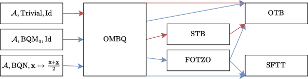
Figure 1: Summary of applications

Figure 1 captures the applications that are mentioned in Tables 1, 2 and 3. The exact statements are stated in Corollaries 6, 7 and 6 in the Appendix. To obtain a result from the graph, let ${\mathcal{A}}$ be one of SO-OGA or IA and select a directed path that has the following properties.

• The path starts at one of the three nodes on the left.

• The path must be at least of length 1 and the edges must be the same color.

• If ${\mathcal{A}}$ is IA, the path should not contain $\operatorname{SFTT}$ or $\operatorname{OTB}$.

For example, if ${\mathcal{A}}=\text{SO-OGA}$ and the path starts at the middle node on the left, then passes through $\operatorname{OMBQ}$, $\operatorname{FOTZO}$, $\operatorname{SFTT}$, we get

$$\operatorname{SFTT}(\operatorname{FOTZO}(\operatorname{OMBQ}(\text{SO-OGA},\operatorname{BQM0},\operatorname{Id})))$$

which is a projection-free algorithm (using separation oracles) with bandit feedback for monotone up-concave functions over convex sets that contain the origin. As mentioned in Table 3 and Corollary 6-(c), the adaptive regret of this algorithm is of order $O(T^{4/5})$. Note that the text written in the three nodes on the left correspond to the inputs of the meta-algorithm $\operatorname{OMBQ}$. Also note that the color red corresponds to the setting where ${\mathcal{G}}$ is a trivial query algorithm which means that the output of $\operatorname{OMBQ}$ is semi-bandit.

7 Conclusions

In this work, we have presented a comprehensive framework for addressing optimization problems involving upper quadratizable functions, encompassing both concave and DR-submodular functions across various settings and feedback types. Our contributions include the formulation of upper quadratizable functions as a generalized class, the development of meta-algorithms for algorithmic conversions, and the derivation of new projection-free algorithms with improved regret guarantees. By extending existing techniques from linear/quadratic optimization to upper quadratizable functions, we have significantly advanced the state-of-the-art in non-convex optimization.

Moreover, our results offer insights into the fundamental properties of optimization problems, shedding light on the connections between different function classes and algorithmic approaches. The versatility of our framework allows for seamless transitions between different feedback settings, enabling practitioners to tailor algorithms to specific application requirements. Furthermore, our results in dynamic and adaptive regret guarantees for DR-submodular maximization represent significant milestones in the field, opening up new avenues for research and application.

Appendix A Related works

DR-submodular maximization

Two of the main methods for continuous DR-submodular maximization are Frank-Wolfe type methods and Boosting based methods. This division is based on how the approximation coefficient appears in the proof.

In Frank-Wolfe type algorithms, the approximation coefficient appears by specific choices of the Frank-Wolfe update rules. (See Lemma 8 in [34]) The specific choices of the update rules for different settings have been proposed in [3, 2, 31, 36, 9]. The momentum technique of [30] has been used to convert algorithms designed for deterministic feedback to stochastic feedback setting. [18] proposed a Frank-Wolfe variant with access to a stochastic gradient oracle with known distribution. Frank-Wolfe type algorithms been adapted to the online setting using Meta-Frank-Wolfe [7, 8] or using Blackwell approachablity [32]. Later [44] used a Meta-Frank-Wolfe with random permutation technique to obtain full-information results that only require a single query per function and also bandit results. This was extended to another settings by [46] and generalized to many different settings with improved regret bounds by [34].

Another approach, referred to as boosting, is to construct an alternative function such that maximization of this function results in approximate maximization of the original function. Given this definition, we may consider the result of [19, 7, 12] as the first boosting based results. However, in these cases (i.e., the case of monotone DR-submodular functions over general convex sets), the alternative function is identical to the original function. The term boosting in this context was first used in [45] for monotone functions over convex sets containing the origin, based on ideas presented in [13, 29]. This idea was used later in [38, 26] in bandit and projection-free full-information settings. Finally, in [47] a boosting based method was introduced for non-monotone functions over general convex sets.

Up-concave maximization

Not all continuous DR-submodular functions are concave and not all concave functions are continuous DR-submodular. [29] considers functions that are the sum of a concave and a continuous DR-submodular function. It is well-known that continuous DR-submodular functions are concave along positive directions [5, 3]. Based on this idea, [40] defined an up-concave function as a function that is concave along positive directions. Up-concave maximization has been considered in the offline setting before, e.g. [24], but not in online setting. In this work, we focus on up-concave maximization which is a generalization of DR-submodular maximization.

Projection-free optimization

In the past decade, numerous projection-free online convex optimization algorithms have emerged to tackle the computational limitations of their projection-based counterparts [20, 6, 41, 8, 21, 15, 28, 16]. In the context of DR-submodular maximization, the Frank-Wolfe type methods discussed above are projection-free.

Non-stationary regret

Dynamic regret was first analyzed in [50] for first order deterministic feedback. Later [42] obtained the lower bound and optimal algorithm in this setting. This was later expanded to bandit setting in [48]. Adaptive regret was first analyzed in [22] and the first optimal algorithm for projection-free adaptive regret was proposed in [16]. We refer to  [22, 1, 10, 43, 42, 49, 48, 27, 39, 16] and references therein for more details.

Optimization by quadratization

The framework discussed here for analyzing online algorithms is based on the convex optimization framework introduced in [33]. We extend the framework to allows us to work with $\alpha$-regret.Moreover, [33] also demonstrates that algorithms that are designed for quadratic/linear optimization with fully adaptive adversary obtain a similar regret in the convex setting. In this paper we introduce the notion of quadratizable functions generalizes this idea beyond convex functions to all quadratizable functions. (see Theorem 1) This allows us to integrate the boosting method with our framework to obtain various meta-algorithms for continuous DR-submodular maximization.

Appendix B Problem Setup in Detail

In this section, we further expand on the description in Section 2.

A function class is a set of real-valued functions. Given a set ${\mathcal{D}}$, a function class over ${\mathcal{D}}$ is a subset of all real-valued functions on ${\mathcal{D}}$. A set ${\mathcal{K}}\subseteq{\mathbb{R}}^{d}$ is called a convex set if for all ${\mathbf{x}},{\mathbf{y}}\in{\mathcal{K}}$ and $\alpha\in[0,1]$, we have $\alpha{\mathbf{x}}+(1-\alpha){\mathbf{y}}\in{\mathcal{K}}$. For any ${\mathbf{u}}\in{\mathcal{K}}^{T}$, we define the path length $P_{T}({\mathbf{u}})\mathrel{\mathop{\mathchar 58\relax}}=\sum_{i=1}^{T-1}\|{\mathbf{u}}_{i}-{\mathbf{u}}_{i+1}\|.$

A real-valued differentiable function $f$ is called concave if $f(y)-f(x)\leq f^{\prime}(x)(y-x)$, for all $x,y\in\operatorname{Dom}(f)$. More generally, given $\mu\geq 0$ and $0<\gamma\leq 1$, we say a real-valued differentiable function is $\mu$-strongly $\gamma$-weakly concave if

$$f(y)-f(x)\leq\frac{1}{\gamma}\left(f(x)^{\prime}(y-x)-\frac{\mu}{2}|y-x|^{2}\right)$$

for all $x,y\in\operatorname{Dom}(f)$.

We say a differentiable function $f\mathrel{\mathop{\mathchar 58\relax}}{\mathcal{K}}\to{\mathbb{R}}$ is $\mu$-strongly $\gamma$-weakly up-concave if it is $\mu$-strongly $\gamma$-weakly concave along positive directions. Specifically if, for all ${\mathbf{x}}\leq{\mathbf{y}}$ in ${\mathcal{K}}$, we have

$$\gamma\left(\langle\nabla f({\mathbf{y}}),{\mathbf{y}}-{\mathbf{x}}\rangle+\frac{\mu}{2}\|{\mathbf{y}}-{\mathbf{x}}\|^{2}\right)\leq f({\mathbf{y}})-f({\mathbf{x}})\leq\frac{1}{\gamma}\left(\langle\nabla f({\mathbf{x}}),{\mathbf{y}}-{\mathbf{x}}\rangle-\frac{\mu}{2}\|{\mathbf{y}}-{\mathbf{x}}\|^{2}\right).$$

This notion could be generalized in the following manner. We say $\tilde{\nabla}f\mathrel{\mathop{\mathchar 58\relax}}{\mathcal{K}}\to{\mathbb{R}}^{d}$ is a $\mu$-strongly $\gamma$-weakly up-super-gradient of $f$ if for all ${\mathbf{x}}\leq{\mathbf{y}}$ in ${\mathcal{K}}$, we have

$$\gamma\left(\langle\tilde{\nabla}f({\mathbf{y}}),{\mathbf{y}}-{\mathbf{x}}\rangle+\frac{\mu}{2}\|{\mathbf{y}}-{\mathbf{x}}\|^{2}\right)\leq f({\mathbf{y}})-f({\mathbf{x}})\leq\frac{1}{\gamma}\left(\langle\tilde{\nabla}f({\mathbf{x}}),{\mathbf{y}}-{\mathbf{x}}\rangle-\frac{\mu}{2}\|{\mathbf{y}}-{\mathbf{x}}\|^{2}\right).$$

Then we say $f$ is $\mu$-strongly $\gamma$-weakly up-concave if it is continuous and it has a $\mu$-strongly $\gamma$-weakly up-super-gradient. When it is clear from the context, we simply refer to $\tilde{\nabla}f$ as an up-super-gradient for $f$. When $\gamma=1$ and the above inequality holds for all ${\mathbf{x}},{\mathbf{y}}\in{\mathcal{K}}$, we say $f$ is $\mu$-strongly concave.

A differentiable function $f\mathrel{\mathop{\mathchar 58\relax}}{\mathcal{K}}\to{\mathbb{R}}$ is called continuous DR-submodular if for all ${\mathbf{x}}\leq{\mathbf{y}}$, we have $\nabla f({\mathbf{x}})\geq\nabla f({\mathbf{y}})$. More generally, we say $f$ is $\gamma$-weakly continuous DR-submodular if for all ${\mathbf{x}}\leq{\mathbf{y}}$, we have $\nabla f({\mathbf{x}})\geq\gamma\nabla f({\mathbf{y}})$. It follows that any $\gamma$-weakly continuous DR-submodular functions is $\gamma$-weakly up-concave.

Given a continuous monotone function $f\mathrel{\mathop{\mathchar 58\relax}}{\mathcal{K}}\to{\mathbb{R}}$, its curvature is defined as the smallest number $c\in[0,1]$ such that

$$f({\mathbf{y}}+{\mathbf{z}})-f({\mathbf{y}})\geq(1-c)(f({\mathbf{x}}+{\mathbf{z}})-f({\mathbf{x}})),$$

for all ${\mathbf{x}},{\mathbf{y}}\in{\mathcal{K}}$ and ${\mathbf{z}}\geq 0$ such that ${\mathbf{x}}+{\mathbf{z}},{\mathbf{y}}+{\mathbf{z}}\in{\mathcal{K}}$. We define the curvature of a function class ${\mathbf{F}}$ as the supremum of the curvature of functions in ${\mathbf{F}}$.

Online optimization problems can be formalized as a repeated game between an agent and an adversary. The game lasts for $T$ rounds on a convex domain ${\mathcal{K}}$ where $T$ and ${\mathcal{K}}$ are known to both players. In $t$-th round, the agent chooses an action ${\mathbf{x}}_{t}$ from an action set ${\mathcal{K}}\subseteq{\mathbb{R}}^{d}$, then the adversary chooses a loss function $f_{t}\in{\mathbf{F}}$ and a query oracle for the function $f_{t}$. Then, for $1\leq i\leq k_{t}$, the agent chooses a points ${\mathbf{y}}_{t,i}$ and receives the output of the query oracle.

To be more precise, an agent consists of a tuple $(\Omega^{\mathcal{A}},{\mathcal{A}}^{\text{action}},{\mathcal{A}}^{\text{query}})$, where $\Omega^{\mathcal{A}}$ is a probability space that captures all the randomness of ${\mathcal{A}}$. We assume that, before the first action, the agent samples $\omega\in\Omega$. The next element in the tuple, ${\mathcal{A}}^{\text{action}}=({\mathcal{A}}^{\text{action}}_{1},\cdots,{\mathcal{A}}^{\text{action}}_{T})$ is a sequence of functions such that ${\mathcal{A}}_{t}$ that maps the history $\Omega^{\mathcal{A}}\times{\mathcal{K}}^{t-1}\times\prod_{s=1}^{t-1}({\mathcal{K}}\times{\mathcal{O}})^{k_{s}}$ to ${\mathbf{x}}_{t}\in{\mathcal{K}}$ where we use ${\mathcal{O}}$ to denote range of the query oracle. The last element in the tuple, ${\mathcal{A}}^{\text{query}}$, is the query policy. For each $1\leq t\leq T$ and $1\leq i\leq k_{t}$, ${\mathcal{A}}^{\text{query}}_{t,i}\mathrel{\mathop{\mathchar 58\relax}}\Omega^{\mathcal{A}}\times{\mathcal{K}}^{t}\times\prod_{s=1}^{t-1}({\mathcal{K}}\times{\mathcal{O}})^{k_{s}}\times({\mathcal{K}}\times{\mathcal{O}})^{i-1}$ is a function that, given previous actions and observations, either selects a point ${\mathbf{y}}_{t}^{i}\in{\mathcal{K}}$, i.e., query, or signals that the query policy at this time-step is terminated. We may drop $\omega$ as one of the inputs of the above functions when there is no ambiguity. We say the agent query function is trivial if $k_{t}=1$ and ${\mathbf{y}}_{t,1}={\mathbf{x}}_{t}$ for all $1\leq t\leq T$. In this case, we simplify the notation and use the notation ${\mathcal{A}}={\mathcal{A}}^{\text{action}}=({\mathcal{A}}_{1},\cdots,{\mathcal{A}}_{T})$ to denote the agent action functions and assume that the domain of ${\mathcal{A}}_{t}$ is $\Omega^{\mathcal{A}}\times({\mathcal{K}}\times{\mathcal{O}})^{t-1}$.

A query oracle is a function that provides the observation to the agent. Formally, a query oracle for a function $f$ is a map ${\mathcal{Q}}$ defined on ${\mathcal{K}}$ such that for each ${\mathbf{x}}\in{\mathcal{K}}$, the ${\mathcal{Q}}({\mathbf{x}})$ is a random variable taking value in the observation space ${\mathcal{O}}$. The query oracle is called a stochastic value oracle or stochastic zeroth order oracle if ${\mathcal{O}}={\mathbb{R}}$ and $f({\mathbf{x}})={\mathbb{E}}[{\mathcal{Q}}({\mathbf{x}})]$. Similarly, it is called a stochastic up-super-gradient oracle or stochastic first order oracle if ${\mathcal{O}}={\mathbb{R}}^{d}$ and ${\mathbb{E}}[{\mathcal{Q}}({\mathbf{x}})]$ is a up-super-gradient of $f$ at ${\mathbf{x}}$. In all cases, if the random variable takes a single value with probability one, we refer to it as a deterministic oracle. Note that, given a function, there is at most a single deterministic gradient oracle, but there may be many deterministic up-super-gradient oracles. We will use $\nabla$ to denote the deterministic gradient oracle. We say an oracle is bounded by $B$ if its output is always within the Euclidean ball of radius $B$ centered at the origin. We say the agent takes semi-bandit feedback if the oracle is first-order and the agent query function is trivial. Similarly, it takes bandit feedback if the oracle is zeroth-order and the agent query function is trivial. If the agent query function is non-trivial, then we say the agent requires full-information feedback.

An adversary $\operatorname{Adv}$ is a set such that each element ${\mathcal{B}}\in\operatorname{Adv}$, referred to as a realized adversary, is a sequence $({\mathcal{B}}_{1},\cdots,{\mathcal{B}}_{T})$ of functions where each ${\mathcal{B}}_{t}$ maps a tuple $({\mathbf{x}}_{1},\cdots,{\mathbf{x}}_{t})\in{\mathcal{K}}^{t}$ to a tuple $(f_{t},{\mathcal{Q}}_{t})$ where $f_{t}\in{\mathbf{F}}$ and ${\mathcal{Q}}_{t}$ is a query oracle for $f_{t}$. We say an adversary $\operatorname{Adv}$ is oblivious if for any realization ${\mathcal{B}}=({\mathcal{B}}_{1},\cdots,{\mathcal{B}}_{T})$, all functions ${\mathcal{B}}_{t}$ are constant, i.e., they are independent of $({\mathbf{x}}_{1},\cdots,{\mathbf{x}}_{t})$. In this case, a realized adversary may be simply represented by a sequence of functions $(f_{1},\cdots,f_{T})\in{\mathbf{F}}^{T}$ and a sequence of query oracles $({\mathcal{Q}}_{1},\cdots,{\mathcal{Q}}_{T})$ for these functions. We say an adversary is a weakly adaptive adversary if each function ${\mathcal{B}}_{t}$ described above does not depend on ${\mathbf{x}}_{t}$ and therefore may be represented as a map defined on ${\mathcal{K}}^{t-1}$. In this work we also consider adversaries that are fully adaptive, i.e., adversaries with no restriction. Clearly any oblivious adversary is a weakly adaptive adversary and any weakly adaptive adversary is a fully adaptive adversary. Given a function class ${\mathbf{F}}$ and $i\in\{0,1\}$, we use $\operatorname{Adv}^{\text{f}}_{i}({\mathbf{F}})$ to denote the set of all possible realized adversaries with deterministic $i$-th order oracles. If the oracle is instead stochastic and bounded by $B$, we use $\operatorname{Adv}^{\text{f}}_{i}({\mathbf{F}},B)$ to denote such an adversary. Finally, we use $\operatorname{Adv}^{\text{o}}_{i}({\mathbf{F}})$ and $\operatorname{Adv}^{\text{o}}_{i}({\mathbf{F}},B)$ to denote all oblivious realized adversaries with $i$-th order deterministic and stochastic oracles, respectively.

In order to handle different notions of regret with the same approach, for an agent ${\mathcal{A}}$, adversary $\operatorname{Adv}$, compact set ${\mathcal{U}}\subseteq{\mathcal{K}}^{T}$, approximation coefficient $0<\alpha\leq 1$ and $1\leq a\leq b\leq T$, we define regret as

$${\mathcal{R}}_{\alpha,\operatorname{Adv}}^{{\mathcal{A}}}({\mathcal{U}})[a,b]\mathrel{\mathop{\mathchar 58\relax}}=\sup_{{\mathcal{B}}\in\operatorname{Adv}}{\mathbb{E}}\left[\alpha\max_{{\mathbf{u}}=({\mathbf{u}}_{1},\cdots,{\mathbf{u}}_{T})\in{\mathcal{U}}}\sum_{t=a}^{b}f_{t}({\mathbf{u}}_{t})-\sum_{t=a}^{b}f_{t}({\mathbf{x}}_{t})\right],$$

where the expectation in the definition of the regret is over the randomness of the algorithm and the query oracle. We use the notation ${\mathcal{R}}_{\alpha,{\mathcal{B}}}^{{\mathcal{A}}}({\mathcal{U}})[a,b]\mathrel{\mathop{\mathchar 58\relax}}={\mathcal{R}}_{\alpha,\operatorname{Adv}}^{{\mathcal{A}}}({\mathcal{U}})[a,b]$ when $\operatorname{Adv}=\{{\mathcal{B}}\}$ is a singleton. We may drop $\alpha$ when it is equal to 1. When $\alpha<1$, we often assume that the functions are non-negative.

Static adversarial regret or simply adversarial regret corresponds to $a=1$, $b=T$ and ${\mathcal{U}}={\mathcal{K}}_{\star}^{T}\mathrel{\mathop{\mathchar 58\relax}}=\{({\mathbf{x}},\cdots,{\mathbf{x}})\mid{\mathbf{x}}\in{\mathcal{K}}\}$. When $a=1$, $b=T$ and ${\mathcal{U}}$ contains only a single element then it is referred to as the dynamic regret [50, 42]. Adaptive regret, is defined as $\max_{1\leq a\leq b\leq T}{\mathcal{R}}_{\alpha,\operatorname{Adv}}^{{\mathcal{A}}}({\mathcal{K}}_{\star}^{T})[a,b]$ [22]. We drop $a$, $b$ and ${\mathcal{U}}$ when the statement is independent of their value or their value is clear from the context.

Appendix C Proof of Theorem 1

The proof is similar to the proof of Theorems 2 and 5 in [33].

Proof.

Deterministic oracle:

We first consider the case where ${\mathcal{G}}$ is a deterministic query oracle for ${\mathfrak{g}}$. Let ${\mathbf{o}}_{t}={\mathfrak{g}}(f_{t},{\mathbf{x}}_{t})$ denote the output of ${\mathcal{G}}$ at time-step $t$. For any realization ${\mathcal{B}}=({\mathcal{B}}_{1},\cdots,{\mathcal{B}}_{T})\in\operatorname{Adv}_{1}^{\text{f}}({\mathbf{F}})$, we define ${\mathcal{B}}^{\prime}_{t}({\mathbf{x}}_{1},\cdots,{\mathbf{x}}_{t})$ to be the tuple $(q_{t},\nabla)$ where

$${\mathcal{B}}^{\prime}_{t}({\mathbf{x}}_{1},\cdots,{\mathbf{x}}_{t})\mathrel{\mathop{\mathchar 58\relax}}=q_{t}\mathrel{\mathop{\mathchar 58\relax}}={\mathbf{y}}\mapsto\langle{\mathbf{o}}_{t},{\mathbf{y}}-{\mathbf{x}}_{t}\rangle-\frac{\mu}{2}\|{\mathbf{y}}-{\mathbf{x}}_{t}\|^{2},$$

and ${\mathcal{B}}^{\prime}=({\mathcal{B}}^{\prime}_{1},\cdots,{\mathcal{B}}^{\prime}_{T})$. Note that each ${\mathcal{B}}^{\prime}_{t}$ is a deterministic function of ${\mathbf{x}}_{1},\cdots,{\mathbf{x}}_{t}$ and therefore ${\mathcal{B}}^{\prime}\in\operatorname{Adv}_{1}^{\text{f}}({\mathbf{F}}_{\mu,{\mathfrak{g}}})$. Since the algorithm uses semi-bandit feedback, the sequence of random vectors $({\mathbf{x}}_{1},\cdots,{\mathbf{x}}_{T})$ chosen by ${\mathcal{A}}$ is identical between the game with ${\mathcal{B}}$ and ${\mathcal{B}}^{\prime}$. Therefore, according to definition of quadratizable functions, for any ${\mathbf{y}}\in{\mathcal{K}}$, we have

$$\beta\left(q_{t}({\mathbf{y}})-q_{t}({\mathbf{x}}_{t})\right)=\beta\left(\langle{\mathbf{o}}_{t},{\mathbf{y}}-{\mathbf{x}}_{t}\rangle-\frac{\mu}{2}\|{\mathbf{y}}-{\mathbf{x}}_{t}\|^{2}\right)\geq\alpha f_{t}({\mathbf{y}})-f_{t}(h({\mathbf{x}}_{t})),$$

Therefore, we have

$$\max_{{\mathbf{u}}\in{\mathcal{U}}}\left(\alpha\sum_{t=a}^{b}f_{t}({\mathbf{u}}_{t})-\sum_{t=a}^{b}f_{t}(h({\mathbf{x}}_{t}))\right)\leq\beta\max_{{\mathbf{u}}\in{\mathcal{U}}}\left(\sum_{t=a}^{b}q_{t}({\mathbf{u}}_{t})-\sum_{t=a}^{b}q_{t}({\mathbf{x}}_{t})\right),$$ (4)

Hence

$${\mathcal{R}}_{\alpha,\operatorname{Adv}_{1}^{\text{f}}({\mathbf{F}})}^{{\mathcal{A}}^{\prime}} =\sup_{{\mathcal{B}}\in\operatorname{Adv}_{1}^{\text{f}}({\mathbf{F}})}{\mathcal{R}}_{\alpha,{\mathcal{B}}}^{{\mathcal{A}}^{\prime}}$$

$$=\sup_{{\mathcal{B}}\in\operatorname{Adv}_{1}^{\text{f}}({\mathbf{F}})}{\mathbb{E}}\left[\max_{{\mathbf{u}}\in{\mathcal{U}}}\left(\alpha\sum_{t=a}^{b}f_{t}({\mathbf{u}}_{t})-\sum_{t=a}^{b}f_{t}(h({\mathbf{x}}_{t}))\right)\right]$$

$$\leq\sup_{{\mathcal{B}}\in\operatorname{Adv}_{1}^{\text{f}}({\mathbf{F}})}{\mathbb{E}}\left[\beta\max_{{\mathbf{u}}\in{\mathcal{U}}}\left(\sum_{t=a}^{b}q_{t}({\mathbf{u}}_{t})-\sum_{t=a}^{b}q_{t}({\mathbf{x}}_{t})\right)\right]$$

$$\leq\beta\sup_{{\mathcal{B}}^{\prime}\in\operatorname{Adv}_{1}^{\text{f}}({\mathbf{F}}_{\mu,{\mathfrak{g}}})}{\mathcal{R}}_{1,{\mathcal{B}}^{\prime}}^{{\mathcal{A}}}=\beta{\mathcal{R}}_{1,\operatorname{Adv}_{1}^{\text{f}}({\mathbf{F}}_{\mu,{\mathfrak{g}}})}^{{\mathcal{A}}}.$$

Stochastic oracle:

Next we consider the case where ${\mathcal{G}}$ is a stochastic query oracle for ${\mathfrak{g}}$.

Let $\Omega^{\mathcal{Q}}=\Omega^{\mathcal{Q}}_{1}\times\cdots\times\Omega^{\mathcal{Q}}_{T}$ capture all sources of randomness in the query oracles of $\operatorname{Adv}_{1}^{\text{o}}({\mathbf{F}},B_{1})$, i.e., for any choice of $\theta\in\Omega^{\mathcal{Q}}$, the query oracle is deterministic. Hence for any $\theta\in\Omega^{\mathcal{Q}}$ and realized adversary ${\mathcal{B}}\in\operatorname{Adv}_{1}^{\text{o}}({\mathbf{F}},B_{1})$, we may consider ${\mathcal{B}}_{\theta}$ as an object similar to an adversary with a deterministic oracle. However, note that ${\mathcal{B}}_{\theta}$ does not satisfy the unbiasedness condition of the oracle, i.e., the returned value of the oracle is not necessarily the gradient of the function at that point. Recall that ${\mathcal{B}}_{t}$ maps a tuple $({\mathbf{x}}_{1},\cdots,{\mathbf{x}}_{t})$ to a tuple of $f_{t}$ and a stochastic query oracle for $f_{t}$. We will use ${\mathbb{E}}_{\Omega^{\mathcal{Q}}}$ to denote the expectation with respect to the randomness of query oracle and ${\mathbb{E}}_{\Omega^{\mathcal{Q}}_{t}}[\cdot]\mathrel{\mathop{\mathchar 58\relax}}={\mathbb{E}}_{\Omega^{\mathcal{Q}}}[\cdot|f_{t},{\mathbf{x}}_{t}]$ to denote the expectation conditioned on the history and the action of the agent. Similarly, let ${\mathbb{E}}_{\Omega^{\mathcal{A}}}$ denote the expectation with respect to the randomness of the agent. Let ${\mathbf{o}}_{t}$ be the random variable denoting the output of ${\mathcal{G}}$ at time-step $t$ and let

$$\bar{{\mathbf{o}}}_{t}\mathrel{\mathop{\mathchar 58\relax}}={\mathbb{E}}[{\mathbf{o}}_{t}\mid f_{t},{\mathbf{x}}_{t}]={\mathbb{E}}_{\Omega^{\mathcal{Q}}_{t}}[{\mathbf{o}}_{t}]={\mathfrak{g}}(f_{t},{\mathbf{x}}_{t}).$$

Similar to the deterministic case, for any realization ${\mathcal{B}}=(f_{1},\cdots,f_{T})\in\operatorname{Adv}^{\text{o}}({\mathbf{F}})$ and any $\theta\in\Omega^{\mathcal{Q}}$, we define ${\mathcal{B}}^{\prime}_{\theta,t}({\mathbf{x}}_{1},\cdots,{\mathbf{x}}_{t})$ to be the pair $(q_{t},\nabla)$ where

$$q_{t}\mathrel{\mathop{\mathchar 58\relax}}={\mathbf{y}}\mapsto\langle{\mathbf{o}}_{t},{\mathbf{y}}-{\mathbf{x}}_{t}\rangle-\frac{\mu}{2}\|{\mathbf{y}}-{\mathbf{x}}_{t}\|^{2}.$$

We also define ${\mathcal{B}}^{\prime}_{\theta}\mathrel{\mathop{\mathchar 58\relax}}=({\mathcal{B}}^{\prime}_{\theta,1},\cdots,{\mathcal{B}}^{\prime}_{\theta,T})$. Note that a specific choice of $\theta$ is necessary to make sure that the function returned by ${\mathcal{B}}^{\prime}_{\theta,t}$ is a deterministic function of ${\mathbf{x}}_{1},\cdots,{\mathbf{x}}_{t}$ and not a random variable and therefore ${\mathcal{B}}^{\prime}_{\theta}$ belongs to $\operatorname{Adv}_{1}^{\text{f}}({\mathbf{F}}_{\mu}[B_{1}])$.

Since the algorithm uses (semi-)bandit feedback, given a specific value of $\theta$, the sequence of random vectors $({\mathbf{x}}_{1},\cdots,{\mathbf{x}}_{T})$ chosen by ${\mathcal{A}}$ is identical between the game with ${\mathcal{B}}_{\theta}$ and ${\mathcal{B}}^{\prime}_{\theta}$. Therefore, for any ${\mathbf{u}}_{t}\in{\mathcal{K}}$, we have

$$\alpha f_{t}({\mathbf{u}}_{t})-f_{t}(h({\mathbf{x}}_{t})) \leq\beta\left(\langle\bar{{\mathbf{o}}}_{t},{\mathbf{u}}_{t}-{\mathbf{x}}_{t}\rangle-\frac{\mu}{2}\|{\mathbf{u}}_{t}-{\mathbf{x}}_{t}\|^{2}\right)$$

$$=\beta\left(\langle{\mathbb{E}}\left[{\mathbf{o}}_{t}\mid f_{t},{\mathbf{x}}_{t}\right],{\mathbf{u}}_{t}-{\mathbf{x}}_{t}\rangle-\frac{\mu}{2}\|{\mathbf{u}}_{t}-{\mathbf{x}}_{t}\|^{2}\right)$$

$$=\beta\left({\mathbb{E}}\left[\langle{\mathbf{o}}_{t},{\mathbf{u}}_{t}-{\mathbf{x}}_{t}\rangle-\frac{\mu}{2}\|{\mathbf{u}}_{t}-{\mathbf{x}}_{t}\|^{2}\mid f_{t},{\mathbf{x}}_{t}\right]\right)$$

$$=\beta\left({\mathbb{E}}\left[q_{t}({\mathbf{u}}_{t})-q_{t}({\mathbf{x}}_{t})\mid f_{t},{\mathbf{x}}_{t}\right]\right),$$

where the first inequality follows from the fact that $f_{t}$ is up-quadratizable and $\bar{{\mathbf{o}}}_{t}={\mathfrak{g}}(f_{t},{\mathbf{x}}_{t})$. Therefore we have

$${\mathbb{E}}\left[\alpha\sum_{t=a}^{b}f_{t}({\mathbf{u}}_{t})-\sum_{t=a}^{b}f_{t}(h({\mathbf{x}}_{t}))\right] \leq\beta{\mathbb{E}}\left[\sum_{t=a}^{b}{\mathbb{E}}\left[q_{t}({\mathbf{u}}_{t})-q_{t}({\mathbf{x}}_{t})|f_{t},{\mathbf{x}}_{t}\right]\right]$$

$$=\beta{\mathbb{E}}\left[\sum_{t=a}^{b}q_{t}({\mathbf{u}}_{t})-q_{t}({\mathbf{x}}_{t})\right].$$

Since ${\mathcal{B}}$ is oblivious, the sequence $(f_{1},\cdots,f_{T})$ is not affected by the randomness of query oracles or the agent. Therefore we have

$${\mathcal{R}}_{\alpha,{\mathcal{B}}}^{{\mathcal{A}}} ={\mathbb{E}}\left[\alpha\max_{{\mathbf{u}}\in{\mathcal{U}}}\sum_{t=a}^{b}f_{t}({\mathbf{u}}_{t})-\sum_{t=a}^{b}f_{t}(h({\mathbf{x}}_{t}))\right]$$

$$=\max_{{\mathbf{u}}\in{\mathcal{U}}}{\mathbb{E}}\left[\alpha\sum_{t=a}^{b}f_{t}({\mathbf{u}}_{t})-\sum_{t=a}^{b}f_{t}(h({\mathbf{x}}_{t}))\right]$$

$$\leq\beta\max_{{\mathbf{u}}\in{\mathcal{U}}}{\mathbb{E}}\left[\sum_{t=a}^{b}q_{t}({\mathbf{u}}_{t})-\sum_{t=a}^{b}q_{t}({\mathbf{x}}_{t})\right]$$

$$\leq\beta{\mathbb{E}}\left[\max_{{\mathbf{u}}\in{\mathcal{U}}}\left(\sum_{t=a}^{b}q_{t}({\mathbf{u}}_{t})-\sum_{t=a}^{b}q_{t}({\mathbf{x}}_{t})\right)\right]=\beta{\mathbb{E}}\left[{\mathcal{R}}_{1,{\mathcal{B}}^{\prime}_{\theta}}^{{\mathcal{A}}}\right],$$

where the second inequality follows from Jensen’s inequality. Hence we have

$${\mathcal{R}}_{\alpha,\operatorname{Adv}_{1}^{\text{o}}({\mathbf{F}},B_{1})}^{{\mathcal{A}}} =\sup_{{\mathcal{B}}\in\operatorname{Adv}_{1}^{\text{o}}({\mathbf{F}},B_{1})}{\mathcal{R}}_{\alpha,{\mathcal{B}}}^{{\mathcal{A}}}\leq\sup_{{\mathcal{B}}\in\operatorname{Adv}_{1}^{\text{o}}({\mathbf{F}},B_{1}),\theta\in\Omega^{\mathcal{Q}}}\beta{\mathcal{R}}_{1,{\mathcal{B}}^{\prime}_{\theta}}^{{\mathcal{A}}}$$

$$\leq\sup_{{\mathcal{B}}^{\prime}\in\operatorname{Adv}_{1}^{\text{f}}({\mathbf{F}}_{\mu}[B_{1}])}\beta{\mathcal{R}}_{1,{\mathcal{B}}^{\prime}}^{{\mathcal{A}}}=\beta{\mathcal{R}}_{\operatorname{Adv}_{1}^{\text{f}}(1,{\mathbf{F}}_{\mu}[B_{1}])}^{{\mathcal{A}}}\qed$$

Appendix D Proof of Lemma 1

Proof.

We have ${\mathbf{x}}\vee{\mathbf{y}}+{\mathbf{x}}\wedge{\mathbf{y}}={\mathbf{x}}+{\mathbf{y}}$. Therefore, following the definition of curvature, we have

$$f({\mathbf{x}}\vee{\mathbf{y}})-f({\mathbf{y}})\geq(1-c)(f({\mathbf{x}})-f({\mathbf{x}}\wedge{\mathbf{y}})).$$

Since $f$ is non-negative, this implies that

$$(f({\mathbf{x}}\vee{\mathbf{y}})-f({\mathbf{x}})) +\frac{1}{\gamma^{2}}(f({\mathbf{x}}\wedge{\mathbf{y}})-f({\mathbf{x}}))$$ (5)

$$=(f({\mathbf{y}})-f({\mathbf{x}}))+(f({\mathbf{x}}\vee{\mathbf{y}})-f({\mathbf{y}}))+\frac{1}{\gamma^{2}}(f({\mathbf{x}}\wedge{\mathbf{y}})-f({\mathbf{x}}))$$

$$\geq(f({\mathbf{y}})-f({\mathbf{x}}))+(1-c-\frac{1}{\gamma^{2}})(f({\mathbf{x}})-f({\mathbf{x}}\wedge{\mathbf{y}}))$$

$$=f({\mathbf{y}})-(c+\frac{1}{\gamma^{2}})f({\mathbf{x}})+(-1+c+\frac{1}{\gamma^{2}})f({\mathbf{x}}\wedge{\mathbf{y}})$$

$$\geq f({\mathbf{y}})-(c+\frac{1}{\gamma^{2}})f({\mathbf{x}}).$$

On the other hand, according to the definition, we have

$$f({\mathbf{x}}\vee{\mathbf{y}})-f({\mathbf{x}}) \leq\frac{1}{\gamma}\left(\langle\tilde{\nabla}f({\mathbf{x}}),{\mathbf{x}}\vee{\mathbf{y}}-{\mathbf{x}}\rangle-\frac{\mu}{2}\|{\mathbf{x}}\vee{\mathbf{y}}-{\mathbf{x}}\|^{2}\right),$$

$$f({\mathbf{x}})-f({\mathbf{x}}\wedge{\mathbf{y}}) \geq\gamma\left(\langle\tilde{\nabla}f({\mathbf{x}}),{\mathbf{x}}-{\mathbf{x}}\wedge{\mathbf{y}}\rangle+\frac{\mu}{2}\|{\mathbf{x}}-{\mathbf{x}}\wedge{\mathbf{y}}\|^{2}\right).$$

Therefore, using Inequality 5 and the fact that $f({\mathbf{x}}\wedge{\mathbf{y}})\geq 0$, we see that

$$f({\mathbf{y}})-\frac{1+c\gamma^{2}}{\gamma^{2}}f({\mathbf{x}}) \leq(f({\mathbf{x}}\vee{\mathbf{y}})-f({\mathbf{x}}))+\frac{1}{\gamma^{2}}(f({\mathbf{x}}\wedge{\mathbf{y}})-f({\mathbf{x}}))$$

$$\leq\frac{1}{\gamma}\left(\langle\tilde{\nabla}f({\mathbf{x}}),{\mathbf{x}}\vee{\mathbf{y}}-{\mathbf{x}}\rangle-\frac{\mu}{2}\|{\mathbf{x}}\vee{\mathbf{y}}-{\mathbf{x}}\|^{2}+\langle\tilde{\nabla}f({\mathbf{x}}),{\mathbf{x}}\wedge{\mathbf{y}}-{\mathbf{x}}\rangle\right.$$

$$\qquad\qquad\left.-\frac{\mu}{2}\|{\mathbf{x}}-{\mathbf{x}}\wedge{\mathbf{y}}\|^{2}\right)$$

$$=\frac{1}{\gamma}\left(\langle\tilde{\nabla}f({\mathbf{x}}),{\mathbf{x}}\vee{\mathbf{y}}+{\mathbf{x}}\wedge{\mathbf{y}}-2{\mathbf{x}}\rangle-\frac{\mu}{2}\|{\mathbf{x}}\vee{\mathbf{y}}-{\mathbf{x}}\|^{2}-\frac{\mu}{2}\|{\mathbf{x}}-{\mathbf{x}}\wedge{\mathbf{y}}\|^{2}\right)$$

$$=\frac{1}{\gamma}\left(\langle\tilde{\nabla}f({\mathbf{x}}),{\mathbf{y}}-{\mathbf{x}}\rangle-\frac{\mu}{2}\|{\mathbf{x}}-{\mathbf{y}}\|^{2}\right),$$

where we used ${\mathbf{x}}\vee{\mathbf{y}}+{\mathbf{x}}\wedge{\mathbf{y}}={\mathbf{x}}+{\mathbf{y}}$ and

$$\|{\mathbf{x}}\vee{\mathbf{y}}-{\mathbf{x}}\|^{2}+\|{\mathbf{x}}-{\mathbf{x}}\wedge{\mathbf{y}}\|^{2} =\sum_{[y]_{i}\geq[x]_{i}}(y_{i}-x_{i})^{2}+\sum_{[y]_{i}<[x]_{i}}(x_{i}-y_{i})^{2}$$

$$=\sum_{i}(x_{i}-y_{i})^{2}=\|{\mathbf{x}}-{\mathbf{y}}\|^{2}$$

in the last equality. The claim now follows from multiply both sides by $\frac{\gamma^{2}}{1+c\gamma^{2}}$. ∎

Appendix E Proof of Lemma 2

Proof.

Clearly we have $F({\mathbf{0}})=0$. For any ${\mathbf{x}}\neq{\mathbf{0}}$, the integrand in the definition of $F$ is a continuous non-negative function of $z$ that is bounded by

$$\frac{\gamma e^{\gamma(z-1)}}{(1-e^{-\gamma})z}(f(z*{\mathbf{x}})-f({\mathbf{0}}))\leq\frac{\gamma e^{\gamma(z-1)}}{(1-e^{-\gamma})z}M_{1}\|z*{\mathbf{x}}\|\leq\frac{\gamma}{1-e^{-\gamma}}M_{1}\|{\mathbf{x}}\|.$$

Therefore $F$ is well-defined on $[0,1]^{d}$. Moreover, we have

$$\int_{0}^{1}\frac{\gamma e^{\gamma(z-1)}}{(1-e^{-\gamma})}\nabla f(z*{\mathbf{x}})dz=\nabla\int_{0}^{1}\frac{\gamma e^{\gamma(z-1)}}{(1-e^{-\gamma})z}(f(z*{\mathbf{x}})-f({\mathbf{0}}))dz=\nabla F({\mathbf{x}}).$$

It follows that $F$ is differentiable everywhere and ${\mathbb{E}}\left[\nabla f({\mathcal{Z}}*{\mathbf{x}})\right]=\nabla F({\mathbf{x}})$. To prove the last claim, first we note that

$$\frac{1-e^{-\gamma}}{\gamma}\langle\nabla F({\mathbf{x}}),{\mathbf{x}}\rangle =\left\langle\int_{0}^{1}e^{\gamma(z-1)}\nabla f(z*{\mathbf{x}})dz,{\mathbf{x}}\right\rangle$$

$$=\int_{0}^{1}e^{\gamma(z-1)}\langle\nabla f(z*{\mathbf{x}}),{\mathbf{x}}\rangle dz$$

$$=\int_{0}^{1}e^{\gamma(z-1)}df(z*{\mathbf{x}})$$

$$=e^{\gamma(z-1)}f(z*{\mathbf{x}})|_{z=0}^{z=1}-\int_{0}^{1}f(z*{\mathbf{x}})\frac{de^{\gamma(z-1)}}{dz}dz$$

$$=f({\mathbf{x}})-f({\mathbf{0}})-\int_{0}^{1}\gamma e^{\gamma(z-1)}f(z*{\mathbf{x}})dz.$$

On the other hand, using monotonicity and up-concavity of $f$, we have

$$\frac{1-e^{-\gamma}}{\gamma}\langle\nabla F({\mathbf{x}}),{\mathbf{y}}\rangle =\int_{0}^{1}e^{\gamma(z-1)}\langle\nabla f(z*{\mathbf{x}}),{\mathbf{y}}\rangle dz$$

$$\geq\int_{0}^{1}e^{\gamma(z-1)}\langle\nabla f(z*{\mathbf{x}}),{\mathbf{y}}\vee(z*{\mathbf{x}})-z*{\mathbf{x}}\rangle dz$$

$$\geq\int_{0}^{1}\gamma e^{\gamma(z-1)}\left(f({\mathbf{y}}\vee(z*{\mathbf{x}}))-f(z*{\mathbf{x}})\right)dz$$

$$\geq\int_{0}^{1}\gamma e^{\gamma(z-1)}\left(f({\mathbf{y}})-f(z*{\mathbf{x}})\right)dz$$

$$=(1-e^{-\gamma})f({\mathbf{y}})-\left(\int_{0}^{1}\gamma e^{\gamma(z-1)}f(z*{\mathbf{x}})dz\right),$$

where we used $\int_{0}^{1}e^{\gamma(z-1)}\gamma dz=1-e^{-\gamma}$ in the last equality. Therefore

$$\frac{1-e^{-\gamma}}{\gamma}\langle\nabla F({\mathbf{x}}),{\mathbf{y}}-{\mathbf{x}}\rangle \geq(1-e^{-\gamma})f({\mathbf{y}})-f({\mathbf{x}})+f({\mathbf{0}})\geq(1-e^{-\gamma})f({\mathbf{y}})-f({\mathbf{x}}).\qed$$

Appendix F Proof of Lemma 3

We start by stating a useful lemma from the literature.

Lemma 4 (Lemma 2.2 of [31]).

For any two vectors ${\mathbf{x}},{\mathbf{y}}\in[0,1]^{d}$ and any continuously differentiable non-negative DR-submodular function $f$ we have

$$f({\mathbf{x}}\vee{\mathbf{y}})\geq(1-\|{\mathbf{x}}\|_{\infty})f({\mathbf{y}}).$$

Proof of Lemma 3.

Clearly we have $F(\underline{{\mathbf{x}}})=0$. For any ${\mathbf{x}}\neq\underline{{\mathbf{x}}}$, the integrand in the definition of $F$ is a continuous function of $z$ that is bounded by

$$\left|\frac{2}{3z(1-\frac{z}{2})^{3}}\left(f\left(\frac{z}{2}*({\mathbf{x}}-\underline{{\mathbf{x}}})+\underline{{\mathbf{x}}}\right)-f(\underline{{\mathbf{x}}})\right)\right| \leq\frac{2}{3z(1-\frac{z}{2})^{3}}M_{1}\|\frac{z}{2}*({\mathbf{x}}-\underline{{\mathbf{x}}})\|\leq\frac{8}{3}M_{1}\|{\mathbf{x}}-\underline{{\mathbf{x}}}\|.$$

Therefore $F$ is well-defined on $[0,1]^{d}$. Moreover, we have

$$\int_{0}^{1}\frac{1}{3(1-\frac{z}{2})^{3}}\nabla f\left(\frac{z}{2}*({\mathbf{x}}-\underline{{\mathbf{x}}})+\underline{{\mathbf{x}}}\right)dz =\nabla\int_{0}^{1}\frac{2}{3z(1-\frac{z}{2})^{3}}\left(f\left(\frac{z}{2}*({\mathbf{x}}-\underline{{\mathbf{x}}})+\underline{{\mathbf{x}}}\right)-f(\underline{{\mathbf{x}}})\right)dz$$

$$=\nabla F({\mathbf{x}})$$

It follows that $F$ is differentiable everywhere and ${\mathbb{E}}\left[\nabla f\left(\frac{{\mathcal{Z}}}{2}*({\mathbf{x}}-\underline{{\mathbf{x}}})+\underline{{\mathbf{x}}}\right)\right]=\nabla F({\mathbf{x}})$.

To prove the last claim, let ${\mathbf{x}}_{z}\mathrel{\mathop{\mathchar 58\relax}}=\frac{z}{2}*({\mathbf{x}}-\underline{{\mathbf{x}}})+\underline{{\mathbf{x}}}$ and $\omega(z)=\frac{1}{8(1-\frac{z}{2})^{3}}$. We have

$$\frac{3}{8}\langle\nabla F({\mathbf{x}}),{\mathbf{y}}\rangle =\int_{0}^{1}\omega(z)\langle\nabla f({\mathbf{x}}_{z}),{\mathbf{y}}\rangle dz$$

$$=\int_{0}^{1}\omega(z)\left(\langle\nabla f({\mathbf{x}}_{z}),{\mathbf{y}}-{\mathbf{x}}_{z}\wedge{\mathbf{y}}\rangle+\langle\nabla f({\mathbf{x}}_{z}),{\mathbf{x}}_{z}\wedge{\mathbf{y}}-{\mathbf{x}}_{z}\rangle+\langle\nabla f({\mathbf{x}}_{z}),{\mathbf{x}}_{z}\rangle\right)dz$$

$$=\int_{0}^{1}\omega(z)\left(\langle\nabla f({\mathbf{x}}_{z}),{\mathbf{x}}_{z}\vee{\mathbf{y}}-{\mathbf{x}}_{z}\rangle+\langle\nabla f({\mathbf{x}}_{z}),{\mathbf{x}}_{z}\wedge{\mathbf{y}}-{\mathbf{x}}_{z}\rangle+\langle\nabla f({\mathbf{x}}_{z}),{\mathbf{x}}_{z}\rangle\right)dz$$

$$\geq\int_{0}^{1}\omega(z)\left((f({\mathbf{x}}_{z}\vee{\mathbf{y}})-f({\mathbf{x}}_{z}))+(f({\mathbf{x}}_{z}\wedge{\mathbf{y}})-f({\mathbf{x}}_{z}))+\langle\nabla f({\mathbf{x}}_{z}),{\mathbf{x}}_{z}\rangle\right)dz$$

$$\geq\int_{0}^{1}\omega(z)\left(f({\mathbf{x}}_{z}\vee{\mathbf{y}})-2f({\mathbf{x}}_{z})+\langle\nabla f({\mathbf{x}}_{z}),{\mathbf{x}}_{z}\rangle\right)dz.$$

Using Lemma 4, we have

$$f({\mathbf{x}}_{z}\vee{\mathbf{y}}) \geq(1-\|{\mathbf{x}}_{z}\|_{\infty})f(y)$$

$$\geq\left(1-\left(\left(1-\frac{z}{2}\right)\|\underline{{\mathbf{x}}}\|_{\infty}+\frac{z}{2}\|{\mathbf{x}}\|_{\infty}\right)\right)f(y)$$

$$\geq\left(1-\left(\left(1-\frac{z}{2}\right)\|\underline{{\mathbf{x}}}\|_{\infty}+\frac{z}{2}\right)\right)f(y)$$

$$=\left(1-\frac{z}{2}\right)\left(1-\|\underline{{\mathbf{x}}}\|_{\infty}\right)f(y).$$

Therefore

$$\frac{3}{8}\langle\nabla F({\mathbf{x}}),{\mathbf{y}}\rangle \geq\int_{0}^{1}\omega(z)\left(\left(1-\frac{z}{2}\right)\left(1-\|\underline{{\mathbf{x}}}\|_{\infty}\right)f(y)-2f({\mathbf{x}}_{z})+\langle\nabla f({\mathbf{x}}_{z}),{\mathbf{x}}_{z}\rangle\right)dz.$$ (6)

Next we bound $\langle\nabla F({\mathbf{x}}),{\mathbf{x}}\rangle$. We have

$$\frac{3}{8}\langle\nabla F({\mathbf{x}}),{\mathbf{x}}\rangle=\int_{0}^{1}\omega(z)\langle\nabla f({\mathbf{x}}),{\mathbf{x}}-{\mathbf{x}}_{z}\rangle dz+\int_{0}^{1}\omega(z)\langle\nabla f({\mathbf{x}}),{\mathbf{x}}_{z}\rangle dz$$

For the first term, we have

$$\int_{0}^{1}\omega(z)\langle\nabla f({\mathbf{x}}),{\mathbf{x}}-{\mathbf{x}}_{z}\rangle dz =\int_{0}^{1}\omega(z)\left\langle\nabla f({\mathbf{x}}),\left(1-\frac{z}{2}\right)({\mathbf{x}}-\underline{{\mathbf{x}}})\right\rangle dz$$

$$=\int_{0}^{1}(2-z)\omega(z)\left\langle\nabla f({\mathbf{x}}),\frac{{\mathbf{x}}-\underline{{\mathbf{x}}}}{2}\right\rangle dz$$

$$=\int_{0}^{1}(2-z)\omega(z)df({\mathbf{x}}_{z})$$

$$=(2-z)\omega(z)f({\mathbf{x}}_{z})|_{z=0}^{1}-\int_{0}^{1}((2-z)\omega^{\prime}(z)-\omega(z))f({\mathbf{x}}_{z})dz$$

$$=f({\mathbf{x}}_{1})-\frac{1}{4}f(\underline{{\mathbf{x}}})-\int_{0}^{1}\frac{1}{4(1-\frac{z}{2})^{3}}f({\mathbf{x}}_{z})dz,$$

which implies that

$$\frac{3}{8}\langle\nabla F({\mathbf{x}}),{\mathbf{x}}\rangle =f({\mathbf{x}}_{1})-\frac{1}{4}f(\underline{{\mathbf{x}}})-\int_{0}^{1}\frac{1}{4(1-\frac{z}{2})^{3}}f({\mathbf{x}}_{z})dz+\int_{0}^{1}\omega(z)\langle\nabla f({\mathbf{x}}),{\mathbf{x}}_{z}\rangle dz$$

$$\leq f({\mathbf{x}}_{1})-\int_{0}^{1}2\omega(z)f({\mathbf{x}}_{z})dz+\int_{0}^{1}\omega(z)\langle\nabla f({\mathbf{x}}),{\mathbf{x}}_{z}\rangle dz$$ (7)

Combining Equations 6 and F, we have

$$\frac{3}{8}\langle\nabla F({\mathbf{x}}),{\mathbf{y}}-{\mathbf{x}}\rangle \geq\int_{0}^{1}\omega(z)\left(\left(1-\frac{z}{2}\right)\left(1-\|\underline{{\mathbf{x}}}\|_{\infty}\right)f(y)-2f({\mathbf{x}}_{z})+\langle\nabla f({\mathbf{x}}_{z}),{\mathbf{x}}_{z}\rangle\right)dz$$

$$\qquad-f({\mathbf{x}}_{1})+\int_{0}^{1}2\omega(z)f({\mathbf{x}}_{z})dz-\int_{0}^{1}\omega(z)\langle\nabla f({\mathbf{x}}),{\mathbf{x}}_{z}\rangle dz$$

$$=\frac{1-\|\underline{{\mathbf{x}}}\|_{\infty}}{4}f({\mathbf{y}})\int_{0}^{1}4\left(1-\frac{z}{2}\right)\omega(z)dz-f({\mathbf{x}}_{1})$$

$$=\frac{1-\|\underline{{\mathbf{x}}}\|_{\infty}}{4}f({\mathbf{y}})-f\left(\frac{{\mathbf{x}}+\underline{{\mathbf{x}}}}{2}\right).\qed$$

Appendix G Proof of Theorem 6

The algorithms are special cases of Algorithms 2 and 3 in [33] where the shrinking parameter and the smoothing parameter are equal. We include a description of the algorithms for completion.

Input :  Shrunk domain $\hat{{\mathcal{K}}}_{\alpha}$, Linear space ${\mathcal{L}}_{0}$, smoothing parameter $\delta\leq\alpha$, horizon $T$, algorithm ${\mathcal{A}}$

Pass $\hat{{\mathcal{K}}}_{\alpha}$ as the domain to ${\mathcal{A}}$

$k\leftarrow\operatorname{dim}({\mathcal{L}}_{0})$

for $t=1,2,\dots,T$ do

       ${\mathbf{x}}_{t}\leftarrow$ the action chosen by ${\mathcal{A}}$

       Play ${\mathbf{x}}_{t}$

       Let $f_{t}$ be the function chosen by the adversary

       for $i$ starting from 1, while ${\mathcal{A}}^{\text{query}}$ is not terminated for this time-step do

             Sample ${\mathbf{v}}_{t,i}\in{\mathbb{S}}^{1}\cap{\mathcal{L}}_{0}$ uniformly

             Let ${\mathbf{y}}_{t,i}$ be the query chosen by ${\mathcal{A}}^{\text{query}}$

             Query the oracle at the point ${\mathbf{y}}_{t,i}+\delta{\mathbf{v}}_{t,i}$ to get $o_{t,i}$

             Pass $\frac{k}{\delta}o_{t}{\mathbf{v}}_{t}$ as the oracle output to ${\mathcal{A}}$

            

       end for

      

end for

Algorithm 5 First order to zeroth order - $\operatorname{FOTZO}({\mathcal{A}})$

Input :  Shrunk domain $\hat{{\mathcal{K}}}_{\alpha}$, Linear space ${\mathcal{L}}_{0}$, smoothing parameter $\delta\leq\alpha$, horizon $T$, algorithm ${\mathcal{A}}$

Pass $\hat{{\mathcal{K}}}_{\alpha}$ as the domain to ${\mathcal{A}}$

$k\leftarrow\operatorname{dim}({\mathcal{L}}_{0})$

for $t=1,2,\dots,T$ do

       Sample ${\mathbf{v}}_{t}\in{\mathbb{S}}^{1}\cap{\mathcal{L}}_{0}$ uniformly

       ${\mathbf{x}}_{t}\leftarrow$ the action chosen by ${\mathcal{A}}$

       Play ${\mathbf{x}}_{t}+\delta{\mathbf{v}}_{t}$

       Let $f_{t}$ be the function chosen by the adversary

       Let $o_{t}$ be the output of the value oracle

       Pass $\frac{k}{\delta}o_{t}{\mathbf{v}}_{t}$ as the oracle output to ${\mathcal{A}}$

      

end for

Algorithm 6 Semi-bandit to bandit - $\operatorname{STB}({\mathcal{A}})$

The proof of Theorem 6 is similar to the proof of Theorems 6 and 7 in [33]. The only difference being that we prove the result for $\alpha$-regret instead of regret. We include a proof for completion.

Proof.

Regret bound for $\operatorname{STB}$:

Note that any realized adversary ${\mathcal{B}}\in\operatorname{Adv}^{\text{o}}_{0}({\mathbf{F}},B_{0})$ may be represented as a sequence of functions $(f_{1},\cdots,f_{T})$ and a corresponding sequence of query oracles $({\mathcal{Q}}_{1},\cdots,{\mathcal{Q}}_{T})$. For such realized adversary ${\mathcal{B}}$, we define $\hat{B}$ to be the realized adversary corresponding to $(\hat{f}_{1},\cdots,\hat{f}_{T})$ with the stochastic gradient oracles

$$\hat{{\mathcal{Q}}}_{t}({\mathbf{x}})\mathrel{\mathop{\mathchar 58\relax}}=\frac{k}{\delta}{\mathcal{Q}}_{t}({\mathbf{x}}+\delta{\mathbf{v}}){\mathbf{v}},$$ (8)

where ${\mathbf{v}}$ is a random vector, taking its values uniformly from ${\mathbb{S}}^{1}\cap{\mathcal{L}}_{0}={\mathbb{S}}^{1}\cap(\operatorname{aff}({\mathcal{K}})-{\mathbf{z}})$, for any ${\mathbf{z}}\in{\mathcal{K}}$ and $k=\operatorname{dim}({\mathcal{L}}_{0})$. Since ${\mathcal{Q}}_{t}$ is a stochastic value oracle for $f_{t}$, according to Remark 4 in [36], $\hat{{\mathcal{Q}}}_{t}({\mathbf{x}})$ is an unbiased estimator of $\nabla\hat{f}_{t}({\mathbf{x}})$. Hence we have $\hat{B}\in\operatorname{Adv}_{1}^{\text{o}}(\hat{{\mathbf{F}}},\frac{k}{\delta}B_{0})$. Using Equation 8 and the definition of the Algorithm 6, we see that the responses of the queries are the same between the game $({\mathcal{A}},\hat{{\mathcal{B}}})$ and $({\mathcal{A}}^{\prime},{\mathcal{B}})$. It follows that the sequence of actions $({\mathbf{x}}_{1},\cdots,{\mathbf{x}}_{T})$ in $({\mathcal{A}},\hat{{\mathcal{B}}})$ corresponds to the sequence of actions $({\mathbf{x}}_{1}+\delta{\mathbf{v}}_{1},\cdots,{\mathbf{x}}_{T}+\delta{\mathbf{v}}_{T})$ in $({\mathcal{A}}^{\prime},{\mathcal{B}})$.

Let ${\mathbf{u}}\in\operatorname{argmax}_{{\mathbf{u}}\in{\mathcal{U}}}\sum_{t=a}^{b}f_{t}({\mathbf{u}}_{t})$ and $\hat{{\mathbf{u}}}\in\operatorname{argmax}_{{\mathbf{u}}\in\hat{{\mathcal{U}}}}\sum_{t=a}^{b}\hat{f_{t}}({\mathbf{u}}_{t})$. We have

$${\mathcal{R}}_{\alpha,{\mathcal{B}}}^{{\mathcal{A}}^{\prime}}-{\mathcal{R}}_{\alpha,\hat{{\mathcal{B}}}}^{{\mathcal{A}}} ={\mathbb{E}}\left[\alpha\sum_{t=a}^{b}f_{t}({\mathbf{u}}_{t})-\sum_{t=a}^{b}f_{t}({\mathbf{x}}_{t}+\delta{\mathbf{v}}_{t})\right]-{\mathbb{E}}\left[\alpha\sum_{t=a}^{b}\hat{f_{t}}(\hat{{\mathbf{u}}}_{t})-\sum_{t=a}^{b}\hat{f_{t}}({\mathbf{x}}_{t})\right]$$

$$={\mathbb{E}}\left[\left(\sum_{t=a}^{b}\hat{f_{t}}({\mathbf{x}}_{t})-\sum_{t=a}^{b}f_{t}({\mathbf{x}}_{t}+\delta{\mathbf{v}}_{t})\right)+\alpha\left(\sum_{t=a}^{b}f_{t}({\mathbf{u}}_{t})-\sum_{t=a}^{b}\hat{f_{t}}(\hat{{\mathbf{u}}}_{t})\right)\right].$$ (9)

According to Lemma 3 in [36], we have $|\hat{f_{t}}({\mathbf{x}}_{t})-f_{t}({\mathbf{x}}_{t})|\leq\delta M_{1}$. By using Lipschitz property for the pair $({\mathbf{x}}_{t},{\mathbf{x}}_{t}+\delta{\mathbf{v}}_{t})$, we see that

$$|f_{t}({\mathbf{x}}_{t}+\delta{\mathbf{v}}_{t})-\hat{f_{t}}({\mathbf{x}}_{t})|\leq|f_{t}({\mathbf{x}}_{t}+\delta{\mathbf{v}}_{t})-f_{t}({\mathbf{x}}_{t})|+|f_{t}({\mathbf{x}}_{t})-\hat{f_{t}}({\mathbf{x}}_{t})|\leq 2\delta M_{1}.$$ (10)

On the other hand, we have

$$\sum_{t=a}^{b}\hat{f_{t}}(\hat{{\mathbf{u}}}_{t}) =\max_{\hat{{\mathbf{u}}}\in\hat{{\mathcal{U}}}}\sum_{t=a}^{b}\hat{f_{t}}(\hat{{\mathbf{u}}}_{t})$$

$$\geq\delta M_{1}T+\max_{\hat{{\mathbf{u}}}\in\hat{{\mathcal{U}}}}\sum_{t=a}^{b}f_{t}(\hat{{\mathbf{u}}}_{t})$$ (Lemma 3 in [36])

$$=\delta M_{1}T+\max_{{\mathbf{u}}\in{\mathcal{U}}}\sum_{t=a}^{b}f_{t}\left(\left(1-\frac{\delta}{r}\right){\mathbf{u}}_{t}+\frac{\delta}{r}{\mathbf{c}}\right) \hat{{\mathcal{U}}}$$ (Definition of )

$$=\delta M_{1}T+\max_{{\mathbf{u}}\in{\mathcal{K}}}\sum_{t=a}^{b}f_{t}\left({\mathbf{u}}_{t}+\frac{\delta}{r}({\mathbf{c}}-{\mathbf{x}})\right)$$

$$\geq\delta M_{1}T+\max_{{\mathbf{u}}\in{\mathcal{U}}}\sum_{t=a}^{b}\left(f_{t}({\mathbf{u}}_{t})+\frac{2\delta M_{1}D}{r}\right)$$ (Lipschitz)

$$=\left(1+\frac{2D}{r}\right)\delta M_{1}T+\sum_{t=a}^{b}f_{t}({\mathbf{u}}_{t})$$

Therefore, using Equation 9, we see that

$${\mathcal{R}}_{{\mathcal{B}}}^{{\mathcal{A}}^{\prime}}-{\mathcal{R}}_{\hat{{\mathcal{B}}}}^{{\mathcal{A}}} \leq 2\delta M_{1}T+\left(1+\frac{2D}{r}\right)\delta M_{1}T=\left(3+\frac{2D}{r}\right)\delta M_{1}T.$$

Therefore, we have

$${\mathcal{R}}_{\operatorname{Adv}^{\text{o}}_{0}({\mathbf{F}},B_{0})}^{{\mathcal{A}}^{\prime}} =\sup_{{\mathcal{B}}\in\operatorname{Adv}^{\text{o}}_{0}({\mathbf{F}},B_{0})}{\mathcal{R}}_{{\mathcal{B}}}^{{\mathcal{A}}^{\prime}}$$

$$\leq\sup_{{\mathcal{B}}\in\operatorname{Adv}^{\text{o}}_{0}({\mathbf{F}},B_{0})}{\mathcal{R}}_{\hat{{\mathcal{B}}}}^{{\mathcal{A}}}+\left(3+\frac{2D}{r}\right)\delta M_{1}T$$

$$\leq\sup_{{\mathcal{B}}\in\operatorname{Adv}^{\text{o}}_{0}({\mathbf{F}},B_{0})}{\mathcal{R}}_{\hat{{\mathcal{B}}}}^{{\mathcal{A}}}+\left(3+\frac{2D}{r}\right)\delta M_{1}T$$

$$\leq{\mathcal{R}}_{\operatorname{Adv}^{\text{o}}_{1}(\hat{{\mathbf{F}}},\frac{k}{\delta}B_{0})}^{{\mathcal{A}}}+\left(3+\frac{2D}{r}\right)\delta M_{1}T.$$

Regret bound for $\operatorname{FOTZO}$:

The proof of the bounds for this case is similar to the previous case. As before, we see that the responses of the queries are the same between the game $({\mathcal{A}},\hat{{\mathcal{B}}})$ and $({\mathcal{A}}^{\prime},{\mathcal{B}})$. It follows from the description of Algorithm 5 that the sequence of actions $({\mathbf{x}}_{1},\cdots,{\mathbf{x}}_{T})$ in $({\mathcal{A}},\hat{{\mathcal{B}}})$ corresponds to the same sequence of actions in $({\mathcal{A}}^{\prime},{\mathcal{B}})$.

Let ${\mathbf{u}}\in\operatorname{argmax}_{{\mathbf{u}}\in{\mathcal{U}}}\sum_{t=a}^{b}f_{t}({\mathbf{u}}_{t})$ and $\hat{{\mathbf{u}}}\in\operatorname{argmax}_{{\mathbf{u}}\in\hat{{\mathcal{U}}}}\sum_{t=a}^{b}\hat{f_{t}}({\mathbf{u}}_{t})$. We have

$${\mathcal{R}}_{{\mathcal{B}}}^{{\mathcal{A}}^{\prime}}-{\mathcal{R}}_{\hat{{\mathcal{B}}}}^{{\mathcal{A}}} ={\mathbb{E}}\left[\alpha\sum_{t=a}^{b}f_{t}({\mathbf{u}}_{t})-\sum_{t=a}^{b}f_{t}({\mathbf{x}}_{t})\right]-{\mathbb{E}}\left[\alpha\sum_{t=a}^{b}\hat{f_{t}}(\hat{{\mathbf{u}}}_{t})-\sum_{t=a}^{b}\hat{f_{t}}({\mathbf{x}}_{t})\right]$$

$$={\mathbb{E}}\left[\left(\sum_{t=a}^{b}\hat{f_{t}}({\mathbf{x}}_{t})-\sum_{t=a}^{b}f_{t}({\mathbf{x}}_{t})\right)+\alpha\left(\sum_{t=a}^{b}f_{t}({\mathbf{u}}_{t})-\sum_{t=a}^{b}\hat{f_{t}}(\hat{{\mathbf{u}}}_{t})\right)\right].$$ (11)

To obtain the same bound as before, instead of Inequality G, we have

$$|f_{t}({\mathbf{x}}_{t})-\hat{f_{t}}({\mathbf{x}}_{t})|\leq\delta M_{1}<2\delta M_{1}.$$

The rest of the proof follows verbatim. ∎

Corollary 4.

Under the assumptions of Theorem 6, if we have ${\mathcal{R}}_{\alpha,\operatorname{Adv}^{\text{o}}_{1}({\mathbf{F}},B_{1})}^{{\mathcal{A}}}=O(B_{1}T^{\eta})$ and $\delta=T^{(\eta-1)/2}$, then we have

$${\mathcal{R}}_{\alpha,\operatorname{Adv}^{\text{o}}_{0}({\mathbf{F}},B_{0})}^{{\mathcal{A}}^{\prime}}=O(B_{0}T^{(1+\eta)/2}).$$

Appendix H Proof of Theorem 7

Proof.

Given a realized adversary ${\mathcal{B}}\in\operatorname{Adv}^{\text{o}}_{i}({\mathbf{F}},B)\{T\}$, we may define $\hat{{\mathcal{B}}}=\operatorname{Adv}^{\text{o}}_{i}({\mathbf{F}},B)\{T/L\}$ to be the realized adversary constructed by averaging each $T/L$ block of length $L$. Specifically, if the functions chosen by ${\mathcal{B}}$ are $f_{1},\cdots,f_{T}$, the functions chosen by $\hat{{\mathcal{B}}}$ are $\hat{f}_{q}\mathrel{\mathop{\mathchar 58\relax}}=\frac{1}{L}\sum_{t=(q-1)L+1}^{qL}f_{t}$ for $1\leq q\leq T/L$. Note that, for any ${\mathbf{x}}\in{\mathcal{K}}$ and $(q-1)L<t\leq qL$, we have ${\mathbb{E}}[f_{t}({\mathbf{x}})]=\hat{f}_{q}({\mathbf{x}})$ and if each $f_{t}$ is differentiable at ${\mathbf{x}}$, then ${\mathbb{E}}[\nabla f_{t}({\mathbf{x}})]=\nabla\hat{f}_{q}({\mathbf{x}})$. If the query oracles selected by ${\mathcal{B}}$ are ${\mathcal{Q}}_{1},\cdots,{\mathcal{Q}}_{T}$, then for any $1\leq q\leq T/L$ we define the query oracle $\hat{{\mathcal{Q}}}_{q}$ as the algorithm that first selects an integer $(q-1)L+1\leq t\leq qL$ with uniform probability and then returns the output of ${\mathcal{Q}}_{t}$. It follows that $\hat{{\mathcal{Q}}}_{q}$ is a query oracle for $\hat{f}_{q}$. It is clear from the description of Algorithm 4 that, when the adversary is ${\mathcal{B}}$, the output returned to the base algorithm corresponds to $\hat{{\mathcal{B}}}$. We have $1\leq(a^{\prime}-1)L+1\leq a\leq b\leq b^{\prime}L\leq T$. Hence

$${\mathcal{R}}_{\alpha,{\mathcal{B}}}^{{\mathcal{A}}^{\prime}}({\mathcal{K}}_{\star}^{T})[a,b] ={\mathbb{E}}\left[\alpha\max_{{\mathbf{u}}_{0}\in{\mathcal{K}}}\sum_{t=a}^{b}f_{t}({\mathbf{u}}_{0})-\sum_{t=a}^{b}f_{t}({\mathbf{x}}_{t})\right]$$

$$={\mathbb{E}}\left[L\left(\alpha\max_{{\mathbf{u}}_{0}\in{\mathcal{K}}}\frac{1}{L}\sum_{t=a}^{b}f_{t}({\mathbf{u}}_{0})-\frac{1}{L}\sum_{t=a}^{b}f_{t}({\mathbf{x}}_{t})\right)\right]$$

$$\leq{\mathbb{E}}\left[L\left(\alpha\max_{{\mathbf{u}}_{0}\in{\mathcal{K}}}\frac{1}{L}\sum_{t=(a^{\prime}-1)L+1}^{b^{\prime}L}f_{t}({\mathbf{u}}_{0})-\frac{1}{L}\sum_{t=(a^{\prime}-1)L+1}^{b^{\prime}L}f_{t}({\mathbf{x}}_{t})\right)\right]$$

$$={\mathbb{E}}\left[\sum_{q=a^{\prime}}^{b^{\prime}}\sum_{t=(q-1)L+1}^{qL}\left(f_{t}(\hat{{\mathbf{x}}}_{q})-f_{t}({\mathbf{x}}_{t})\right)+L\left(\alpha\max_{{\mathbf{u}}_{0}\in{\mathcal{K}}}\sum_{q=a^{\prime}}^{b^{\prime}}\hat{f}_{q}({\mathbf{u}}_{0})-\sum_{q=a^{\prime}}^{b^{\prime}}\hat{f}_{q}(\hat{{\mathbf{x}}}_{q})\right)\right]$$

$$\leq\sum_{q=a^{\prime}}^{b^{\prime}}KM_{1}D+L{\mathbb{E}}\left[\alpha\max_{{\mathbf{u}}_{0}\in{\mathcal{K}}}\sum_{q=a^{\prime}}^{b^{\prime}}\hat{f}_{q}({\mathbf{u}}_{0})-\sum_{q=a^{\prime}}^{b^{\prime}}\hat{f}_{q}(\hat{{\mathbf{x}}}_{q})\right]$$

$$\leq(b^{\prime}-a^{\prime}+1)KM_{1}D+L{\mathcal{R}}_{\alpha,\hat{{\mathcal{B}}}}^{{\mathcal{A}}}({\mathcal{K}}_{\star}^{T/L})[a^{\prime},b^{\prime}]$$

Therefore

$${\mathcal{R}}_{\alpha,\operatorname{Adv}^{\text{o}}_{i}({\mathbf{F}},B)\{T\}}^{{\mathcal{A}}^{\prime}}({\mathcal{K}}_{\star}^{T})[a,b] =\sup_{{\mathcal{B}}\in\operatorname{Adv}^{\text{o}}_{i}({\mathbf{F}},B)\{T\}}{\mathcal{R}}_{\alpha,{\mathcal{B}}}^{{\mathcal{A}}^{\prime}}({\mathcal{K}}_{\star}^{T})[a,b]$$

$$\leq M_{1}DK(b^{\prime}-a^{\prime}+1)+L\sup_{\hat{{\mathcal{B}}}\in\operatorname{Adv}^{\text{o}}_{1}({\mathbf{F}},B)\{T/L\}}{\mathcal{R}}_{\alpha,\hat{{\mathcal{B}}}}^{{\mathcal{A}}}({\mathcal{K}}_{\star}^{T/L})[a^{\prime},b^{\prime}]$$

$$=M_{1}DK(b^{\prime}-a^{\prime}+1)+L{\mathcal{R}}_{\alpha,\operatorname{Adv}^{\text{o}}_{i}({\mathbf{F}},B)\{T/L\}}^{{\mathcal{A}}}({\mathcal{K}}_{\star}^{T/L})[a^{\prime},b^{\prime}].\qed$$

Remark 1.

Note that in the above proof, we did not need to assume that the query oracles are bounded. Specifically, what we require is that the set of query oracles to be closed under convex combinations. This holds when all query oracles are bounded by $B$, but it also holds under many other assumptions, e.g., if we assume all query oracles variances are bounded by some $\sigma^{2}>0$.

Corollary 5.

Under the assumptions of Theorem 7, if we have ${\mathcal{R}}_{\alpha,\operatorname{Adv}^{\text{o}}_{i}({\mathbf{F}},B)}^{{\mathcal{A}}^{\prime}}({\mathcal{K}}_{\star}^{T})[a,b]=O(BT^{\eta})$, $K=O(T^{\theta})$ and $L=T^{\frac{1+\theta-\eta}{2-\eta}}$, then we have

$${\mathcal{R}}_{\alpha,\operatorname{Adv}^{\text{o}}_{i}({\mathbf{F}},B)}^{{\mathcal{A}}^{\prime}}({\mathcal{K}}_{\star}^{T})[a,b]=O\left(BT^{\frac{(1+\theta)(1-\eta)+\eta}{2-\eta}}\right).$$

As a special case, when $K=O(1)$, then we have

$${\mathcal{R}}_{\alpha,\operatorname{Adv}^{\text{o}}_{i}({\mathbf{F}},B)}^{{\mathcal{A}}^{\prime}}({\mathcal{K}}_{\star}^{T})[a,b]=O\left(BT^{\frac{1}{2-\eta}}\right).$$

Proof.

We have

$${\mathcal{R}}_{\alpha,\operatorname{Adv}^{\text{o}}_{i}({\mathbf{F}},B)\{T\}}^{{\mathcal{A}}^{\prime}}({\mathcal{K}}_{\star}^{T})[a,b] \leq M_{1}DK(b^{\prime}-a^{\prime}+1)+L{\mathcal{R}}_{\alpha,\operatorname{Adv}^{\text{o}}_{i}({\mathbf{F}},B)\{T/L\}}^{{\mathcal{A}}}({\mathcal{K}}_{\star}^{T/L})[a^{\prime},b^{\prime}]$$

$$\leq M_{1}DK(T/L)+L{\mathcal{R}}_{\alpha,\operatorname{Adv}^{\text{o}}_{i}({\mathbf{F}},B)\{T/L\}}^{{\mathcal{A}}}({\mathcal{K}}_{\star}^{T/L})[a^{\prime},b^{\prime}]$$

$$=O(KT/L)+O(LB(T/L)^{\eta})$$

$$=O\left(BT^{\frac{(1+\theta)(1-\eta)+\eta}{2-\eta}}\right).\qed$$

Appendix I Proof of Theorem 8

Proof.

Since ${\mathcal{A}}$ requires $T^{\theta}$ queries per time-step, it requires a total of $T^{1+\theta}$ queries. The expected error is bounded by the regret divided by time. Hence we have $\epsilon=O(T^{\eta-1})$ after $T^{1+\theta}$ queries. Therefore, the total number of queries to keep the error bounded by $\epsilon$ is $O(\epsilon^{-\frac{1+\theta}{1-\eta}})$. ∎

Appendix J Projection-free adptive regret

The SO-OGD algorithm in [16] is a deterministic algorithm with semi-bandit feedback, designed for online convex optimization with a deterministic gradient oracle. Here we assume that the separation oracle is deterministic.

Here we use the notation ${\mathbf{c}}$, $r$ and $\hat{{\mathcal{K}}}_{\delta}$ described in Section 5.

Input :  horizon $T$, constraint set ${\mathcal{K}}$, step size $\eta$

1 ${\mathbf{x}}_{1}\leftarrow{\mathbf{c}}\in\hat{{\mathcal{K}}}_{\delta}$

2 for $t=1,2,\dots,T$ do

3       Play ${\mathbf{x}}_{t}$ and observe ${\mathbf{o}}_{t}=\nabla f_{t}({\mathbf{x}}_{t})$

4       ${\mathbf{x}}^{\prime}_{t+1}={\mathbf{x}}_{t}+\eta{\mathbf{o}}_{t}$

5       Set ${\mathbf{x}}_{t+1}=\text{SO-IP}_{{\mathcal{K}}}({\mathbf{x}}^{\prime}_{t+1})$, the output of Algorithm 8 with initial point ${\mathbf{x}}^{\prime}_{t+1}$

6      

7 end for

Algorithm 7 Online Gradient Ascent via a Separation Oracle - SO-OGA

Note that here we use a maximization version of the algorithm, which we denote by SO-OGA. Here ${\mathbf{P}}_{{\mathcal{K}}}$ denotes projection into the convex set ${\mathcal{K}}$. The original version, which is designed for minimization, uses the update rule ${\mathbf{x}}_{t+1}^{\prime}={\mathbf{x}}_{t}-\eta{\mathbf{o}}_{t}$ in Algorithm 7 instead.

Input :  Constraint set ${\mathcal{K}}$, shrinking parameter $\delta<r$, initial point ${\mathbf{y}}_{0}$

1 ${\mathbf{y}}_{1}\leftarrow{\mathbf{P}}_{\operatorname{aff}({\mathcal{K}})}({\mathbf{y}}_{0})$

${\mathbf{y}}_{2}\leftarrow{\mathbf{c}}+\frac{{\mathbf{y}}_{1}-{\mathbf{c}}}{\max\{1,\|{\mathbf{y}}_{1}\|/D\}}$

  /* ${\mathbf{y}}_{1}$ is projection of ${\mathbf{y}}_{0}$ over ${\mathbb{B}}_{D}({\mathbf{c}})\cap\operatorname{aff}({\mathcal{K}})$ */

2 for $i=1,2,\dots$ do

3       Call $\operatorname{SO}_{{\mathcal{K}}}$ with input ${\mathbf{y}}_{i}$

4       if ${\mathbf{y}}_{i}\notin{\mathcal{K}}$ then

             Set ${\mathbf{g}}_{i}$ to be the hyperplane returned by $\operatorname{SO}_{{\mathcal{K}}}$

              /* $\forall{\mathbf{x}}\in{\mathcal{K}},\quad\langle{\mathbf{y}}_{i}-{\mathbf{x}},{\mathbf{g}}_{i}\rangle>0$ */

5             ${\mathbf{g}}^{\prime}_{i}\leftarrow{\mathbf{P}}_{\operatorname{aff}({\mathcal{K}})-{\mathbf{c}}}({\mathbf{g}}_{i})$

6             Update ${\mathbf{y}}_{i+1}\leftarrow{\mathbf{y}}_{i}-\delta\frac{{\mathbf{g}}^{\prime}_{i}}{\|{\mathbf{g}}^{\prime}_{i}\|}$

7            

8      else

9             Return ${\mathbf{y}}\leftarrow{\mathbf{y}}_{i}$

10            

11       end if

12      

13 end for

Algorithm 8 Infeasible Projection via a Separation Oracle - $\text{SO-IP}_{{\mathcal{K}}}({\mathbf{y}}_{0})$

Lemma 5.

Algorithm 8 stops after at most $(\operatorname{dist}({\mathbf{y}}_{0},\hat{{\mathcal{K}}}_{\delta})^{2}-\operatorname{dist}({\mathbf{y}},\hat{{\mathcal{K}}}_{\delta})^{2})/\delta^{2}+1$ iterations and returns ${\mathbf{y}}\in{\mathcal{K}}$ such that $\forall{\mathbf{z}}\in\hat{{\mathcal{K}}}_{\delta}$, we have $\|{\mathbf{y}}-{\mathbf{z}}\|\leq\|{\mathbf{y}}_{0}-{\mathbf{z}}\|$.

Proof.

We first note that this algorithm is invariant under translations. Hence it is sufficient to prove the result when ${\mathbf{c}}=0$.

Let $\operatorname{SO}^{\prime}_{\mathcal{K}}$ denote the following separation oracle. If ${\mathbf{y}}\in{\mathcal{K}}$ or ${\mathbf{y}}\notin\operatorname{aff}({\mathcal{K}})$, then $\operatorname{SO}^{\prime}_{\mathcal{K}}$ returns the same output as $\operatorname{SO}_{\mathcal{K}}$. Otherwise, it returns ${\mathbf{P}}_{\operatorname{aff}({\mathcal{K}})}({\mathbf{g}})$ where ${\mathbf{g}}\in{\mathbb{R}}^{d}$ is the output of $\operatorname{SO}_{\mathcal{K}}$. To prove that this is indeed a separation oracle, we only need to consider the case where ${\mathbf{y}}\in\operatorname{aff}({\mathcal{K}})\setminus{\mathcal{K}}$. We know that ${\mathbf{g}}$ is a vector such that

$$\forall{\mathbf{x}}\in{\mathcal{K}},\quad\langle{\mathbf{y}}-{\mathbf{x}},{\mathbf{g}}\rangle>0.$$

Since ${\mathbf{P}}_{\operatorname{aff}({\mathcal{K}})}$ is an orthogonal projection, we have

$$\langle{\mathbf{y}}-{\mathbf{x}},{\mathbf{P}}_{\operatorname{aff}({\mathcal{K}})}({\mathbf{g}})\rangle=\langle{\mathbf{P}}_{\operatorname{aff}({\mathcal{K}})}({\mathbf{y}}-{\mathbf{x}}),{\mathbf{g}}\rangle=\langle{\mathbf{y}}-{\mathbf{x}},{\mathbf{g}}\rangle>0.$$

for all ${\mathbf{x}}\in{\mathcal{K}}$, which implies that $\operatorname{SO}^{\prime}_{\mathcal{K}}$ is a separation oracle.

Now we see that Algorithm 8 is an instance of Algorithm 6 in [16] applied to the initial point ${\mathbf{y}}_{1}$ using the separation oracle $\operatorname{SO}^{\prime}_{\mathcal{K}}$. Hence we may use Lemma 13 in [16] directly to see that Algorithm 8 stops after at most $(\operatorname{dist}({\mathbf{y}}_{1},\hat{{\mathcal{K}}}_{\delta})^{2}-\operatorname{dist}({\mathbf{y}},\hat{{\mathcal{K}}}_{\delta})^{2})/\delta^{2}+1$ iterations and returns ${\mathbf{y}}\in{\mathcal{K}}$ such that $\forall{\mathbf{z}}\in\hat{{\mathcal{K}}}_{\delta}$, we have $\|{\mathbf{y}}-{\mathbf{z}}\|\leq\|{\mathbf{y}}_{1}-{\mathbf{z}}\|$ Since ${\mathbf{y}}_{1}$ is the projection of ${\mathbf{y}}$ over $\operatorname{aff}({\mathcal{K}})$, we see that Algorithm 8 stops after at most

$$\frac{\operatorname{dist}({\mathbf{y}}_{1},\hat{{\mathcal{K}}}_{\delta})^{2}-\operatorname{dist}({\mathbf{y}},\hat{{\mathcal{K}}}_{\delta})^{2}}{\delta^{2}}+1 =\frac{\operatorname{dist}({\mathbf{y}}_{0},\hat{{\mathcal{K}}}_{\delta})^{2}-\operatorname{dist}({\mathbf{y}},\hat{{\mathcal{K}}}_{\delta})^{2}}{\delta^{2}}-\frac{\|{\mathbf{y}}_{0}-{\mathbf{y}}_{1}\|^{2}}{\delta^{2}}+1$$

$$\leq\frac{\operatorname{dist}({\mathbf{y}}_{0},\hat{{\mathcal{K}}}_{\delta})^{2}-\operatorname{dist}({\mathbf{y}},\hat{{\mathcal{K}}}_{\delta})^{2}}{\delta^{2}}+1$$

steps and

$$\forall{\mathbf{z}}\in\hat{{\mathcal{K}}}_{\delta}\subseteq\operatorname{aff}({\mathcal{K}}),\quad\|{\mathbf{y}}-{\mathbf{z}}\| \leq\|{\mathbf{y}}_{1}-{\mathbf{z}}\|\leq\|{\mathbf{y}}_{0}-{\mathbf{z}}\|.\qed$$

In the following, we use the notation

$${\mathcal{AR}}^{{\mathcal{A}}}_{\alpha,\operatorname{Adv}}\mathrel{\mathop{\mathchar 58\relax}}=\max_{1\leq a\leq b\leq T}{\mathcal{R}}^{{\mathcal{A}}}_{\alpha,\operatorname{Adv}}({\mathcal{K}}_{*}^{T})[a,b],$$

to denote the adaptive regret.

Theorem 9.

Let ${\mathbf{L}}$ be a class of linear functions over ${\mathcal{K}}$ such that $\|l\|\leq M_{1}$ for all $l\in{\mathbf{L}}$ and let $D=\operatorname{diam}({\mathcal{K}})$. Fix $v>0$ such that $\delta=vT^{-1/2}\in(0,1)$ and set $\eta=\frac{vr}{2M_{1}}T^{-1/2}$. Then we have

$${\mathcal{AR}}_{1,\operatorname{Adv}_{1}^{\text{f}}({\mathbf{L}})}^{\text{SO-OGA}} =O(M_{1}T^{1/2}).$$

Proof.

Since the algorithm is deterministic, according to Theorem 1 in [33], it is sufficient to prove this regret bound against the oblivious adversary $\operatorname{Adv}_{1}^{\text{o}}({\mathbf{L}})$.

Note that this algorithm is invariant under translations. Hence it is sufficient to prove the result when ${\mathbf{c}}=0$. If $\operatorname{aff}({\mathcal{K}})={\mathbb{R}}^{d}$, then we have ${\mathbb{B}}_{r}({\mathbf{0}})\subseteq{\mathcal{K}}\subseteq{\mathbb{B}}_{R}({\mathbf{0}})$ and we may use Theorem 14 from [16] to obtain the desired result for the oblivious adversary $\operatorname{Adv}_{1}^{\text{o}}({\mathbf{L}})$. On the other hand, the assumption ${\mathbb{B}}_{r}({\mathbf{0}})\subseteq{\mathcal{K}}$ is only used in the proof of Lemma 13 in [16]. Here we use Lemma 5 instead which does not require this assumption. ∎

The following corollary is an immediate consequence of the above theorem and Theorems 2, 3, 4, 5, 8 and Corollaries 4 and 5.

Corollary 6.

Let SO-OGA denote the algorithm described above. Then the following are true.

1. Under the assumptions of Theorem 2, we have:

   $${\mathcal{AR}}_{\frac{\gamma^{2}}{1+c\gamma^{2}},\operatorname{Adv}_{1}^{\text{f}}({\mathbf{F}})}^{\text{SO-OGA}}\leq O(M_{1}T^{1/2}).$$

2. Under the assumptions of Theorem 3, we have:

   $${\mathcal{AR}}_{\frac{\gamma^{2}}{1+c\gamma^{2}},\operatorname{Adv}_{1}^{\text{o}}({\mathbf{F}},B_{1})}^{\text{SO-OGA}}\leq O(B_{1}T^{1/2}).$$

   If we also assume ${\mathbf{F}}$ is bounded by $M_{0}$ and $B_{0}\geq M_{0}$, then

   $${\mathcal{AR}}_{\frac{\gamma^{2}}{1+c\gamma^{2}},\operatorname{Adv}_{0}^{\text{o}}({\mathbf{F}},B_{0})}^{\operatorname{STB}(\text{SO-OGA})} \leq O(B_{0}T^{3/4}).$$

3. Under the assumptions of Theorem 4, we have:

   $${\mathcal{AR}}_{1-e^{-\gamma},\operatorname{Adv}_{1}^{\text{o}}({\mathbf{F}},B_{1})}^{{\mathcal{A}}} \leq O(B_{1}T^{1/2}),$$

   where ${\mathcal{A}}=\operatorname{OMBQ}(\text{SO-OGA},\operatorname{BQM0},\operatorname{Id})$. Note that ${\mathcal{A}}$ is a first order full-information algorithm that requires a single query per time-step. If we also assume ${\mathbf{F}}$ is bounded by $M_{0}$ and $B_{0}\geq M_{0}$, then

   $${\mathcal{AR}}_{1-e^{-\gamma},\operatorname{Adv}_{1}^{\text{o}}({\mathbf{F}},B_{1})}^{{\mathcal{A}}_{\operatorname{semi-bandit}}} \leq O(B_{1}T^{2/3}),$$

   $${\mathcal{AR}}_{1-e^{-\gamma},\operatorname{Adv}_{0}^{\text{o}}({\mathbf{F}},B_{0})}^{{\mathcal{A}}_{\operatorname{full-info--0}}} \leq O(B_{0}T^{3/4})$$

   $${\mathcal{AR}}_{1-e^{-\gamma},\operatorname{Adv}_{0}^{\text{o}}({\mathbf{F}},B_{0})}^{{\mathcal{A}}_{\operatorname{bandit}}} \leq O(B_{0}T^{4/5})$$

   where

   $${\mathcal{A}}_{\operatorname{semi-bandit}} =\operatorname{SFTT}({\mathcal{A}}),\quad{\mathcal{A}}_{\operatorname{full-info--0}}=\operatorname{FOTZO}({\mathcal{A}}),\quad{\mathcal{A}}_{\operatorname{bandit}}=\operatorname{SFTT}({\mathcal{A}}_{\operatorname{full-info--0}}).$$

4. Under the assumptions of Theorem 5, we have:

   $${\mathcal{AR}}_{\frac{1-h}{4},\operatorname{Adv}_{1}^{\text{o}}({\mathbf{F}},B_{1})}^{{\mathcal{A}}} \leq O(B_{1}T^{1/2}),$$

   where ${\mathcal{A}}=\operatorname{OMBQ}(\text{SO-OGA},\operatorname{BQN},{\mathbf{x}}\mapsto\frac{{\mathbf{x}}_{t}+\underline{{\mathbf{x}}}}{2})$. Note that ${\mathcal{A}}$ is a first order full-information algorithm that requires a single query per time-step. If we also assume ${\mathbf{F}}$ is bounded by $M_{0}$ and $B_{0}\geq M_{0}$, then

   $${\mathcal{AR}}_{\frac{1-h}{4},\operatorname{Adv}_{1}^{\text{o}}({\mathbf{F}},B_{1})}^{{\mathcal{A}}_{\operatorname{semi-bandit}}} \leq O(B_{1}d^{1/2}T^{2/3}),$$

   $${\mathcal{AR}}_{\frac{1-h}{4},\operatorname{Adv}_{0}^{\text{o}}({\mathbf{F}},B_{0})}^{{\mathcal{A}}_{\operatorname{full-info--0}}} \leq O(B_{0}d^{1/2}T^{3/4}),$$

   $${\mathcal{AR}}_{\frac{1-h}{4},\operatorname{Adv}_{0}^{\text{o}}({\mathbf{F}},B_{0})}^{{\mathcal{A}}_{\operatorname{bandit}}} \leq O(B_{0}d^{1/2}T^{4/5}),$$

   where

   $${\mathcal{A}}_{\operatorname{semi-bandit}} =\operatorname{SFTT}({\mathcal{A}}),\quad{\mathcal{A}}_{\operatorname{full-info--0}}=\operatorname{FOTZO}({\mathcal{A}}),\quad{\mathcal{A}}_{\operatorname{bandit}}=\operatorname{SFTT}({\mathcal{A}}_{\operatorname{full-info--0}}).$$

Appendix K Dynamic regret

Improved Ader (IA) algorithm [42] is a deterministic algorithm with semi-bandit feedback, designed for online convex optimization with a deterministic gradient oracle.

Input :  horizon $T$, constraint set ${\mathcal{K}}$, step size $\lambda$, a set ${\mathcal{H}}$ containing step sizes for experts

Activate a set of experts $\{E^{\eta}\mid\eta\in{\mathcal{H}}\}$ by invoking Algorithm 10 for each step size $\eta\in{\mathcal{H}}$

Sort step sizes in ascending order $\eta_{1}\leq\cdots\leq\eta_{N}$, and set $w_{1}^{\eta_{i}}=\frac{C}{i(i+1)}$ where $C=1+\frac{1}{|{\mathcal{H}}|}$

for $t=1,2,\dots,T$ do

       Receive ${\mathbf{x}}_{t}^{\eta}$ from each expert $E^{\eta}$

       Play the action ${\mathbf{x}}_{t}=\sum_{\eta\in{\mathcal{H}}}w_{t}^{\eta}{\mathbf{x}}_{t}^{\eta}$ and observe ${\mathbf{o}}_{t}=\nabla f_{t}({\mathbf{x}}_{t})$

       Define $l_{t}({\mathbf{y}})\mathrel{\mathop{\mathchar 58\relax}}=\langle{\mathbf{o}}_{t},{\mathbf{y}}-{\mathbf{x}}_{t}\rangle$

       Update the weight of each expert by $w_{t+1}^{\eta}=\frac{w_{t}^{\eta}e^{-\lambda l_{t}({\mathbf{x}}_{t}^{\eta})}}{\sum_{\mu\in{\mathcal{H}}}w_{t}^{\mu}e^{-\lambda l_{t}({\mathbf{x}}_{t}^{\mu})}}$.

       Send the gradient ${\mathbf{o}}_{t}$ to each expert $E^{\eta}$

      

end for

Algorithm 9 Improved Ader - IA

Input :  horizon $T$, constraint set ${\mathcal{K}}$, step size $\eta$

Let ${\mathbf{x}}_{1}^{\eta}$ be any point in ${\mathcal{K}}$

for $t=1,2,\dots,T$ do

       Send ${\mathbf{x}}_{t}^{\eta}$ to the main algorithm

       Receive ${\mathbf{o}}_{t}$ from the main algorithm

       ${\mathbf{x}}_{t+1}^{\eta}={\mathbf{P}}_{{\mathcal{K}}}({\mathbf{x}}_{t}^{\eta}+\eta{\mathbf{o}}_{t})$

      

end for

Algorithm 10 Improved Ader : Expert algorithm

In Algorithm 10, ${\mathbf{P}}_{{\mathcal{K}}}$ denotes projection into the convex set ${\mathcal{K}}$. Note that here we used the maximization version of this algorithm. The original version, which is designed for minimization, uses the update rule ${\mathbf{x}}_{t+1}^{\eta}={\mathbf{P}}_{{\mathcal{K}}}({\mathbf{x}}_{t}^{\eta}-\eta{\mathbf{o}}_{t})$ in Algorithm 10 instead.

Theorem 10.

Let ${\mathbf{L}}$ be a class of linear functions over ${\mathcal{K}}$ such that $\|l\|\leq M_{1}$ for all $l\in{\mathbf{L}}$ and let $D=\operatorname{diam}({\mathcal{K}})$. Set ${\mathcal{H}}\mathrel{\mathop{\mathchar 58\relax}}=\{\eta_{i}=\frac{2^{i-1}D}{M_{1}}\sqrt{\frac{7}{2T}}\mid 1\leq i\leq N\}$ where $N=\lceil\frac{1}{2}\log_{2}(1+4T/7)\rceil+1$ and $\lambda=\sqrt{2/(TM_{1}^{2}D^{2})}$. Then for any comparator sequence ${\mathbf{u}}\in{\mathcal{K}}^{T}$, we have

$${\mathcal{R}}_{1,\operatorname{Adv}_{1}^{\text{f}}({\mathbf{L}})}^{\text{IA}}({\mathbf{u}}) =O(M_{1}\sqrt{T(1+P_{T}({\mathbf{u}}))}).$$

Proof.

If we use the oblivious adversary $\operatorname{Adv}_{1}^{\text{o}}({\mathbf{L}})$ instead, this theorem is simply a restatement of the special case (i.e. when the functions are linear) of Theorem 4 in [42]. Since the algorithm is deterministic, according to Theorem 1 in [33], the regret bound remains unchanged when we replace $\operatorname{Adv}_{1}^{\text{o}}({\mathbf{L}})$ with $\operatorname{Adv}_{1}^{\text{f}}({\mathbf{L}})$. ∎

The following corollary is an immediate consequence of the above theorem and Theorems 2, 3, 4, 5, and Corollary 4.

Note that we do not use the meta-algorithm $\operatorname{OTB}$ since Improved Ader is designed for non-stationary regret and does not offer any advantages in the offline case. On the other hand, we do not use the meta-algorithm $\operatorname{SFTT}$ in this case since Theorem 7 is only for the setting where the comparator is ${\mathcal{K}}_{*}^{T}$ and does not allow us to convert bounds for dynamic regret.

Corollary 7.

Let IA denote “Improved Ader” described above. Then the following are true.

1. Under the assumptions of Theorem 2, if ${\mathbf{F}}$ is $M_{1}$-Lipschitz, we have:

   $${\mathcal{R}}_{\frac{\gamma^{2}}{1+c\gamma^{2}},\operatorname{Adv}_{1}^{\text{f}}({\mathbf{F}})}^{\text{IA}}({\mathbf{u}}) =O(M_{1}\sqrt{T(1+P_{T}({\mathbf{u}}))}).$$

2. Under the assumptions of Theorem 3, we have:

   $${\mathcal{R}}_{\frac{\gamma^{2}}{1+c\gamma^{2}},\operatorname{Adv}_{1}^{\text{o}}({\mathbf{F}},B_{1})}^{\text{IA}}({\mathbf{u}})=O(B_{1}\sqrt{T(1+P_{T}({\mathbf{u}}))}).$$

   If we also assume ${\mathbf{F}}$ is bounded by $M_{0}$ and $B_{0}\geq M_{0}$, then

   $${\mathcal{R}}_{\frac{\gamma^{2}}{1+c\gamma^{2}},\operatorname{Adv}_{0}^{\text{o}}({\mathbf{F}},B_{0})}^{\operatorname{STB}(\text{IA})}({\mathbf{u}}) =O(B_{0}T^{3/4}(1+P_{T}({\mathbf{u}}))^{1/2}).$$

3. Under the assumptions of Theorem 4, we have:

   $${\mathcal{R}}_{1-e^{-\gamma},\operatorname{Adv}_{1}^{\text{o}}({\mathbf{F}},B_{1})}^{{\mathcal{A}}}({\mathbf{u}}) =O(B_{1}\sqrt{T(1+P_{T}({\mathbf{u}}))})$$

   where ${\mathcal{A}}=\operatorname{OMBQ}(\text{IA},\operatorname{BQM0},\operatorname{Id})$. Note that ${\mathcal{A}}$ is a first order full-information algorithm that requires a single query per time-step. If we also assume ${\mathbf{F}}$ is bounded by $M_{0}$ and $B_{0}\geq M_{0}$, then

   $${\mathcal{R}}_{1-e^{-\gamma},\operatorname{Adv}_{0}^{\text{o}}({\mathbf{F}},B_{0})}^{{\mathcal{A}}_{\operatorname{full-info--0}}}({\mathbf{u}}) =O(B_{0}T^{3/4}(1+P_{T}({\mathbf{u}}))^{1/2}).$$

   where ${\mathcal{A}}_{\operatorname{full-info--0}}=\operatorname{FOTZO}({\mathcal{A}})$.

4. Under the assumptions of Theorem 5, we have:

   $${\mathcal{R}}_{\frac{1-h}{4},\operatorname{Adv}_{1}^{\text{o}}({\mathbf{F}},B_{1})}^{{\mathcal{A}}}({\mathbf{u}}) =O(B_{1}\sqrt{T(1+P_{T}({\mathbf{u}}))})$$

   where ${\mathcal{A}}=\operatorname{OMBQ}(\text{IA},\operatorname{BQN},{\mathbf{x}}\mapsto\frac{{\mathbf{x}}_{t}+\underline{{\mathbf{x}}}}{2})$. Note that ${\mathcal{A}}$ is a first order full-information algorithm that requires a single query per time-step. If we also assume ${\mathbf{F}}$ is bounded by $M_{0}$ and $B_{0}\geq M_{0}$, then

   $${\mathcal{R}}_{\frac{1-h}{4},\operatorname{Adv}_{0}^{\text{o}}({\mathbf{F}},B_{0})}^{{\mathcal{A}}_{\operatorname{full-info--0}}}({\mathbf{u}}) =O(B_{0}T^{3/4}(1+P_{T}({\mathbf{u}}))^{1/2}).$$

   where ${\mathcal{A}}_{\operatorname{full-info--0}}=\operatorname{FOTZO}({\mathcal{A}})$.

References

- [1] Omar Besbes, Yonatan Gur, and Assaf Zeevi. Non-stationary stochastic optimization. Operations Research, 63(5):1227–1244, 2015.
- [2] An Bian, Kfir Levy, Andreas Krause, and Joachim M Buhmann. Continuous DR-submodular maximization: Structure and algorithms. In Advances in Neural Information Processing Systems, 2017.
- [3] Andrew An Bian, Baharan Mirzasoleiman, Joachim Buhmann, and Andreas Krause. Guaranteed Non-convex Optimization: Submodular Maximization over Continuous Domains. In Proceedings of the 20th International Conference on Artificial Intelligence and Statistics, April 2017.
- [4] Yatao Bian, Joachim Buhmann, and Andreas Krause. Optimal continuous DR-submodular maximization and applications to provable mean field inference. In Proceedings of the 36th International Conference on Machine Learning, June 2019.
- [5] Gruia Calinescu, Chandra Chekuri, Martin Pál, and Jan Vondrák. Maximizing a monotone submodular function subject to a matroid constraint. SIAM Journal on Computing, 40(6):1740–1766, 2011.
- [6] Lin Chen, Christopher Harshaw, Hamed Hassani, and Amin Karbasi. Projection-free online optimization with stochastic gradient: From convexity to submodularity. In Proceedings of the 35th International Conference on Machine Learning, July 2018.
- [7] Lin Chen, Hamed Hassani, and Amin Karbasi. Online continuous submodular maximization. In Proceedings of the Twenty-First International Conference on Artificial Intelligence and Statistics, April 2018.
- [8] Lin Chen, Mingrui Zhang, and Amin Karbasi. Projection-free bandit convex optimization. In Proceedings of the Twenty-Second International Conference on Artificial Intelligence and Statistics, pages 2047–2056. PMLR, 2019.
- [9] Shengminjie Chen, Donglei Du, Wenguo Yang, Dachuan Xu, and Suixiang Gao. Continuous non-monotone DR-submodular maximization with down-closed convex constraint. arXiv preprint arXiv:2307.09616, July 2023.
- [10] Amit Daniely, Alon Gonen, and Shai Shalev-Shwartz. Strongly adaptive online learning. In Proceedings of the 32nd International Conference on Machine Learning, pages 1405–1411. PMLR, 2015.
- [11] Josip Djolonga and Andreas Krause. From map to marginals: Variational inference in Bayesian submodular models. Advances in Neural Information Processing Systems, 2014.
- [12] Maryam Fazel and Omid Sadeghi. Fast first-order methods for monotone strongly dr-submodular maximization. In SIAM Conference on Applied and Computational Discrete Algorithms (ACDA23), 2023.
- [13] Yuval Filmus and Justin Ward. A tight combinatorial algorithm for submodular maximization subject to a matroid constraint. In 2012 IEEE 53rd Annual Symposium on Foundations of Computer Science, pages 659–668, 2012.
- [14] Abraham D Flaxman, Adam Tauman Kalai, and H Brendan McMahan. Online convex optimization in the bandit setting: gradient descent without a gradient. In Proceedings of the sixteenth annual ACM-SIAM symposium on Discrete algorithms, pages 385–394, 2005.
- [15] Dan Garber and Ben Kretzu. Improved regret bounds for projection-free bandit convex optimization. In Proceedings of the Twenty Third International Conference on Artificial Intelligence and Statistics, pages 2196–2206. PMLR, 2020.
- [16] Dan Garber and Ben Kretzu. New projection-free algorithms for online convex optimization with adaptive regret guarantees. In Proceedings of Thirty Fifth Conference on Learning Theory, pages 2326–2359. PMLR, 2022.
- [17] Shuyang Gu, Chuangen Gao, Jun Huang, and Weili Wu. Profit maximization in social networks and non-monotone DR-submodular maximization. Theoretical Computer Science, 957:113847, 2023.
- [18] Hamed Hassani, Amin Karbasi, Aryan Mokhtari, and Zebang Shen. Stochastic conditional gradient++: (non)convex minimization and continuous submodular maximization. SIAM Journal on Optimization, 30(4):3315–3344, 2020.
- [19] Hamed Hassani, Mahdi Soltanolkotabi, and Amin Karbasi. Gradient methods for submodular maximization. In Advances in Neural Information Processing Systems, 2017.
- [20] Elad Hazan and Satyen Kale. Projection-free online learning. In Proceedings of the 29th International Coference on International Conference on Machine Learning, ICML’12, pages 1843–1850. Omnipress, 2012.
- [21] Elad Hazan and Edgar Minasyan. Faster projection-free online learning. In Proceedings of Thirty Third Conference on Learning Theory, pages 1877–1893. PMLR, 2020.
- [22] Elad Hazan and C. Seshadhri. Efficient learning algorithms for changing environments. In Proceedings of the 26th Annual International Conference on Machine Learning, ICML ’09, pages 393–400. Association for Computing Machinery, 2009.
- [23] Shinji Ito and Ryohei Fujimaki. Large-scale price optimization via network flow. Advances in Neural Information Processing Systems, 2016.
- [24] Duksang Lee, Nam Ho-Nguyen, and Dabeen Lee. Non-smooth, h\”older-smooth, and robust submodular maximization. arXiv preprint arXiv:2210.06061, 2023.
- [25] Yuanyuan Li, Yuezhou Liu, Lili Su, Edmund Yeh, and Stratis Ioannidis. Experimental design networks: A paradigm for serving heterogeneous learners under networking constraints. IEEE/ACM Transactions on Networking, 2023.
- [26] Yucheng Liao, Yuanyu Wan, Chang Yao, and Mingli Song. Improved Projection-free Online Continuous Submodular Maximization. arXiv preprint arXiv:2305.18442, May 2023.
- [27] Zhou Lu, Nataly Brukhim, Paula Gradu, and Elad Hazan. Projection-free adaptive regret with membership oracles. In Proceedings of The 34th International Conference on Algorithmic Learning Theory, pages 1055–1073. PMLR, 2023.
- [28] Zakaria Mhammedi. Efficient projection-free online convex optimization with membership oracle. In Proceedings of Thirty Fifth Conference on Learning Theory, pages 5314–5390. PMLR, 2022.
- [29] Siddharth Mitra, Moran Feldman, and Amin Karbasi. Submodular+ concave. Advances in Neural Information Processing Systems, 2021.
- [30] Aryan Mokhtari, Hamed Hassani, and Amin Karbasi. Stochastic conditional gradient methods: From convex minimization to submodular maximization. The Journal of Machine Learning Research, 21(1):4232–4280, 2020.
- [31] Loay Mualem and Moran Feldman. Resolving the approximability of offline and online non-monotone DR-submodular maximization over general convex sets. In Proceedings of The 26th International Conference on Artificial Intelligence and Statistics, April 2023.
- [32] Rad Niazadeh, Negin Golrezaei, Joshua Wang, Fransisca Susan, and Ashwinkumar Badanidiyuru. Online learning via offline greedy algorithms: Applications in market design and optimization. Management Science, 69(7):3797–3817, July 2023.
- [33] Mohammad Pedramfar and Vaneet Aggarwal. A generalized approach to online convex optimization. arXiv preprint arXiv:2402.08621, 2024.
- [34] Mohammad Pedramfar, Yididiya Y. Nadew, Christopher John Quinn, and Vaneet Aggarwal. Unified projection-free algorithms for adversarial DR-submodular optimization. In The Twelfth International Conference on Learning Representations, 2024.
- [35] Mohammad Pedramfar, Christopher Quinn, and Vaneet Aggarwal. A unified approach for maximizing continuous -weakly DR-submodular functions. optimization-online preprint optimization-online:25915, 2024.
- [36] Mohammad Pedramfar, Christopher John Quinn, and Vaneet Aggarwal. A unified approach for maximizing continuous DR-submodular functions. In Thirty-seventh Conference on Neural Information Processing Systems, 2023.
- [37] Shai Shalev-Shwartz. Online learning and online convex optimization. Foundations and Trends® in Machine Learning, 4(2):107–194, 2012.
- [38] Zongqi Wan, Jialin Zhang, Wei Chen, Xiaoming Sun, and Zhijie Zhang. Bandit multi-linear dr-submodular maximization and its applications on adversarial submodular bandits. In International Conference on Machine Learning, 2023.
- [39] Yibo Wang, Wenhao Yang, Wei Jiang, Shiyin Lu, Bing Wang, Haihong Tang, Yuanyu Wan, and Lijun Zhang. Non-stationary projection-free online learning with dynamic and adaptive regret guarantees. Proceedings of the AAAI Conference on Artificial Intelligence, 38(14):15671–15679, 2024.
- [40] Bryan Wilder. Equilibrium computation and robust optimization in zero sum games with submodular structure. In Proceedings of the AAAI Conference on Artificial Intelligence, volume 32, 2018.
- [41] Jiahao Xie, Zebang Shen, Chao Zhang, Boyu Wang, and Hui Qian. Efficient projection-free online methods with stochastic recursive gradient. Proceedings of the AAAI Conference on Artificial Intelligence, 34(4):6446–6453, 2020.
- [42] Lijun Zhang, Shiyin Lu, and Zhi-Hua Zhou. Adaptive online learning in dynamic environments. In Advances in Neural Information Processing Systems, volume 31. Curran Associates, Inc., 2018.
- [43] Lijun Zhang, Tianbao Yang, jin, and Zhi-Hua Zhou. Dynamic regret of strongly adaptive methods. In Proceedings of the 35th International Conference on Machine Learning, pages 5882–5891. PMLR, 2018.
- [44] Mingrui Zhang, Lin Chen, Hamed Hassani, and Amin Karbasi. Online continuous submodular maximization: From full-information to bandit feedback. In Advances in Neural Information Processing Systems, volume 32, 2019.
- [45] Qixin Zhang, Zengde Deng, Zaiyi Chen, Haoyuan Hu, and Yu Yang. Stochastic continuous submodular maximization: Boosting via non-oblivious function. In Proceedings of the 39th International Conference on Machine Learning, 2022.
- [46] Qixin Zhang, Zengde Deng, Zaiyi Chen, Kuangqi Zhou, Haoyuan Hu, and Yu Yang. Online learning for non-monotone DR-submodular maximization: From full information to bandit feedback. In Proceedings of The 26th International Conference on Artificial Intelligence and Statistics, April 2023.
- [47] Qixin Zhang, Zongqi Wan, Zengde Deng, Zaiyi Chen, Xiaoming Sun, Jialin Zhang, and Yu Yang. Boosting gradient ascent for continuous DR-submodular maximization. arXiv preprint arXiv:2401.08330, 2024.
- [48] Peng Zhao, Guanghui Wang, Lijun Zhang, and Zhi-Hua Zhou. Bandit convex optimization in non-stationary environments. Journal of Machine Learning Research, 22(125):1–45, 2021.
- [49] Peng Zhao, Yu-Jie Zhang, Lijun Zhang, and Zhi-Hua Zhou. Dynamic regret of convex and smooth functions. In Advances in Neural Information Processing Systems, volume 33, pages 12510–12520, 2020.
- [50] Martin Zinkevich. Online convex programming and generalized infinitesimal gradient ascent. In Proceedings of the 20th international conference on machine learning (icml-03), pages 928–936, 2003.