Successive Convexification for
Nonlinear Model Predictive Control with Continuous-Time Constraint Satisfaction​

Abstract

We propose a nonlinear model predictive control (NMPC) framework based on a direct optimal control method that ensures continuous-time constraint satisfaction and accurate evaluation of the running cost, without compromising computational efficiency. We leverage the recently proposed successive convexification framework for trajectory optimization, where: (1) the path constraints and running cost are equivalently reformulated by augmenting the system dynamics, (2) multiple shooting is used for exact discretization, and (3) a convergence-guaranteed sequential convex programming (SCP) algorithm, the prox-linear method, is used to solve the discretized receding-horizon optimal control problems. The resulting NMPC framework is computationally efficient, owing to its support for warm-starting and premature termination of SCP, and its reliance on first-order information only. We demonstrate the effectiveness of the proposed NMPC framework by means of a numerical example with reference-tracking and obstacle avoidance. The implementation is available at https://github.com/UW-ACL/nmpc-ctcs

1 Introduction

Nonlinear model predictive control (NMPC) is a promising method for automatic control owing to its ability to achieve key mission objectives while satisfying constraints and ensuring robustness to uncertainties (Frank Allgöwer, 2000). This capability mainly stems from leveraging the framework of optimal control, wherein control tasks are specified by means of formulating optimization problems. Then, control laws can be synthesized by solving the formulated problems using appropriate NMPC solvers. Due to these benefits, NMPC has been widely applied to various real-world applications including the control of wind turbines (Schlipf et al., 2012), humanoid robots (Tassa et al., 2012), ground vehicles (Di Cairano et al., 2013), and autonomous aerospace systems (Eren et al., 2017).

Different types of optimal control solvers have been used for NMPC. A class of indirect methods based on the maximum principle (Liberzon, 2011) solves a two-point boundary value problem (TPBVP) induced by the necessary conditions for optimality. These indirect methods have been used to apply NMPC to real-world applications (Kim et al., 2002; Xie et al., 2019). Another class of indirect methods, called differential dynamic programming (DDP), was developed in (Mayne, 1973). The DDP algorithm iteratively performs a forward propagation of the system dynamics and a backward solution update via dynamic programming. The work in (Tassa et al., 2012) uses DDP to solve MPC problems with only the system dynamics and the initial condition as constraints. This was later extended to consider input constraints in (Tassa et al., 2014) by means of constrained dynamic programming. To handle more general state and input constraints, the augmented Lagrangian method combined with DDP was proposed in (Jackson et al., 2021).

The direct optimal control approach to NMPC has also received a lot of attention recently (Rawlings et al., 2017). In this approach, the infinite-dimensional optimal control problem (OCP) at hand is first discretized to yield a finite-dimensional OCP using methods such as single shooting (Sargent and Sullivan, 1978) or multiple shooting discretization (Bock and Plitt, 1984; Quirynen et al., 2015a). The resulting nonlinear problem is then typically solved using nonlinear interior-point methods (nonlinear IPMs) (Frison and Diehl, 2020), sequential quadratic programming (SQP) (Houska et al., 2011), or sequential convex programming (SCP) (Malyuta et al., 2022). SQP-type approaches have seen widespread adoption owing to their real-time capability (Quirynen et al., 2015b), especially in conjunction with the real-time iteration (RTI) scheme (Diehl et al., 2005; Gros et al., 2020). SCP-based approaches to NMPC have also been gaining popularity recently (Dinh et al., 2012; Morgan et al., 2014; Mao et al., 2019).

The SCP approach we adopt has the following advantages over SQP (Messerer et al., 2021; Malyuta et al., 2021): (1) SCP only requires gradients (first-order information), whereas SQP requires Hessians (second-order information) as well, and (2) SCP subproblems only depend on the primal variables from the previous iteration, whereas SQP subproblems depend on the dual variables as well. The NMPC framework we provide consists of $\mathcal{C}^{1}$-smooth functions, therefore any solution method that requires second-order information such as SQP methods cannot be used; however, any solution method that only requires first-order information can handle the framework we propose.

Typically, NMPC algorithms are limited to nonlinear dynamics with box constraints on the control input (Magni and Scattolini, 2004). Further, since piecewise-constant, i.e., zero-order hold, or piecewise-affine, i.e., first-order hold, control input parameterizations are commonly adopted, together with the fact that the control constraints that are levied are convex, these constraints are guaranteed to be satisfied in continuous-time, i.e., intersample constraint satisfaction is guaranteed (Szmuk et al., 2020; Kamath et al., 2023b). However, modern applications require more complicated constraints to be imposed on the control input as well as the state to satisfy mission objectives (Henson, 1998). In such situations, the common approach is to only impose constraints at finitely many instants (usually at the node-points within the resulting optimization problem). However, this approach does not guarantee the satisfaction of constraints in continuous-time.

A common approach to mitigating this involves using dense grids within the resulting optimization problem or adaptive mesh-refinement techniques (Fontes and Paiva, 2019). However, these approaches lead to increased problem sizes and solve-times, which are in direct conflict with requirements for real-time applications (Zeilinger et al., 2014). Most existing approaches to achieve continuous-time constraint satisfaction involve the computation of maximal robust control invariant sets, mostly in the context of model predictive control with linear systems (Weiss and Di Cairano, 2014; Sadraddini and Tedrake, 2020) and sampled-data systems (Mitchell and Kaynama, 2015; Gruber and Althoff, 2021). Further, a systematic framework to achieve continuous-time constraint satisfaction (CTCS) within model-based NMPC, for real-time applications using online optimization, does not yet exist in the literature, to the best of our knowledge.

To tackle these issues, in this paper, we provide an NMPC framework—that enables continuous-time constraint satisfaction (CTCS) and uses a solution method that can efficiently and reliably solve the formulated problem—by utilizing the real-time-capable successive convexification framework for trajectory optimization that was proposed in (Elango et al., 2024). Our NMPC framework possesses the following key features:

1. A constraint and cost reformulation to enable longer planning horizons with fewer nodes without degradation in inter-sample constraint satisfaction and running cost accuracy.

2. Multiple shooting exact discretization using the (inverse-free) variational approach (Bock and Plitt, 1984; Quirynen et al., 2015b; Kamath et al., 2023b).

3. A convergence-guaranteed SCP algorithm, called the prox-linear method (Drusvyatskiy and Lewis, 2018), which enables real-time implementations by supporting warm-starting and premature termination, and due to its reliance on first-order information only.

We showcase the efficacy of the proposed framework through an NMPC simulation that includes reference-tracking and obstacle avoidance. The implementation is available at https://github.com/UW-ACL/nmpc-ctcs

2 Problem Formulation

This section presents the successive convexification framework for nonconvex trajectory optimization that was proposed in Elango et al. (2024), with a specialization on the receding-horizon optimal control problems encountered in NMPC.

2.1 Notation

We adopt the following notation in the subsequent discussion. The set of real numbers is denoted by $\mathbb{R}$, the set of nonnegative real numbers by $\mathbb{R}_{+}$, and the space of continuous and $k$-times differentiable functions by $\mathcal{C}^{k}$. The concatenation of vectors $v\in\mathbb{R}^{n}$ and $w\in\mathbb{R}^{m}$ to provide a vector in $\mathbb{R}^{n+m}$ is denoted by $(v,w)$. The set of integers between $a$ and $b$ is denoted by $[a\!:\!b]$, where $a\leq b$ are integers. The vector of ones in $\mathbb{R}^{n}$ is denoted by $1_{n}$, the vector of zeros in $\mathbb{R}^{n}$ by $0_{n}$, the matrix of zeros in $\mathbb{R}^{n\times m}$ by $0_{n\times m}$, and the identity matrix in $\mathbb{R}^{n\times n}$ by $I_{n}$. The dimensions are inferred from context wherever omitted. We define $|\square|_{+}=\max\{0,\square\}$ and $\|\square\|$ as the 2-norm. Operators $|\square|_{+}$ and $\square^{2}$ apply elementwise on a vector.

2.2 Optimal Control Problem

We consider a continuous-time dynamical system of the form:

$$\frac{\mathrm{d}\xi(t)}{\mathrm{d}t}=\dot{\xi}(t)=F(t,\xi(t),u(t))$$ (1)

for $t\in\mathbb{R}_{+}$, with state $\xi\in\mathbb{R}^{n_{\xi}}$ and control input $u\in\mathbb{R}^{n_{u}}$, which is subject to path constraints:

$$g(t,\xi(t),u(t))\leq 0$$ (2a)

$$h(t,\xi(t),u(t))=0$$ (2b)

where $g$ and $h$ are vector-valued functions.

The receding-horizon optimal control problem typical in NMPC can be stated as:

$$\underset{u}{\mathrm{minimize}}~{}~{} ~{}L_{\mathrm{h}}(\xi(t_{\mathrm{c}}+t_{\mathrm{h}}))+\int_{t_{\mathrm{c}}}^{t_{\mathrm{c}}+t_{\mathrm{h}}}\!\!\!\!L(t,\xi(t),u(t))\mathrm{d}t$$ (3a)

$$\mathrm{subject~{}to}~{} ~{}\dot{\xi}(t)=F(t,\xi(t),u(t)),\quad t\in[t_{\mathrm{c}},t_{\mathrm{c}}+t_{\mathrm{h}}]$$ (3b)

$$~{}g(t,\xi(t),u(t))\leq 0,~{}\>\!\qquad t\in[t_{\mathrm{c}},t_{\mathrm{c}}+t_{\mathrm{h}}]$$ (3c)

$$~{}h(t,\xi(t),u(t))=0,~{}\qquad t\in[t_{\mathrm{c}},t_{\mathrm{c}}+t_{\mathrm{h}}]$$ (3d)

$$~{}\xi(t_{\mathrm{c}})=\xi_{\mathrm{c}}$$ (3e)

$$~{}P_{\mathrm{h}}(\xi(t_{\mathrm{c}}+t_{\mathrm{h}}))\leq 0$$ (3f)

where $t_{\mathrm{c}}\in\mathbb{R}_{+}$ is the current time, $t_{\mathrm{h}}\in\mathbb{R}_{+}$ is the planning horizon time duration, $L$ is the running cost function, $L_{\mathrm{h}}$ is the terminal cost function, $\xi_{\mathrm{c}}$ is the current state, and $P_{\mathrm{h}}$ is the terminal constraint function. We assume that functions $F$, $g$, $h$, $L$, $L_{\mathrm{h}}$, and $P_{\mathrm{h}}$ are $\mathcal{C}^{1}$ (and potentially nonconvex).

2.3 Reformulation of Constraints and Running Cost

We convert (3) to the Mayer form (Liberzon, 2011, Sec. 3.3.2) by reformulating the path constraints and the running cost as auxiliary dynamical systems—as follows:

$$\dot{x}(t) =\left[\begin{array}[]{c}\dot{\xi}(t)\\[1.42271pt] \dot{l}(t)\\[1.42271pt] \dot{y}(t)\end{array}\right]$$ (7)

$$=\left[\begin{array}[]{c}F(t,\xi(t),u(t))\\[1.42271pt] L(t,\xi(t),u(t))\\[1.42271pt] 1^{\top}|g(t,\xi(t),u(t))|_{+}^{2}+1^{\top}h(t,\xi(t),u(t))^{2}\end{array}\right]$$ (11)

$$=f(t,x(t),u(t))$$ (12)

The integral of the running cost function in (3a) is equal to $l(t_{\mathrm{c}}+t_{\mathrm{h}})$ when the initial condition $l(t_{\mathrm{c}})=0$ is imposed. In addition, a periodic boundary condition on the constraint violation integrator:

$$y(t_{\mathrm{c}})=y(t_{\mathrm{c}}+t_{\mathrm{h}})$$ (13)

is specified to ensure that the path constraints are satisfied at all times.

Furthermore, we define:

$$\tilde{L}_{\mathrm{h}}(x(t_{\mathrm{c}}+t_{\mathrm{h}}))={} L_{\mathrm{h}}(\xi(t_{\mathrm{c}}+t_{\mathrm{h}}))+l(t_{\mathrm{c}}+t_{\mathrm{h}})$$ (14a)

$$\tilde{P}_{\mathrm{h}}(x(t_{\mathrm{c}}+t_{\mathrm{h}}))={} P_{\mathrm{h}}(\xi(t_{\mathrm{c}}+t_{\mathrm{h}}))$$ (14b)

2.4 Discretization

Discretization is a crucial step in direct numerical optimal control for computational tractability. We adopt the multiple-shooting approach (Bock and Plitt, 1984; Quirynen et al., 2015b; Kamath et al., 2023b) for discretizing (12). The first step is to generate a uniform grid of $N$ nodes within the interval $[t_{\mathrm{c}},t_{\mathrm{c}}+t_{\mathrm{h}}]$:

$$t_{\mathrm{c}}=t_{1}<\ldots<t_{N}=t_{\mathrm{c}}+t_{\mathrm{h}}$$

The interval $[t_{k},t_{k+1}]$, for $k\in[1\!:\!N\!-\!1]$, is called a sub-interval, and its length is denoted as:

$$\Delta t=t_{\mathrm{h}}/(N-1)$$ (15)

Next, we parameterize the control input with a first-order-hold (FOH):

$$u(t)=\left(\frac{t_{k+1}-t}{t_{k+1}-t_{k}}\right)u_{k}+\left(\frac{t-t_{k}}{t_{k+1}-t_{k}}\right)u_{k+1}$$ (16)

for $t\in[t_{\mathrm{c}},t_{\mathrm{c}}+t_{\mathrm{h}}]$ and $k\in[1\!:\!N\!-\!1]$. Given the choice of parameterization (16), convex constraints on the control input encoded in (2) can be separated out and represented with a convex set $\mathcal{U}$. Continuous-time satisfaction of the convex control constraints is ensured by constraining $u_{k}$ alone, i.e., $u_{k}\in\mathcal{U}$, for $k\in[1\!:\!N]$. In practice, the combination of time-dilation and FOH parameterization of the control input is sufficient for accurately modeling a large class of optimal control problems. See Malyuta et al. (2019) for a detailed discussion on the relative merits of popular discretization and parameterization techniques in numerical optimal control.

We treat the node-point values of the state and control input, $x_{k}$ and $u_{k}$, respectively, as decision variables, and re-write the system dynamics (12) equivalently as:

$$x_{k+1}=x_{k}+\int_{t_{k}}^{t_{k+1}}f(t,x^{k}(t),u(t))\mathrm{d}t$$ (17)

for $k\in[1\!:\!N\!-\!1]$, where $x^{k}(t)$ is the solution to (12) over $[t_{k},t_{k+1}]$ with initial condition $x_{k}$, and $u(t)$ is FOH-parameterized using $u_{k}$ and $u_{k+1}$. Note that the mapping $t\mapsto f(t,x^{k}(t),u(t))$ is piecewise-linear, hence it is Riemann integrable. We use a variety of off-the-shelf ODE solvers to compute the integral in (17) to at most machine precision.

Then, (17) can be compactly expressed as follows:

$$x_{k+1}=f_{k}(x_{k},u_{k},u_{k+1})$$ (18)

The boundary condition (13) is relaxed to:

$$y_{k+1}-y_{k}\leq\epsilon$$ (19)

for $k\in[1\!:\!N\!-\!1]$ and a sufficiently small $\epsilon>0$, so that all feasible solutions do not violate the linear independence constraint qualification (LICQ) (Elango et al., 2024). Note that $y_{k}$ is the value of the state $y$ in (12) at node $t_{k}$.

The discretized form of receding-horizon optimal control problem (3), with the reformulation of constraints and running cost, and with the parameterized control input, can be stated as:

$$\underset{x_{k},u_{k}}{\mathrm{minimize}}~{}~{} ~{}\tilde{L}_{\mathrm{h}}(x_{N})$$ (20a)

$$\mathrm{subject~{}to}~{} ~{}x_{k+1}=f_{k}(x_{k},u_{k},u_{k+1}),~{}~{}k\in[1\!:\!N\!-\!1]$$ (20b)

$$~{}E_{y}(x_{k+1}-x_{k})\leq\epsilon,~{}~{}\,\qquad k\in[1\!:\!N\!-\!1]$$ (20c)

$$~{}u_{k}\in\mathcal{U},\qquad\qquad\qquad\qquad k\in[1\!:\!N]$$ (20d)

$$~{}x_{1}=x_{\mathrm{c}}$$ (20e)

$$~{}\tilde{P}_{\mathrm{h}}(x_{N})\leq 0$$ (20f)

where $x_{\mathrm{c}}=(\xi_{\mathrm{c}},0,0)$ and $E_{y}=\big{[}0_{n_{\xi}}^{\top}~{}0~{}1\big{]}$.

2.5 Sequential Convex Programming

We adopt the prox-linear method (Drusvyatskiy and Lewis, 2018)—which is closely related to the penalized trust region (PTR) algorithm for trajectory optimization (Szmuk et al., 2020; Reynolds et al., 2020)—to solve:

$$\underset{x_{k},u_{k}}{\mathrm{minimize}}~{}~{} ~{}\tilde{L}_{\mathrm{h}}(x_{N})$$ (21a)

$$+w_{\mathrm{ep}}\sum_{k=1}^{N-1}\|x_{k+1}-f_{k}(x_{k},u_{k},u_{k+1})\|_{1}$$

$$+w_{\mathrm{ep}}\max\big{\{}0,\tilde{P}_{\mathrm{h}}(x_{N})\big{\}}$$

$$\mathrm{subject~{}to}~{} ~{}E_{y}(x_{k+1}-x_{k})\leq\epsilon,~{}~{}\,\qquad k\in[1\!:\!N\!-\!1]$$ (21b)

$$~{}u_{k}\in\mathcal{U},\qquad\qquad\qquad\qquad k\in[1\!:\!N]$$ (21c)

$$~{}x_{1}=x_{\mathrm{c}}$$ (21d)

where the nonconvex constraints in (20) are exactly penalized with the $\ell_{1}$-penalization. For a large enough, finite $w_{\mathrm{ep}}$, we can show that a solution of (21) that is feasible with respect to (20b) and (20f) is also a solution to (20). See (Nocedal and Wright, 2006, Chap. 17) for a detailed discussion.

The penalized problem (21) can be compactly stated as:

$$\underset{Z\in\mathcal{Z}}{\mathrm{minimize}}~{}~{}G(Z)+w_{\mathrm{ep}}H(C(Z))$$ (22)

where $Z=(x_{1},\ldots,x_{N},u_{1},\ldots,u_{N})$, $\mathcal{Z}$ is a convex set corresponding to constraints (21b), (21c), and (21d), $G$ is a proper convex function, and $H\circ C$ is a composition of a proper convex function and $\mathcal{C}^{1}$-smooth mapping corresponding to (21a). In the case where $\tilde{L}_{\mathrm{h}}$ is convex, it is incorporated into $G$, while in the case where $\tilde{P}_{\mathrm{h}}$ is convex, constraint (20f) is integrated into $\mathcal{Z}$ without any penalization. It is also possible to specify a different exact penalty weight for each of the penalized constraints.

The prox-linear method determines a stationary point of (22) by solving a sequence of convex subproblems. At iteration $j+1$, it solves the following convex problem:

$$\underset{Z\in\mathcal{Z}}{\mathrm{minimize}}~{} G(Z)+w_{\mathrm{ep}}H(C(Z^{j})+\nabla C(Z^{j})(Z-Z^{j}))$$ (23)

$$+\frac{w_{\mathrm{prox}}}{2}\|Z-Z^{j}\|_{2}^{2}$$

where $Z^{j}$ is the solution from iteration $j$. The sequence $Z^{j}$ can be shown to converge for an appropriate choice of the proximal term weight $w_{\mathrm{prox}}$. Further, if the converged point is feasible for (20), then it is also a KKT point. The user-specified initialization to the algorithm is $Z^{1}$. In the subsequent section, we will discuss a warm-start strategy that provides an approximate solution as initialization.

The specialization of (23) at iteration $j+1$ to (21) can be stated as:

$$\underset{x_{k},u_{k}}{\mathrm{minimize}}~{}~{} ~{}\tilde{L}_{\mathrm{h}}(x^{j}_{N})+\nabla\tilde{L}_{\mathrm{h}}(x^{j}_{N})(x_{N}-x^{j}_{N})$$ (24a)

$$+w_{\mathrm{ep}}\nu_{\mathrm{h}}+w_{\mathrm{ep}}\sum_{k=1}^{N-1}1_{n_{x}}^{\top}(\mu^{+}_{k}+\mu_{k}^{-})$$

$$+\frac{w_{\mathrm{prox}}}{2}\sum_{k=1}^{N}\|x_{k}-x^{j}_{k}\|_{2}^{2}+\|u_{k}-u^{j}_{k}\|_{2}^{2}$$

$$\mathrm{subject~{}to}~{} ~{}x_{k+1}=A_{k}x_{k}+B^{-}_{k}u_{k}+B^{+}_{k}u_{k+1}$$ (24b)

$$\,\quad\qquad+\mu_{k}^{+}-\mu_{k}^{-}+w_{k},~{}~{}k\in[1\!:\!N\!-\!1]$$

$$~{}E_{y}(x_{k+1}-x_{k})\leq\epsilon,~{}~{}\,\qquad k\in[1\!:\!N\!-\!1]$$ (24c)

$$~{}\mu_{k}^{+}\geq 0,~{}\mu^{-}_{k}\geq 0\!\,~{}\qquad\qquad k\in[1\!:\!N\!-\!1]$$ (24d)

$$~{}u_{k}\in\mathcal{U}\!\,~{}\qquad\qquad\qquad\qquad k\in[1\!:\!N]$$ (24e)

$$~{}x_{1}=x_{\mathrm{c}}$$ (24f)

$$~{}\tilde{P}_{\mathrm{h}}(x^{j}_{N})+\nabla\tilde{P}_{\mathrm{h}}(x^{j}_{N})(x_{N}-x^{j}_{N})\leq\nu_{\mathrm{h}}$$ (24g)

$$~{}\nu_{\mathrm{h}}\geq 0$$ (24h)

where slack variables $\mu_{k}^{+}$ and $\mu^{-}_{k}$ are introduced through an equivalent reformulation of the $\|\square\|_{1}$ term, and $\nu_{\mathrm{h}}$ through the reformulation of the $\max\{0,\square\}$ term in the objective function (24a). Furthermore, $A_{k}$, $B^{-}_{k}$, $B^{+}_{k}$, and $w_{k}$, for $k\in[1\!:\!N\!-\!1]$, form the gradient of (20b) at $Z^{j}=(x^{j}_{1},\ldots,x^{j}_{N},u^{j}_{1},\ldots,u^{j}_{N})$. More precisely, for each $k\in[1\!:\!N\!-\!1]$, let $x^{jk}(t)$ denote the solution to (17) over $[t_{k},t_{k+1}]$ generated with initial condition $x^{j}_{k}$ and control input $u^{j}(t)$, which is FOH-parameterized using $u^{j}_{k}$ and $u^{j}_{k+1}$. The Jacobians of $f$, evaluated with respect to $x^{jk}(t)$ and $u^{j}(t)$, are denoted by:

$$A^{k}(t)={} \left.\frac{\partial f(x,u)}{\partial x}\right|_{(x^{jk}(t),u^{j}(t))}$$

$$B^{k}(t)={} \left.\frac{\partial f(x,u)}{\partial u}\right|_{(x^{jk}(t),u^{j}(t))}$$

Next, we solve the following initial value problem:

$$\dot{\Phi}_{x}(t,t_{k})={} A^{k}(t)\Phi_{x}(t,t_{k})$$

$$\dot{\Phi}^{-}_{u}(t,t_{k})={} A^{k}(t)\Phi^{-}(t,t_{k})+B^{k}(t)\left(\frac{t_{k+1}-t}{t_{k+1}-t_{k}}\right)$$

$$\dot{\Phi}^{+}_{u}(t,t_{k})={} A^{k}(t)\Phi^{+}(t,t_{k})+B^{k}(t)\left(\frac{t-t_{k}}{t_{k+1}-t_{k}}\right)$$

$$\Phi_{x}(t_{k},t_{k})={} I_{n_{x}}$$

$$\Phi_{u}^{-}(t_{k},t_{k})={} 0_{n_{x}\times n_{u}}$$

$$\Phi_{u}^{+}(t_{k},t_{k})={} 0_{n_{x}\times n_{u}}$$

to obtain:

$$A_{k}={} \Phi_{x}(t_{k+1},t_{k})$$

$$B_{k}^{-}={} \Phi_{u}^{-}(t_{k+1},t_{k})$$

$$B_{k}^{+}={} \Phi_{u}^{+}(t_{k+1},t_{k})$$

$$w_{k}={} x^{jk}(t_{k+1})-A_{k}x^{j}_{k}-B^{-}_{k}u^{j}_{k}-B_{k}^{+}u^{j}_{k+1}$$

See (Chari et al., 2024, Sec. C) for further details about gradient computation, and numerical scaling and preconditioning operations that are beneficial in terms of obtaining reliable numerical performance of SCP in practice.

We use CVXPY (Diamond and Boyd, 2016) with either ECOS (Domahidi et al., 2013) or MOSEK (ApS, 2019) for modeling and solving (24). Customizable conic solvers such as the proportional-integral projected gradient (PIPG) algorithm (Yu et al., 2022b, a) could be used for efficient implementations. Observe that the structure of (24) is unaffected by the type and number of path constraints (2). As a result, the effort of parsing (24) to the canonical form of a convex optimization solver is the same for a large class of optimal control problems. This is particularly beneficial for producing efficient customized implementations (Elango et al., 2022; Kamath et al., 2023a) for solving (24), which will apply to a variety of scenarios without the need for any additional modifications. Further, this allows for enabling or disabling constraints within the OCP without the need for re-parsing or re-customization, since the subproblem structure remains intact.

We define the following quantities to later assess the performance of SCP within a NMPC simulation:

$$J_{l}={} E_{l}\sum_{k=1}^{N-1}\mu_{k}^{+}+\mu_{k}^{-}$$ (25a)

$$J_{y}={} E_{y}\sum_{k=1}^{N-1}\mu_{k}^{+}+\mu_{k}^{-}$$ (25b)

$$J_{\mathrm{prox}}={} \sum_{k=1}^{N}\|x_{k}-x_{k}^{j}\|_{2}^{2}+\|u_{k}-u_{k}^{j}\|_{2}^{2}$$ (25c)

where $E_{l}=\big{[}0_{n_{\xi}}^{\top}~{}1~{}0\big{]}$. Taken together, these quantities measure the linearization error in computing the integral of the running cost, violation of the path constraints, and overall convergence of the SCP.

3 NMPC Framework

This section outlines the nonlinear model predictive control (NMPC) framework adopted in this paper, elucidating the specific design decisions made. NMPC recursively solves the receding-horizon optimal control problem (3). This method is applied in scenarios characterized by dynamic conditions, encompassing uncertain states, evolving objectives, and varying constraints. The objective and constraints involved might exhibit state-dependent or time-varying characteristics, with uncertain temporal patterns. NMPC offers a certain level of robustness against these uncertainties and varying characteristics by recursively solving the receding-horizon optimal control problem (Frank Allgöwer, 2000).

As described in Section 2, we first reformulate the constraints and running cost in (3), parameterize the infinite-dimensional control input, discretize the continuous-time state for numerical tractability, and then employ an SCP algorithm to solve the discretized optimal control problem. The reformulation process yields an augmented dynamical system where the right-hand-side function is $\mathcal{C}^{1}$-smooth, and the primary advantage of the SCP framework originates from its reliance solely on first-order information. Reformulating constraints and the running cost to embed them within the dynamics, as shown in (12), offers the benefit of being able to operate on sparse discretization grids without degradation in inter-sample constraint satisfaction and running cost accuracy. This approach equips the NMPC framework with the capability to handle longer horizons while using fewer discretization nodes.

A crucial parameter to consider in addition to the number of node points is the time interval between each NMPC run, denoted as $\Delta t_{\textsc{mpc}}=K\Delta t$, where $\Delta t$ is the discretization grid sub-interval length (15), and $K$ is a positive real number satisfying $K\leq N-1$. When determining suitable values for parameters $N$ and $K$, it is crucial to consider the degrees of freedom required in the parameterized control input and the stiffness (Wanner and Hairer, 1996) of the dynamical system (12). Given that the degree of freedom of the parameterized control input is directly related to $N$, it should be selected to be sufficiently large to ensure the feasibility of the discretized optimal control problem (20). In situations where the system’s state undergoes rapid changes or when objectives and constraints rapidly vary, the dynamical system (12) tends to become stiff. As a consequence:

1. Selecting $N$ to yield a suitably small $\Delta t$ is desirable to alleviate challenges related to ill-conditioned sensitivity matrices in stiff systems. Additionally, opting for a small $\Delta t_{\textsc{mpc}}$ enables NMPC to respond to changes promptly. Hence, $K$ cannot be a large value.

2. In non-stiff systems, the reformulation of the optimal control problem enables the selection of the number of node points based on the number of degrees of freedom required in the parameterized control input without risking inter-sample constraint violations or compromising the accuracy of the running cost. Furthermore, for computational efficiency, $K$ can be increased as long as $\Delta t_{\textsc{mpc}}$ is not larger than the fastest time-scales of the system.

Another important step for computational efficiency is warm-starting. Given that NMPC recursively solves (20), an effective warm-starting technique that can be applied after the first run of the NMPC, can allow SCP to converge to an acceptable solution within a limited number of iterations. The left superscript of the variables indicates the specific MPC run, while the right superscript denotes the SCP iteration described in Section 2. When $K$ is a positive integer, SCP at the current time instant is warm-started by shifting the SCP solution from the previous time instant. An example illustrating the warm-starting procedure is shown in Figure 1.

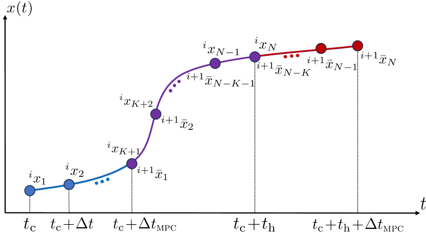
Figure 1: An illustration of the warm-starting procedure. The blue and purple trajectories form the SCP solution at $i$th NMPC run. The purple and red trajectories form the initialization to SCP at $(i+1)$th NMPC run.

The warm-start solution uses $N-K$ nodes of the preceding SCP solution as the initialization for the first $N-K$ nodes of the subsequent SCP call:

$${}^{i+1}\bar{x}_{j} ={}^{i}x_{j+K}$$

$${}^{i+1}\bar{u}_{j} ={}^{i}u_{j+K}$$

for $j\in[1\!:\!N-K]$. The initialization for the control input at the last $K$ nodes is set to the control input at the $(N-K)$th node of the previous SCP solution:

$${}^{i+1}\bar{u}_{N-K+j} ={}^{i}u_{N}$$

for $j\in[1\!:\!K]$. The initialization for the states at the last $K$ nodes is determined by integrating dynamics (12) from the last state of the previous SCP solution with the control inputs at the last $K$ nodes as follows:

$${}^{i+1}\bar{x}_{N-K+j}{}={}^{i}x_{N}+\int_{{t_{\mathrm{c}}}+t_{\mathrm{h}}}^{t_{\mathrm{c}}+t_{\mathrm{h}}+j\Delta t}\!\!\!\!\!f(t,x(t),{}^{i}u_{N})\mathrm{d}t$$

for $j\in[0\!:\!K-1]$. Therefore, if the preceding SCP solution is dynamically feasible, then the initialization for the subsequent SCP call will be dynamically feasible as well. This aspect of warm-starting is crucial for achieving rapid convergence. Due to this rapid convergence facilitated by warm-starting, we terminate SCP prior to complete convergence (similar to the real-time-iteration (RTI) scheme in (Diehl et al., 2005)). We confirm through numerical experiments that premature termination does not compromise the quality of the solutions; however, it notably enhances computational efficiency.

The overall NMPC framework is summarized in Algorithm 1. The inputs to Algorithm 1 comprise the total execution time of NMPC, $T$, the horizon time $t_{\mathrm{h}}$, and grid sizes $N$ and $K$ for defining $\Delta t$ and $\Delta t_{\textsc{mpc}}$, along with an initialization for the first SCP call denoted as:

$${}^{1}\!\bar{Z}=({}^{1}\bar{x}_{1},\ldots,{}^{1}\bar{x}_{N},{}^{1}\bar{u}_{1},\ldots,{}^{1}\bar{u}_{N})$$

Given the maximum number of iterations $j_{\max}$, grid size $N$, current time $t_{\mathrm{c}}$, and time duration $t_{\mathrm{h}}$, we define function $\textsc{scp}_{N,t_{\mathrm{c}},t_{\mathrm{h}}}^{j_{\max}}$, which applies the SCP algorithm described in Section 2.5 to solve (20) with inputs: current state estimate $\hat{x}_{\mathrm{c}}$, running cost function $L$, and path constraint functions $g$ and $h$. Note that the running cost function captures the tracking cost for the current segment of a reference trajectory over $[t_{\mathrm{c}},t_{\mathrm{c}}+t_{\mathrm{h}}]$. Each run of NMPC starts with information acquisition by the sensors, which then provides estimates of the current state, running cost, and constraints, all of which dynamically evolve over time. Then, the SCP call yields a sub-optimal solution for (20), which is also used to warm-start SCP in the subsequent NMPC run. The control input solution from the SCP call is applied to the system until the time instant of the next NMPC run.

Algorithm 1 NMPC Framework

Inputs: $T$, $t_{\mathrm{h}}$, $K$, $N$, $j_{\max}$, ${}^{1}\!\bar{Z}$

$i\leftarrow 0$

$t_{\mathrm{c}}\leftarrow 0$

$\Delta t\leftarrow t_{\mathrm{h}}/(N-1)$

$\Delta t_{\textsc{mpc}}\leftarrow K\Delta t$

while $t_{\mathrm{c}}\leq T$ do

     $\hat{x}(t_{\mathrm{c}}),{}^{i}\!L,{}^{i}\!g,{}^{i}\!h\leftarrow$ sensor($x(t_{\mathrm{c}})$)

     ${}^{i}Z\leftarrow\textsc{scp}_{N,t_{\mathrm{c}},t_{\mathrm{h}}}^{j_{\max}}(\hat{x}(t_{\mathrm{c}}),{}^{i}\!L,{}^{i}\!g,{}^{i}\!h,{}^{i}\!\bar{Z})$

     ${}^{i+1}\bar{Z}\leftarrow$ warm_start$({}^{i}Z)$

     $x(t_{\mathrm{c}}+\Delta t_{\textsc{mpc}})\leftarrow$ evolve($x(t_{\mathrm{c}})$, ${}^{i}\!Z$)

     $i\leftarrow i+1$

     $t_{\mathrm{c}}\leftarrow t_{\mathrm{c}}+\Delta t_{\textsc{mpc}}$

end while

4 Numerical results

This section describes a numerical demonstration of the proposed NMPC framework for output reference tracking, with obstacle avoidance, for a double-integrator with drag and bounded control inputs. The system state is defined as $\xi(t)=(r(t),v(t))$, where $r(t)$ and $v(t)$ are the vehicle’s position and velocity, and the right-hand-side of the governing ODE is given by:

$$F(t,\xi(t),u(t))=\begin{bmatrix}v(t)\\ u(t)-c_{\mathrm{d}}\|v(t)\|v(t)\end{bmatrix}$$

where $c_{\mathrm{d}}$ is the drag coefficient of the vehicle.

The running cost is defined as:

$$L(t,\xi(t),u(t))=\|r(t)-r_{\mathrm{ref}}(t)\|^{2}$$

where $r_{\mathrm{ref}}$ is the reference output. We assume that the vehicle has a sensor, such as a LiDAR, that detects the obstacle within a range denoted by $r_{\mathrm{sens}}\in\mathbb{R}_{+}$. We include the instantaneously detected obstacles to (12) at each NMPC run. We assume that the obstacles are elliptical and define an index set of the obstacles that are detected by the sensor at time $t_{\mathrm{c}}$ as:

$$\mathcal{O}_{\mathrm{c}}=\{i\mid\|S^{i}(r(t_{\mathrm{c}})-r^{i}_{\mathrm{obs}})\|\leq r_{\mathrm{sens}},~{}i\in[1\!:\!n_{\mathrm{obs}}]\}$$

where $n_{\mathrm{obs}}$ is the total number of the obstacles, $S^{i}$ is the shape matrix of $i$th obstacle, $r_{\mathrm{obs}}$ is a matrix such that the $i$th column of the matrix, $r^{i}_{\mathrm{obs}}$, represents the center of the $i$th obstacle. The vector-valued path constraint function, which includes the obstacle avoidance constraints, is given by:

$$g(t,\xi(t),u(t))=\begin{bmatrix}\vdots\\ 1-\|S^{i}(r(t)-r^{i}_{\mathrm{obs}})\|\\ \vdots\end{bmatrix},~{}\forall i\in\mathcal{O}_{\mathrm{c}}$$

The boundary condition defined for CTCS in (13) is relaxed by $\epsilon>0$ in (19) to satisfy LICQ. However, this relaxation may cause a pointwise violation of the constraint. In (Elango et al., 2024), it is proved that for each relaxation parameter $\epsilon>0$, there exists a constraint tightening value $\delta_{\textrm{obs}}>0$ such that

$$\int_{t_{k}}^{t_{k+1}}|g_{i}(t,\xi(t),u(t))+\delta_{\textrm{obs}}|_{+}^{2}\mathrm{d}t\leq\epsilon$$

$$\iff\int_{t_{k}}^{t_{k+1}}|g_{i}(t,\xi(t),u(t))|_{+}^{2}\mathrm{d}t=0$$

The choice of constraint tightening value $\delta_{\textrm{obs}}$ is determined by the results of numerical experiments.

Note that the obstacle avoidance constraint function is not differentiable at $0$, specifically when the vehicle’s position coincides with the center point of the obstacle. However, this situation is not typically expected to occur unless the initialization is intentionally configured this way. If this situation presents an issue, we can address it by using a smooth quadratic in place of the norm.

Convex constraints on the control input are encoded by $\mathcal{U}=\{u\in\mathbb{R}^{2}\,|\,\|u\|\leq u_{\max}\}$. Table 1 shows the system and simulation parameters.

Table 1:

Parameter	Value
$T$, $t_{\mathrm{h}}$, $K$, $N$, $j_{\mathrm{max}}$	$30$ s, $8$ s, $4$, $17$, $3$
$u_{\max}$	$5$ m s-2
$c_{\mathrm{d}}$	$0.05$ m-1
$r_{\mathrm{ref}}(t)$	$\left[\begin{array}[]{c}-10+2t/3\\ 5e^{-0.05t}\sin\left(\pi/2+t/5+t^{2}/36\right)\end{array}\right]$
$S^{i}$, $i=1,\dots,5$	$\left[\begin{array}[]{cc}2.4&0\\ 0&0.4\end{array}\right]$
$r_{\mathrm{obs}}$	$\left[\begin{array}[]{cccccccccc}-6.5&-1.8&0.5&2.7&6.2\\ -3&3.5&-3.5&1.5&-3\end{array}\right]$
$\delta_{\textrm{obs}}$	$0.05$
$r_{\mathrm{sens}}$	$6$ m

We study the impact of premature termination on the quality of the solution. Within each NMPC run, we run SCP for $10$ iterations, and in each SCP iteration, we record the values of the $J_{l}$, $J_{y}$, and $J_{\mathrm{prox}}$ terms defined in (25). When these quantities converge to the chosen convergence tolerance, it indicates that the integral of the running cost in the reformulated problem is accurate, the obstacle avoidance constraint is satisfied, and the overall convergence of SCP.

Figure 2 shows the variation in the mean and standard deviation of the values of these quantities along the trajectory as a function of the number of SCP iterations. These plots indicate that terminating SCP after $3$ iterations yields an acceptable solution.

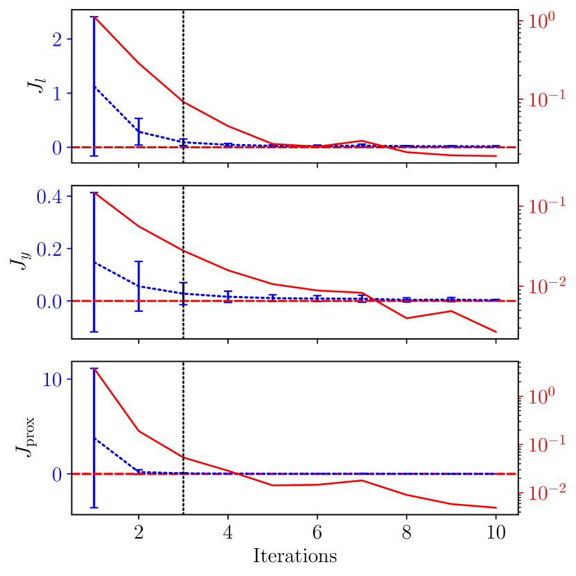
Figure 2: The mean and standard deviation of $J_{l}$, $J_{y}$, and $J_{\mathrm{prox}}$ along the trajectory for $10$ SCP iterations. The linear scale on the left axis corresponds to the mean and standard deviation shown by the blue curve, while the log scale on the right axis corresponds to the mean shown by the red curve. The black-dashed line denotes the iteration at which the SCP algorithm is set to terminate.

We compare the proposed approach against the usual method of considering only the node point state and control inputs, in order to quantify the integral of the running cost and violation of the obstacle avoidance constraint. The output reference tracking and obstacle avoidance results are shown in Figures 3 and 4.

Figure 3 indicates that in the node-only case, the obstacle avoidance constraint is not satisfied for the continuous-time trajectory (obtained via a single shooting propagation of the system dynamics with the NMPC control input), despite being satisfied at all node points. Conversely, the CTCS formulation ensures that the constraint is satisfied at all times along the trajectory.

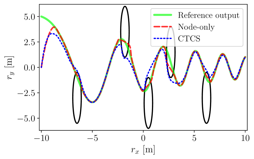
Figure 3: $r_{x}$ and $r_{y}$ represent the first and second components of the position vector $r$, respectively. A green solid curve illustrates the reference output, while black ellipses represent the obstacles. The trajectories obtained from NMPC using the node-only and the CTCS formulations are presented as red-dashed and blue-dotted curves, respectively.

Figure 4 demonstrates that both the node-only and CTCS formulations exhibit comparable performances in terms of output reference tracking. The CTCS formulation shows a slightly lower performance, but this difference is because the CTCS formulation actually satisfies the obstacle avoidance constraint.

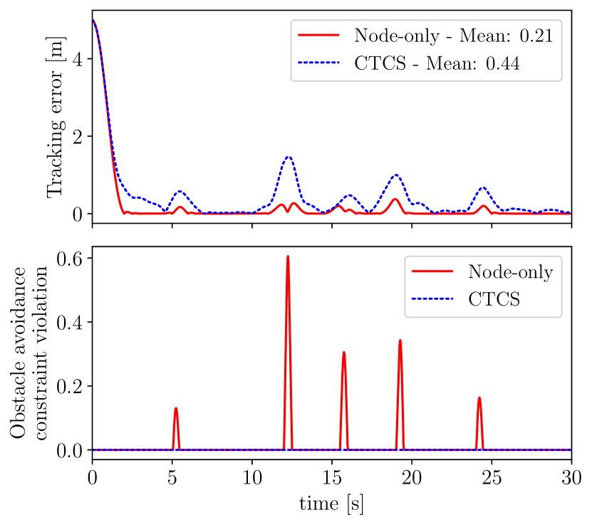
Figure 4: The first plot shows the discrepancy between the reference output and the trajectories obtained from NMPC using the node-only and the CTCS formulations throughout the simulation. The legend reports the average discrepancy over the entire simulation. The second plot shows the violation in the obstacle avoidance constraint, quantified by $1^{\top}|g(t,\xi(t),u(t))|_{+}$, throughout the simulation.

5 Conclusions

This paper presents the adaptation of a successive convexification framework to address the NMPC problem. Reformulating the optimal control problem by embedding path constraints and the running cost into the dynamics function within the successive convexification framework offers the benefit of being able to operate on sparse discretization grids without encountering inter-sample constraint violations or a degradation in the accuracy of the running cost. The prox-linear method, a convergence-guaranteed SCP algorithm that requires only first-order information and supports warm-starting, is employed to solve the reformulated optimal control problem. The aforementioned attributes allow the algorithm to operate in an RTI-like mode while achieving a favorable solution in a few iterations and maintaining real-time capability. The proposed framework is demonstrated on a tracking problem involving obstacle avoidance.

References

- ApS (2019) ApS, M. (2019). MOSEK optimization toolbox for MATLAB. User’s Guide and Reference Manual, Version, 4(1). URL https://docs.mosek.com/10.1/toolbox.pdf.
- Bock and Plitt (1984) Bock, H.G. and Plitt, K.J. (1984). A multiple shooting algorithm for direct solution of optimal control problems. IFAC proceedings volumes, 17(2), 1603–1608. URL https://doi.org/10.1016/s1474-6670(17)61205-9.
- Chari et al. (2024) Chari, G.M., Kamath, A.G., Elango, P., and Açıkmeşe, B. (2024). Fast monte carlo analysis for 6-DoF powered-descent guidance via GPU-accelerated sequential convex programming. In AIAA SciTech 2024 Forum. AIAA. URL https://doi.org/10.2514/6.2024-1762.
- Di Cairano et al. (2013) Di Cairano, S., Bernardini, D., Bemporad, A., and Kolmanovsky, I.V. (2013). Stochastic MPC with learning for driver-predictive vehicle control and its application to HEV energy management. IEEE Transactions on Control Systems Technology, 22(3), 1018–1031. URL https://doi.org/10.1109/TCST.2013.2272179.
- Diamond and Boyd (2016) Diamond, S. and Boyd, S. (2016). CVXPY: A Python-embedded modeling language for convex optimization. Journal of Machine Learning Research, 17(83), 1–5. URL https://www.cvxpy.org/.
- Diehl et al. (2005) Diehl, M., Bock, H.G., and Schlöder, J.P. (2005). A real-time iteration scheme for nonlinear optimization in optimal feedback control. SIAM Journal on Control and Optimization, 43(5), 1714–1736. URL https://doi.org/10.1137/S0363012902400713.
- Dinh et al. (2012) Dinh, Q.T., Savorgnan, C., and Diehl, M. (2012). Adjoint-based predictor-corrector sequential convex programming for parametric nonlinear optimization. SIAM Journal on Optimization, 22(4), 1258–1284. URL https://doi.org/10.1137/110844349.
- Domahidi et al. (2013) Domahidi, A., Chu, E., and Boyd, S. (2013). ECOS: An SOCP solver for embedded systems. In 2013 European control conference (ECC), 3071–3076. IEEE. URL https://doi.org/10.23919/ECC.2013.6669541.
- Drusvyatskiy and Lewis (2018) Drusvyatskiy, D. and Lewis, A.S. (2018). Error bounds, quadratic growth, and linear convergence of proximal methods. Mathematics of Operations Research, 43(3), 919–948. URL https://doi.org/10.1287/moor.2017.0889.
- Elango et al. (2022) Elango, P., Kamath, A., Yu, Y., Carson III, J.M., and Açıkmeşe, B. (2022). A customized first-order solver for real-time powered-descent guidance. In AIAA SCITECH 2022 Forum. American Institute of Aeronautics and Astronautics. URL https://doi.org/10.2514/6.2022-0951.
- Elango et al. (2024) Elango, P., Luo, D., Kamath, A.G., Uzun, S., Kim, T., and Açıkmeşe, B. (2024). Successive convexification for trajectory optimization with continuous-time constraint satisfaction. arXiv preprint arXiv:2404.16826. URL https://doi.org/10.48550/arXiv.2404.16826.
- Eren et al. (2017) Eren, U., Prach, A., Koçer, B.B., Raković, S.V., Kayacan, E., and Açıkmeşe, B. (2017). Model predictive control in aerospace systems: Current state and opportunities. Journal of Guidance, Control, and Dynamics, 40(7), 1541–1566. URL https://doi.org/10.2514/1.G002507.
- Fontes and Paiva (2019) Fontes, F.A.C.C. and Paiva, L.T. (2019). Guaranteed constraint satisfaction in continuous-time control problems. IEEE Control Systems Letters, 3(1), 13–18. URL http://dx.doi.org/10.1109/LCSYS.2018.2849853.
- Frank Allgöwer (2000) Frank Allgöwer, A.Z. (2000). Nonlinear Model Predictive Control. Birkhäuser Basel. URL https://doi.org/10.1007/978-3-0348-8407-5.
- Frison and Diehl (2020) Frison, G. and Diehl, M. (2020). HPIPM: a high-performance quadratic programming framework for model predictive control. IFAC-PapersOnLine, 53(2), 6563–6569. URL https://doi.org/10.1016/J.IFACOL.2020.12.073.
- Gros et al. (2020) Gros, S., Zanon, M., Quirynen, R., Bemporad, A., and Diehl, M. (2020). From linear to nonlinear MPC: bridging the gap via the real-time iteration. International Journal of Control, 93(1), 62–80. URL https://doi.org/10.1080/00207179.2016.1222553.
- Gruber and Althoff (2021) Gruber, F. and Althoff, M. (2021). Scalable robust output feedback MPC of linear sampled-data systems. In 2021 60th IEEE Conference on Decision and Control (CDC). IEEE. URL http://dx.doi.org/10.1109/CDC45484.2021.9683384.
- Henson (1998) Henson, M.A. (1998). Nonlinear model predictive control: current status and future directions. Computers & Chemical Engineering, 23(2), 187–202. URL http://dx.doi.org/10.1016/S0098-1354(98)00260-9.
- Houska et al. (2011) Houska, B., Ferreau, H.J., and Diehl, M. (2011). An auto-generated real-time iteration algorithm for nonlinear MPC in the microsecond range. Automatica, 47(10), 2279–2285. URL https://doi.org/10.1016/j.automatica.2011.08.020.
- Jackson et al. (2021) Jackson, B.E., Punnoose, T., Neamati, D., Tracy, K., Jitosho, R., and Manchester, Z. (2021). ALTRO-C: A fast solver for conic model-predictive control. In 2021 IEEE International Conference on Robotics and Automation (ICRA), 7357–7364. IEEE. URL https://doi.org/10.1109/ICRA48506.2021.9561438.
- Kamath et al. (2023a) Kamath, A.G., Elango, P., Mceowen, S., Yu, Y., Carson III, J.M., Mesbahi, M., and Açıkmeşe, B. (2023a). Customized real-time first-order methods for onboard dual quaternion-based 6-DoF powered-descent guidance. In AIAA SCITECH 2023 Forum. American Institute of Aeronautics and Astronautics. URL https://doi.org/10.2514/6.2023-2003.
- Kamath et al. (2023b) Kamath, A.G., Elango, P., Yu, Y., Mceowen, S., Chari, G.M., Carson, III, J.M., and Açıkmeşe, B. (2023b). Real-time sequential conic optimization for multi-phase rocket landing guidance. IFAC-PapersOnLine, 56(2), 3118–3125. URL https://doi.org/10.1016/j.ifacol.2023.10.1444.
- Kim et al. (2002) Kim, H.J., Shim, D.H., and Sastry, S. (2002). Nonlinear model predictive tracking control for rotorcraft-based unmanned aerial vehicles. In Proceedings of the 2002 American Control Conference, volume 5, 3576–3581. IEEE. URL https://doi.org/10.1109/ACC.2002.1024483.
- Liberzon (2011) Liberzon, D. (2011). Calculus of Variations and Optimal Control Theory: A Concise Introduction. Princeton University Press. URL https://doi.org/10.2307/j.ctvcm4g0s.
- Magni and Scattolini (2004) Magni, L. and Scattolini, R. (2004). Model predictive control of continuous-time nonlinear systems with piecewise constant control. IEEE Transactions on Automatic Control, 49(6), 900–906. URL http://dx.doi.org/10.1109/TAC.2004.829595.
- Malyuta et al. (2022) Malyuta, D., Reynolds, T.P., Szmuk, M., Lew, T., Bonalli, R., Pavone, M., and Açıkmeşe, B. (2022). Convex optimization for trajectory generation: A tutorial on generating dynamically feasible trajectories reliably and efficiently. IEEE Control Systems Magazine, 42(5), 40–113. URL https://doi.org/10.1109/MCS.2022.3187542.
- Malyuta et al. (2019) Malyuta, D., Reynolds, T.P., Szmuk, M., Mesbahi, M., Açıkmeşe, B., and Carson III, J.M. (2019). Discretization performance and accuracy analysis for the rocket powered descent guidance problem. In AIAA SciTech 2019 Forum. Reston, Virginia. URL https://doi.org/10.2514/6.2019-0925.
- Malyuta et al. (2021) Malyuta, D., Yu, Y., Elango, P., and Açıkmeşe, B. (2021). Advances in trajectory optimization for space vehicle control. Annual Reviews in Control, 52, 282–315. URL https://doi.org/10.1016/j.arcontrol.2021.04.013.
- Mao et al. (2019) Mao, Y., Dueri, D., Szmuk, M., and Açıkmeşe, B. (2019). Convexification and real-time optimization for MPC with aerospace applications. Handbook of Model Predictive Control, 335–358. URL https://doi.org/10.1007/978-3-319-77489-3_15.
- Mayne (1973) Mayne, D.Q. (1973). Differential dynamic programming—a unified approach to the optimization of dynamic systems. In Control and Dynamic Systems, volume 10, 179–254. Elsevier. URL https://doi.org/10.1016/B978-0-12-012710-8.50010-8.
- Messerer et al. (2021) Messerer, F., Baumgärtner, K., and Diehl, M. (2021). Survey of sequential convex programming and generalized Gauss-Newton methods. ESAIM: Proceedings and Surveys, 71, 64–88. URL https://doi.org/10.1051/proc/202171107.
- Mitchell and Kaynama (2015) Mitchell, I.M. and Kaynama, S. (2015). An improved algorithm for robust safety analysis of sampled data systems. In Proceedings of the 18th International Conference on Hybrid Systems: Computation and Control, HSCC ’15. ACM. URL http://dx.doi.org/10.1145/2728606.2728619.
- Morgan et al. (2014) Morgan, D., Chung, S.J., and Hadaegh, F.Y. (2014). Model predictive control of swarms of spacecraft using sequential convex programming. Journal of Guidance, Control, and Dynamics, 37(6), 1725–1740. URL https://doi.org/10.2514/1.G000218.
- Nocedal and Wright (2006) Nocedal, J. and Wright, S. (2006). Numerical Optimization. Springer, 2 edition. URL https://doi.org/10.1007/978-0-387-40065-5.
- Quirynen et al. (2015a) Quirynen, R., Vukov, M., and Diehl, M. (2015a). Multiple shooting in a microsecond. In Multiple Shooting and Time Domain Decomposition Methods: MuS-TDD, Heidelberg, May 6-8, 2013, 183–201. Springer. URL https://doi.org/10.1007/978-3-319-23321-5_7.
- Quirynen et al. (2015b) Quirynen, R., Vukov, M., Zanon, M., and Diehl, M. (2015b). Autogenerating microsecond solvers for nonlinear MPC: a tutorial using ACADO integrators. Optimal Control Applications and Methods, 36(5), 685–704. URL https://doi.org/10.1002/oca.2152.
- Rawlings et al. (2017) Rawlings, J.B., Mayne, D.Q., and Diehl, M. (2017). Model Predictive Control: Theory, Computation, and Design, volume 2. Nob Hill Publishing Madison, WI. URL https://sites.engineering.ucsb.edu/~jbraw/mpc/.
- Reynolds et al. (2020) Reynolds, T.P., Malyuta, D., Mesbahi, M., Açıkmeşe, B., and Carson III, J.M. (2020). A real-time algorithm for non-convex powered descent guidance. In AIAA SciTech 2020 Forum, 1–24. URL https://doi.org/10.2514/6.2020-0844.
- Sadraddini and Tedrake (2020) Sadraddini, S. and Tedrake, R. (2020). Robust output feedback control with guaranteed constraint satisfaction. In Proceedings of the 23rd International Conference on Hybrid Systems: Computation and Control, HSCC ’20. ACM. URL http://dx.doi.org/10.1145/3365365.3382211.
- Sargent and Sullivan (1978) Sargent, R. and Sullivan, G. (1978). The development of an efficient optimal control package. In Optimization Techniques: Proceedings of the 8th IFIP Conference on Optimization Techniques Würzburg, September 5–9, 1977, 158–168. Springer. URL https://doi.org/10.1007/BFb0006520.
- Schlipf et al. (2012) Schlipf, D., Schlipf, D.J., and Kühn, M. (2012). Nonlinear model predictive control of wind turbines using LIDAR. Wind Energy, 16(7), 1107–1129. URL https://doi.org/10.1002/we.1533.
- Szmuk et al. (2020) Szmuk, M., Reynolds, T.P., and Açıkmeşe, B. (2020). Successive convexification for real-time six-degree-of-freedom powered descent guidance with state-triggered constraints. Journal of Guidance, Control, and Dynamics, 43(8), 1399–1413. URL http://dx.doi.org/10.2514/1.G004549.
- Tassa et al. (2012) Tassa, Y., Erez, T., and Todorov, E. (2012). Synthesis and stabilization of complex behaviors through online trajectory optimization. In 2012 IEEE/RSJ International Conference on Intelligent Robots and Systems, 4906–4913. IEEE. URL https://doi.org/10.1109/IROS.2012.6386025.
- Tassa et al. (2014) Tassa, Y., Mansard, N., and Todorov, E. (2014). Control-limited differential dynamic programming. In 2014 IEEE International Conference on Robotics and Automation (ICRA), 1168–1175. IEEE. URL https://doi.org/10.1109/ICRA.2014.6907001.
- Wanner and Hairer (1996) Wanner, G. and Hairer, E. (1996). Solving Ordinary Differential Equations II, volume 375. Springer Berlin Heidelberg New York. URL https://doi.org/10.1007/978-3-642-05221-7.
- Weiss and Di Cairano (2014) Weiss, A. and Di Cairano, S. (2014). Robust dual control MPC with guaranteed constraint satisfaction. In 53rd IEEE Conference on Decision and Control. IEEE. URL http://dx.doi.org/10.1109/CDC.2014.7040443.
- Xie et al. (2019) Xie, S., Hu, X., Xin, Z., and Brighton, J. (2019). Pontryagin’s minimum principle based model predictive control of energy management for a plug-in hybrid electric bus. Applied Energy, 236, 893–905. URL https://doi.org/10.1016/j.apenergy.2018.12.032.
- Yu et al. (2022a) Yu, Y., Elango, P., Açıkmeşe, B., and Topcu, U. (2022a). Extrapolated proportional-integral projected gradient method for conic optimization. IEEE Control Systems Letters, 7, 73–78. URL https://doi.org/10.1109/LCSYS.2022.3186647.
- Yu et al. (2022b) Yu, Y., Elango, P., Topcu, U., and Açıkmeşe, B. (2022b). Proportional–integral projected gradient method for conic optimization. Automatica, 142, 110359. URL https://doi.org/10.1016/j.automatica.2022.110359.
- Zeilinger et al. (2014) Zeilinger, M.N., Raimondo, D.M., Domahidi, A., Morari, M., and Jones, C.N. (2014). On real-time robust model predictive control. Automatica, 50(3), 683–694. URL http://dx.doi.org/10.1016/j.automatica.2013.11.019.