Microstructural and Transport Characteristics of Triply Periodic Bicontinuous Materials

Abstract

3D bicontinuous two-phase materials are increasingly gaining interest because of their unique multifunctional characteristics and advancements in techniques to fabricate them. Because of their complex topological and structural properties, it still has been nontrivial to develop explicit microstructure-dependent formulas to predict accurately their physical properties. A primary goal of the present paper is to ascertain various microstructural and transport characteristics of five different models of triply periodic bicontinuous porous materials at a porosity $\phi_{1}=1/2$: those in which the two-phase interfaces are the Schwarz P, Schwarz D and Schoen G minimal surfaces as well as two different pore-channel structures. We ascertain their spectral densities, pore-size distribution functions, local volume-fraction variances, and hyperuniformity order metrics and then use this information to estimate certain effective steady-state as well as time-dependent transport properties via closed-form microstructure-property formulas. Specifically, the recently introduced time-dependent diffusion spreadability is determined exactly from the spectral density. Moreover, we accurately estimate the fluid permeability of such porous materials from a closed-form formula that depends on the second moment of the pore-size function and the formation factor, a measure of the tortuosity of the pore space, is exactly obtained for the three minimal-surface structures. We also rigorously bound the permeability from above using the spectral density. For the five models with identical cubic unit cells, we find that the permeability, inverse of the specific surface, hyperuniformity order metric, pore-size second moment and long-time spreadability behavior are all positively correlated and rank order the structures in exactly the same way. We also conjecture what structures maximize the fluid permeability for arbitrary porosities and show that this conjecture must be true in the extreme porosity limits by identifying the corresponding optimal structures.

url]http://chemlabs.princeton.edu/torquato/

1 Introduction

Two-phase heterogeneous materials (media) abound in Nature and synthetic situations. Examples of such materials include composites and porous media, biological media, foams, polymer blends, granular media, cellular solids, geological media, and colloids [1, 2, 3, 4]. It is well-established that the effective properties of composites generally depend on an infinite set of correlation functions that fully characterize the microstructure [1]. Since such complete information is generally not available, it is useful to devise estimates of the effective properties that depend on nontrivial microstructural information, including accurate approximation formulas [1] and rigorous bounds [1, 2]. Concerning the latter approach, it is well known that the microstructures that maximize or minimize the effective electrical (thermal) conductivities as well as bulk moduli of macroscopically isotropic two-phase composites at a fixed volume fraction consist of a topologically disconnected phase dispersed throughout a continuous (percolating) matrix phase [1, 2]. These extremal structures include the Hashin-Shtrikman sphere assemblages [5], certain laminates [6, 7] and Vigdergauz constructions [8].

It is common for two-phase media to be bicontinuous in three-dimensional Euclidean space $\mathbb{R}^{3}$. A bicontinuous composite is one in which both phases of a two-phase composite are topologically connected across the sample. This topological feature, i.e., percolation of both phases, is rare in two dimensions, while very common in three dimensions [1]. Bicontinuous media that are periodic in three dimensions, i.e., triply periodic, are an important class of two-phase media. They are increasingly gaining interest because of their desirable physical properties and a capacity to readily fabricate them due to advancements in additive manufacturing [9]. Within this class, it has been shown that certain triply periodic minimal surfaces are optimal for several types of multifunctional performance [10, 11, 12, 13, 14]. Triply periodic minimal surfaces in $\mathbb{R}^{3}$ [15, 16, 17, 18, 19], which arise in a multitude of physical [20, 21, 22, 23] and biological contexts [24, 25, 26, 23], are those in which the mean curvature Examples of such surfaces include the Schwarz primitive (P), the Schwarz diamond (D), and the Schoen gyroid (G) surfaces within their fundamental periodic cells are shown in Fig. 1, among other triply periodic bicontinuous media that we consider in this paper, namely, “pore-channel” models. The triply periodic minimal surfaces shown in Fig. 1 partition space into two disjoint but intertwining regions that are simultaneously continuous in which the phase volume fractions $\phi_{1}$ and $\phi_{2}$ are identical, i.e., $\phi_{1}=\phi_{2}=1/2$. In A, we show that the domains of both percolating phases in the P, D, and G minimal surfaces are identical up to simple translation and reflection transformations, implying that they obey statistical phase-inversion symmetry.

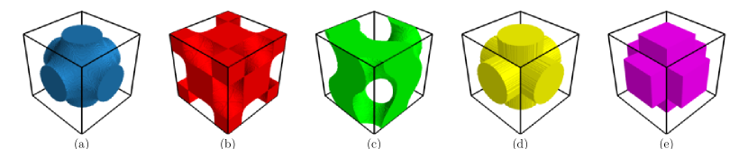
Figure 1: Fundamental (unit) cells of phase 1 domains for the five triply periodic models with porosity $\phi_{1}=0.5$ that are considered in this work: (a) Schwarz P, (b) Schwarz D, (c) Schoen G, (d) spherical-pore/circular-channel model, and (e) cubic-pore/square-channel model. For each of the three triply periodic minimal surfaces (a-c), the domains of both percolating phases are identical up to simple translation and reflection transformations, implying that they obey statistical phase-inversion symmetry; see A. The general spherical-pore/circular-channel model has a single spherical pore of radius $a+b$ and three perpendicular cylindrical channels of radius $a$, which intersect at the center of the fundamental cell; see Ref. [13, 14]. Analogously, the general cubic-pore/square-channel model consists of a cubic pore of side length $2(a+b)$ and three square channels of side length $2a$. We study these two pore-channel models with $b=0$, called the circular- and square-channel models.

It has been demonstrated that triply periodic two-phase bicontinuous composites with interfaces that are the Schwarz P and D minimal surfaces are not only geometrically extremal but extremal when heat transport competes with electrical transport of heat and electricity [10, 11]. More specifically, these triply periodic minimal surfaces maximize the values of the sum of the effective thermal conductivity $\lambda_{e}$ and electrical conductivity $\sigma_{e}$ of three-dimensional two-phase composites at 50% volume fraction with symmetric “ill-ordered” phases, i.e., when the heat conductivity phase contrast ratio is the inverse of the electrical conductivity phase contrast ratio. Moreover, such triply periodic composites have also been discovered to be optimal for certain multifunctional bulk modulus and electrical conductivity optimizations [12].

Furthermore, the macroscopically isotropic porous medium with the Schwarz P interface, where phase 1 is the pore phase and hence has a porosity $\phi_{1}=1/2$, was found to have the largest fluid permeability $\mathbbm{k}$ [13] as well as the largest mean survival time $\tau$ [14], among a wide class of triply periodic porous media that were examined in these studies. The former study led to the following conjecture:

Conjecture 1

Among three-dimensional porous media at porosity $\phi_{1}=1/2$ within a simple cubic fundamental cell of side length $L$ under periodic boundary conditions, the dimensionless isotropic fluid permeability $\mathbbm{k}/L^{2}$ is maximized for the structure that minimizes the total interface area, which is proposed to be the Schwarz primitive (P) minimal surface [13].

Subsequently, strong numerical evidence (using level-set methods) was provided to support the proposition that the Schwarz P surface is the structure that minimizes the total interface area [18].

Due to the complexity of the topological and structural properties of triply periodic bicontinuous materials, it has been nontrivial to develop explicit microstructure-dependent formulas that enable accurate predictions of their physical properties. Given the importance of this class of materials, a primary goal of the present paper is to ascertain various microstructural characteristics, including the spectral densities, pore-size distribution functions, local volume-fraction fluctuations, and the associated hyperuniformity order metrics for the structures shown in Fig. 1. Some of this microstructural information is then used to estimate certain effective steady-state as well as time-dependent transport properties via closed-form microstructure-property formulas. The steady-state properties examined are the macroscopically isotropic fluid permeability $\mathbbm{k}$ and the effective electrical conductivity $\sigma_{e}$ We also determine the recently introduced time-dependent diffusion spreadability ${\cal S}(t)$ as a function of time $t$. Importantly, among these physical properties, the most challenging to predict theoretically for general microstructures is the fluid permeability $\mathbbm{k}$, which is defined by Darcy’s law [27, 1, 3]. We also generalize Conjecture 1 for $\phi_{1}=1/2$ to include the structures that maximize the fluid permeability for arbitrary porosities, and then show that this generalized conjecture must be true in the extreme porosity limits ($\phi_{1}$ tending to zero and to unity) by identifying the corresponding optimal structures.

In Sec. 2, we present pertinent background/definitions of the microstructural descriptors and hyperuniformity concept. In Sec. 3, explicit formulas that relate transport properties to the microstructure are provided and discussed, including the derivation of a formula for the effective conductivity $\sigma_{e}$ that applies to general bicontinuous media, which reduces to an exact for $\sigma_{e}$ for the triply periodic minimal surfaces and is an excellent approximation for $\sigma_{e}$ of general bicontinuous media for $\phi_{1}$ in the vicinity of $1/2$. We also provide relevant known formulas for the fluid permeability and the spreadability that are functionals of certain statistical descriptors, which are computed in Sec. 4. In Sec. 5, we apply the microstructure-dependent formulas of Sec. 3 and results of Sec. 4 to predict the aforementioned transport properties of the five triply periodic bicontinuous models shown in Fig. 1. In Sec. 6, we generalize Conjecture 1 to include the structures that maximize the permeability for all nontrivial porosities, i.e., $0<\phi_{1}<1$. Finally, in Sec. 7, we remark on how the various structural and physical properties of the five triply periodic media models studied here are positively correlated with one another. We also describe open problems.

2 Background on Microstructural Descriptors and Hyperuniformity

There are a multitude of different statistical descriptors of the microstructure of two-phase media; see Ref. [1] and references therein. The most relevant for the purposes of this paper are the $n$-point correlation functions, spectral density, pore-size distributions, local volume-fraction fluctuations, and hyperuniformity characteristics, which are defined below and applied in subsequent sections.

2.1 $n$-Point Correlation Functions

A two-phase random medium is a domain of space $\mathcal{V}\subseteq\mathbb{R}^{d}$ that is partitioned into two disjoint regions that make up $\mathcal{V}$: a phase 1 region $\mathcal{V}_{1}$ of volume fraction $\phi_{1}$ and a phase 2 region $\mathcal{V}_{2}$ of volume fraction $\phi_{2}$ [1]. The phase indicator function $\mathcal{I}^{(i)}(\mathbf{x};\omega)$ for a given realization $\omega$ is defined as

$$\mathcal{I}^{(i)}(\mathbf{x};\omega)\equiv\begin{cases}1,&\mathbf{x}\in\mathcal{V}_{i},\\ 0,&\mathbf{x}\notin\mathcal{V}_{i},\end{cases}\qquad(i=1,2).$$ (1)

The statistical properties of each phase of the system are specified by the countably infinite set of $n$-point correlation functions $S_{n}^{(i)}$, which are defined by [28, 29, 1]:

$$S_{n}^{(i)}(\mathbf{x}_{1},\ldots,\mathbf{x}_{n})\equiv\left\langle\prod_{i=1}^{n}{\cal I}^{(i)}(\mathbf{x}_{j};\omega)\right\rangle,$$ (2)

where angular brackets denote an ensemble average over realizations. The $n$-point correlation function $S_{n}^{(i)}(\mathbf{x}_{1},\ldots,\mathbf{x}_{n})$ has a probabilistic interpretation: it gives the probability of finding the ends of the vectors $\mathbf{x}_{1},\ldots,\mathbf{x}_{n}$ all in phase $i$. For this reason, $S_{n}^{(i)}(\mathbf{x}_{1},\ldots,\mathbf{x}_{n})$ is sometimes referred to as the $n$-point probability function.

If the medium is statistically homogeneous, $S_{n}^{(i)}(\mathbf{x}_{1},\ldots,\mathbf{x}_{n})$ is translationally invariant and, in particular, the one-point correlation function is independent of position and equal to the volume fraction of phase $i$:

$$S_{1}^{(i)}(\mathbf{x})=\phi_{i},$$ (3)

while the two-point correlation function $S_{2}^{(i)}({\bf r})$ depends on the displacement vector ${\bf r}\equiv\mathbf{x}_{2}-\mathbf{x}_{1}$.

For statistically homogeneous media, the autocovariance function $\mathinner{\chi_{{}_{V}}\mathopen{\left(\bm{r}\right)}}$ can be defined in terms of the mean-zero fluctuating indicator function,

$$\mathinner{\mathcal{J}^{(i)}\mathopen{\left(\bm{r}\right)}}\equiv\mathinner{\mathcal{I}^{(i)}\mathopen{\left(\bm{r}\right)}}-\phi_{i},$$ (4)

as follows [1]:

$$\mathinner{\chi_{{}_{V}}\mathopen{\left(\bm{r}\right)}}\equiv\langle{\mathinner{\mathcal{J}^{(i)}\mathopen{\left(\bm{r}^{\prime}\right)}}\mathinner{\mathcal{J}^{(i)}\mathopen{\left(\bm{r}^{\prime}+\bm{r}\right)}}}\rangle,$$ (5)

which is identical for each phase. At the extreme limits of its argument, $\chi_{{}_{V}}$ has the following asymptotic behaviors:

$$\chi_{{}_{V}}({\bf r}=0)=\phi_{1}\phi_{2},\qquad\lim_{|{\bf r}|\rightarrow\infty}\chi_{{}_{V}}({\bf r})=0,$$ (6)

in which the latter limit applies when the medium possesses no long-range order. If the medium is statistically homogeneous and isotropic, then ${\chi}_{{}_{V}}({\bf r})$ depends only on the magnitude of its argument $r=|\bf r|$, and hence is a radial function. In such instances, its slope at the origin is directly related to the specific surface $s$ (interface area per unit volume); specifically, we have in any space dimension $d$, the small-$r$ asymptotic form [1],

$$\chi_{{}_{V}}({\bf r})=\phi_{1}\phi_{2}-\beta(d)s\;|{\bf r}|+{\cal O}(|{\bf r}|^{2}),$$ (7)

where

$$\beta(d)=\frac{\Gamma(d/2)}{2\sqrt{\pi}\Gamma((d+1)/2)}$$ (8)

and $\Gamma(x)$ is the gamma function.

2.2 Spectral Density

A microstructural quantity of key interest in this paper is the spectral density ${\tilde{\chi}}_{{}_{V}}({\bf k})$, which is the Fourier transform of $\chi_{{}_{V}}({\bf r})$, i.e.,

$${\tilde{\chi}}_{{}_{V}}({\bf k})=\int_{\mathbb{R}^{d}}\chi_{{}_{V}}({\bf r})\,e^{-i{\bf k\cdot r}}{\rm d}{\bf r}\geq 0,\qquad\mbox{for all}\;{\bf k}.$$ (9)

It is a  nonnegative function for all wavevectors $\bf k$ and can be obtained experimentally from scattering intensity measurements [30, 31]. For a general statistically homogeneous two-phase medium, the spectral density must obey the following sum rule [1, 32]:

$$\frac{1}{(2\pi)^{d}}\int_{\mathbb{R}^{d}}{\tilde{\chi}}_{{}_{V}}({\bf k})\,d{\bf k}=\chi_{{}_{V}}({\bf r}=0)=\phi_{1}\phi_{2}.$$ (10)

This follows immediately from the Fourier representation of the autocovariance function, i.e.,

$$\chi_{{}_{V}}({\bf r})=\frac{1}{(2\pi)^{d}}\int_{\mathbb{R}^{d}}{\tilde{\chi}}_{{}_{V}}({\bf k})\,e^{i{\bf k\cdot r}}{\rm d}{\bf k}.$$ (11)

For statistically isotropic media, the spectral density only depends on the wavenumber $k=|{\bf k}|$ and, as a consequence of Eq. (7), its decay in the large-$k$ limit is controlled by the following exact power-law form:

$${\tilde{\chi}}_{{}_{V}}({\bf k})\sim\frac{\gamma(d)\,s}{k^{d+1}},\qquad k\rightarrow\infty,$$ (12)

where $s$ is the specific surface and

$$\gamma(d)=2^{d}\,\pi^{(d-1)/2}\,\Gamma((d+1)/2)\,\beta(d)$$ (13)

is a $d$-dimensional constant and $\beta(d)$ is given by (8).

2.3 Volume-Fraction Fluctuations and Hyperuniformity

A hyperuniform point configuration in $d$-dimensional Euclidean space $\mathbb{R}^{d}$ is one in which there is an anomalous suppression of large-scale density fluctuations compared to ordinary disordered systems, such as typical liquids [33, 34], as defined by a structure factor $S({\bf k})$ that vanishes as the wavenumber $k\equiv|\bf k|$ tends to zero, i.e.,

$$\lim_{|{\bf k}|\to 0}S({\bf k})=0.$$ (14)

All perfect crystals and many perfect quasicrystals are hyperuniform. Moreover, there are special disordered systems that are hyperuniform. They are exotic ideal states of amorphous matter that have attracted great attention because they have characteristics that lie between a crystal and liquid; they are like perfect crystals in the way they suppress large-scale density fluctuations and yet are like liquids or glasses in that they are statistically isotropic with no Bragg peaks and hence lack any conventional long-range order [34]. These unusual attributes can endow disordered hyperuniform systems with novel optical, mechanical, and transport properties [34, 35].

The hyperuniformity concept was generalized to the case of two-phase heterogeneous materials [36] by considering the large-$R$ behavior of local variance $\sigma_{{}_{V}}^{2}(R)$ associated with volume-fraction fluctuations within a spherical window of radius $R$. Generally, $\sigma_{{}_{V}}^{2}(R)$ is related to the autocovariance function as follows [37]:

$$\sigma_{{}_{V}}^{2}(R)=\frac{1}{v_{1}(R)}\int_{\mathbb{R}^{d}}\chi_{{}_{V}}(\mathbf{r})\alpha_{2}(r;R)d\mathbf{r},$$ (15)

where $v_{1}(R)$ is the volume of a sphere of radius $R$, $\alpha_{2}(r;R)$ is the intersection volume of two identical spheres of radius $R$ (scaled by the volume of a sphere) whose centers are separated by a distance $r$, which is known analytically in any space dimension [33, 38]. Alternatively, there is a Fourier representation of $\sigma_{{}_{V}}^{2}(R)$ in terms of the spectral density ${\tilde{\chi}}_{{}_{V}}(\mathbf{k})$ [36]:

$$\sigma_{{}_{V}}^{2}(R)=\frac{1}{v_{1}(R)(2\pi)^{d}}\int_{\mathbb{R}^{d}}{\tilde{\chi}}_{{}_{V}}(\mathbf{k}){\tilde{\alpha}}_{2}(k;R)\differential{\mathbf{k}},$$ (16)

where

$${\tilde{\alpha}}_{2}(k;R)=(4\pi)^{d/2}\Gamma(1+d/2)\frac{J^{2}_{d/2}(kR)}{k^{d}}$$ (17)

is the Fourier transform of $\alpha_{2}(r;R)$ [33, 36] and $J_{\nu}(x)$ is the Bessel function of the first kind of order $\nu$.

For typical disordered two-phase media, the variance $\sigma_{{}_{V}}^{2}(R)$ for large $R$ goes to zero like $R^{-d}$ [37, 39] and hence the value of $R$ at which the product $\sigma_{{}_{V}}^{2}(R)\,R^{d}$ first effectively reaches its asymptote provides a linear measure of the representative elementary volume. However, for hyperuniform disordered two-phase media, $\sigma_{{}_{V}}^{2}(R)$ goes to zero asymptotically more rapidly than the inverse of the window volume, i.e., faster than $R^{-d}$, which is equivalent to the following condition on the spectral density [36]:

$$\lim_{|\mathbf{k}|\rightarrow 0}\tilde{\chi}_{{}_{V}}(\mathbf{k})=0.$$ (18)

This hyperuniformity condition dictates that the direct-space autocovariance function $\chi_{{}_{V}}({\bf r})$ exhibits both positive and negative correlations such that its volume integral over all space is exactly zero, i.e., $\int_{\mathbb{R}^{d}}\chi_{{}_{V}}({\bf r})d{\bf r}=0$, which is the hyperuniformity sum rule in direct space [40]. Stealthy hyperuniform two-phase media are a subclass of hyperuniform systems in which $\tilde{\chi}_{{}_{V}}(\mathbf{k})$ is zero for a range of wavevectors around the origin, i.e.,

$$\tilde{\chi}_{{}_{V}}(\mathbf{k})=0\qquad\mbox{for}\;0\leq|{\bf k}|\leq K,$$ (19)

where $K$ is some positive number. All of the models of triply periodic media investigated in this paper are stealthy hyperuniform.

As in the case of hyperuniform point configurations [33, 36, 41, 34], when the spectral density has the following power-law form in the limit $|{\bf k}|\to 0$:

$$\tilde{\chi}_{{}_{V}}(\mathbf{k})\sim|\mathbf{k}|^{\alpha},$$ (20)

there are three different scaling regimes (classes) that describe the associated large-$R$ behaviors of local volume-fraction variance [36, 34]:

$$\sigma^{2}_{{}_{V}}(R)\sim\begin{cases}R^{-(d+1)},\quad\qquad\alpha>1&\mbox{(Class I)}\\ R^{-(d+1)}\ln R,\quad\alpha=1&\mbox{(Class II)},\\ R^{-(d+\alpha)},\quad 0<\alpha<1&\mbox{(Class III)}\end{cases}$$ (21)

where the exponent $\alpha$ is a positive constant. Class I is the strongest hyperuniformity class, which includes all periodic two-phase media [34], such as the ones we study in this paper, as well as certain exotic disordered two-phase media [42, 43, 44, 45, 46, 47, 48]. The leading-order asymptotic term in the asymptotic expansion of $\sigma_{{}_{V}}^{2}(R)$ for class I hyperuniformity, which includes the implied coefficient, is explicitly given by [36, 34]

$$\sigma^{2}_{{}_{V}}(R)\sim{\overline{B}}_{V}\left(\frac{D}{R}\right)^{d+1},$$ (22)

where

$${\overline{B}}_{V}=\frac{\Gamma(1+d/2)}{\pi^{(2+d)/2}D^{d+1}\mathinner{v_{1}\mathopen{\left(1\right)}}}\int_{\mathbb{R}^{d}}\frac{\mathinner{\tilde{\chi}_{{}_{V}}\mathopen{\left({\bf k}\right)}}}{k^{d+1}}d{{\bf k}},$$ (23)

where $D$ is a characteristic “microscopic” length scale of the medium. While all class I have local volume-fraction variances that scale as $R^{-(d+1)}$ for large $R$, the coefficient ${\overline{B}}_{V}$ multiplying $R^{-(d+1)}$ is different among them. Hence, ${\overline{B}}_{V}$ provides a hyperuniformity order metric that can be used to rank order different structures according to the degree to which they suppress large-scale local volume-fraction fluctuations [36, 34, 49].

2.4 Pore-Size Functions

We also characterize the pore phase by determining the probability $F(\delta)$ that a randomly placed sphere of radius $\delta$ centered in the pore space ${\cal V}_{1}$ lies entirely in ${\cal V}_{1}$. By definition, $F(0)=1$ and $F(\infty)=0$. The quantity $F(\delta)$ is the complementary cumulative distribution function associated with the corresponding pore-size probability density function $P(\delta)=-\partial F(\delta)/\partial\delta$. At the extreme values of $P(\delta)$, we have that $P(0)=s/\phi_{1}$ and $P(\infty)=0$. The $n$th moment of the pore-size probability density is defined by [1]

$$\langle\delta^{n}\rangle \equiv \int_{0}^{\infty}\delta^{n}P(\delta)\,\differential{\delta}$$ (24)

$$= n\int_{0}^{\infty}\delta^{n-1}F(\delta)\,\differential{\delta}.$$

We will be particularly interested in the mean pore size $\langle\delta\rangle$ and the second moment $\langle\delta^{2}\rangle$:

$$\langle\delta\rangle =\int_{0}^{\infty}F(\delta)\,\differential\delta,$$ (25)

$$\langle\delta^{2}\rangle =2\int_{0}^{\infty}\delta\,F(\delta)\,\differential{\delta}.$$ (26)

These characteristic length scales of the pore phase have been shown to be related to certain diffusion properties of the porous medium [50] as well as its fluid permeability [32]. Note that the pore-size probability function $F(\delta)$ can be easily extracted from 3D digitized images of real porous media [51].

3 Microstructure-Dependent Formulas to Predict Transport Properties

We begin by deriving an expression for the effective electrical conductivity $\sigma_{e}$ of triply periodic bicontinuous media with $\phi_{1}=\phi_{2}=1/2$ using the strong-contrast formalism [52, 1] and then show how this general formula reduces to the exact result for the Schwarz P, the Schwarz D, and the Schoen G minimal surfaces and provides an accurate approximation for other bicontinuous media. This derivation is followed by a brief description of known formulas for the fluid permeability and the spreadability that depend on functionals of certain statistical descriptors, which we compute in Sec. 4 and then apply in Sec. 5 to estimate the transport properties of the five triply periodic bicontinuous models shown in Fig. 1.

3.1 Effective Conductivity and Formation Factor

The strong-contrast expansions derived by Torquato for the effective conductivity $\sigma_{e}$ of two-phase media in any space dimension $d$ [52, 1] can be viewed as two different expansions that perturb around the Hashin–Shtrikman optimal structures. As a result, the first few terms of this expansion, beyond the second-order Hashin-Shtrikman terms, should yield an excellent approximation of $\sigma_{e}$ for any values of the phase conductivities for dispersions in which the inclusions are prevented from forming large clusters. In particular, for $d=3$, its truncation after third-order terms yields the expression [52]

$$\sigma_{e}(\sigma_{q},\sigma_{p},\phi_{p},\zeta_{p})=\frac{\sigma_{q}(1+2\phi_{p}\beta_{pq}-2\phi_{q}\zeta_{p}\beta^{2}_{pq})}{1-\phi_{p}\beta_{pq}-2\phi_{q}\zeta_{p}\beta^{2}_{pq}},$$ (27)

where $p$ and $q$ denote the two different phases 1 or 2 such that $p\neq q$,

$$\beta_{pq}=\frac{\sigma_{p}-\sigma_{q}}{\sigma_{p}+2\sigma_{q}}$$ (28)

and $\zeta_{p}$ is a three-point microstructural parameter that is a functional of the three-point correlation function $S_{3}^{(p)}({\bf r},{\bf s})$ associated with phase $p$. Formula (27) has been shown to provide highly accurate approximations of $\sigma_{e}$ for a large class of ordered and disordered dispersions in which the particles (phase $p$) do not form larger clusters [52, 1].

Importantly, when $\sigma_{2}\geq\sigma_{1}$, $\sigma_{e}(\sigma_{1},\sigma_{2},\phi_{2},\zeta_{2})$, obtained from formula (27) perturbs about the Hashin-Shtrikman lower-bound structures in which the dispersed phase is the more conducting one relative to the connected (continuous) matrix phase. However, in the phase interchanged case, i.e., $\sigma_{e}(\sigma_{2},\sigma_{1},\phi_{1},\zeta_{1})$ obtained from formula (27), perturbs about the Hashin-Shtrikman upper-bound structures in which the dispersed phase is less conducting one relative to the connected (continuous) matrix phase.

Consider the mean of these two resulting formulas, i.e.,

$$\sigma_{e}^{*}\equiv\frac{\sigma_{e}(\sigma_{1},\sigma_{2},\phi_{2},\zeta_{2})+\sigma_{e}(\sigma_{2},\sigma_{1},\phi_{1},\zeta_{1})}{2}.$$ (29)

Formula (29) interpolates between the two aforementioned dispersions and topologies and hence is expected to be a good approximation for a class of bicontinuous media. Indeed, in the special case $\phi_{1}=\phi_{2}=1/2$ and $\zeta_{1}=\zeta_{2}=1/2$, formula (29) yields

$$\sigma_{e}^{*}=\frac{\sigma^{2}_{1}+4\sigma_{1}\sigma_{2}+\sigma^{2}_{2}}{3(\sigma_{1}+\sigma_{2})},$$ (30)

which was shown to be exact for the triply periodic bicontinuous composites separated by the Schwarz P and Schwarz D minimal surfaces [10, 11]. For these reasons, formula (29) should also provide accurate estimates of the effective conductivity for bicontinuous media in the vicinity of $\phi_{1}=\phi_{2}=1/2$.

Consider a porous medium whose pore space ${\cal V}_{1}$ is filled with an electrically conducting fluid of conductivity $\sigma_{1}$ and a solid phase that is perfectly insulating ($\sigma_{2}=0$). The formation factor $\cal F$ is defined to be the inverse of the dimensionless effective conductivity, i.e.,

$${\cal F}\equiv\sigma_{1}/\sigma_{e}.$$ (31)

The formation factor $\cal F$ is a measure of the tortuosity of the entire pore space, including topologically connected parts of the pore space as well as disconnected portions (e.g., isolated pores). If the pore space does not percolate, then $\cal F$ is unbounded or, equivalently, $\sigma_{e}/\sigma_{1}=0$. Roughly speaking, the formation factor $\cal F$ quantifies the degree of “windiness” for electrical transport pathways across a macroscopic sample.

3.2 Fluid Permeability

Avellaneda and Torquato [53] used the solutions of the time-dependent Stokes equations, which can be expressed as a sum of normal modes, to derive a rigorous relation connecting the fluid permeability $\mathbbm{k}$ to the formation factor of the porous medium and a length scale that is determined by the eigenvalues of the Stokes operator. Specifically, the fluid permeability is exactly given by

$$\mathbbm{k}=\frac{{\cal L}^{2}}{{\cal F}}\>,$$ (32)

where $\cal L$ is a certain weighted sum over the viscous relaxation times $\Theta_{n}$ associated with the time-dependent Stokes equations (i.e., inversely proportional to the eigenvalues of the Stokes operator). As noted in the Introduction, the theoretical prediction of the fluid permeability $\mathbbm{k}$ for general microstructures is a notoriously difficult problem. This complexity is due in part to the fact that $\mathbbm{k}$, roughly speaking, may be regarded as an effective pore channel cross-sectional area of the dynamically connected part of the pore space, i.e., the topologically connected portion of the pore space that carries most of the flow, which eliminates isolated pores and dead-ends as well as connected regions with very little flow [1]. Various approximations for the permeability $\mathbbm{k}$ or length scale $\cal L$ have been put forth that depend on certain diffusion properties [54, 55, 53].

More recently, cross-property relations [53, 50] and the exact relation (32) were used to propose the following approximation for the fluid permeability [32]:

$$\mathbbm{k}\approx\frac{\langle\delta^{2}\rangle}{\cal F}\,,$$ (33)

where $\left\langle\delta^{2}\right\rangle$ is the second moment of the pore-size probability density function, defined by (26). Note that approximation (33) implies that the exact length scale ${\cal L}$ in (32) for the permeability is approximately given by

$${\cal L}^{2}\approx\langle\delta^{2}\rangle.$$ (34)

It has been shown that the formula (33) provides reasonably accurate permeability predictions of nonhyperuniform and hyperuniform porous media, including periodic media, in which the pore space is well connected [32]. We note that $\langle\delta^{2}\rangle$ has been recently shown to be related to the critical pore radius for certain models consisting of spherical obstacles [56].

Rigorous bounds have also been devised that depend on limited microstructural information [57, 58, 59, 1]. In the present work, we will apply the so-called two-point “void” upper bound on the fluid permeability of a general three-dimensional isotropic porous medium [60], which is given by

$$\mathbbm{k}\leq\frac{2}{3\phi_{2}^{2}}\,\ell^{2}_{P},$$ (35)

where $\ell_{P}$ is the length scale defined as

$$\ell^{2}_{P}=\int_{0}^{\infty}\chi_{{}_{V}}(r)\,r\differential{r},$$ (36)

where $\chi_{{}_{V}}(r)$ is the angular-averaged autocovariance function. The two-point void bound (35) was originally derived by Prager [57] with an incorrect constant prefactor, which was subsequently corrected by Berryman and Milton [58] and Rubinstein and Torquato [60] using different variational approaches. The two-point void bound (35) on $\mathbbm{k}$ has been generalized to treat two-dimensional media as well as dimensions higher than three [1]. It is noteworthy that in two dimensions or, equivalently, transversely isotropic media, “coated-cylinders” model, which has recently been shown to be hyperuniform [61, 62], realizes the upper bound (35) exactly, implying that this model achieves the maximum permeability among all microstructures with the same porosity $\phi_{1}$ and pore length scale $\ell_{P}$ [63].

Torquato [32] obtained a Fourier representation of the three-dimensional length scale (36) in terms of the angular-averaged spectral density ${\tilde{\chi}}_{{}_{V}}(k)$, which is given by

$$\ell^{2}_{P}=\frac{1}{2\pi^{2}}\int_{0}^{\infty}{\tilde{\chi}}_{{}_{V}}(k)\differential{k}.$$ (37)

To compute the two-point void upper bound (35) for the model microstructures considered in this paper, we will be using this Fourier representation of the length scale $\ell_{P}$.

3.3 Diffusion Spreadability

The diffusion spreadability is a dynamical probe that directly links certain time-dependent diffusive transport with the microstructure of heterogeneous media across length scales [64]. Here, one examines the time-dependent problem of mass transfer of a solute in a two-phase medium where all of the solute is initially contained in phase 2, and it is assumed that the solute has the same diffusion coefficient $\cal D$ in each phase. The spreadability $\mathcal{S}(t)$ is defined as the total solute present in phase 1 at time $t$. Torquato demonstrated that the time-dependent diffusion spreadability $\mathcal{S}(t)$ in any space dimension $d$. $d$-dimensional Euclidean space is exactly related to the microstructure via the autocovariance function $\chi_{{}_{V}}(\mathbf{r})$ in direct space, or equivalently, via the spectral density $\tilde{\chi}_{{}_{V}}(\mathbf{k})$ in Fourier space [64]:

$$\mathcal{S}(\infty)-\mathcal{S}(t)=\frac{1}{(2\pi)^{d}\phi_{2}}\int_{\mathbb{R}^{d}}\tilde{\chi}_{{}_{V}}(\mathbf{k})\exp(-k^{2}{\cal D}t)\differential{\mathbf{k}}.$$ (38)

Here, $\mathcal{S}(\infty)-\mathcal{S}(t)$ is called the excess spreadability, where $\mathcal{S}(\infty)=\phi_{1}$ is the infinite-time limit of ${\cal S}(t)$. The reader is referred to Ref. [64] for a description of the remarkable links between the spreadability ${\cal S}(t)$, covering problem of discrete geometry, and nuclear magnetic resonance (NMR) measurements [65, 66].

Torquato showed that the small-, intermediate-, and long-time behaviors of $\mathcal{S}(t)$ are directly determined by the small-, intermediate-, and large-scale structural characteristics of the two-phase medium. Moreover, when the spectral densities exhibit the power-law form (20), it was demonstrated that the long-time asymptotic behavior of the excess spreadability is given by the inverse power law $1/t^{(d+\alpha)/2}$, implying a faster decay as $\alpha$ increases for some dimension $d$. Thus, compared to a standard nonhyperuniform medium with a power-law decay $t^{-d/2}$, a hyperuniform medium with a decay rate $t^{-(d+\alpha)/2}$ can be viewed as having an effective dimension that is higher than the space dimension, namely, $d+\alpha$. The spreadability has been profitably used to quantify a myriad of nonhyperuniform and hyperuniform heterogeneous media across length scales [67, 68, 69].

Importantly, stealthy hyperuniform media, ordered or not, are characterized by the fastest decay rates of excess spreadability among all media with the infinite-time asymptotes that are approached exponentially fast. This latter category includes all of the triply periodic bicontinuous media considered in this paper, as explicitly shown in Sec. 5.1.

4 Evaluation of Microstructural Descriptors

4.1 Spectral Density

Here, we derive explicit formulas for the spectral densities of the triply periodic model microstructures considered in this paper by exploiting the fact that each model can be viewed as a certain packing of identical nonoverlapping inclusions. We begin by considering a more general packing. In particular, it follows from Ref. [70] that the spectral density of a general packing (disordered or periodic) packing of oriented, identical nonoverlapping particles, each occupying region $\Omega$, at number density $\rho$ is given by

$${\tilde{\chi}}_{{}_{V}}({\bf k}) = \rho|{\tilde{m}}({\bf k};\Omega)|^{2}S({\bf k})$$ (39)

$$= \phi_{1}\frac{|{\tilde{m}}({\bf k};\Omega)|^{2}}{|\Omega|}S({\bf k}),$$

where $|\Omega|$ is the volume of an inclusion, $S({\bf k})$ is the structure factor of centroids of the inclusions and ${\tilde{m}}({\bf k};\Omega)$ is the Fourier transform of the inclusion indicator function, which is defined to be

$$m({\bf r};\Omega)=\begin{cases}1,&{\bf r}\in\Omega,\\ 0,&{\bf r}\notin\Omega.\end{cases}$$ (40)

Here $\bf r$ is measured with respect to the centroid of the inclusion, $\phi_{1}$ is the fraction of space covered by the nonoverlapping inclusions, and we note that ${\tilde{m}}({\bf k=0};\Omega)=|\Omega|$. Relation (39) is a straightforward generalization of the corresponding expression for identical nonoverlapping spheres [70].

Now we note that for any periodic packing of a single inclusion of general shape within a fundamental cell of volume $v_{F}$ in $\mathbb{R}^{3}$, the structure factor is given by

$$S({\bf k})=\frac{(2\pi)^{3}}{v_{F}}\sum_{{\bf Q}\neq{\bf 0}}\delta({\bf k}-{\bf Q}),$$ (41)

where the sum is over all reciprocal lattice (Bragg) vectors, except $\bf Q=0$. Substitution of relation (41) into (39) yields the corresponding spectral density for such a periodic packing:

$${\tilde{\chi}}_{{}_{V}}({\bf k}) = \frac{\phi_{1}(2\pi)^{3}}{v_{F}}\frac{|{\tilde{m}}({\bf k};\Omega)|^{2}}{|\Omega|}\sum_{{\bf Q}\neq{\bf 0}}\delta({\bf k}-{\bf Q}),$$ (42)

where $\phi_{1}=|\Omega|/v_{F}$.

Now we recognize that for the five triply periodic models considered here, each pore region within a fundamental cell can be viewed as a single concave “inclusion” with a fixed orientation within a simple cubic lattice of side length $L$ and hence $\phi_{1}=1/2$. Thus, substituting $\phi_{1}=1/2$ and $v_{F}=L^{3}$ into Eq. (42) yields the spectral density for such periodic bicontinuous media to be

$${\tilde{\chi}}_{{}_{V}}({\bf k}) = \frac{4\pi^{3}}{L^{3}}\frac{|{\tilde{m}}({\bf k};\Omega)|^{2}}{|\Omega|}\sum_{{\bf Q}\neq{\bf 0}}\delta({\bf k}-{\bf Q}),$$ (43)

where ${\bf Q}$ represents the reciprocal lattice vectors of the simple cubic lattice. Letting $Q_{n}$ denote the magnitude of the $n$th Bragg peak, the first four Bragg peaks are given by $Q_{1}L/(2\pi)=1$, $Q_{2}L/(2\pi)=\sqrt{2}$, $Q_{3}L/(2\pi)=\sqrt{3}$, and $Q_{4}L/(2\pi)=2$. For the applications in this paper, we require the radial spectral density $\mathinner{\tilde{\chi}_{{}_{V}}\mathopen{\left(k\right)}}$, i.e., the angular average of the directional-dependent spectral density ${\tilde{\chi}}_{{}_{V}}({\bf k})$ given by Eq. (43), yielding

$$\tilde{\chi}_{{}_{V}}(k)=\frac{4\pi^{3}}{L^{3}}\sum_{n=1}^{\infty}Z(Q_{n})\tilde{A}_{2}(Q_{n};\Omega)\frac{\delta(k-Q_{n})}{4\pi{Q_{n}}^{2}},$$ (44)

where

$$\tilde{A}_{2}(Q_{n};\Omega)\equiv{Z(Q_{n})}^{-1}\sum_{{|\bf Q|}=Q_{n}}|{\tilde{m}}({\bf Q};\Omega)|^{2}/|\Omega|$$ (45)

is the angular average of the form factor of the inclusion over all reciprocal lattice vectors whose magnitudes are equal to the $n$th Bragg-peak wavenumbers $Q_{n}$, $Z(Q_{n})$ is the coordination number at radial distance $Q_{n}$ for a given reciprocal lattice vector, and $\delta(x)$ is a radial Dirac delta function.

Table 1: Values of the radial spectral densities $\tilde{\chi}_{{}_{V}}(k)$ at the first four Bragg peaks ($k=Q_{n}$ for $n=1,2,3,4$) for the five triply periodic models with porosity $\phi_{1}=0.5$: Schwarz P, Schwarz D, Schoen G, circular-channel model, and square-channel model. We see that the Schwarz $P$ surface has the maximum value of the spectral density at the first Bragg peak among all five models. Here, we take the side length of the cubic fundamental cell to be unity, i.e., $L=1$.

Model	$Q_{1}L$	$Q_{2}L$	$Q_{3}L$	$Q_{4}L$
Schwarz P	$8.3650\times 10^{-2}$	$9.8353\times 10^{-8}$	$4.8765\times 10^{-3}$	$7.5304\times 10^{-8}$
Schwarz D	$8.0497\times 10^{-10}$	$7.4079\times 10^{-6}$	$3.0979\times 10^{-2}$	$1.4651\times 10^{-11}$
Schoen G	$1.2782\times 10^{-5}$	$4.7427\times 10^{-2}$	$7.0517\times 10^{-9}$	$2.4953\times 10^{-10}$
circular-channel	$7.9774\times 10^{-2}$	$7.2234\times 10^{-5}$	$5.1283\times 10^{-3}$	$2.4823\times 10^{-4}$
square-channel	$7.5986\times 10^{-2}$	$1.8509\times 10^{-6}$	$5.5484\times 10^{-3}$	$2.8182\times 10^{-6}$

The spectral density formula (43) is equivalent to the following representation:

$$\mathinner{\tilde{\chi}_{{}_{V}}\mathopen{\left(\bm{Q}\right)}}=\frac{1}{v_{F}}\absolutevalue{\mathinner{\tilde{\mathcal{J}}^{(i)}\mathopen{\left(\bm{Q}\right)}}}^{2},$$ (46)

where $\mathinner{\tilde{\mathcal{J}}^{(i)}\mathopen{\left(\bm{Q}\right)}}$ is the Fourier transform of zero-mean indicator function $\mathinner{\mathcal{J}^{(i)}\mathopen{\left(\bm{r}\right)}}$ [71], defined by relation (4) or, equivalently, the Fourier transform of $\mathinner{m\mathopen{\left(\bm{r};\Omega\right)}}-\phi_{1}$ for phase 1, defined in Eq. (40). For the triply periodic bicontinuous models considered in this paper, we evaluate the spectral density via formula (46) using efficient fast-Fourier transform (FFT) techniques [72, 73] and then take the angular average for our purposes.

In Fig. 2, we plot the radial spectral densities $\tilde{\chi}_{{}_{V}}(k)$ as functions of the dimensionless wavenumber $kL/(2\pi)$ for the five triply periodic models with porosity $\phi_{1}=0.5$: Schwarz P, Schwarz D, Schoen G, circular-channel model, and square-channel model. We also tabulate the corresponding values of $\mathinner{\tilde{\chi}_{{}_{V}}\mathopen{\left(k\right)}}$ at the first four Bragg peaks $k=Q_{n}$ for $n=1,2,3,4$; see Table 1.

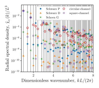
Figure 2: Semi-log plot of the radial spectral densities $\tilde{\chi}_{{}_{V}}(k)$ as functions of the dimensionless wavenumber $kL/(2\pi)$ for the five triply periodic models with porosity $\phi_{1}=0.5$: Schwarz P, Schwarz D, Schoen G, circular-channel model, and square-channel model. Here, $L$ is the side length of the cubic simulation box. Due to the periodicity of these models, $\mathinner{\tilde{\chi}_{{}_{V}}\mathopen{\left(k\right)}}$ is nonzero only at the Bragg peaks of the simple cubic lattice (shown in gray vertical lines).

4.2 Local Volume-Fraction Variance

Substitution of Eq. (43) for the spectral density into Eq. (16) yields an explicit expression for the local volume-fraction variance $\sigma_{{}_{V}}^{2}(R)$ for the triply periodic media models considered here:

$$\sigma_{{}_{V}}^{2}(R) =\frac{1}{2\pi^{2}v_{1}(R)}\int_{0}^{\infty}k^{2}{\tilde{\chi}}_{{}_{V}}(k){\tilde{\alpha}}_{2}(k;R)\differential{k}$$

$$=\frac{1}{2v_{1}(R)L^{3}}\sum_{n=1}^{\infty}Z(Q_{n})\tilde{A}_{2}(Q_{n};\Omega){\tilde{\alpha}}_{2}(Q_{n};R)$$

$$=\frac{3\pi^{2}}{v_{1}(R)L^{3}}\sum_{n=1}^{\infty}Z(Q_{n})\tilde{A}_{2}(Q_{n};\Omega)\frac{J^{2}_{3/2}(Q_{n}R)}{{Q_{n}}^{3}}.$$ (47)

where we have used the angular-averaged formula (44) for the spectral density. Substitution of Eq. (44) into Eq. (23) yields the corresponding expression for the large-$R$ asymptotic coefficient [46]:

$$\overline{B}_{V}=\frac{9}{4}\sum_{n=1}^{\infty}Z(Q_{n})\frac{\tilde{A}_{2}(Q_{n};\Omega)}{L^{3}(Q_{n}L)^{4}}.$$ (48)

We compute the local volume-fraction variance $\sigma_{{}_{V}}^{2}(R)$ as a function of window radius $R$ for the five triply periodic structures with $\phi_{1}=1/2$ from Eq. (47). Since these five structures are periodic and, hence, class I hyperuniform, their variances decay as fast as $R^{-4}$ for large radii ($R\gg L$). In Fig. 3, we plot the variances on a log-log scale for the three triply periodic minimal surfaces: Schwarz P, Schwarz D, and Schoen G. The results for the square- and circular-channel models are not shown, since they are virtually indistinguishable from that of the Schwarz P on the scale of this figure. The values of the large-$R$ asymptotic coefficient $\overline{B}_{V}$ for the five triply periodic structures, as computed from Eq. (48) and listed in Table 2, enable us to rank order the structures according to their large-scale volume-fraction fluctuations. Table 2 also includes the result for a spherical obstacle at the centroid of the cubic cell (spherical-obstacle model) at $\phi_{1}=1/2$. We see that the Schwarz P structure has the largest large-scale volume-fraction fluctuations, followed by the circular-channel model, the square-channel model, the spherical-obstacle model, the Schoen G structure, and finally, the Schwarz D structure has the smallest value of $\overline{B}_{V}$. Importantly, we will see in Sec. 5.2 that these rankings of the structures are wholly consistent with the rankings of their fluid permeabilities.

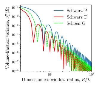
Figure 3: Log-log plot of the local volume-fraction variance $\sigma_{{}_{V}}^{2}(R)$ as a function of the dimensionless window radius $R/L$ for the three triply periodic minimal surfaces with porosity $\phi=0.5$: Schwarz P, Schwarz D, and Schoen G. For large radii ($R/L\gg 1$), the variance $\sigma_{{}_{V}}^{2}(R)$ of all models commonly decays as fast as $R^{-4}$. On average, the Schwarz P and D structures have the largest and smallest variances, respectively.

Table 2: Hyperuniformity order metric $\overline{B}_{V}$ for six triply periodic models with porosity $\phi=1/2$: Schwarz P, Schwarz D, Schoen G, circular-channel model, square-channel model, and spherical-obstacle model. The models are arranged in an ascending order of $\overline{B}_{V}$. The quantities are computed by taking the side length of the cubic fundamental cell to be unity, i.e., $L=1$.

Model	$\overline{B}_{V}$
Schwarz P	$4.936\times 10^{-4}$
circular-channel	$4.721\times 10^{-4}$
square-channel	$4.504\times 10^{-4}$
spherical obstacle	$4.462\times 10^{-4}$
Schoen G	$1.376\times 10^{-4}$
Schwarz D	$6.002\times 10^{-5}$

4.3 Pore-Size Functions

To compute rigorous bounds on the mean survival time, Gevertz and Torquato [14] obtained accurate quintic polynomial fits of pore-size density function $P(\delta)$ for four triply periodic models: the circular-channel model, and Schwarz P, Schoen G, and Schwarz D structures. Here, we improve these polynomial expressions for $P(\delta)$ by imposing the exact constraint at the origin, i.e., $P(0)=s/\phi_{1}$, from independent direct numerical simulations of the pore-size density function. Furthermore, via an additional simulation, we obtain an accurate polynomial fit of $P(\delta)$ for the square-channel model, which exactly dictates a cubic polynomial for this model. To summarize, we find the following accurate fits of $P(x)$ for all five triply periodic bicontinuous models, where $x\equiv\delta/L$:

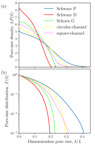
Figure 4: Plots of (a) the dimensionless pore-size probability density function $LP(\delta)$ and (b) the corresponding complementary cumulative distribution function $F(\delta)$ as functions of dimensionless pore radius $\delta/L$ for the five triply periodic models with porosity $\phi_{1}=0.5$: Schwarz P, Schwarz D, Schoen G, circular-channel model, and square-channel model. Here, $L$ is the side length of the cubic periodic simulation box. The curves, which are in very good agreement with direct simulations, are generated from the polynomial fits (49)-(53).

Table 3: The dimensionless first moment $\langle\delta\rangle/L$ (mean pore size) and second moment $\langle\delta^{2}\rangle/L^{2}$ of the pore-size density function $P(\delta)$ for the five triply periodic models at porosity $\phi_{1}=0.5$, as obtained from the polynomial fits given in Eqs. (49)-(53), which are in excellent agreement with direct simulations of these moments. We also list the corresponding values of the inverse of the dimensionless specific surface $(sL)^{-1}$ taken from Ref. [13]. Models are arranged in an ascending order of $\langle\delta^{2}\rangle/L^{2}$ from bottom to top. Note that the same ordering applies to the mean pore size $\langle\delta\rangle/L$ and $(sL)^{-1}$. Here, $L$ is the side length of the cubic unit cell.

Model	$\langle\delta\rangle/L$	$\langle\delta^{2}\rangle/L^{2}$	$(sL)^{-1}$
Schwarz P	1.222(8)$\times 10^{-1}$	2.218(1)$\times 10^{-2}$	$4.219\times 10^{-1}$
circular-channel	1.080(7)$\times 10^{-1}$	1.681(3)$\times 10^{-2}$	$3.788\times 10^{-1}$
square-channel	9.726(1)$\times 10^{-2}$	1.379(4)$\times 10^{-2}$	$3.333\times 10^{-1}$
Schoen G	8.812(1)$\times 10^{-2}$	1.104(1)$\times 10^{-2}$	$3.197\times 10^{-1}$
Schwarz D	7.104(5)$\times 10^{-2}$	7.274(4)$\times 10^{-3}$	$2.563\times 10^{-1}$

$$\text{Schwarz P:}~{}P(x)$$

$$=\begin{cases}\parbox{121.41306pt}{$-3443x^{5}+3807.4x^{4}-1336.66x^{3}$ \\ $~{}~{}~{}+149.273x^{2}-13.7109x+5.02661$,}&x<0.441,\\ 0,&\text{otherwise},\end{cases}$$ (49)

$$\text{Schwarz D:}~{}P(x)$$

$$=\begin{cases}\parbox{121.41306pt}{ $9760x^{5}+8302.1x^{4}-4002.49x^{3}$ \\ $~{}~{}~{}+347.050x^{2}-32.1064x+8.31791$, }&x<0.230\\ 0,&\text{otherwise},\end{cases}$$ (50)

$$\text{Schoen G:}~{}P(x)$$

$$=\begin{cases}\parbox{121.41306pt}{ $55486x^{5}-33537.6x^{4}+6997.17x^{3}$ \\ $~{}~{}~{}-691.054x^{2}+15.2274x+6.25259$,}&x<0.238\\ 0,&\text{otherwise},\end{cases}$$ (51)

$$\text{circular-channel:}~{}P(x)$$

$$=\begin{cases}\parbox{121.41306pt}{ $2935x^{5}-813.9x^{4}-214.01x^{3}$\\ $~{}~{}~{}+37.925x^{2}-11.7534x+5.49471,$}&x<0.355\\ 0,&\text{otherwise},\end{cases}$$ (52)

$$\text{square-channel:}~{}P(x)$$

$$=\begin{cases}-66.9x^{2}-5.98x+6.021,&x<0.25\\ -534x^{3}+548.2x^{2}-188.66x+21.775,&0.25<x<0.352\\ 0,&\text{otherwise},\end{cases}$$ (53)

Figure 4 depicts the dimensionless pore-size probability density function $LP(\delta)$ and the corresponding complementary cumulative distribution function $F(\delta)$ as functions of dimensionless pore radius $\delta/L$ for the five triply periodic models with $\phi=1/2$, as computed from the polynomial fits (49)-(53). As expected, both functions for each model monotonically decrease with $\delta/L$ within a compactly supported interval, i.e., the functions are non-zero up to a finite and positive value of $\delta/L$. The Schwarz P structure has the largest such support among all structures, since it is capable of accommodating the largest spherical region at the centroid. By contrast, the Schwarz D structure has the smallest support among all structures, since it is characterized by narrow channels that cannot support a large pore, as can be inferred visually from the corresponding image shown in Fig. 1. The support sizes of the circular-channel and square-channel models are similar and lie between those of the Schwarz P and Schoen G structures.

The values of the dimensionless mean pore size or first moment $\langle\delta\rangle/L$ and second moment $\langle\delta^{2}\rangle/L^{2}$ of the five models computed from the fit functions are listed in Table 3. These estimates are in excellent agreement with corresponding simulation results with relative errors no larger than one percent. The table also includes the corresponding values of the inverse of the dimensionless specific surface $(sL)^{-1}$ taken from Ref. [13]. The relative rankings of the structures according to both the mean pore size and second moment as well as the inverse of the specific surface are the same: the values of the three quantities are largest for the Schwarz P structure, followed by the circular-channel model, square-channel model, Schoen G structure, and Schwarz D structure, which has the smallest ones.

5 Microstructure-Dependent Estimates of Transport Properties

5.1 Diffusion Spreadability

For the models of periodic media considered in this paper, we can obtain an explicit formula for the diffusion spreadability by substituting relation (43) for the spectral density into the general expression (38) for the spreadability (with $\phi_{1}=1/2$) to yield

$$\mathcal{S}(\infty)-\mathcal{S}(t)= \frac{1}{\pi^{2}}\int_{0}^{\infty}k^{2}\tilde{\chi}_{{}_{V}}(k)\exp(-k^{2}{\cal D}t)\differential{k}$$

$$= \frac{1}{L^{3}}\sum_{n=1}^{\infty}Z(Q_{n})\tilde{A}_{2}(Q_{n};\Omega)\exp(-{Q_{n}}^{2}\mathcal{D}t),$$ (54)

where we have used the angular-averaged formula (44) for the spectral density with $\tilde{A}_{2}(Q_{n};\Omega)$ given by (45). For the same reasons noted in Ref. [64], the first term in the sum of Eq. (54) is the dominant contribution at long times $(\mathcal{D}t/L^{2}\gg 1)$ and so all decay with the same exponential rate given by

$$\mathcal{S}(\infty)-\mathcal{S}(t)\sim C_{\cal S}(\Omega)\exp(-(2\pi)^{2}\mathcal{D}t/L^{2})\quad(\mathcal{D}t/L^{2}\gg 1),$$ (55)

where $C_{\cal S}(\Omega)$ is a structure-dependent constant given by

$$C_{\cal S}(\Omega)=\frac{6\tilde{A}_{2}(2\pi/L;\Omega)}{L^{3}},$$ (56)

and we have used the fact that the first Bragg peak is $Q_{1}=2\pi/L$ and $Z(Q_{1})=6$ for the simple cubic lattice.

Figure 5 shows the excess spreadability $\mathcal{S}(\infty)-\mathcal{S}(t)$ as a function of the dimensionless time $\mathcal{D}t/L^{2}$, as obtained from Eq. (54), for the Schwarz P, Schwarz D, and Schoen G structures. The corresponding curves for the circular- and square-channel models are indistinguishable from Schwarz P on the scale of this plot and so are not shown. We find that for a specific time, the excess spreadability is the largest for the Schwarz P structure, followed by the circular-channel model, square-channel models, Schoen G, and finally, the Schwarz D has the smallest excess spreadability. Importantly, these rankings are consistent with those of the fluid permeabilities, as shown below, as well as other structural descriptors, as described in Sec. 7. It is noteworthy that the asymptotic formula (55) is virtually identical to the exact relation (54) (relative errors within the $10^{-7}$ percent) for $\mathcal{D}t/L^{2}>1$, which is consistent with the values of the asymptotic coefficient $C_{\cal S}$ listed in Table. 4.

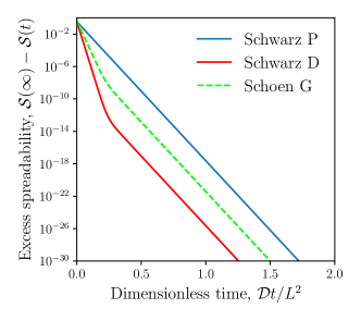
Figure 5: Semi-log plot of the excess spreadability $\mathcal{S}(\infty)-\mathcal{S}(t)$ as a function of dimensionless time $\mathcal{D}t/L^{2}$ for the three triply periodic minimal surfaces with porosity $\phi_{1}=1/2$: Schwarz P, Schwarz D, and Schoen G. The Schwarz P and D structures have the largest and smallest excess spreadabilities $\mathcal{S}(\infty)-\mathcal{S}(t)$, respectively. Curves for the circular- and square-channel models are not shown here because they are only slightly lower than but virtually identical to Schwarz P on the scale of this figure.

Table 4: The long-time asymptotic coefficient $C_{\cal S}$ of the excess spreadability $\mathcal{S}(\infty)-\mathcal{S}(t)$, defined by Eq. 56, for the five triply periodic structures with porosity $\phi_{1}=1/2$ studied in this paper.

Models	Coefficient $C_{\mathcal{S}}$
Schwarz P	$3.346\times 10^{-1}$
circular-channel	$3.191\times 10^{-1}$
square-channel	$3.039\times 10^{-1}$
Schoen G	$5.113\times 10^{-5}$
Schwarz D	$3.220\times 10^{-9}$

5.2 Fluid Permeability

Here we estimate the fluid permeabilities of each of the five triply periodic bicontinuous models using the approximation formula (33) and two-point void upper bound (35). Note that the formation factor in Eq. (33) for the triply periodic minimal surfaces is exactly given

$${\cal F}=3,$$ (57)

where we have used the exact expression (30) with $\sigma_{2}=0$. Moreover, this relation is an excellent approximation for the two pore-channel models, since $\zeta_{2}$ will be very insensitive to the small differences in geometries from the Schwarz P structure and much more sensitive to their topological similarities. To compute $\mathbbm{k}$ from Eq. (33), in addition to utilizing ${\cal F}=3$, we employ the second moments $\langle{\delta^{2}}\rangle$ given in Table 3.

Table 5: Estimates of the dimensionless fluid permeability $\mathbbm{k}/L^{2}$ for the five triply periodic models at porosity $\phi_{1}=1/2$ considered in this paper. For each model, the values are estimated via the direct simulations in Ref. [13], the formula (33), and two-point void bound (59). In each column, the value in the square brackets represents the ratio of the estimates of the corresponding model to that of Schwarz P. Models are arranged in ascending order of $\mathbbm{k}/L^{2}$ from the bottom to the top. Here, $L$ is the side length of the cubic fundamental cell.

Model	Direct simulation		Approximation: (33)		Two-point bound: Eq. (59)
Schwarz P	$3.4765\times 10^{-3}$	[ $1.000$ ]	$7.4211\times 10^{-3}$	[ $1.000$ ]	$1.2197\times 10^{-2}$	[ $1.000$ ]
circular-channel	$3.4596\times 10^{-3}$	[ $0.995$ ]	$5.5957\times 10^{-3}$	[ $0.754$ ]	$1.1741\times 10^{-2}$	[ $0.963$ ]
square-channel	$3.0744\times 10^{-3}$	[ $0.884$ ]	$4.6051\times 10^{-3}$	[ $0.621$ ]	$1.1258\times 10^{-2}$	[ $0.923$ ]
Schoen G	$2.2889\times 10^{-3}$	[ $0.658$ ]	$3.6824\times 10^{-3}$	[ $0.496$ ]	$6.5874\times 10^{-3}$	[ $0.540$ ]
Schwarz D	$1.4397\times 10^{-3}$	[ $0.414$ ]	$2.4244\times 10^{-3}$	[ $0.327$ ]	$4.3327\times 10^{-3}$	[ $0.355$ ]

The length scale $\ell_{P}$ involved in the two-point void upper bound (35) on $\mathbbm{k}$ can be expressed explicitly for these models by substituting Eq. (44) into Eq. (37)

$$\ell_{P}^{2}= \frac{1}{2L^{3}}\sum_{n=1}^{\infty}Z(Q_{n})\frac{\tilde{A}_{2}(Q_{n};\Omega)}{{Q_{n}}^{2}},$$ (58)

and, thus, the upper bound on the permeability can be expressed as

$$\mathbbm{k}\leq \frac{1}{3{\phi_{2}}^{2}L^{3}}\sum_{n=1}^{\infty}Z(Q_{n})\frac{\tilde{A}_{2}(Q_{n};\Omega)}{{Q_{n}}^{2}}.$$ (59)

In Table 5, we compare the estimates of the dimensionless fluid permeability $\mathbbm{k}/L^{2}$ from two microstructure-dependent formulas as obtained from Eqs. (33) and (59) to direct simulations via the immersed-boundary finite-volume method [13]. The formula (33) yields estimates that are within about a factor of two of the simulation results, which is actually relatively accurate for a permeability approximation that can applied to a broad range of structures; see Refs. [74] and [1] and references therein. While the void upper bound is not sharp, it provides the correct rankings of the structures according to their permeabilities, as does the approximation (33). The numbers indicated within the square brackets in each column of the table represent the values of $\mathbbm{k}/L^{2}$ scaled by that of Schwarz P estimated by the associated method. Note that all three scaled estimates yield identical relative rankings of $\mathbbm{k}/L^{2}$ for the five models: Schwarz P has the largest value, followed by the circular-channel model, the square-channel model, Schoen G, and finally, the Schwarz D has the lowest value. Thus, the estimate (33) and (59) can be employed to estimate $\mathbbm{k}/L^{2}$ given the corresponding reference value for the Schwarz P structure. These rankings of $\mathbbm{k}/L^{2}$ are consistent with the rankings of $\left\langle\delta^{2}\right\rangle$, demonstrating that the structures that have larger pores on average tend to have higher permeabilities.

6 Generalized Maximum-Permeability Conjecture for All Porosities

The maximum-permeability conjecture (see Conjecture 1 of the Introduction) applies to the special porosity value of $1/2$. Here we propose the following generalization of Conjecture 1 that applies for all nontrivial porosities, i.e., $0<\phi_{1}<1$:

Conjecture 2

Among three-dimensional porous media at some porosity $\phi_{1}\in(0,1)$ within a simple cubic fundamental cell of side length $L$ under periodic boundary conditions, the dimensionless isotropic fluid permeability $\mathbbm{k}/L^{2}$ is maximized for the medium in which the pore space is simply connected with an interface that minimizes the total interface area.

This conjecture is based on the fact that simply connected pore spaces with smaller total interfacial areas should offer less resistance to Stokes flow (due to the non-slip boundary condition) and, hence, larger fluid permeabilities. Here we provide rigorous theoretical arguments that support Conjecture 2 at the two extreme limits of the porosity, i.e., $\phi_{1}\to 0$ and $\phi_{1}\to 1$. First, we describe what geometries, at these two limits, minimize the total surface area $\cal A$ within a cubic box of side length $L$, i.e., minimizes the specific surface $s={\cal A}/L^{3}$, without regard to fluid transport. It is well-known that simple, single convex shapes minimize $\cal A$, depending on the fraction of space occupied by these domains; they are the sphere, the circular cylinder aligned with a cube edge and the square slab whose planar interfaces are parallel to a cube face [75]. Among these three geometries, the sphere has the smallest specific surface in the volume-fraction interval $[0,4\pi/81\approx 0.1551)$, the cylinder has the smallest specific surface in the volume-fraction interval $[4\pi/81,\pi^{-1}\approx 0.3183)$, and the square slab has the smallest specific surface for $\phi>\pi^{-1}$.

Now consider the geometry that maximizes the fluid permeability in the low-porosity limit, i.e., $\phi_{1}\to 0$. In this case, it is clear that the pore space must be simply and topologically connected in all three principal directions. This condition eliminates a very small fluid-filled sphere, which has a zero permeability. Thus, given that a cylinder has the smallest specific surface among all simply connected pore regions at low porosities, it is natural to consider a pore space consisting of circular cylinders that leads to an isotropic fluid permeability, namely, the circular-channel model consisting of three such tubes that are aligned along the principal axes and that intersect at the centroid of the cubic cell. The exact solution for such a geometry can easily be obtained from the well-known solution for a single circular cylindrical tube of radius $a$ and length $L$ that passes through the centroid of the fundamental cell and aligned with a cube edge [27, 1], which is given by

$$\mathbbm{k}=\frac{a^{2}}{8}\phi$$ (60)

and is  known to maximize the fluid permeability in a single direction. Given that $\phi=\pi(a/L)^{2}$, we can rewrite Eq. (60) in terms of the length scale $L$:

$$\mathbbm{k}=\frac{L^{2}}{8\pi}\phi^{2}.$$ (61)

From this solution and the fact that total porosity of the circular-channel model is $\phi_{1}=3\phi$ in the limit $\phi_{1}\to 0$, we arrive at the exact expression for the aforementioned three intersecting cylindrical tubes (see the leftmost structure in the top row of Fig. 6) that maximizes the isotropic fluid permeability in the low-porosity limit:

$$\mathbbm{k}\approx\frac{L^{2}}{72\pi}\phi_{1}^{2}\qquad(\phi_{1}\to 0).$$ (62)

Next, consider the geometry that maximizes the fluid permeability in the high-porosity limit, i.e., $\phi_{1}\to 1$. In this limit, the geometry must involve Stokes flow around a single solid body, which must be spherical in order to achieve an isotropic permeability (see rightmost structure in the top row of Fig. 6). It is well-known that such a body minimizes the drag force [76] or, equivalently, maximizes the permeability, which is inversely related to the drag force [1], which in the dilute-particle-concentration limit is given by

$$\mathbbm{k}= \frac{2a^{2}}{9(1-\phi_{1})}\qquad(\phi_{1}\to 1),$$ (63)

where we have used that $1-\phi_{1}=4\pi(a/L)^{3}/3$ to obtain the last line. Given that $1-\phi_{1}=4\pi(a/L)^{3}/3$, we can rewrite this expression in terms of the length scale $L$:

$$\mathbbm{k}=\frac{L^{2}}{18(1-\phi_{1})^{1/3}}\left(\frac{6}{\pi}\right)^{2/3}\qquad(\phi_{1}\to 1).$$ (64)

As shown above, a sphere at low porosities has the smallest specific surface measure with respect to the cube side length $L$. This is consistent with the fact that a spherical obstacle maximizes the isotropic fluid permeability $\mathbbm{k}$ in the limit $\phi_{1}\to 1$.

For porosities intermediate between 0 and $1/2$, where the optimal structure is conjectured to be the Schwarz P medium [13] (middle image in the top row of Fig. 6), the maximum-permeability structures must still be bicontinuous with a pore space that is topologically equivalent (i.e., homeomorphic) to that of the Schwarz P structure, i.e., orthogonally oriented cylinder-like channels that intersect at the centroid of the cube. As $\phi_{1}$ gradually increases from $0$ to $1/2$, the infinite curvature at the cylinder junctures must become finite, leading to increasingly smoother juncture regions in cylinder-like channel geometries as $\phi_{1}$ increases until the very smooth Schwarz P minimal surface is reached at $\phi_{1}=1/2$. The leftmost image in the bottom row of Fig. 6 schematically shows such an optimal structure with a porosity that lies in between 0 and $1/2$ and that putatively has a minimal interfacial area. As $\phi_{1}$ gradually increases beyond $\phi_{1}=1/2$, the Schwarz P surface deforms continuously (with a concomitant increase in the cross-sectional area of cylinder-like channels) such that the connected solid phase eventually has a “pinch-off” porosity point where the solid phase becomes disconnected until $\phi_{1}$ approaches unity when it becomes an isolated sphere. The rightmost image in the bottom row of Fig. 6 schematically shows such an optimal structure with a porosity that lies in between $1/2$ and $1$ and that putatively has a minimal interfacial area. We note that a family of surfaces possessing the symmetry and topology of the Schwarz P surface but with different porosities were presented in Ref. [18], but these structures were not shown to possess minimal specific surfaces.

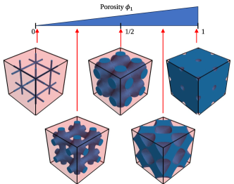
Figure 6: The top row of configurations shows the conjectured Schwarz P structure that maximizes the fluid permeability $\mathbbm{k}/L^{2}$ as well as the triply periodic models that we have shown maximize $\mathbbm{k}/L^{2}$ in the limit $\phi_{1}\to 0$ (circular-channel model) and limit $\phi_{1}\to 1$ (spherical obstacle). The bottom row of images, from left to right, show schematics of the triply periodic structures that are expected to maximize the fluid permeability at porosities that lies in between 0 and $1/2$ and in between 1/2 and $1$, respectively. The solid phase here is no longer connected and remains disconnected until $\phi_{1}$ approaches unity when it becomes a sphere. In all cases, $2\times 2\times 2$ fundamentals cells are presented, where opaque blue and transparent red depict the domains of the porous phase and solid phase, respectively.

7 Discussion

We have determined various microstructural characteristics, including the spectral densities, pore-size distribution functions, local volume-fraction variances and hyperuniformity order metrics of the five triply periodic bicontinuous media models shown in Fig. 1: Schwarz P, Schwarz D, and Schoen G minimal structures as well as the circular-channel and square-channel models. We also computed the formation factor $\cal F$ and combined this information with the second moment of the pore-size function to estimate, for the first time, the fluid permeability $\mathbbm{k}$ for all five models via the explicit microstructure-dependent formula (33). These predictions are shown to be in relatively good agreement with direct computer simulations of the permeabilities [13]. While the void bound (35), which we also computed via the spectral density, lay appreciably above the simulation data, it provides the same trends in the relative rankings of the five models in which, consistent with Conjecture 1, identifies the Schwarz P structure with the highest permeability. We also calculated the time-dependent diffusion spreadability ${\cal S}(t)$ as a function of time $t$ for all five models, which again shows the same trends as for $\mathbbm{k}$.

Table 6: Summary of the key structural and physical properties for the five triply periodic structures with porosity $\phi_{1}=1/2$ studied in in this paper: inverse of the dimensionless specific surface $(sL)^{-1}$ (taken from Ref. [13]), hyperuniformity order metric $\overline{B}_{V}$ (Table 2), the dimensionless pose-size second moment $\langle\delta^{2}\rangle/L^{2}$ (Table 3), dimensionless fluid permeability $\mathbbm{k}/L^{2}$ (the second column of Table 5), and the long-time asymptotic coefficient $C_{\mathcal{S}}$ of the excess spreadability $\mathcal{S}(\infty)-\mathcal{S}(t)$ [see Eq. (55)]. Here, $L$ is the side length of the cubic fundamental cell.

Quantity	Schwarz P	circular-channel	square-channel	Schoen G	Schwarz D
$(sL)^{-1}$	$4.219\times 10^{-1}$	$3.788\times 10^{-1}$	$3.333\times 10^{-1}$	$3.197\times 10^{-1}$	$2.563\times 10^{-1}$
$\overline{B}_{V}$	$4.936\times 10^{-4}$	$4.721\times 10^{-4}$	$4.504\times 10^{-4}$	$1.376\times 10^{-4}$	$6.002\times 10^{-5}$
$\langle\delta^{2}\rangle/L^{2}$	2.218$\times 10^{-2}$	1.681$\times 10^{-2}$	1.379$\times 10^{-2}$	1.104$\times 10^{-2}$	7.274$\times 10^{-3}$
$\mathbbm{k}/L^{2}$	$3.4765\times 10^{-3}$	$3.4596\times 10^{-3}$	$3.0744\times 10^{-3}$	$2.2889\times 10^{-3}$	$1.4397\times 10^{-3}$
$C_{\mathcal{S}}$	$3.346\times 10^{-1}$	$3.191\times 10^{-1}$	$3.039\times 10^{-1}$	$5.113\times 10^{-5}$	$3.220\times 10^{-9}$

It is noteworthy that the dimensionless permeability $\mathbbm{k}/L^{2}$ for the five models is not only positively correlated with inverse of the dimensionless specific surface $(sL)^{-1}$, as shown in Ref. [13], but also, as shown here, with the hyperuniformity order metric $\overline{B}_{V}$ (see Table 2), the dimensionless pore-size second moment $\langle{\delta^{2}}\rangle/L^{2}$ (see Table 3), and the long-time asymptotic coefficient $C_{\mathcal{S}}$ of excess spreadability $\mathcal{S}(\infty)-\mathcal{S}(t)$ [see Eq. (55)]; see the specific values summarized in Table 6. It can be seen that the relative rankings of the five models according to all of these characteristics are the same, namely, in descending order the Schwarz P structures possess the largest values, followed by the circular-channel model, the square-channel model, the Schoen G, and the Schwarz D, the latter having the smallest values. Structures with a smaller dimensionless specific surface [i.e., larger $(sL)^{-1}$] tend to possess domains of solid and void phases that are distributed less uniformly throughout the fundamental cell, leading to larger values $\overline{B}_{V}$. The positive correlation between $\langle\delta^{2}\rangle/L^{2}$ and $\mathbbm{k}/L^{2}$ is consistent with the fact that a larger effective pore-channel area in a principal direction, measured by $\pi\langle\delta^{2}\rangle/L^{2}$, facilitates fluid transport, given the same formation factor. Similarly, the positive correlation between the coefficient $C_{\mathcal{S}}$  and $\mathbbm{k}/L^{2}$ is consistent with the fact that structures with larger pore regions, as measured by the dimensionless second moment $\langle\delta^{2}\rangle/L^{2}$, means that it takes longer for solute species to diffuse and fill the entire pore space. Thus, this latter correlation establishes yet another cross-property relation between the fluid permeability and diffusion properties for these triply periodic media but, in this case, a time-dependent transport property. It was previously established that the steady-state mean survival time $\tau$ rank orders the five triply periodic media models in exactly the same way as $\mathbbm{k}$ [14].

An outstanding problem for future research is the determination of the triply periodic bicontinuous media within a cubic fundamental cell of side length $L$ with minimal dimensionless specific surface $sL$ for arbitrary porosities subject to cubic symmetry. This would be the first step in validating Conjecture 2. Its full validation would require one to show that such optimal structures with minimal $sL$ also maximize the isotropic fluid permeability under the aforementioned constraints.

Appendix A Phase-Inversion Symmetry of Triply Periodic Minimal Surfaces

Here, we prove that three triply periodic minimal surfaces (Schwarz P, Schwarz D, and Schoen G) with porosity $\phi=1/2$ possess phase-inversion symmetry [1], i.e., the $n$-point correlation functions, defined in Sec. 2.1, obey the following symmetry conditions:

$$S_{n}^{(1)}({\bf x}_{1},...,{\bf x}_{n})=S_{n}^{(2)}({\bf x}_{1},...,{\bf x}_{n})\quad(n=2,3,\ldots).$$ (65)

It is straightforward to prove Eq. (65) for the Schwarz P and D structures by using the definition of $S_{n}^{(i)}$, since, for each model, the solid-phase and void-phase domains are identical under simple translations:

$$\text{Schwarz P}:\quad {\cal I}^{(1)}({\bf r})={\cal I}^{(2)}({\bf r}+L/2(\hat{\bf x}+\hat{\bf y}+\hat{\bf z})),$$ (66)

$$\text{Schwarz D}:\quad {\cal I}^{(1)}({\bf r})={\cal I}^{(2)}({\bf r}+L/2\hat{\bf x}),$$ (67)

where $\hat{\bf x}$, $\hat{\bf y}$, and $\hat{\bf z}$ are unit vectors in the directions of $x$, $y$, and $z$ axes, respectively. For Schoen G, one can prove Eq. (65) by using the fact that its solid- and void-phase domains are identical under a point reflection, i.e.,

$$\text{Schoen G}:\quad {\cal I}^{(1)}({\bf r})={\cal I}^{(2)}(-{\bf r}+L/2\hat{\bf y}).$$ (68)

Applying Eq. (68) to the definition of $S_{n}^{(i)}$, we now prove Eq. (65) for Schoen G structure:

$$S_{n}^{(1)}({\bf x}_{1},\ldots,{\bf x}_{n})\equiv\left\langle\prod_{i=1}^{n}{\cal I}^{(1)}({\bf x}_{i})\right\rangle=\left\langle\prod_{i=1}^{n}{\cal I}^{(2)}(-{\bf x}_{i}+L/2\hat{\bf y})\right\rangle$$

$$= S_{n}^{(2)}(-{\bf x}_{1}+L/2\hat{\bf y},-{\bf x}_{2}+L/2\hat{\bf y},\ldots,-{\bf x}_{n}+L/2\hat{\bf y})$$

$$= S_{n}^{(2)}(-{\bf x}_{1},-{\bf x}_{2},\ldots,-{\bf x}_{n})=S_{n}^{(2)}({\bf x}_{1},{\bf x}_{2},\ldots,{\bf x}_{n})\quad\mathrm{for~{}}n\geq 2,$$ (69)

the last line of which implies statistically homogeneity.

References

- [1] S. Torquato, Random Heterogeneous Materials: Microstructure and Macroscopic Properties, Springer-Verlag, New York, 2002.
- [2] G. W. Milton, The Theory of Composites, Cambridge University Press, Cambridge, England, 2002.
- [3] M. Sahimi, Heterogeneous Materials I: Linear Transport and Optical Properties, Springer-Verlag, New York, 2003.
- [4] T. Zohdi, P. Wiggers, Introduction to Computational Micromechanics, Springer-Verlag, New York, 2005.
- [5] Z. Hashin, S. Shtrikman, A variational approach to the theory of the effective magnetic permeability of multiphase materials, J. Appl. Phys. 33 (1962) 3125–3131. doi:10.1063/1.1728579.
- [6] K. A. Lurie, A. V. Cherkaev, The problem of formation of an optimal multicomponent composite, J. Opt. Theor. Appl. 46 (1985) 571–580. doi:10.1007/bf01238903.
- [7] G. W. Milton, Modelling the properties of composites by laminates, in: J. L. Eriksen, et al. (Eds.), Homogenization and Effective Moduli of Materials and Media, Springer-Verlag, New York, 1986.
- [8] S. B. Vigdergauz, Regular structures with extremal elastic properties, Mech. Solids 24 (1989) 57–63.
- [9] M. Vaezi, H. Seitz, S. Yang, A review on 3d micro-additive manufacturing technologies, The International Journal of Advanced Manufacturing Technology 67 (2013) 1721–1754.
- [10] S. Torquato, S. Hyun, A. Donev, Multifunctional composites: Optimizing microstructures for simultaneous transport of heat and electricity, Phys. Rev. Lett. 89 (2002) 266601. doi:10.1103/PhysRevLett.89.266601.
- [11] S. Torquato, S. Hyun, A. Donev, Optimal design of manufacturable three-dimensional composites with multifuctional characteristics, J. Appl. Phys. 94 (2003) 5748–5755. doi:10.1063/1.1611631.
- [12] S. Torquato, A. Donev, Minimal surfaces and multifunctionality, Proc. R. Soc. Lond. A 460 (2004) 1849–1856. doi:10.1103/PhysRevE.72.056319.
- [13] Y. Jung, S. Torquato, Fluid permeabilities of triply periodic minimal surfaces, Phys. Rev. E 92 (2005) 255505. doi:10.1103/PhysRevE.72.056319.
- [14] J. L. Gevertz, S. Torquato, Mean survival times of absorbing triply periodic minimal surfaces, Phys. Rev. E 80 (2009) 011102. doi:10.1103/PhysRevE.80.011102.
- [15] D. M. Anderson, H. T. Davis, L. E. Scriven, J. C. C. Nitsche, Periodic surfaces of prescribed mean curvature, in: Advances in Chemical Physics, John Wiley & Sons, Ltd, 1990, pp. 337–396. doi:10.1002/9780470141267.ch6.
- [16] A. L. Mackay, Crystallographic surfaces, Proc. R. Soc. Lond. 442 (1914) (1997) 47–59. doi:10.1098/rspa.1993.0089.
- [17] J. Klinowski, A. L. Mackay, H. Terrones, Curved surfaces in chemical structure, Philos. Trans. R. Soc. Lond. 354 (1715) (1997) 1975–1987. doi:10.1098/rsta.1996.0086.
- [18] R. Jullien, J.-F. Sadoc, R. Mosseri, Packing at random in curved space and frustration: A numerical study, J. Physique I 7 (1997) 1677–1692. doi:10.1051/jp1:1997162.
-
[19]
E. A. Lord, A. L. Mackay, Periodic
minimal surfaces of cubic symmetry, Curr. Sci. 85 (3) (2003) 346–362.
URL https://www.jstor.org/stable/24108665 - [20] P. D. Olmsted, S. T. Milner, Strong segregation theory of bicontinuous phases in block copolymers, Macromolecules 31 (12) (1998) 4011–4022. doi:10.1021/ma980043o.
- [21] Y. Lu, Y. Yang, A. Sellinger, M. Lu, J. Huang, H. Fan, R. Haddad, G. Lopez, A. R. Burns, D. Y. Sasaki, J. Shelnutt, C. J. Brinker, Self-assembly of mesoscopically ordered chromatic polydiacetylene/silica nanocomposites, Nature 410 (6831) (2001) 913–917. doi:10.1038/35073544.
- [22] P. Ziherl, R. D. Kamien, Soap froths and crystal structures, Phys. Rev. Lett. 85 (16) (2000) 3528–3531. doi:10.1103/PhysRevLett.85.3528.
- [23] S. C. Kapfer, S. T. Hyde, K. Mecke, C. H. Arns, G. E. Schröder-Turk, Minimal surface scaffold designs for tissue engineering, Biomaterials 32 (2011) 6875–6882. doi:10.1016/j.biomaterials.2011.06.012.
- [24] W. M. Gelbart, A. Ben-Shaul, D. Roux, Micelles, Membranes, Microemulsions, and Monolayers, Springer Science & Business Media, 2012.
- [25] T. Landh, From entangled membranes to eclectic morphologies: cubic membranes as subcellular space organizers, FEBS Lett. 369 (1) (1995) 13–17. doi:10.1016/0014-5793(95)00660-2.
- [26] National Research Council, and Solid State Sciences Committee, Biomolecular Self-Assembling Materials: Scientific and Technological Frontiers, National Academies Press, 1996.
- [27] A. E. Scheidegger, The Physics of Flow Through Porous Media, University of Toronto Press, Toronto, Canada, 1974.
- [28] S. Torquato, G. Stell, Microstructure of two-phase random media: I. The -point probability functions, J. Chem. Phys. 77 (1982) 2071–2077. doi:10.1063/1.444011.
- [29] D. Stoyan, W. S. Kendall, J. Mecke, Stochastic Geometry and Its Applications, 2nd Edition, Wiley, New York, 1995.
- [30] P. Debye, A. M. Bueche, Scattering by an inhomogeneous solid, J. Appl. Phys. 20 (1949) 518–525. doi:10.1063/1.1698419.
- [31] P. Debye, H. R. Anderson, H. Brumberger, Scattering by an inhomogeneous solid. II. The correlation function and its applications, J. Appl. Phys. 28 (1957) 679–683. doi:10.1063/1.1722830.
- [32] S. Torquato, Predicting transport characteristics of hyperuniform porous media via rigorous microstructure-property relations, Adv. Water Resour. 140 (2020) 103565. doi:10.1016/j.advwatres.2020.103565.
- [33] S. Torquato, F. H. Stillinger, Local density fluctuations, hyperuniform systems, and order metrics, Phys. Rev. E 68 (2003) 041113. doi:10.1103/PhysRevE.68.041113.
- [34] S. Torquato, Hyperuniform states of matter, Phys. Rep. 745 (2018) 1–95. doi:10.1016/j.physrep.2018.03.001.
- [35] Z. Ding, Y. Zheng, Y. Xu, Y. Jiao, W. Li, Hyperuniform flow fields resulting from hyperuniform configurations of circular disks, Phys. Rev. E 98 (2018) 063101. doi:10.1103/PhysRevE.98.063101.
- [36] C. E. Zachary, S. Torquato, Hyperuniformity in point patterns and two-phase heterogeneous media, J. Stat. Mech.: Theory & Exp. 2009 (2009) P12015. doi:10.1088/1742-5468/2009/12/P12015.
- [37] B. L. Lu, S. Torquato, Local volume fraction fluctuations in heterogeneous media, J. Chem. Phys. 93 (1990) 3452–3459. doi:10.1063/1.458827.
- [38] S. Torquato, F. H. Stillinger, New conjectural lower bounds on the optimal density of sphere packings, Exp. Math. 15 (2006) 307–331. doi:10.1080/10586458.2006.10128964.
- [39] J. Quintanilla, S. Torquato, Local volume fraction fluctuations in random media, J. Chem. Phys. 106 (1997) 2741–2751. doi:10.1063/1.473414.
- [40] S. Torquato, Disordered hyperuniform heterogeneous materials, J. Phys.: Cond. Mat 28 (2016) 414012. doi:10.1088/0953-8984/28/41/414012.
- [41] C. E. Zachary, S. Torquato, Anomalous local coordination, density fluctuations, and void statistics in disordered hyperuniform many-particle ground states, Phys. Rev. E 83 (2011) 051133. doi:10.1103/PhysRevE.83.051133.
- [42] M. Florescu, S. Torquato, P. J. Steinhardt, Designer disordered materials with large complete photonic band gaps, Proc. Nat. Acad. Sci. U. S. A. 106 (2009) 20658–20663. doi:10.1073/pnas.0907744106.
- [43] L. S. Froufe-Pérez, M. Engel, J. José Sáenz, F. Scheffold, Band gap formation and anderson localization in disordered photonic materials with structural correlations, Proc. Nat. Acad. Sci. 114 (2017) 9570–9574. doi:10.1073/pnas.1705130114.
- [44] S. Torquato, J. Kim, Nonlocal effective electromagnetic wave characteristics of composite media: Beyond the quasistatic regime, Phys. Rev. X 11 (2021) 021002. doi:10.1103/PhysRevX.11.021002.
- [45] O. Christogeorgos, H. Zhang, Q. Cheng, Y. Hao, Extraordinary Directive Emission and Scanning from an Array of Radiation Sources with Hyperuniform Disorder, Phys. Rev. Appl. 15 (2021) 014062. doi:10.1103/PhysRevApplied.15.014062.
- [46] J. Kim, S. Torquato, Characterizing the hyperuniformity of ordered and disordered two-phase media, Phys. Rev. E 103 (2021) 012123. doi:10.1103/PhysRevE.103.012123.
- [47] S. Torquato, Extraordinary disordered hyperuniform multifunctional composites, J. Composite Mater. 56 (23) (2022) 3635–3649. doi:10.1177/0021998322111643.
- [48] M. Merkel, M. Stappers, D. Ray, C. Denz, J. Imbrock, Stealthy hyperuniform surface structures for efficiency enhancement of organic solar cells, Adv. Photonics Res. 5 (2023) 2300256. doi:doi.org/10.1002/adpr.202300256.
- [49] S. Torquato, M. Skolnick, J. Kim, Local order metrics for two-phase media across length scales*, J. Phys. A: Math. & Theor. 55 (27) (2022) 274003. doi:10.1088/1751-8121/ac72d7.
- [50] S. Torquato, M. Avellaneda, Diffusion and reaction in heterogeneous media: Pore size distribution, relaxation times, and mean survival time, J. Chem. Phys. 95 (1991) 6477–6489. doi:10.1063/1.461519.
- [51] D. A. Coker, S. Torquato, J. H. Dunsmuir, Morphology and physical properties of Fontainebleau sandstone via a tomographic analysis, J. Geophys. Res. 101 (1996) 17497–17506. doi:10.1029/96JB00811.
- [52] S. Torquato, Effective electrical conductivity of two-phase disordered composite media, J. Appl. Phys. 58 (1985) 3790–3797. doi:10.1063/1.335593.
- [53] M. Avellaneda, S. Torquato, Rigorous link between fluid permeability, electrical conductivity, and relaxation times for transport in porous media, Phys. Fluids A 3 (1991) 2529–2540. doi:10.1063/1.858194.
- [54] D. L. Johnson, J. Koplik, L. M. Schwartz, New pore-size parameter characterizing transport in porous media, Phys. Rev. Lett. 57 (1986) 2564–2567. doi:10.1103/PhysRevLett.57.2564.
- [55] S. Torquato, Relationship between permeability and diffusion-controlled trapping constant of porous media, Phys. Rev. Lett. 64 (1990) 2644–2646. doi:10.1103/PhysRevLett.64.2644.
- [56] M. A. Klatt, R. M. Ziff, S. Torquato, Critical pore radius and transport properties of disordered hard-and overlapping-sphere models, Phys. Rev. E 104 (2021) 014127. doi:10.1103/PhysRevE.104.014127.
- [57] S. Prager, Viscous flow through porous media, Phys. Fluids 4 (1961) 1477–1482. doi:10.1063/1.1706246.
- [58] J. G. Berryman, G. W. Milton, Normalization constraint for variational bounds on fluid permeability, J. Chem. Phys. 83 (1985) 754–760. doi:10.1063/1.449489.
- [59] W. B. Russel, D. A. Saville, W. R. Schowalter, Colloidal Dispersions, Cambridge University Press, Cambridge, England, 1989.
- [60] J. Rubinstein, S. Torquato, Flow in random porous media: Mathematical formulation, variational principles, and rigorous bounds, J. Fluid Mech. 206 (1989) 25–46. doi:10.1017/S0022112089002211.
- [61] J. Kim, S. Torquato, New tessellation-based procedure to design perfectly hyperuniform disordered dispersions for materials discovery, Acta Materialia 168 (2019) 143–151. doi:10.1016/j.actamat.2019.01.026.
- [62] J. Kim, S. Torquato, Methodology to construct large realizations of perfectly hyperuniform disordered packings, Phys. Rev. E 99 (2019) 052141. doi:10.1103/PhysRevE.99.052141.
- [63] S. Torquato, D. C. Pham, Optimal bounds on the trapping constant and permeability of porous media, Phys. Rev. Lett. 92 (2004) 255505. doi:10.1103/PhysRevLett.92.255505.
- [64] S. Torquato, Diffusion spreadability as a probe of the microstructure of complex media across length scales, Phys. Rev. E 104 (2021) 054102. doi:10.1103/PhysRevE.104.054102.
- [65] P. P. Mitra, P. N. Sen, L. M. Schwartz, P. Le Doussal, Diffusion propagator as a probe of the structure of porous media, Phys. Rev. Lett. 68 (1992) 3555. doi:10.1103/PhysRevLett.68.3555.
- [66] D. S. Novikov, J. H. Jensen, J. A. Helpern, E. Fieremans, Revealing mesoscopic structural universality with diffusion, Proc. Nat. Acad. Sci. 111 (2014) 5088–5093. doi:10.1073/pnas.1316944111.
- [67] H. Wang, S. Torquato, Dynamic measure of hyperuniformity and nonhyperuniformity in heterogeneous media via the diffusion spreadability, Phys. Rev. Appl. 17 (2022) 034022. doi:10.1103/PhysRevApplied.17.034022.
- [68] M. Skolnick, S. Torquato, Simulated diffusion spreadability for characterizing the structure and transport properties of two-phase materials, Acta Materialia 250 (2023) 118857. doi:10.1016/j.actamat.2023.118857.
- [69] C. E. Maher, Y. Jiao, S. Torquato, Hyperuniformity of maximally random jammed packings of hyperspheres across spatial dimensions, Phys. Rev. E 108 (2023) 064602. doi:10.1103/PhysRevE.108.064602.
- [70] S. Torquato, Hyperuniformity and its generalizations, Phys. Rev. E 94 (2016) 022122. doi:10.1103/PhysRevE.94.022122.
- [71] S. Torquato, Exact conditions on physically realizable correlation functions of random media, J. Chem. Phys. 111 (1999) 8832–8837. doi:10.1063/1.480255.
- [72] J. W. Cooley, J. W. Tukey, An algorithm for the machine calculation of complex fourier series, Math. Comput. 19 (1965) 297–301. doi:10.2307/2003354.
- [73] C. R. Harris, K. J. Millman, S. J. van der Walt, R. Gommers, P. Virtanen, D. Cournapeau, E. Wieser, J. Taylor, S. Berg, N. J. Smith, R. Kern, M. Picus, S. Hoyer, M. H. van Kerkwijk, M. Brett, A. Haldane, J. F. del Río, M. Wiebe, P. Peterson, P. Gérard-Marchant, K. Sheppard, T. Reddy, W. Weckesser, H. Abbasi, C. Gohlke, T. E. Oliphant, Array programming with numpy, Nature 585 (7825) (2020) 357–362. doi:10.1038/s41586-020-2649-2.
- [74] N. Martys, S. Torquato, D. P. Bentz, Universal scaling of fluid permeability for sphere packings, Phys. Rev. E 50 (1994) 403–408. doi:10.1103/PhysRevE.50.403.
- [75] F. H. Stillinger, Princeton University Press, Princeton, New Jersey, 2016.
- [76] J. Happel, H. Brenner, Low Reynolds number hydrodynamics: with special applications to particulate media, Springer Science & Business Media, New York, 1983.