A theory of best choice selection
through objective arguments
grounded in Linear Response Theory concepts.

Abstract

In this paper, we propose how to use objective arguments grounded in statistical mechanics concepts in order to obtain a single number, obtained after aggregation, which would allow to rank ”agents”, ”opinions”, …, all defined in a very broad sense. We aim toward any process which should a priori demand or lead to some consensus in order to attain the presumably best choice among many possibilities. In order to precise the framework, we discuss previous attempts, recalling trivial ”means of scores”, - weighted or not, Condorcet paradox, TOPSIS, etc. We demonstrate through geometrical arguments on a toy example, with 4 criteria, that the pre-selected order of criteria in previous attempts makes a difference on the final result. However, it might be unjustified. Thus, we base our ”best choice theory” on the linear response theory in statistical mechanics: we indicate that one should be calculating correlations functions between all possible choice evaluations, thereby avoiding an arbitrarily ordered set of criteria. We justify the point through an example with 6 possible criteria. Applications in many fields are suggested. Beside, two toy models serving as practical examples and illustrative arguments are given in an Appendix.

1 Introduction

Statistical physics has found widely opened research topics outside its classical aims in economics and sociology nowadays [1, 2, 3, 4, 5]. Thus, consider the interplay between sociology and physics: sociophysics.

Forget Hobbes, Quetelet, Comte, Verhulst, …., there should be no need to point out, as an introduction or justification of this paper, that Galam is our contemporary pioneer of modern sociophysics [6, 7]. Due to space limits and the content of papers in this special issue, let us only refer to the relevant specific papers of interest for our consideration here below [8, 9, 10, 11, 12, 13, 14, 15].

One of Galam’s goals is to set a framework, provide techniques, and search for conclusions on the dynamics of opinion formation in various societies. His work leads to finding conditions for consensus (some sort of ”equilibrium”), chaotic states, and intermediary complex phases in multi dimension diagrams. However, it is not obvious that the findings pertain to what common people would refer to or call ”the best choice”. But what is ”the best choice”? It should be admitted that ”the best choice” is a highly relative state or concept. The answer contains both ingredients from both personal (”selfish”) and global (”self-effacing”) points of view. Moreover, the dependence on exogenous and endogenous conditions is huge, but this is left for political discussions elsewhere.

We consider that the final states in Galam’s studies, or models, and subsequent studies by many, result from a too heavily weighted stochastic set of constraints, or hypotheses. Surely, opinion dynamics result from individual ”votes” (that means, choices) due to herding or because of contrarians [9, 12, 16]. Nevertheless, does the dynamics implies a good choice, or worse, is the choice (that means, vote) the best choice? That seems to be a crucial point, not only at elections times in democracies, but also in choices like (voluntarily limiting references to a few papers) in media [17], including music genre-fication networks [18], in economy [19], including regional studies [20] and drawdown market prices sizes at speculative times [21], in academia, including scholarly journals ranking [22], research networks clustering [23], world universities ranking [24, 25] or samba schools ranking [26, 27], and in sport [28, 29, 30, 31], etc.

More explicitly in the academic domain, what is the best choice when hiring or promoting a colleague, when appointing a vice-chancellor, when selecting teams for research grants? In the sport domain, the ranking of football teams or of cyclist racing teams are obtained through apparently objective numbers, but the rules can often (or even always) be debated and challenged [32, 33]. The same remark holds for the Nobel prize, the Pulitzer prize, the Goncourt prize, Oscars or Cesars awards which are given through highly subjective, not objective, criteria; not discounting facing a choice between roads going from X to Y, for going on holidays or to a restaurant, …. ? What is the best equipment or car or cell phone to buy? What is the best food, from a health point of view? All questions mixing subjective and objective criteria.

This boils into the fundamental and practical question : What are the criteria needed for reaching the best choice? In other words, how should one conclusively rank a set of ”things”, ”people” or ”teams” in a constrained set of criteria?

This leads to remember that somewhat the ”final choice” leads to a paradoxical situation, the Condorcet paradox [34, 35, 36] for example. Further considerations on comparing ”preferred choices” lead to Arrow’s incompatibility theorem [37]. Moreover, the order of criteria might lead to ambiguities [38].

The discussion, and the subsequent answers, should pertain to a comparison of the evaluation methods, according to criteria [39, 40]. Most of them are based on previous achievements, even though their forecasting value, not mentioning consistency for future achievements or impact are far from certain.

The drastically annoying deduction seems to stem from the plethora of ”parameters”, i.e., possible criteria. Practically, one turns toward aggregation processes [41, 42, 43], going from multi dimensions toward a single number. That makes life pretty difficult when one turns toward modelling. Thus, one wishes to have some indubitable argument; often that means to have rigorous mathematical theorems. However, this is often hard to implement in particular for laymen (or lay women, or lay others). Therefore, mathematical arguments might be by-passed through physics concepts which allow metaphors and analogies, like in modern statistical mechanics, … like in Galam’s view of social thought dynamics, say on networks.

Therefore, after outlining elements for discussion from information theory, arguments of geometry, and surely arguments on complex systems and sociophysics, we propose a powerful argument grounded in linear response theory (LRT): in LRT the coefficients (magnetic susceptibility, transport coefficients, etc.), measured in laboratory and theoretically discussed, are defined through the correlations between the (fluctuations of the) dependent variables. Thus, we suggest to calculate all correlation functions implying the relevant variables in the sociophysics research topics of interest, in particular when searching for opinion formation, dear to Prof. Galam. That idea seems to be missing in previous work. We claim that it is leading to a more objective hierarchy of values in opinion formation choice, etc., topics.

Within this set of considerations, a study framework can be conceived together with applications, thereby leading to the following structural content of this paper.

Sect. 2 contains a brief review of ”old” and ”modern” techniques for selecting, and ranking, agents or events, like the rank-size ”laws”. We discuss such attempts, recalling trivial ”means of scores”, be they weighted or not, Condorcet paradox, etc. We recall preference aggregation techniques, like the ”Maximum Likelihood Rule” (Sect. 2.1), TOPSIS (Sect. 2.2), and a few other preference ordering approaches (Sect. LABEL:otherpref).

However, the aggregation problems have two different aspects: rank aggregation or score aggregation. They are briefly distinguished in Sect. 2.3.

In particular, in Sect. 2.4, we start from geometrical aspects for ranking scores, or measures, and for later aggregating multi-valued measures . Furthermore, we demonstrate through such geometrical arguments that the order of criteria might make a difference on the final result, but might be unjustified. It is easily observed that if only 3 criteria are used, the procedure leads to an undebatable result. We show on a set of 4 criteria for a ”toy model” that the order is drastically relevant and influences the outcome after aggregation.

We base our ”best choice theory” in Sect. 3, upon the linear response theory. We indicate that one should be calculating correlations functions between all possible choice evaluations. Appendix A recalls the fundamentals of ”linear response theory’ in statistical physics.

We conclude with some emphasis, if it is needed, that the best ranking is obtained from a method based on rigorous arguments in obtaining a final score and ranking. We are aware that subjective arguments often influence the final decision. We suggest applications in a few domains in Sect. 4. Two examples are found in Appendix B.

2 Modern Ideas and Methods

In this Section, we consider ideas and methods about ranking and selection of the best outcome due to inequalities between events, agents, also called ”variables”, thereby assuming that a hierarchy takes places and leads to the best choice [44].

Before recalling modern ideas, let us remind the reader that the selection process leads to some so called rank-size (RS) display or tables. Indeed, the rank-size analysis is the basic way of measuring disorder in a population: the largest ”size” gets the first rank, and a hierarchy, whence an ordering through inequality, is deduced [44]. It is a hierarchy description. In fine, this leads to considering whether empirical laws follow patterns, thereby suggesting models.

The RS law derives from the analytical form presented by the variables, usually ranked in descending order as a function of the (discrete) index $i$ giving a ”rank” to each of the $g_{i}$, $i=1,\dots,N$ variables. The cumulative law $\sum_{i}\;g_{i}$ leads to the ”cumulative concentration distribution curve”(CCDC). The sum $\sum^{N}_{i}\;g_{i}$ over all the $i$ elements can serve as a normalisation value. One easily obtains the ”normalised CCDC”. When the normalised CCDC goes over a 80% threshold, it defines the Pareto rank $r_{P}$. The ”Pareto principle” expects this rank $r_{P}$ to be equal to $N/5$. Thus, the RS method is convenient, and ”more meaningful”, for large populations, i.e., when the size or/and rank ranges can be large. This is rarely the case when only a few selection criteria are implied.

For completeness, nevertheless, let us mention that Marfels [45] distinguishes several types of concentration ratios, according to weighting schemes and their structure which can be discrete or cumulative [46]. Beside such ratios, inequality aspects are often discussed in order to touch upon socio-economics concerns [47].

Furthermore, we can recall that when the goal is to find a compromise between the various rankings, the statistical median, is thought to be the most appropriate solution [48, 49]. However, in situations in which decision making should be a way of compromising between conflicting decisions, the ”Maximum Likelihood Rule”, discussed in the following section, Sect.2.1, makes sense.

2.1 Maximum Likelihood Rule

Recall that a choice demands some ranking. This is usually done by combining ordered preference lists into a single consensus value, as in a reviewing procedure [49, 50]. We outline the ”Maximum Likelihood Rule” (MLR), that is based directly on rankings, not on the scores.

In brief, methods of preference aggregation, as the MLR, are based on the concept of pairwise preference notions [51], much used in economics and in opinion formation along the simple majority voting rule, - without discussion on the scores. It is also known as the Kemeny [52] rule (or the Kemeny-Young method [48]). In order to go beyond the limit of the method, one has introduced a variant taking into account the behavioural argument of ”Blindness to Small Changes” (BSC) [53].

Mathematically, a MLR ordering is defined as one that minimises the total number of discrepancies among all the reviewers in their pairwise preferences between all options. It can be viewed as a voting scheme that determines not just a single chosen winner, but an entire ordered list. Therefore, the MLR ordering satisfies, generally, the most possible reviewers as regards their stated rankings of options. It does not use any information about how much higher a candidate is ranked over another, but only a relative ordering.

Practically, one can say that the method counts the pairwise preferences and applies over each of them the majority rule.

Examples abound on applying this rule and finding ”solutions” [54]. One short illustration is given in Appendix B.

The second step of the method is counting the number of times in which one candidate is ranked over another. In so doing, the MLR emphasises that the first-ranked choice wins against all other options in individual pairwise comparison. Similarly, the MLR second ranked choice would win against all other options (except the first ranked), and so on.

In order to complete this brief subsection, we may consider that the MLR implies that candidates having the same score are considered to belong to the same ”indifference set”. If this occurs, one decides to list the ”candidates” (specifying the ”agents” or ”events”) one after the other, e.g., by ”alphabetical order”, in such a set. One may think about other ways to manage equal scoring, but there is no need to foresee any special treatment here to take care of ex aequo positions in the ranking. Nevertheless, in most evaluation procedures, a linear order is requested for the final ranking; the most annoying point is when two ”agents” are ex aequo on the first rank. Usually, in order to achieve such a goal, or resolve such a dilemma, an extra information is a posteriori added for discriminating equally scored candidates. That might be unfair, but this ”solution” is left for more legal considerations, outside the present paper.

2.2 Technique for Order Preference by Similarity to Ideal Solution

A ”Technique for Order Preference by Similarity to Ideal Solution” (TOPSIS) was originally developed by Hwang and Yoon [55], with further pertinent developments [56, 57, 58], e.g., see Parida et al. [59] and Chakraborty et al. [60] is a method of compensatory aggregation that compares a set of alternatives by identifying weights for each criterion, normalising scores for each criterion and calculating the geometric distance between each alternative and the ideal alternative, which is the best score in each criterion.

TOPSIS continues on working attractively over various application territories; see https://en.wikipedia.org/wiki/TOPSIS.

2.3 Score Rather than Rank Aggregation

However, some fundamental emphasis between processes in the preferential ordering problems must be made through distinguishing rank aggregation from score aggregation. Often, the ranks are not known, but are deduced from scores. However, as pointed out, one does not always know how the scores are obtained (recall the number of stars in the Michelin guide or the Gault & Millau scores, of restaurants, or to the ranking order in Trip Advisor!). In such cases, scores are incompatible and sometimes incomprehensible; ranking only makes some sense, allowing for ex aequos.

However if scores are known, from a reliable set of measures and for a given set of criteria, some objective construction can follow, leading to some meaningful score aggregation. A scoring function can be defined as $f^{(X_{j})}(s_{i})$, with $s_{1},s_{2},s_{3},...,s_{m}$, being the scores on each $i$-th criterion, for a given ”agent” $X_{j}$, with $j=1,...,n$.

The aggregation results, from the set of $n$ ”events, agents” and the $m$ scoring criteria, sorted out for example in decreasing order, lead to finding the $top-k$ ”candidates”, according to the scoring function imposing $f([s_{i}])<f([s_{i}^{\prime}])$. The objective is clear: to compute the ”$top-k$” ”agents” with the minimum cost. While the target is clear, the methods can be quite different, depending on the choice of $f$. The very first problem stems in the sorting out algorithm. Let us point out to the ”Fagin algorithm” [61], to the ”medrank algorithm” [62], and to the ”threshold algorithm” [63]. For some completeness, another method is the ”Borda count” [64]: for each ranking, one assigns a score $S$ equal to the number of objects it defeats. The total weight of $S$ is the number of points it accumulates from all rankings.

However, these rank or score ranking methods can be challenged because they are missing a key ingredient, i.e., the selection order of the criteria.

2.4 On the Sequence of Criteria. A Geometrical Perspective

In brief, many (all?) previous works ignore fairness through a crucial factor: the sequence of criteria. It can be pointed out and easily illustrated that an ascertainment of criteria has an effect on ranking values; this is of common knowledge to anyone having participated in surveys [65, 66] and/or selection processes.

Suppose that there are 3 criteria giving a numerical value ($a$, $b$, and $c$, respectively) for the agent or event. One can define a coordinate system with three axes stemming from some origin $O$, in equivalent directions (such that the angle between each axis is therefore $2\pi/3$) and plot the values on each ”criterion axis”. Next, one way to aggregate the 3 values is to consider them as 3 sides of a triangle, and calculate the triangle area which becomes the ”score”.

In case, it would be necessary, one may recall that in order to find the area of a triangle with 3 sides, one uses the Heron’s formula: indeed, the area of a triangle ($S$) with 3 known sides $a$, $b$, and $c$ is calculated from

$$S=\sqrt{[s(s-a)(s-b)(s-c)]}\;,$$ (1)

where $s$ is the semi-perimeter of the triangle, i.e., $s=(a+b+c)/2$.

On the other hand, knowing two sides $b$ and $c$ around an angle $A$, the formula to calculate the area of a triangle is given by $(1/2)\times b\times c\times sin(A)$. Obviously,

$$S=b\times c/2\;\;\;\;\;\;if\;\;\;\;\;A=\pi/2,$$ (2)

while

$$S=(\sqrt{3}/4)\times b\times c\;\;\;\;\;\;if\;\;\;\;\;A=2\pi/3\;\;\;\;\;(or\;\;\pi/3).$$ (3)

In the latter case, that means that whatever the order of criteria, the total area, i.e., the sum of the three triangles areas, is invariant and equal to $S=(\sqrt{3}/4)\times(b\times c+a\times b+a\times c)$.

However the matter is different when there are more than 3 criteria, or sustaining axes. Consider the case of 4 criteria. Let the axes be forming a coordinate system with 4 axes in symmetric directions. The permutation of axes leads to 6 different polygons. A toy example, say with $a=1$, $b=2$, $c=3$, $d=4$, can be seen on Fig. 1. The 4 inner triangles in each polygon are rectangular triangles for which each area is easily obtained (the total area is given in the Figure, in arbitrary units); it can be easily noticed that by symmetry only 3 different areas are relevant. Therefore, this leads to 3 different sizes, if the area is considered to be the aggregated number for ranking the agents or events.

When the number of criteria increases, whence many more polygons can be drawn, the area of such polygons can always be decomposed into a number of triangles, for which each area can be calculated from Eq. (1), remembering that if the length of two sides ($a$ and $b$) of the known angle ($C$) between them, in any triangle, one can easily calculate the third side length of the triangle through Al-Kashi formula, i.e.,

$$c^{2}\;=\;a^{2}\;+\;b^{2}-2\times a\times b\times cos(A)$$ (4)

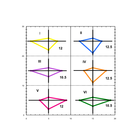
Figure 1: Demonstration that starting from 4 criteria the shape of the polygon based on the variable values leads to different areas; the toy values are $a=1,b=2,c=3,d=4$, leading to 6 possible polygons, but 3 different sizes; the areas values are given in arbitrary units.

Figure 2: A toy case of six criteria is presented in two sub-figures. The variables take values $a,b,c,d,e,f$ in both displays. Notice the disposition of the axes, whose arbitrariness concerns the discussion ground of the present study. A different disposition in the relative order of the axes leads to a different area for the hexagon.

3 The problem and its solution

Thus, the way to proceed goes as follows. First, take a survey with as many possible criteria which are needed for a population whatever its size. One may suppose, without loss of generality, that the choice is based on Likert scales, whatever the useful range $[0,5]$, $[0,7]$, $\dots$, $[0,20]$.

Notice that it could be of interest to consider the mean and standard deviation of the data distribution on each axis, such that one can obtain a possible ”universal comparison” of final rankings and hierarchies. If the statistical characteristics make sense, the measured values could be normalised or, at least, constrained to vary in an identical range. One could assume that all the values involved in the decision process belong to $[0,1]$. The value 0 is achieved in the worst situation for the considered parameter (bad realisation) and, accordingly, 1 is taken in the ”best choice” case. Nevertheless, such a scaling is not a fundamental request. Although of interest, the normalisation aspect is not further discussed and is left for further work.

Then, one reports the values on equidistant axes. These are disposed in a regular star-shaped network with a central node, the common starting point and identical angles between consecutive axes; the angle value obviously depends on the number of axes (criteria). The non-common nodes of the consecutive segments are connected. The resulting polygon has a number of sides identical to the number of evaluation parameters; the polygon is not necessarily regular; It can be considered made of triangles. If $N$ is the number of axes, the largest possible number of different polygons is $[(N-1)!/2]$. The number of different triangles is $N$!.

In this paper, let us focus on hexagons, since evaluation processes are very often associated to six different parameters.

In Fig. 2, we present an example for two hexagons out of 60 possible cases; let $a,b,c,d,e,f$ (e.g., $\in[0,1]$), the values of the six parameters. The surface of the resulting hexagon $\mathcal{S}$ can be easily computed. The evaluation score coincides with the value of $\mathcal{S}$, so that high $\mathcal{S}$ means high score. However, notice that $\mathcal{S}$ belongs to the range associated to the limiting cases $a=b=c=d=e=f=0$ (worst result of the evaluation process, with $\mathcal{S}=0$) and $a=b=c=d=e=f=1$ (best result of the evaluation exercise, with $\mathcal{S}=\frac{3\sqrt{3}}{2}$).

Clearly, the surface of the hexagons shown in Fig. 2 depends on how the segments are disposed: the values of the six measures are always $a,b,c,d,e,f$ but the placement of $c$ and $f$ have been reverted in both displays.

Let $\mathcal{S}_{1}$ and $\mathcal{S}_{2}$ be the surface of the hexagons in Fig. 2, (left) and (right), respectively. We have

$$\mathcal{S}_{1}=\frac{\sin{(\pi/3)}}{2}\left[ab+bc+cd+de+ef+fa\right]=\frac{\sqrt{3}}{4}\left[ab+bc+cd+de+ef+fa\right],$$

$$\mathcal{S}_{2}=\frac{\sin{(\pi/3)}}{2}\left[ab+bf+fd+de+ec+ca\right]=\frac{\sqrt{3}}{4}\left[ab+bf+fd+de+ec+ca\right];$$

in the case $b+d-e-a\neq 0$, one has that $\mathcal{S}_{1}=\mathcal{S}_{2}$, if and only if $c=f$.

Such a remark leads to the questionability of the evaluation exercise through polygons. Indeed, the resulting polygons, differently shaped according to the disposition of the axes, have different surfaces. This means that the evaluation is strongly dependent on how selection parameters are included in the graphical representation of the problem, as we do stress again.

To overcome such an inconsistency, whence in order to obtain a more indubitable scoring, we propose to take the average $\bar{\mathcal{S}}(a,b,c,d,e,f)$ of all the possible polygon surfaces, thus over all the possible dispositions of the axes, - here corresponding to 6 evaluation criteria:

$$\bar{\mathcal{S}}(a,b,c,d,e,f)=\frac{\sin{(\pi/3)}}{5!}\sum_{\mathbf{H}(a,b,c,d,e,f)}\left[x_{1}x_{2}+x_{2}x_{3}+x_{3}x_{4}+x_{4}x_{5}+x_{5}x_{6}+x_{6}x_{1}\right],$$ (5)

where

$$\mathbf{H}(a,b,c,d,e,f)=(x_{1},\dots,x_{6})\in\{a,b,c,d,e,f\}^{(6)}:x_{i}\neq x_{j},\text{ for each }i\neq j.$$

By construction, $0\leq\bar{\mathcal{S}}(a,b,c,d,e,f)\leq\frac{3\sqrt{3}}{2}$. Such a mean surface measure effectively does the intended job, i.e., providing a consistent score of the evaluated object whose six parameters (criteria) take values $a,b,c,d,e,f$.

This is consistent with the measure concept resulting into calculating the correlation between fluctuations in statistical physics, as found in linear response theory: see Appendix A. Examples of Applications are found in Appendix B.

4 Conclusions

In brief, the present paper aims at resolving a paradoxical situation when searching for an objective ranking procedure and subsequently observing some hierarchy through a set of criteria for some population. This sort of scientometrics practice is tied to considerations found in geometry and statistical physics, complementing aspects of research on opinion dynamics, in Galam’s numerous studies.

Observe the technical and somewhat philosophical frames, in the present ranking study. Decisions often concern rather small sub-systems, like, the funding of a project, the evaluation of a research group or of that an individual, at his or her hiring or promotion. Statistical laws cannot be immediately applied for such cases in which, due to the (very finite) size of the system, fluctuations which are not necessarily due to stochastic causes play a crucial role. Indeed, recall that scientific work is part of a social system; its actors are human beings. Moreover, statistics are like snapshots and do not often allow to predict the future very well! In practice, indeed, any newly introduced criterion or ”measure” will be met by the capacity of humans to interact and making decisions.

Without going back to the Bible and raising the question who is the just and who will be saved, - according to a single judge, it can be considered that the modern time of scientific reasoning on choice, - when several partners and judges are implied, goes back to Arrow [37]. He considered the preference aggregation problem, that is the problem of passing from a set of known individual preferences to a pattern of social decision making. His now often quoted theorem (with various wordings) has nevertheless shown that the difficulties met in the building process of preference aggregation are very general. The theorem implies that no rank order voting system can convert the ranked preferences of individuals into a community-wide (complete and transitive) ranking, beside also meeting a specific set of natural criteria.

In fact, why is it impossible to reach a choice? Usually, one constructs several filters and a priori decides on the order of their applications, liked in the decision tree (DT). That leads to a discussion on ranking the filters rather than the candidates.

Indeed, in the ”decision tree” (DT) scheme, due to the order of filtering criteria, the final choice is much biased. The order of filters is often adapted a priori  in order to select the final choice, e.g., a candidate, or maintain candidates in competition with others during the selection process, for hypocritical, political, or other reasons.

In opinionology, the selection process consists in projecting from a multidimensional space onto various planes, and finally finding the intersection of the distribution . There might not be any ”solution”. That further may mean that the set (of ”candidates”, ”events”, etc.), to be ordered, is either not to be ranked or that the filters are not appropriate.

Thus, we propose, starting from Galam and other socio-physicists considerations on the dynamics of choices, a procedure for obtaining the ”best choice” through an objective statistical physics method.

Of course, the situation might not be closed, since the choice of criteria is left for many discussions between agents, be they surveyees or surveyors, or other stakeholders.

Nevertheless, our arguing, after outlining elements of reflexion from information theory, geometry, surely complex systems, as found in sociophysics considerations, proposes a strong argument for calculating choice values. It is grounded in linear response theory : in the latter, as recalled in Appendix A, coefficients to be measured in laboratories and theoretically discussed, are defined through the correlations between the dependent variables; thus, we suggest to do the same in sociophysics, - to calculate all correlation functions implying the relevant variables, thereby avoiding an arbitrarily ordered set of criteria. In particular, this should be useful and meaningful in the modelling of opinion formation, processes dear to Prof. Galam. That methodology is missing in sociophysics previous work. Thus, such a LRT basis, rather easily implemented, should be leading to a more objective hierarchy of values ahead of selection processes.

Appendix A. Linear Response Theory

The linear response theory (LRT) was independently invented by Green [67, 68] and Kubo [69]: it describes the coefficients relating the effect of a perturbation on a thermodynamic system in equilibrium. The LRT has given a general proof of the fluctuation-dissipation theorem which states that the linear response of a given system to an external perturbation is expressed in terms of the correlations between fluctuations properties of the system in thermal equilibrium [70].

Kubo [69] considered the application of a magnetic field to an equilibrium system, and demonstrated that the magnetic susceptibility can be defined through the average of the correlations between the magnetic moment density fluctuations. The LRT also well applies to the description of the electrical conductivity or the thermal conductivity [71, 72], even if the system is characterised as being in a non-equilibrium state.

Consider a perturbation $B(t)$, e.g. a magnetic field, and search for the response of the system $M(t)$, i.e., the magnetisation. Usually one demands to obtain $M(t)=\chi B(t)$.

By analogy, in opinion formation and related rankings, one may consider that the ”response” is going to be the final score. It is extracted through the correlations between fluctuations of the values attributed to ”candidates” (in a wide sense, usually called ”agents”, - which might not be humans) through the various criteria. The mere fact that criteria are introduced for later agent ranking. is considered to induce ”perturbations” in the original system. The external field is the exogenous decision of introducing criteria.

Subsequently, one may consider that the external (field) perturbation is applied at some time $t_{0}$ to some (say) agents in some population; the ”population system” is in so doing moved away from its equilibrium, and is characterised through a non-equilibrium ensemble average. Thus, this leads to the measured score of each agent as a result of interactions in response to the opinion field perturbation, - as in most of Galam’s models.

In practice, considering a weak interaction with some external field, one can obtain the resulting score by performing an expansion in powers of the perturbation [67, 68, 69, 70, 71, 72]. The leading term in this expansion is independent of the field, but the next term describes the deviation from the equilibrium behaviour in terms of a linear dependence on the external perturbation through the correlations between the system fluctuations. The average score is the linear response function, i.e., the quantity that contains the (microscopic) information on the system and how it responds to the perturbing field.

Appendix B. Two examples

Among the many possible examples, in. the various research fields outlined in the Introduction and Conclusion sections, we have selected two examples which are likely of interest to many readers and researchers in physics, particularly in sociophysics. The first example concerns the promotion of researchers. The second example pertains to the evaluation of football (soccer) players. The former stresses how to reach a final ranking from ranks obtained through various filters. Three methods, outlined in the main text, are so compared. The latter example stresses that a meaningful ranking can be obtained from a final aggregation number based on measured values, analysed through correlations as proposed in the main text..

• Example 1. Researcher promotion.

  Consider for some illustration that 5 researchers (A, B, C, D, E) are applying for promotion. The relevant selection committee has decided to base its ranking of the value of the candidates on 4 criteria, related to the impact factor (IF) of the journal where a paper has been published. The committee calculates

  • the IF mean on the best 5 papers: $\overline{B5}$;

  • the iF mean on the worst 5 papers: $\overline{W5}$;

  • the IF mean on the oldest 5 papers: $\overline{F5}$;

  • the IF mean on the most recent 5 papers: $\overline{L5}$.

  The timing of the publication is considered irrelevant at this stage. The resulting mean values and the corresponding candidate rank is given in Table 1 for each criterion.

  Let the committee be (i) admitting that the ranks are more relevant than the scores, and (ii) the ranking of candidates be in descending order of the criteria scores.

  (i) It is immediately seen that candidate A has the highest $\overline{B5}$ (= 7.8) and $\overline{F5}$ (=7.8); author E has the maximum score on the last 5 ($\overline{L5}$) (= 7.60), but author B is not reaching any highest score, among these competitors, under any criterion. We may also remark that in this toy example, due to the nature of the evaluation, the candidate D lays at the bottom on each ranking, no matter the specific criterion is used. A difficulty arises in the need of ranking the 4 others, since each of them is a winner for at least one committee member (or criterion): A and C even winning twice, but on different criteria of course; B and E are twice ex aequo, but not near the top places. Thus, we have shown that different criteria lead to different rankings, but the more so the toy model implies that there is no obvious final choice as was indeed codified by Arrow’s theorem. Moreover, there is no indubitable hierarchy, along this simple aggregation process.

  (ii) Next, consider the Maximum Likelihood Rule (Sect. 2.1) method based on rankings, not on the scores, as given in Table 1). Recall that a MLR ordering is defined as one that minimises the total number of discrepancies among all the criteria in a pairwise preference scheme. The MLR ordering does not use any information about how much higher a candidate is ranked over another, but only a relative ordering. Practically, the method counts the pairwise preferences. The second step of the method consists in counting the number of times in which one candidate is ranked over another (from Table 1). In so doing, the MLR emphasises that the first-ranked choice wins against all other options in individual pairwise comparisons. Similarly, the MLR second ranked choice would win against all other options (except the first ranked), and so on. The present case outcome is reported in Table 2.

  It can be observed from Table 2 that D has the lowest number of potential preferences for promotion, whence is properly ranked as last. It can be remarked that the coalition of criteria formed only by $\overline{B5}$ and $\overline{L5}$ can be a decisive one on the ranking of E before B. However the rank relations between A and C are not so neat. Therefore, the selection committee would be faced with its self-application of Arrow’s theorem consequences, again.

  (iii) Finally, let us consider the newly proposed method. It boils down to calculating the surfaces of rectangular triangles and its subsequent averaging, - here for 3 types of polygons with 4 sides. Using Eq.(2), one obtains the results displayed in Table 3. It seems obvious that this ranking makes sense. Thereafter, one may conclude that the proposed method is more justified and advantageous than classical ones.

  	$\overline{B5}$		$\overline{W5}$		$\overline{F5}$		$\overline{L5}$
  A	7.80	1	3.20	2	7.80	1	3.20	4
  B	7.00	4	2.20	3	2.20	4	7.00	2
  C	7.60	2	3.60	1	7.60	2	3.60	3
  D	6.40	5	1.00	5	5.60	3	1.80	5
  E	7.60	2	2.20	3	2.20	4	7.60	1

  Table 1: Profile of 5 candidates (A, B, C, D, E) having published 10 papers, listed in chronological order, with the candidate evaluation through various criteria, proposed by examiners; the best score is underlined for each criterion; the corresponding rank is given; notations as in the text.

  	A	B	C	D	E
  A	$-$	3	2	4	3
  B	1	$-$	1	3	((0))
  C	2	3	$-$	4	(2)
  D	0	1	0	$-$	1
  E	1	((2))	(1)	3	$-$

  Table 2: MLR application: Table reporting how many $a_{i,j}$ times, according to Table 1, the candidate in row $i$ is ranked before the candidate in column $j$; parentheses indicate ex aequos.

  	$area\times 2$			$total$	$average$	rank
  A	12	15	15	42	14	1
  B	40	42	42	124	41.33	4
  C	16	15	15	46	15.33	2
  D	80	80	80	240	80	5
  E	24	25	21	70	23.33	3

  Table 3: Table reporting how 5 candidates (A, B, C, D, E) are ranked according to the proposed method; $area$ is the surface of each relevant 4 sided polygon; $total$ is the sum of the area of such polygons; $average$ is the average area.

• Example 2. Football (soccer) players.

  When this paper writing was being completed, we came across some related application which we are pleased to relate. It is about football players, ranking them on their ”market value”, ”potential”, salaries, age, and many statistical ”criteria”: see $https://sofifa.com/players$; or for teams: https://sofifa.com/teams. Another example of ”player value” can be found on internet sites like https:https://www.laliga.com/en-GB/player/robert-lewandowski on which 8 criteria are displayed. Radar picture comparisons can be created: https://www.laliga.com/en-GB/comparator/players?player1=witsel.

  In particular, e-players can form their own team, based on real players, considering six criteria, displayed on a regular hexagon thereafter transformed into a colourful pattern; e.g., see https://sofifa.com/player/183277/eden-hazard/230036/.

  The six skill measures, obtained through several sub-criteria, are given in Table 4. In brief, SHO: SHOOTING: determines finishing skill and shot power, including penalty success; PAS: PASSING: denotes ability to successfully pass the ball with vision; DRI: DRIBBLING: denotes ball control, agility and balance; DEF: DEFENDING: notes tackling and interceptions;, PHY: PHYSICALITY: notes strength and stamina, and aggressiveness; PAC: PACE: notes the speed and the acceleration of the player.

  Notice that it is not obvious to us how the ”overall note” is obtained. Since only one hexagon is shown, it is clearly one for which the axes are a priori chosen, whence are not conforming to our recommendations about a tentative ranking (of football players) upon some unique value which is resulting from some aggregation process.

  $"measure"$	skill:	SHO	PAS	DRI	DEF	PHY	PAC
  77	SHO	-	6237	6545	2695	4774	6083
  81	PAS	6237	-	6885	2835	5022	6399
  85	DRI	6545	6885	-	2975	5270	6715
  35	DEF	2695	2835	2975	-	2170	2765
  62	PHY	4774	5022	5270	2170	-	4898
  79	PAC	6083	6399	6715	2765	4898	-

  Table 4: The 6 skill variables considered for measuring the ”value” of E. Hazard, with their respective measure according to https://sofifa.com/player/183277/eden-hazard/230036/; the data in the matrix corresponds to the area (divided by $\frac{\sin{(\pi/3)}}{2}$, see Eq.(3)) of the 15 possible triangles, - to be arranged in 60 different hexagons.

  	$\nu$	min.	Max.	Total area	mean	Std Dev	skewness	kurtosis
  $sofifa$	6	2170	6885	29248	4874.7	1912.2	-0.4457	-1.4123
  LRT	60	28298	29600	1734432	28907	437.04	0.3076	-1.5345

  Table 5: Main statistical characteristics of the distribution of (i) top line: the 6 triangle areas forming the single hexagon in the $sofifa$ website, (ii) bottom line: the 60 possible hexagons areas characterising E. Hazard along the 6 skill axes, following the LRT method described in the text.

  Thereafter, in order to avoid useless decimals, we measure the area of triangles, whence of corresponding hexagons in $\sqrt{3}/4$ units; see Eq.(3).

  Consider one case in order to describe how the resulting aggregation player value is obtained, ahead of some selection process; consider E. Hazard. According to the mentioned web site, https://sofifa.com/player/183277/eden-hazard/230036/, his ”best overall = 82”. However, the average of his skill values equals 69.83, as easily obtained from the values given in Table 4 first column. Moreover, the latter Table reports the data corresponding to the area (divided by $\frac{\sin{(\pi/3)}}{2}$, see Eq.(3)) of the 15 possible triangles. For space saving, not all 60 relevant hexagons can be displayed, nor the whole list of their areas. For some completeness, the statistical characteristics of the polygon areas distribution is given in Table 5. The first line reports the characteristics for the distribution of triangle areas on the diagram displayed on https://sofifa.com/player/183277/eden-hazard/230036/; it corresponds to a mere $\nu=6$ axes diagram; the second line details the distribution of the $\nu=60$ hexagon areas considered along the present method. It is remarkable that the LRT result shows a much narrower distribution, thus a more convincing statistics. The sign of the skewness is also in favour of the LRT method.

  Not considering here a comparison with other players, we should point that such a comparison demands a final aggregation score. In order to have a universal rule, we suggest that the best is to measure the ”player hexagon area(s)” with respect to the perfect player, i.e., the largest regular hexagon. For the $sofifa$ and the LRT case, one obtains 0.4875 and 0.4818, respectively.

As a conclusion of this Appendix, notice that we have first debated on how to reach a hierarchical selection, through three methods, using numerical examples. The illustration is based on a toy case made of a set of 5 candidates applying for promotion through a 4 criteria selection process. Next, we have presented the whole scheme resulting in the aggregation score for a given individual examined through 6 values or criteria, along two methods.

We have stressed the objective advantages of the LRT based method in both examples.

Therefore, we can conclude from both toy cases here above, it seems to us, that the usability and the advantage of the LRT methodology both bring much support to considerations in the sociophysics interdisciplinary field searching for objective ranking, whence leading to a justified choice. We emphasise that the main justification is the use of correlation functions, as in LRT, i.e., a pertinent statistical physics theory basis.

References

- [1] Stauffer, D. (2000). Grand unification of exotic statistical physics. Physica A: Statistical Mechanics and its Applications, 285(1-2), 121-126.
- [2] Stauffer, D. (2004). Introduction to statistical physics outside physics. Physica A: Statistical Mechanics and its Applications, 336(1-2), 1-5.
- [3] Săvoiu, G., & Iorga-Simăn, I. (2012). Sociophysics: A new science or a new domain for physicists in a modern university. In G. Săvoiu (Ed.), Econophysics: Background and Applications in Economics, Finance, and Sociophysics. Academic Press, Oxford/Waltham.
- [4] Kutner, R., Ausloos, M., Grech, D., Di Matteo, T., Schinckus, C., and Stanley, H. E. (2019). Econophysics and sociophysics: Their milestones & challenges. Physica A: Statistical Mechanics and its Applications, 516, 240-253.
- [5] Grech, D., and Miśkiewicz, J. (Eds.). (2020). Simplicity of Complexity in Economic and Social Systems. Springer, Cham.
- [6] Galam, S., Gefen, Y., and Shapir, Y. (1982). Sociophysics: A new approach of sociological collective behaviour. I. mean‐behaviour description of a strike. Journal of Mathematical Sociology, 9(1), 1-13.
- [7] Galam, S. (2008). Sociophysics: A review of Galam models, International Journal of Modern Physics C, 19, 409–440.
- [8] Galam, S. (1997). Rational group decision making. A random field Ising model at T=0. Physica A: Statistical Mechanics and its Applications 238, 66-80.
- [9] Galam, S. (2004). Contrarian deterministic effects on opinion dynamics: ‘’the hung elections scenario”. Physica A: Statistical Mechanics and its Applications 333, 453-460.
- [10] Galam, S. (2013). Modeling the Forming of Public Opinion: an approach from Sociophysics. Global Economics and Management Review 18(1), 2-11.
- [11] Galam, S. (2014). Is It Necessary to Lie to Win a Controversial Public Debate? An Answer from Sociophysics. In: Matrasulov, D., Stanley, H. (eds.) Nonlinear Phenomena in Complex Systems: From Nano to Macro Scale (pp. 37-45). Springer, Dordrecht.
- [12] Galam, S. (2016). The invisible hand and the rational agent are behind bubbles and crashes. Chaos, Solitons & Fractals, 88, 209-217.
- [13] Galam, S. and Cheon, T. (2020). Tipping points in opinion dynamics: a universal formula in five dimensions. Frontiers in Physics 8, 566580.
- [14] Galam, S. (2022). Opinion Dynamics and Unifying Principles: A Global Unifying Frame. Entropy 24(9), 1201.
- [15] Biondi, Y., Giannoccolo, P., and Galam, S. (2012) Formation of share market prices under heterogeneous beliefs and common knowledge. Physica A: Statistical Mechanics and its Applications 391(22), 5532-5545.
- [16] Dhesi, G., and Ausloos, M. (2016). Modelling and measuring the irrational behaviour of agents in financial markets: Discovering the psychological soliton. Chaos, Solitons & Fractals, 88, 119-125.
- [17] Lehmann, D. R. (1971). Television show preference: Application of a choice model. Journal of Marketing Research, 8(1), 47-55.
- [18] Lambiotte, R., and Ausloos, M. (2006). On the genre-fication of music: a percolation approach. The European Physical Journal B-Condensed Matter and Complex Systems, 50, 183-188.
- [19] Camagni, R., Capello, R., and Caragliu, A. (2015). The rise of second-rank cities: what role for agglomeration economies?. European Planning Studies, 23(6), 1069-1089.
- [20] Novac, A., and Dumitrescu-Moroianu, N. (2020). Dynamic Model of Regional Convergence. Romanian Statistical Review-Suppl., 6, 49-60.
- [21] Rotundo, G., and Navarra, M. (2007). On the maximum drawdown during speculative bubbles. Physica A: Statistical Mechanics and its Applications, 382(1), 235-246.
- [22] Golubic, R., Rudes, M., Kovacic, N., Marusic, M., and Marusic, A. (2008). Calculating impact factor: how bibliographical classification of journal items affects the impact factor of large and small journals. Science and Engineering Ethics, 14, 41-49.
- [23] Cerqueti, R., Iovanella, A., and Mattera, R. (2023). Clustering networked funded European research activities through rank-size laws. Annals of Operations Research, https://doi.org/10.1007/s10479-023-05321-6.
- [24] Liu, N. C., and Cheng, Y. (2005). The academic ranking of world universities. Higher Education in Europe, 30(2), 127-136.
- [25] Florian, R. V. (2007). Irreproducibility of the results of the Shanghai academic ranking of world universities. Scientometrics, 72(1), 25-32.
- [26]
- [27] Taylor, J. M. (1982). The politics of aesthetic debate: the case of Brazilian carnival. Ethnology, 21(4), 301-311.
- [28] Mitchell, J. H., Haskell, W. L., and Raven, P. B. (1994). Classification of sports. Journal of the American College of Cardiology, 24(4), 864-866.
- [29] Ausloos, M., Gadomski, A., and Vitanov, N. K. (2014). Primacy and ranking of UEFA soccer teams from biasing organization rules. Physica Scripta, 89(10), 108002.
- [30] Malcata, R. M., Vandenbogaerde, T. J., and Hopkins, W. G. (2014). Using athletes’ world rankings to assess countries’ performance. International Journal of Sports Physiology and Performance, 9(1), 133-138.
- [31] Ficcadenti, V., Cerqueti, R., and Varde’i, C. H. (2022). A rank-size approach to analyse soccer competitions and teams: the case of the Italian football league “Serie A”. Annals of Operations Research, 385, 45-113.
- [32] Ausloos, M. (2023). Hierarchy selection: New team ranking indicators for cyclist multi-stage races. European Journal of Operational Research, 314(2), 807-816.
- [33] Ausloos, M. (2023). Shannon Entropy and Herfindahl-Hirschman Index as Team’s Performance and Competitive Balance Indicators in Cyclist Multi-Stage Races. Entropy, 25(6), 955.
- [34] de Condorcet, N. (1785). Essay on the Application of Analysis to the Probability of Majority Decisions. Imprimerie Royale, Paris.
- [35] Young, H. P. and Levenglick, A.A. (1978). A consistent Extension of Condorcet’s Election Principle. SIAM Journal on Applied Mathematics 35(2), 285-300.
- [36] Young, H. P. (1988). Condorcet’s theory of voting. American Political Science Review, 82(4), 1231-1244.
- [37] Arrow, K.J. (1950). A Difficulty in the Concept of Social Welfare. Journal of Political Economy 58(4), 328-346.
- [38] He, Y. and Deng, Y. (2023). Ordinal belief entropy. Soft Computing, 27, 6973-6981
- [39] Krawczyk, M. J., Wołoszyn, M., Gronek, P., Kułakowski, K., and Mucha, J. (2019). The Heider balance and the looking-glass self: modelling dynamics of social relations. Scientific Reports, 9(1), 11202.
- [40] Krawczyk, M.J. and Kułakowski, K. (2021). Structural Balance of Opinions. Entropy 23(11), 1418 (2021).
- [41] Columbu, G. L., De Martino, A., and Giansanti, A. (2008). Nature and statistics of majority rankings in a dynamical model of preference aggregation. Physica A: Statistical Mechanics and its Applications, 387(5-6), 1338-1344.
- [42] Munda, G. (2012). Choosing aggregation rules for composite indicators. Social Indicators Research, 109(3), 337-354.
- [43] Nehama, I. (2013). Approximately classic judgement aggregation, Annals of Mathematics and Artificial Intelligence, 68 , 91-134.
- [44] Pumain, D. (2006). Hierarchy in Natural and Social Sciences. Springer-Verlag, Cham.
- [45] Marfels, C. (1971). Absolute and relative measures of concentration reconsidered. Kyklos, 24(4), 753-766.
- [46] Bikker, J. A., and Haaf, K. (2002). Competition, concentration and their relationship: An empirical analysis of the banking industry. Journal of Banking and Finance, 26(11), 2191-2214.
- [47] Cowell, F. (2011). Measuring inequality. Oxford University Press, Oxford.
- [48] Young, H. P. (1995). Optimal Voting Rules, Journal of Economic Perspectives, 9(1) 51-64.
- [49] García, J. A., Rodriguez-Sánchez, R., Fdez-Valdivia, J., and de Moya-Anegón, F. (2014). A web application for aggregating conflicting reviewers’ preferences. Scientometrics, 99, 523-539.
- [50] Torres, R. (2005). Limiting dictatorial rules. Journal of Mathematical Economics, 41(7), 913–935.
- [51] Le Cam, L. (1990). Maximum likelihood: an introduction. International Statistical Review/Revue Internationale de Statistique, 58(2), 153-171.
- [52] Kemeny, J. (1959). Mathematics without numbers. Daedalus 88, 577-591.
- [53] Varela, L. M., and Rotundo, G. (2016). Complex network analysis and nonlinear dynamics. In Complex Networks and Dynamics. P. Commendatore et al. (eds.) Lecture Notes in Economics and Mathematical Systems, vol. 683, pp. 3-25. Springer, Cham.
- [54] Lambiotte, R., and Ausloos, M. (2007). Coexistence of opposite opinions in a network with communities. Journal of Statistical Mechanics: Theory and Experiment, 2007(08), P08026.
- [55] Hwang, C. L. and K. Yoon, K. (1981). Multiple Attribute Decision Making: Methods and Applications. Springer-Verlag, New York.
- [56] Yoon, K. (1987). A reconciliation among discrete compromise situations. Journal of the Operational Research Society 38 (3), 277–286.
- [57] Hwang, C. L., Lai, Y. J., and Liu, T. Y. (1993). A new approach for multiple objective decision making. Computers and Operations Research, 20(8), 889-899.
- [58] Lai, Y. J., Liu, T. Y., and Hwang, C. L. (1994). Topsis for MODM. European Journal of Operational Research, 76(3), 486-500.
- [59] Parida, P.K., Mishra, D., and Behera, B. (2017) A New Approach for Selection of Candidate by TOPSIS Technique. Journal of Ultra Scientist of Physical Sciences-Section A (Mathematics), 29(12), 541-546.
- [60] Chakraborty, S., Chatterjee, P., and Das, P. P. (2024). Technique for Order of Preference by Similarity to Ideal Solution (Topsis). In Multi-Criteria Decision-Making Methods in Manufacturing Environments, (pp. 85-97). Apple Academic Press.
- [61] Fagin, R. (1974). Generalized first-order spectra and polynomial-time recognizable sets. In Karp, R. M. (ed.). Complexity of Computation: Proceedings of a Symposium in Applied Mathematics of the American Mathematical Society and the Society for industrial and Applied Mathematics, SIAM–AMS Proceedings. 7, 43–73.
- [62] Kohler, R. (1981). A segmentation system based on thresholding. Computer Graphics and Image Processing, 15(4), 319-338.
- [63] Morariu, N., Iancu, E., and Vlad, S. (2009). A neural network model for time series forecasting. Romanian journal of economic forecasting, 4(2009), 213-223.
- [64] Ho, T. K., Hull, J. J., and Srihari, S. N. (1994). Decision combination in multiple classifier systems. IEEE Transactions on Pattern Analysis and Machine Intelligence, 16(1), 66-75.
- [65] Alwin, D. F., and Krosnick, J. A. (1985). The measurement of values in surveys: A comparison of ratings and rankings. Public Opinion Quarterly, 49(4), 535-552.
- [66] Sanchez, M. E. (1992). Effects of questionnaire design on the quality of survey data. Public Opinion Quarterly, 56(2), 206-217.
- [67] Green, M. S. (1952). Markoff random processes and the statistical mechanics of time‐dependent phenomena. The Journal of Chemical Physics, 20(8), 1281-1295.
- [68] Green, M. S. (1954). Markoff random processes and the statistical mechanics of time‐dependent phenomena. II. Irreversible processes in fluids. The Journal of Chemical Physics, 22(3), 398-413.
- [69] Kubo, R. (1966). The fluctuation-dissipation theorem. Reports on Progress in Physics, 29(1), 255-284.
- [70] Andrieux, D., and Gaspard, P. (2004). Fluctuation theorem and Onsager reciprocity relations. The Journal of Chemical Physics, 121(13), 6167-6174.
- [71] Mori, H. (1965). Transport, collective motion, and Brownian motion. Progress of Theoretical Physics, 33(3), 423-455.
- [72] Ausloos, M. (1978). Relation between the Mori-Green-Kubo formulae and their Boltzmann approximation for electronic transport coefficients. Journal of Physics A: Mathematical and General, 11(8), 1621-1632.