SegNet: A Segmented Deep Learning based Convolutional Neural Network Approach for Drones Wildfire Detection

Abstract

This research addresses the pressing challenge of enhancing processing times and detection capabilities in Unmanned Aerial Vehicle (UAV)/drone imagery for global wildfire detection, despite limited datasets. Proposing a Segmented Neural Network (SegNet) selection approach, we focus on reducing feature maps to boost both time resolution and accuracy significantly advancing processing speeds and accuracy in real-time wildfire detection. This paper contributes to increased processing speeds enabling real-time detection capabilities for wildfire, increased detection accuracy of wildfire, and improved detection capabilities of early wildfire, through proposing a new direction for image classification of amorphous objects like fire, water, smoke, etc. Employing Convolutional Neural Networks (CNNs) for image classification, emphasizing on the reduction of irrelevant features vital for deep learning processes, especially in live feed data for fire detection. Amidst the complexity of live feed data in fire detection, our study emphasizes on image feed, highlighting the urgency to enhance real-time processing. Our proposed algorithm combats feature overload through segmentation, addressing challenges arising from diverse features like objects, colors, and textures. Notably, a delicate balance of feature map size and dataset adequacy is pivotal. Several research papers use smaller image sizes, compromising feature richness which necessitating a new approach. We illuminate the critical role of pixel density in retaining essential details, especially for early wildfire detection. By carefully selecting number of filters during training, we underscore the significance of higher pixel density for proper feature selection. The proposed SegNet approach is rigorously evaluated using real-world dataset obtained by a drone flight and compared to state-of-the-art literature.

 
Video of the experiment: Click Here
 

I Introduction

Our lives rely heavily on the resources that forests provide. They are regarded as the planet’s lungs because they filter the air by adding oxygen (O2) and lowering the high levels of carbon dioxide levels (CO2). They serve as homes for a variety of animals and can be utilized to shield crops from the wind. Additionally, they clear the water of the majority of pollution-causing agents [1, 2]. Due to the numerous jobs and higher revenues that forests create, countries’ economies are improved. Forests have a profound impact on humanity by providing essential ecosystem services. They purify air, regulate climate, protect against natural disasters, and support biodiversity. Additionally, forests offer resources like timber and medicines, while promoting recreation and cultural heritage, highlighting their critical role in sustaining human well-being and the planet. Forest fires, often exacerbated by factors like climate change and human activity, have devastating effects on ecosystems, communities, and the environment. Forest fires, raging with increasing frequency and intensity, inflict profound damage. Ecologically, they destroy vital habitats, decimate wildlife populations, and disrupt ecosystems. Native flora and fauna struggle to recover, and invasive species often take hold in the aftermath. Fig. 1.(a) shows the global tree cover loss occurred between the years 2001 to 2022 [3]. Red dots are the areas effected by forest fires, few of which are under serious efforts of restoration. Communities near forests face immediate peril, with lives and homes in jeopardy. Firefighters risk their lives battling infernos. Smoke and air pollution pose serious health threats, especially to vulnerable populations. Evacuations disrupt livelihoods and cause psychological trauma. Economically, the costs are staggering. Firefighting expenditures soar, and losses in timber, agriculture, and tourism industries mount. Long-term, diminished soil fertility hinders agriculture, and reduced water quality impacts communities downstream. Environmental repercussions extend globally. Forest fires release vast amounts of carbon dioxide, contributing to climate change. This, in turn, exacerbates conditions conducive to more frequent and severe fires in a vicious cycle. Fig. 1.(b) shows the share of total global forest area across continents [4].

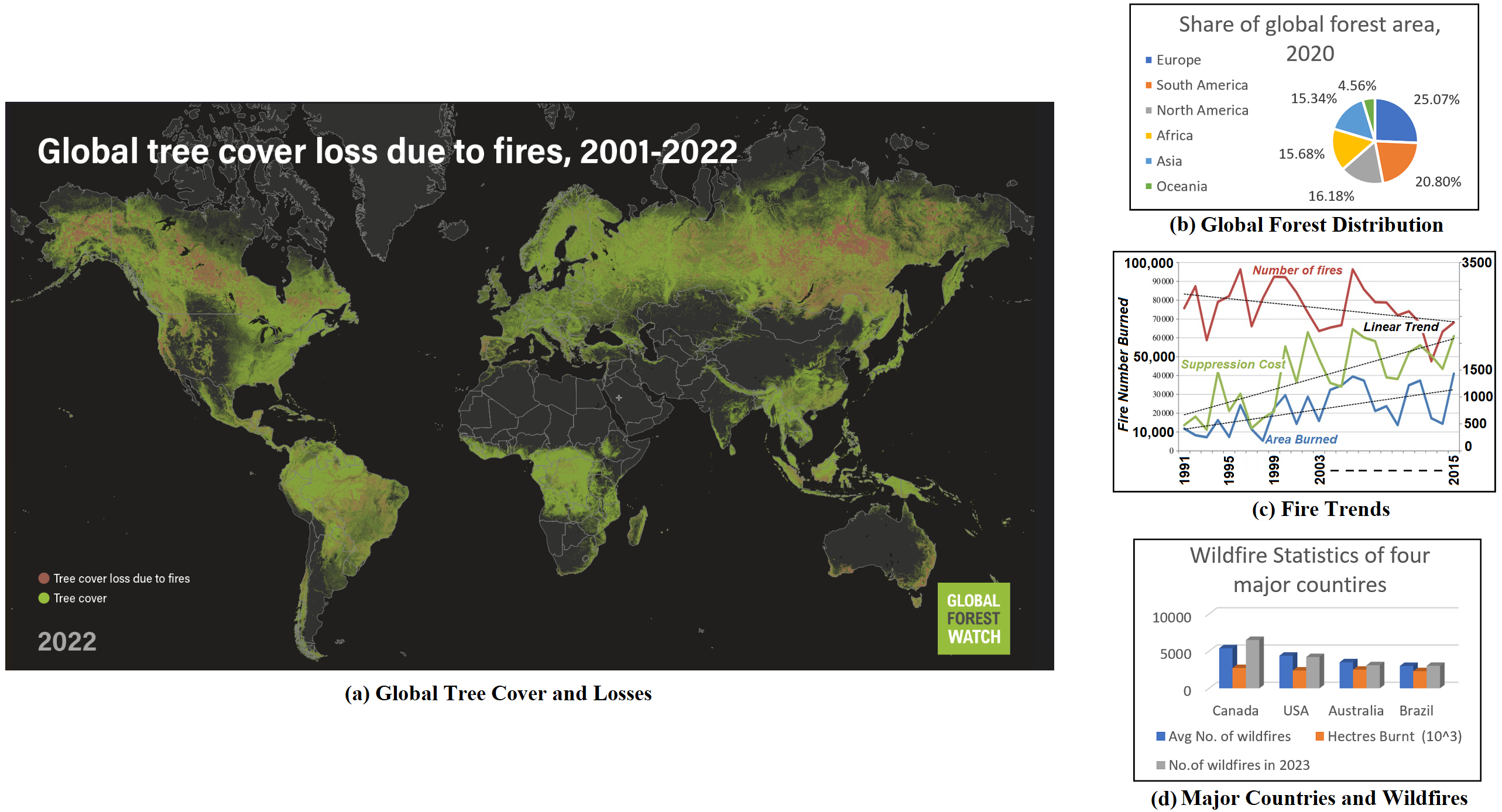
Figure 1: Wildfires is a global and growing threat: (a) Global tree cover loss due to forest fires, 2001-2022 (courtesy to [3]). (b) Global distribution of forest land [4]. (c) Number of fires and suppression cost with area burnt along with linear trend lines from 1991-2015 (National Interagency Fire Center [5]). (d) Wildfire metrics of Canada, USA, Australia, and Brazil [6].

I-A Related Work

Preventing and mitigating forest fires requires concerted efforts. Strategies include controlled burns, firebreaks, and early warning systems. Additionally, addressing climate change and promoting sustainable land management are crucial to curbing the catastrophic effects of these infernos. In recent years, a lot of forest fires have been taking place and because of wildfire’s terrifying effects on the economy, human health, and the environment, forest accidents have emerged as one of the greatest risks to humanity. Every year, more than $8,000$ fires burn an average of more than 2.1 million hectares in only Canada [7]. Wildfire frequency and total burnt area alone in the western US have surged by $400\%$ during the past ten years [8]. The wildfire in Australia was the most devastating fire in 2020, resulting in numerous losses, including the destruction of more than $1,500$ homes, the death of around $500,000$ animals, and the burning of more than 14 million acres [9]. Other destructive wildfires have occurred, causing enormous losses. For example, the 2018 California fire and the 2019 Amazon rain forest fire both burned millions of acres of land. Based on data in the National Forestry Database, over $8,000$ fires occur each year, and burn an average of over 2.1 million hectares in Canada [7]. Looking at the linear trends in Fig. 1.(c), the inclining slope of suppression costs depict an ever-growing effort to curb forest fires [5]. Although the steep inclining slope of burnt area does not justify the slow declining rate in number of fires despite the technological advances (cost slope). As proved by the wildfire cases stated earlier and the statistics from Fig. 1.(d) wildfire occurrences have caused increased damage every passing year throughout the decade. Canada, USA, Australia, and Brazil [6] are amongst the top hotspots for frequent wildfires. Accordingly, from Fig. 1 it is notable that overall wildfires are in a growing uptrend and novel solutions are of great importance and urgent demand.

Sensors and sensor fusion are standard part for early prediction/detection and therefore risk mitigation and management [10, 11, 12]. Typically, sensors like gas, smoke, temperature, and flame detectors are used to identify wildfires [13, 14, 15, 16, 17]. However, these detectors have a number of drawbacks, including slow response times and limited coverage areas [13]. Traditional fire detection methods are now being superseded by vision-based models because of their accuracy, wide coverage regions, low error probability. Moreover, vision-based techniques are distinguished with compatibility with current camera surveillance systems which can be easily implemented [18, 19]. In order to create precise fire detection systems, researchers have proposed numerous cutting-edge computer vision approaches over the last years, including Infra-Red (IR) images [19, 20]. As a result, Unmanned Aerial Vehicle (UAV) or drone systems have recently gained popularity and been used to combat and find the forest’s deep wildfires. Additionally, by combining this with Deep Learning (DL) methods, it has made remarkable progress [21]. The color of the wildfire and its geometrical characteristics, such as angle, shape, height, and width, are detected using Deep Learning (DL)-based fire detection algorithms. Their findings are fed into models of fire propagation [21, 22]. The effectiveness of these approaches for identifying and segmenting forest fires from UAV photos, in a real-life case, is yet unknown and to-date a challenging open problem. In particular, in the light of several difficulties that must be addressed, such as the tiny object size, the complexity of the backdrop, and the image deterioration and high computational cost [23, 24].

Several research efforts have been established concerning forest wildfire detection and prediction [25, 26, 27]. The research focus and implementation range from fixed to mobile solutions. Although mobile solutions have gained the support of many researchers as it outweighs its counterpart considering their advantages. Static solutions often deal with watchtowers that can be expensive to install [25] and carry the risk of being damaged by the fire itself, adding unnecessary repair costs on top. They are also restricted by the field of vision and obstruction of vision by complete or partial forest canopies. Mobile solutions such as UAVs can provide data in the form of images from different angles considering their flexibility to maneuver in the six degrees-of-freedom (6 DoF) [26]. Nowadays, several researchers consider a similar approach to solving this problem which go through the following steps: (1) Data Acquisition System: acquiring data using UAV sensors and cameras; (2) Data Processing Onboard: processing data with onboard microchips with learning algorithms; (3) Data Transmission/Receiving System: data is either transmitted to or received by on-ground equipment for further studies of data; and (4) Notifying Concerned Authorities: the wildfire management authorities are informed to make accommodations for further actions required [27].

I-B Persisting Challenges

For any real-time wildfire detection algorithm both the space and time resolutions are important. Stationary imagery has good time resolution but low spatial resolution. This is because the satellite body or watch tower can house a heavy, high performing GPU to process faster decreasing the processing times. Although, dispersion of light at various different angles, information in each pixel and environmental factors like fog, cloud cover, etc, hinder satellite’s vision capabilities resulting in low spatial resolution. On the contrary, mobile imagery consists of good spatial resolution but has poor time resolution. Thus, drone or rover imagery with conventional fire detection methods (smoke sensors, temperature sensors, etc) are not practically effective in real-time scenarios. Limitations in this area of research are plenty, these prove to be an obstacle for any researcher to fluently conduct their study. One such case would be the selection of Graphics Processing Units (GPU) since computational burden is a key element. High powered GPUs are not feasible as they have higher mass and volume, which are not preferred due to the limited weight capacity of drones. One other such limitation that is often overlooked is the problem of detecting forest fires during the fall season. Sugar maples in Canada or trees from the Laurel family around the globe turn orange-red in the fall season rendering any pixel color-based image classification technique ineffective, increasing the number of false alarms.

In case of any DL network, density of network is directly proportional to the delay caused in perceiving an image and classifying the image as fire or non-fire. Generally, a denser neural network increases the accuracy of the predictions due to increased processing of image feature pool. Although, for a real-time application, the algorithm must contain fewer dense layers for faster processing speeds and this must be carried out without having to compromise on the accuracy. Limited dataset of wildfire images available is one such gap that is slowing down the development of wildfire detection. With scarce resources of images available on the internet and real-life drone footage, capturing the aerial shot of wildfire, requiring government permissions to shoot and use, researchers have turned their focus on either augmenting the dataset or increasing the efficiency by using new enhanced algorithms. Datasets are being appended with newer synthetic images using Generative Adversarial Networks (GANs) [28], where a real non-fire image is translated into a modified image with fire. This also helps with creating wildfire datasets for YOLOv3 [29] format with localization and bounding box coordinates of fire within the image. Frame to frame capture of images from a wildfire video can produce large number of images but these lack in diversity of data which could cause overfitting to occur. Flames and smokes are amorphous in nature and difficult to label. Thus, to expertly annotate each image can take huge amounts of time. Therefore, the use of algorithms such as YOLOv3 [29] or faster Region-based Convolutional Neural Network (R-CNN) [30] becomes limited due to the lack of labeled and formatted data for training and testing of these algorithms.

I-C Modern Machine Learning Approaches

DL techniques have been popular over the past few decades as alternate strategies for difficult issues, such as the management and forecast of wildfires. The work in [22] reported a comparison research using Artificial Neural Networks (ANN) and Local Regression (LR) to map fire susceptibility, coming to the conclusion that ANN outperformed LR. A comparison of a deterministic approach and two Machine Learning (ML) techniques-Radio Frequency (RF) and extreme learning machine was provided by [31, 5, 32, 33]. The results of this investigation showed that the three techniques performed equally, emphasizing the advantage of both stochastic methods in that they are data-driven and, as a result, independent of prior information. Support Vector Machine (SVM), RF, and Multi-layer Perceptron (MLP), three ML-based approaches, were evaluated in a further comparison research by [34], with the MLP achieving the highest accuracy score [35]. Three techniques were employed by [36] for multi-hazard modeling (namely snow avalanches, floods, wildfires, landslides and land subsidence). Generalized Linear Model (GLM), SVM, and functional discriminant analysis were the approaches used. GLM produced the best results for predicting the risk of wildfires, closely followed by the other two. The work in [37] mapped fire susceptibility using the General Additive Model (GAM), Multivariate Adaptive Regression Spline (MARS), SVM, and the ensemble GAM-MARS-SVM. SVM was shown to be the least accurate approach out of these, whereas the ensemble had the best predictive accuracy. Most of the research is dealt with Convolution Neural Networks (CNN) and its variants, Single Shot Multi-Box Detector (SSD), U-shaped encoder-decoder network (U-Net), and deep Lab [29].

Some other less popular but effective learning algorithms include Long Short-Term Memory (LSTM), Deep Belief Network, and Generative Adversarial Network [28]. These algorithms are not preferred as they require powerful hardware which is difficult to house in a mobile UAV. The additional pieces of hardware add to the weight of the UAV creating a problem in terms of flight and control [38]. The use of remote compact cameras on UAVs outweighs the performance of the images taken by satellites due to their capacity to capture higher pixel density images from different angles. A tiny fire spot or extreme dryness of the objects would be almost impossible to spot using the images by satellites. Hence, to train the model better and to yield better results, mobile cameras are used. Additionally, the significance of the dataset has been consistently stressed to enhance the performance of the model since neural networks cannot be applied to untrained scenarios. Because it is difficult to detect smoke during the night and because the color and texture of smoke during model verification are too similar to other natural phenomena like fog, clouds, and water vapor, algorithms that rely on smoke detection typically have issues like high false alarm rates [39].

I-D Contributions

In this paper we address the problem of time resolution for UAV drone imagery along with limited dataset available on wildfires around the world using a proposed Segmented Neural Network (SegNet) selection approach based on DL reducing the total feature map. This novel SegNet technique contributes the following to robotic wildfire surveillance systems: (a) Increased processing speeds enabling real-time detection capabilities for wildfire in shorter period of time when compared to the existing cutting-edge solutions (e.g., [40, 41]); (b) Increased detection accuracy of wildfire which is confirmed through training, testing, and validation; (c) Introducing a new direction for image classification of amorphous objects which can add significant insight to fire, water, smoke, etc; and (d) Improved detection capabilities which can be potentially employed for early wildfire detection.

I-E Structure

The rest of the paper is organized as follows: Section II problem formulation, dataset preparation, data augmentation, and scaling issues. Section III illustrate the research methodology and segmentation. Section IV presents workflow, challenges, and mitigation. Section V illustrate results of the proposed SegNet approach in comparison to state-of-the-art literature. Finally, Section VI summarizes the work.

II Problem Formulation

The rapid advancements in Artificial Intelligence (AI) have catapulted it into one of the most swiftly evolving fields in applied science. However, amidst this complexity, researchers striving to emulate the intricacies of the human brain have crafted algorithms so sophisticated that they present unique challenges, particularly in their integration into the engineering sector. In the realm of robotics engineering, these challenges become evident. One of the significant hurdles stems from the complexity of machine learning models, which demand powerful computational processing. The current technological landscape grapples with a limitation: the lack of powerful, robust yet lightweight processing systems that can be seamlessly integrated into mobile robots. Considering drones or rovers, for instance. Equipping them with hefty, powerful processors is unfeasible, as these components are often heavy and can hamper the mobility and energy efficiency of these autonomous devices. Moreover, the cost factor amplifies the issue; these potent processing systems are expensive to produce, rendering them economically unviable for mass production. This becomes a critical concern, especially in the context of wildfire detection across extensive land masses. The application of complex machine learning algorithms on relatively weaker processors exacerbates the problem. While using less powerful processors in an attempt to mitigate the weight issue, the computational time required for running intricate algorithms becomes substantial, rendering these processors ineffective in real-time applications. Consequently, there arises a pressing need for a novel approach in machine learning—one that can provide real-time decision-making capabilities in the realm of wildfire detection. This necessity is steering researchers towards innovative solutions, emphasizing the urgency to bridge the gap between the robustness of algorithms and the limitations of current processing technologies in the pursuit of efficient and timely wildfire detection systems.

II-A Dataset and Preparation

Some images in the dataset might prove to counter the ideology being pursued in this research paper, that is, to subject the model to select features of fire like smoke, amorphous shape of the fire, color and brightness, etc (see Fig. 2). Some images contain environmental factors like fog and mist and can be misrepresented by the model such as smoke caused by fire. This eventually yields false positives during testing of the model. Some images that were acquired in the fall season often contain trees that have the fall coloring, that is, they turn into hues of orange, red and maroon. These hues of colors are similar to the colors of flame which are challenging. Thus, the model might, when trained with fall season images, classify an image with fire as non-fire attributing the fire image to be a fall season colored tree.

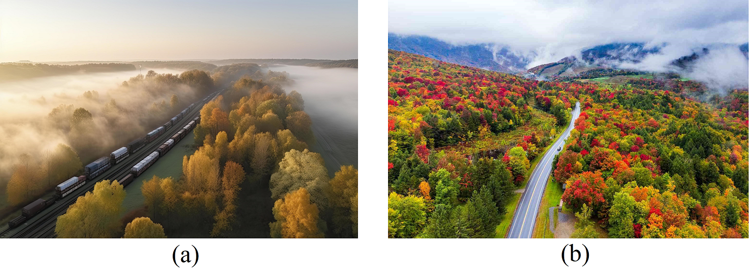
Figure 2: Environmental challenges: (a) Images with fog can be misclassified as smoke caused by wildfire, and (b) Red trees in the forest could yield undesired false results by model due to misclassification of the red spots (trees) in the image [42].

II-B Segmentation vs Complete Image

(a) Complete image.

(b) Segmented image.

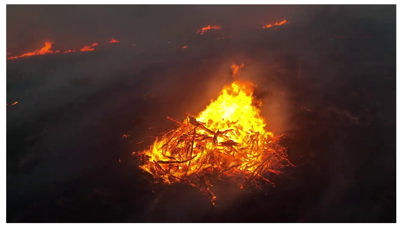
(c) Normal image.

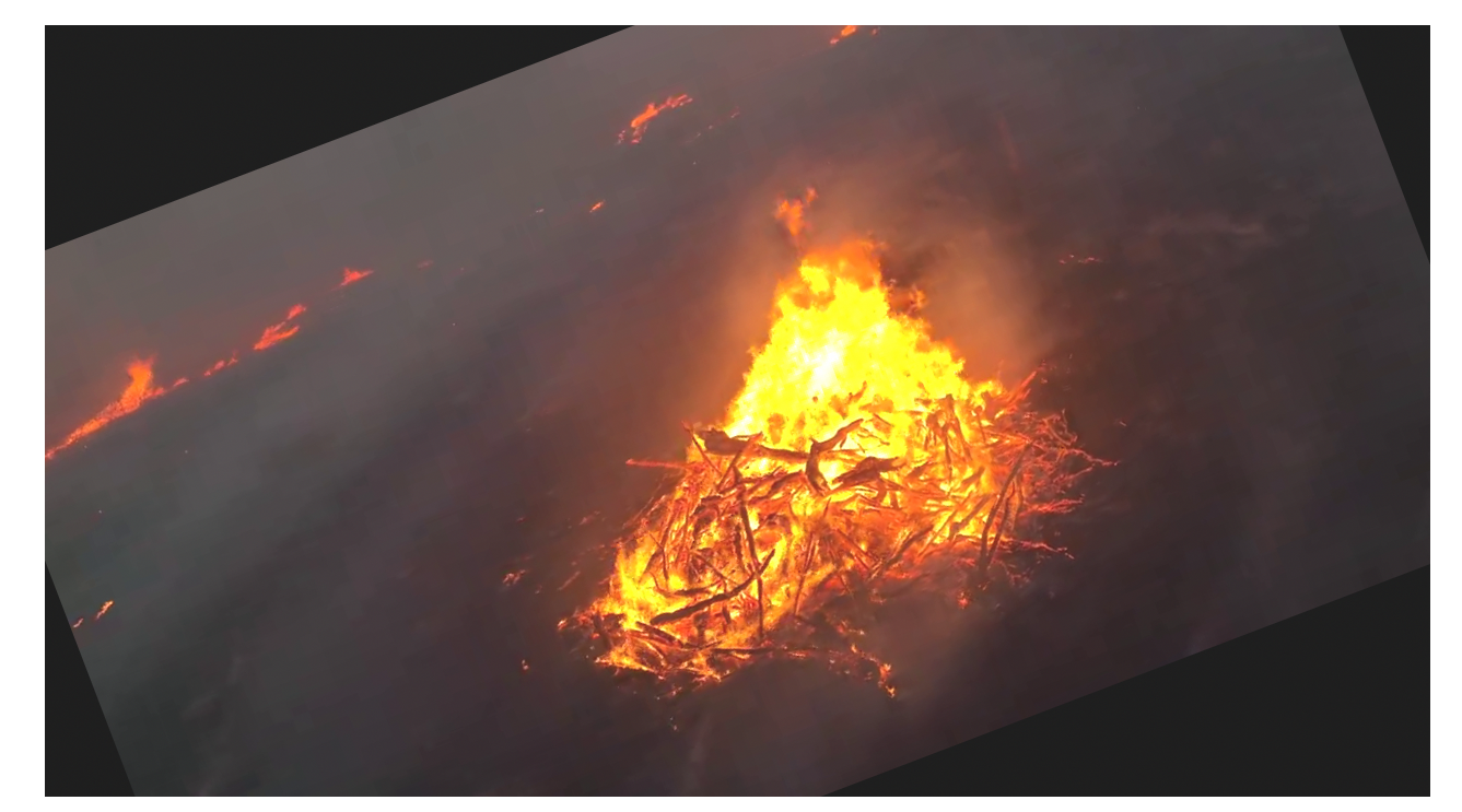
(d) Augmented image.

(e) No scaling.

(f) Rescaling introduced.

Figure 3: Dataset and preparation: (a) flames in a complete image, (b) flames in a segmented image, (c) flames in normal image (courtesy to WXChasing), and (d) flames in an augmented image, (e) no scaling (courtesy to Bloomberg), (f) Loss of information when scaling an image’s resolution.

Data for this classification problem is often subjected to limitations in the form of availability and proper labeling of classes. It is often stated by researchers [43], that lack of proper dataset for wildfires, unlike some other applications that include weather forecast, stock market predictions, models built around NLP like chatbots and smart AI assistants, has always limited the approach towards addressing this problem using various different state of the art techniques. Techniques like YOLOv3, R-CNN require training datasets with predefined bounding boxes around the class being investigated. Faster R-CNN as stated by [30] has proven to yield faster speeds in processing with high accuracy although the variability of training dataset is difficult to achieve due to limited dataset with bounding boxes available. Thus, in this research a custom dataset is used to train the model comprising of both complete images and segmented images (visit Fig. 3.(a) and 3.(b)). Each complete image can be broken down into 12 different segmented images. It is important to downsize the complete image from a resolution of $1280\times 720$ pixels to $320\times 240$ pixels. This is performed by using the PILLOW library available in the python environment. The combination of complete images and segmented images allow for the model to look for features of flame as a complete and incomplete demonstration.

II-C Data Augmentation

To improve dataset accuracy, various techniques were used to create diverse data. The initial model showed high accuracy in training but struggled during validation, indicating overfitting. To tackle this, artificial images were made through augmentation, preventing the model from focusing too much on specific examples. This helped the model recognize broader patterns and reduced the risk of memorizing isolated instances. The augmentation also addressed real-world challenges like different lighting conditions and viewpoints, common in practical scenarios throughout the year. Techniques including rotation, translation, scaling, brightness adjustment, and the introduction of Gaussian noise were tactically applied [44, 45]. These methods collectively fortified the model’s adaptability, enabling it to navigate through various input scenarios with resilience and precision (visit Fig. 3.(c) and 3.(d)). By incorporating these augmentation strategies, the model has not only become adept at handling diverse and nuanced data but also emerged as a robust tool for subsequent analyses and predictions. The dataset, enriched through these interventions, provided a solid foundation for the model to generalize patterns effectively, ensuring its applicability in real-world situations. This meticulous approach not only elevated the model’s training accuracy but also its validation accuracy.

II-D Scaling Issues

In Fig. 3.(e) and 3.(f), two different pixel sizes of the same shot of wildfire are taken. An image with $320\times 240$ pixels (on the left) and an image with $1280\times 720$ pixels (on the right). Same segments of the both these images are extracted which have the same area covered. The image with higher pixel density exhibits sharper image contrary to the image with lower pixel density which exhibits loss of information. This can be observed by looking at the trees in the environment. The shape and texture are dull when a lower pixel size is considered. This loss of information might result in improper filter selection during training effecting the accuracy of the model. Early detection of wildfire contains detection of a small fire spot and thus having higher pixel density is important and necessary.

III Methodology

CNNs have always been on the forefront when it comes to image classification problems. This is mainly due to the fact that CNN works with the use of several different filters to extract features out of an image [46]. Feature extraction and engineering is a domain in deep learning processes that has gained specific interest of lately. Yet, there is still a lot of development and understanding required about the same. This paper focuses on introducing a new practice of feature reduction in an image. In fire detection algorithms developed for data in the form of live feed data focuses on several features that cannot be assessed in an image classification algorithm. The constant flickering and moving pixels in the video data presents a quick solution for detection. Although this method falls behind in time resolution. In this paper we focus on image feed rather than video feed. The field of image classification has seen a lot of development towards improving the accuracy of detection. Very little focus has been put towards improving processing times to make real time detection effective. This algorithm focuses on reducing the number of features in the input image. This is done by segmentation of image. Any image feed when fed into the neural network, especially CNN, contains numerous features. These features could be anything ranging from objects and environment. These can be further divided into distinctions such as shape of the object, color of the object, texture of the object or how the object interacts with the environment. When in neural network convolutions are carried out by the filters, the product received is known as a feature. The collection of such features produced by various filters is known as a feature map. Higher number of image pixels translate to richer information about the image. More information then translates to higher number of total relevant features in the image.

$$\text{Number of pixels in image}\propto\text{information in the image}$$

$$\text{Image information}\propto\text{Number of discrete features}$$

For every engineering problem, choice of number of features in feature map changes. Some applications like anomaly detection in mechanical parts in a factory requires high pool of feature map to properly distinguish between different types of manufacturing defects. Similarly for wildfire detection problem a larger feature map enables capturing of the fire and its characteristics but negatively effects the training stage. A larger feature map requires a larger dataset with highly varying images of fire and non-fire which is neither easily available nor can they be effectively procured. An insufficient dataset while training the algorithm with larger feature map ends up with underfitting of the model. Data augmentation techniques also do not provide any better results as it leads to overfitting of the data. This is one of the main reasons for researchers using images of $256\times 256$ image size which results in significantly smaller feature map. This also results in loss of information.

III-A Segmentation

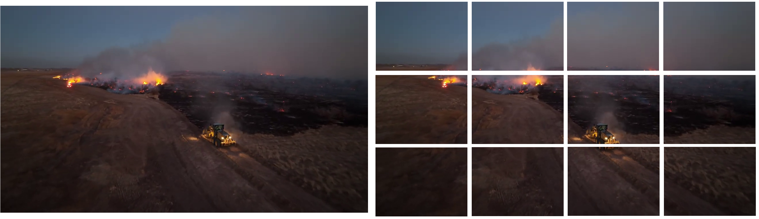
Figure 4: Segmentation of a complete image into twelve segmented images avoids loss of critical information and enables fire spots to be the prominent feature in the segmented image for better feature detection and selection. This approach can only be implemented on objects, under detection, that are amorphous in nature (do not exhibit a consistent shape or form).

Thus, in this paper we propose a solution using the segmentation technique of a wildfire image. In this technique, a high pixel image is broken down into several pieces. These pieces are equal in pixel size and are considered as different images. When any image is cut into pieces, that can be concatenated to form the original image, information is not lost. It is important to note that several objects in the image may lose their integrity in terms of their shape. For example, in Fig. 4, a tractor has lost its integrity of shape as it is segregated into two different images (body is in one image and the tires are in the other). This could hinder the algorithm’s capability to detect that object. Classification problems that involve morphous object’s detection, for an instance, an image of a person, are hard to deal with due to the same aforementioned reason. Thus, this technique is not useful for detection of fixed shaped objects. Flames, on the contrary, are amorphous in nature, that is, they do not possess a fixed shape or form. They can be found in different shapes, forms, color and intensity. This amorphous nature of fire enables this segmented image approach of this paper’s algorithm. Number of segments to be made of an image is dependent on the pixel size of the original image and the required processing speeds. Smaller the pixel size of segment of an image, faster is the processing speed involved. In this paper, original image pixel size of $1280\times 720$ is used in the dataset. These images are segmented into 12 segments where each segment is $320\times 240$ pixels pieces.

$$\frac{\text{Width of original image}}{\text{Number of vertical segments}}=\frac{1280}{4}=320\text{ pixels}$$

$$\frac{\text{Height of original image}}{\text{Number of horizontal segments}}=\frac{720}{3}=240\text{ pixels}$$

$$\text{Total number of segmented images}=4\times 3=12$$

Segmentation of images into smaller pieces cause two positive outcomes. First, in early wildfire images, flames become a prominent feature of one of the segmented-images. This, makes it easier for algorithm to detect flames and smoke resulting in increased accuracy for early wildfire detection. Second, processing speeds for these segmented-images will now increase as number of pixels of input image decreases (less computations to be performed as compared to when original image is used as input image). When integrating this algorithm within a UAV drone equipped with a 720p camera, the feed recorded would be in the form of a video. This video feed is broken into frames (images) so it can be compatible to be fed into the algorithm for classification. A 60 fps, 720p camera, records 60 frames of $1280\times 720$ pixel size every second. All these 60 frames are not relevant as they are a mere copy of each other at different angles, considering that UAV is under motion. Fig. 5 presents the proposed SegNet architecture for early wildfire detection (needs to be shifted to the end of SegNet Architecture). These frames prove to be useful for training of the model but not for execution. Thus, selecting a frame every 20 frames in a second, helps lower computational costs and speed up processing. This also provides time for additional supplemental programs on UAV, for example, fire alert signaling process to send results to respective authorities for any follow up action.

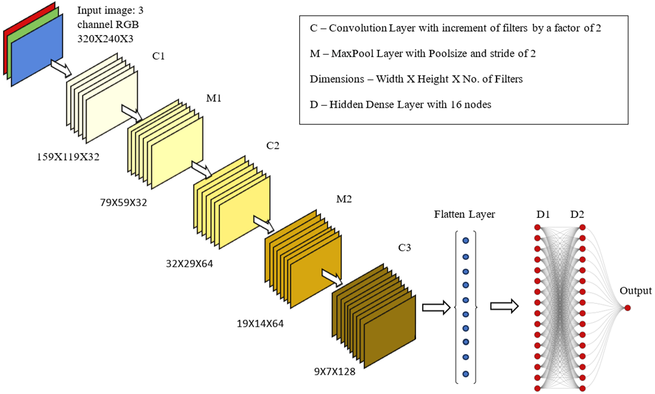
Figure 5: The proposed SegNet architecture specifically designed to be light on computations. This model can be deployed in drones with weak processing systems. The input image to this architecture is a segmented image achieved after segmentation of a complete $1280\times 720$ image into 12 smaller $320\times 240$ segments.

III-B SegNet Architecture

This algorithm is based on Convolution Neural Networks with Support Vector Machine used to draw a hyperplane among the data-points with ReLu classifier for convolutions [47, 48, 49, 50]. Successful use of linear support vector machines, for binary classification, was performed by many researchers [51, 48, 49, 52]. ReLu classifier has proven to be much faster at convergence compared to tanh and sigmoid [53]. The optimal hyperplane to separate two classes can be computed by the following set of equations [54].

$$f(w,x)=w.x+b$$ (1)

$$\text{min}\frac{1}{p}w^{\top}w+C\sum_{i=1}^{p}\text{max}(0,1-y_{i}(w^{t}x_{i}+b))^{2}$$ (2)

$w^{\top}w$ refers to the Manhattan norm (also known as $\mathcal{L}_{1}$ norm), $C$ denotes penalty parameter, $y_{i}$ denotes the actual label, and $w^{t}x_{i}+b$ denotes the predictor function. The differentiable counterpart, $\mathcal{L}_{2}$-SVM provides more stable results [6]

$$\text{min}\frac{1}{p}||w||_{2}^{2}+C\sum_{i=1}^{p}\text{max}(0,1-y_{i}(w^{t}x_{i}+b))^{2}$$ (3)

The model comprises of five layers of convolutions and two hidden layers separated by a flatten layer with one output layer that has a single dense node. These, in an order, are outlined in Table I.

TABLE I: SegNet architecture.

Layer	Description
1	1st Convolution 2D layer: Filters = 32, Activation function = ReLu, kernel size = $3\times 3$, Stride = 2, Input Shape = (240, 320, 3), padding = “SAME”
2	1st Maxpool layer: Pool Size = 2, Stride = 2
3	2nd Convolution 2D layer: Filters = 64, Activation function = ReLu, kernel size = $3\times 3$ , Stride = 2, padding = “SAME”
4	2nd Maxpool layer: Pool Size = 2, Stride = 2
5	3rd Convolution 2D layer: Filters = 128, Activation function = ReLu, kernel size = $3\times 3$, Stride = 2, padding = “SAME”
6	Flatten layer
7	1st Dense layer: Units = 16, Activation function = ReLu
8	2nd Dense layer: Units = 16, Activation function = ReLu
9	Output layer: Unit = 1, $\mathcal{L}_{2}$ regularization technique, Activation function = linear

IV Workflow, Challenges, and Mitigation

IV-A Overfitting Issue

During the initial algorithm tests, a concerning phenomenon emerged: the model exhibited signs of overfitting, where it excessively tailored itself to the training data. To address this issue, data augmentation techniques were implemented, intending to introduce variety into the dataset and curb overfitting. While these methods did alleviate the issue to some degree, they did not completely eradicate the problem. Additionally, attempts to mitigate overfitting through early stopping proved ineffective as the root cause was not solely over-training. A breakthrough came with the application of $\mathcal{L}_{2}$ regularization. This technique proved to be remarkably effective in addressing the overfitting challenge. $\mathcal{L}_{2}$ regularization operates by penalizing overly complex models, in particular in terms of weight values, effectively balancing the weights associated with different nodes in the neural network. By doing so, it corrected the bias present in the initial weight distribution, ensuring that no specific node dominated the others. This balance in weights significantly improved the model’s generalization abilities, allowing it to perform better on unseen data. The implementation of $\mathcal{L}_{2}$ regularization is pivotal during the training process. It not only highlights the bias issue within the model but also provides a viable solution by equalizing the influence of various nodes. This corrective measure significantly enhances the model’s ability to generalize, making it more reliable and effective in handling diverse datasets. Therefore, $\mathcal{L}_{2}$ regularization bolstering the overall robustness of the algorithm.

IV-B Workflow

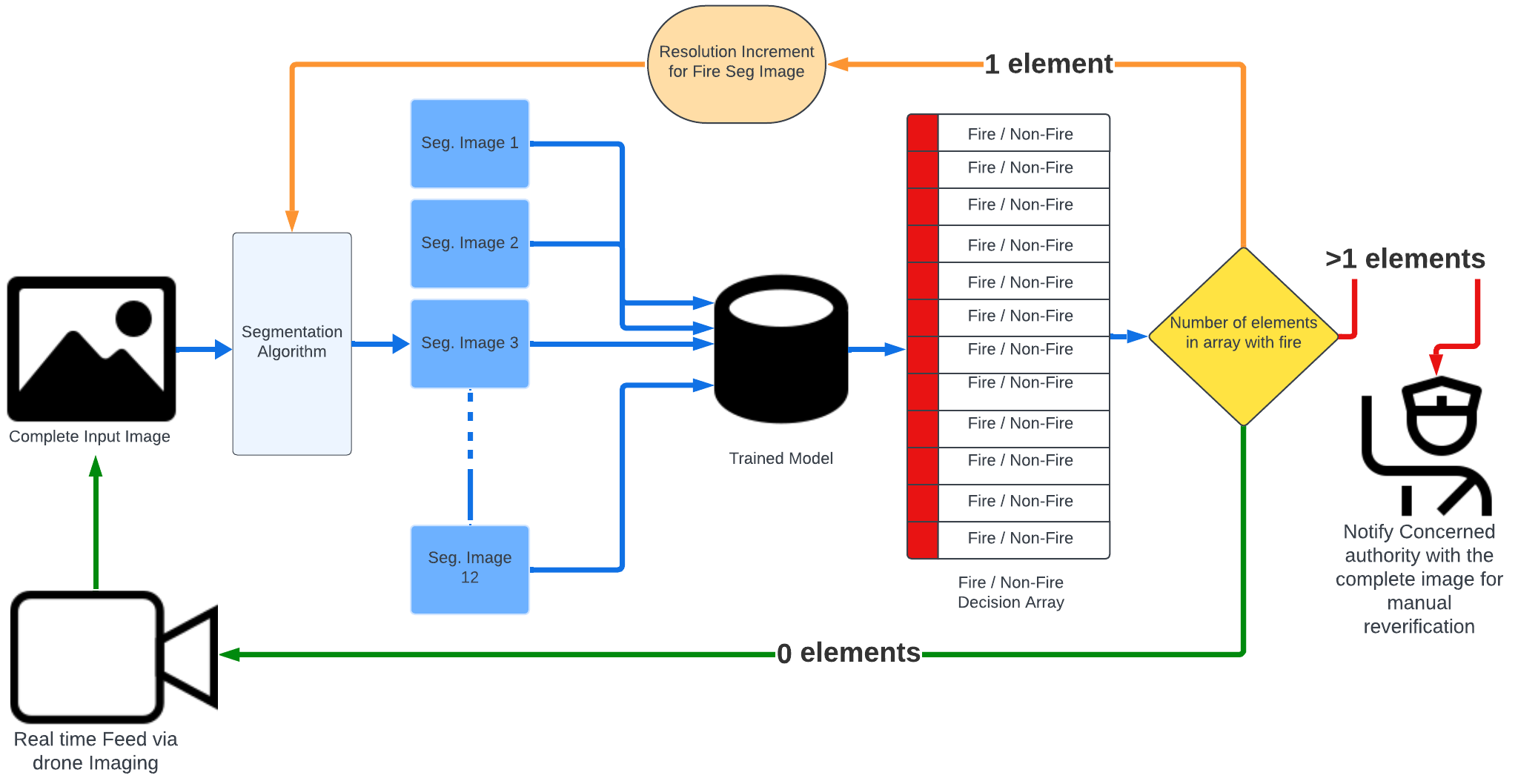
Figure 6: Workflow of a drone’s detection processing system with a model trained on the proposed SegNet architecture.

The development of this machine learning algorithm was meticulously designed with a specific workflow, as shown in Fig. 6, to achieve accurate classification results. At its core, the algorithm processes live video feed captured by drones, a crucial component in wildfire surveillance. The process begins by temporarily storing the video feed in the drone’s memory. This video stream is then divided into frames, with a specific subset of frames selected at fixed intervals, precisely one frame after every 19 frames in a 60 fps camera, translating to 3 frames per second. This intentional selection provides a buffer period, facilitated by the model’s swift processing speeds, allowing for additional secondary tasks to be executed. These tasks include intricate processes such as segmentation algorithms, real-time notifications to authorities upon fire detection, control of the drone’s flight systems, and integration with other sensors like GPS. One of the algorithm’s remarkable features is its ability to optimize resource utilization. By incorporating these secondary tasks within the main onboard processing unit, it eliminates the necessity for parallel processing units, reducing both the weight and production costs of surveillance drones significantly. This streamlined approach ensures the algorithm operates seamlessly within the drone’s existing framework, enhancing efficiency without compromising the drone’s overall functionality.

From an engineering perspective, this design choice not only minimizes the drone’s weight but also curtails production expenses, a critical factor given the need for deploying a substantial number of drones to cover vast forested areas effectively. The algorithm achieves this efficiency by employing a simple yet effective architecture. It utilizes a minimal number of convolution and dense layers, strategically balancing computational costs with high detection accuracy and rapid processing speeds. Upon receiving the segmented frames, depicted in Fig. 6, the algorithm proceeds to the segmentation stage. Each frame is dissected into 12 distinct segments, each maintaining a pixel size of $320\times 240$ without any loss of critical information. These individual segments are then fed into the machine learning model, meticulously trained for fire detection. The model’s output, whether it signifies the presence of fire or absence thereof, is stored in what is termed a "decision array" within the system. The decision array serves as a pivotal component in the algorithm’s decision-making process. If the array contains zero elements classified as fire, the algorithm accepts a new image from the live video feed storage, initiating a continuous cycle of assessment. When the array contains one element categorized as fire, the corresponding segmented image is reprocessed. Before reprocessing, this segment is rescaled to match the dimensions of a complete image. This step is fundamental in validating the initial classification, preventing potential false positives, and ensuring precision in the detection process. However, when the decision array reveals two or more elements marked as fire, the drone triggers a significant action. The complete image under examination is promptly forwarded to the relevant authorities for comprehensive verification and necessary further action. This approach ensures that potential wildfire incidents are promptly and accurately reported, allowing authorities to take swift and informed measures in response to the detected threat.

V Results

V-A SegNet Performance and Test Accuracy

The personal computing hardware used for building this model are: GPU – GTX 1660 TI MaxQ design (192-bit memory interface, 1.14 GHz clock speed), CPU – AMD Ryzen 9 4900HS (3 GHz clock speed, 7 nm process size), Software – Python 3.11.4, TensorFlow, Keras, numpy, PILLOW. An approach marked by caution was adopted, ensuring that enhancements were made conservatively to preserve the algorithm’s processing speed when it came to hyperparameter tuning and tuning the number of convolution and dense layers. Please follow this URL for video of the experiment.

TABLE II: Comprehensive performance analysis of the proposed SegNet: (a) Processing times of Segmented approach model with varying convolution and dense layers, and (b) Test accuracy of Segmented approach model with varying convolution and dense layers.

	SegNet number of convolution layers, time, and accuracy
	5 Conv	6 Conv	7 Conv	9 Conv	11 Conv
1 Dense	Low Acc	$389.32$ ms	$566$ ms	$812$ ms	Low Acc
Layer	$54.71\%$	$97.5\%$	$96.82\%$	$96.14\%$	$48.79\%$
2 Dense	$240.37$ ms	$1.34$ sec	$2.91$ sec	$3.32$ sec	Low Acc
Layer	$98.18\%$	$98.18\%$	$97.05\%$	$95.23\%$	$51.24\%$
3 Dense	$2.95$ sec	$4.06$ sec	$6.47$ sec	Low Acc	Low Acc
Layer	$97.95\%$	$97.7\%$	$94.78\%$	$72.56\%$	$39.31\%$

In the developmental stages of the model, depicted in Table II, various configurations of convolution layers (ranging from 5 to 11 layers) and dense layers (ranging from 1 to 3 layers) were systematically tested. Note that Conv is a short abbreviation denotes convolution. Prioritizing computational efficiency, a balance was sought between model speed and accuracy. Initial experiments with 5 convolution layers and 1 dense layer yielded a suboptimal accuracy of $54.71\%$, while an extensive configuration of 11 convolution layers and 3 dense layers resulted in a lower accuracy of $39.31\%$. The optimal compromise between accuracy and processing speed emerged with a configuration of 5 convolution layers and 2 dense layers, achieving an impressive $98.18\%$ accuracy and a processing time of $240.375$ ms. This careful exploration of model architecture during development ensures a harmonious blend of computational efficiency and accuracy in the proposed research.

TABLE III: SegNet imaging approaches.

	Dataset Categorization
	Original Complete Images	Augmented Complete Images	Segmented Images	Total
Fire	$5,195$	$547$	$2,266$	$5,968$
Non-Fire	$2,117$	$239$	$1,918$	$4,274$
Total	$7,312$	$786$	$2,144$	$10,242$

TABLE IV: SegNet different training consideration and enhancements.

	SegNet model accuracies with different training considerations and enhancements
	Simple Training	Early Stopping	Data Augmentation	$\mathcal{L}_{2}$-regularization
Training	$89.2\%$	$89.3\%$	$97.5\%$	$99.6\%$
Validation	$59.7\%$	$59.3\%$	$76.1\%$	$99.3\%$
Testing	$56.7\%$	$56.9\%$	$71.9\%$	$98.2\%$

Throughout the developmental phases, as shown in Table III and Table IV, the algorithm’s performance was carefully scrutinized, with model test accuracy being systematically recorded at each stage of improvement. Table III lists number of images in the training dataset including original images, augmented complete images, and segmented images for the case of fire and non-fire. Table IV illustrates accuracy improvements with different techniques to deal with overfitting. In its initial iteration, the model exhibited a $56.7\%$ accuracy, unmitigated by overfitting concerns. Notably, the training accuracy stood at $89.2\%$, while the validation accuracy was slightly higher at $59.7\%$ after 15 epochs. To counter overfitting, the first strategy employed was early stopping. However, this measure yielded results that were remarkably similar to the previous state, indicating that it did not substantially mitigate the overfitting issue. Subsequently, the integration of augmented images into the dataset emerged as the next step. This strategic addition led to a significant boost in training accuracy, elevating it to $97.5\%$, accompanied by a substantial rise in validation accuracy to $76.1\%$. Consequently, the model’s test accuracy, evaluated using a dataset comprising $441$ images, experienced a noteworthy increase from $56.7\%$ to $71.8\%$. Recognizing the need for a better solution, $\mathcal{L}_{2}$ norm regularization was implemented. This technique played a pivotal role in refining the model by adjusting weights and mitigating biases towards specific features. The impact was profound, evident in the substantial increase in training accuracy to $99.6\%$, with a corresponding validation accuracy of $99.3\%$. This adjustment resulted in a remarkable enhancement of the model’s test accuracy, reaching $98.2\%$. The cautious integration of techniques, from early stopping to augmented data, and finally, $\mathcal{L}_{2}$ norm regularization, resulted in a finely-tuned model. By addressing overfitting and refining its generalization capabilities, the algorithm achieved an accuracy rate that underlines its effectiveness and reliability, making it a potent tool in the realm of wildfire detection.

V-B Comparison Cutting Edge Techniques

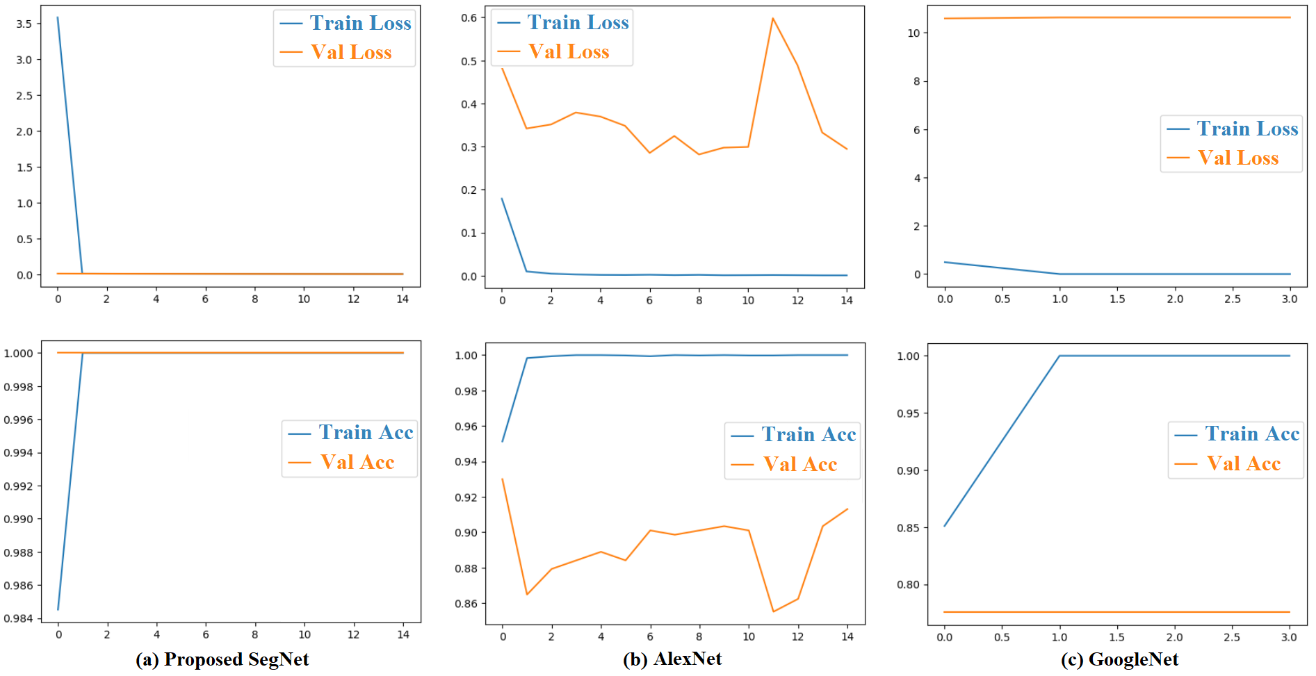
Figure 7: Comparison of Training/Validation accuracy and Losses to state-of-the-art literature: (a) Proposed SegNet, (b) AlexNet (literature), and (c) GoogleNet (literature).

To better understand the effectiveness of this proposed segmentation approach, the results are compared with state-of-the-art literature algorithms. These algorithms are GoogleNet [40] and AlexNet [41]. Both the algorithms were trained with the same dataset excluding the segmented images to help with proper comparison of results. Fig. 7.(a) shows the proposed SegNet performance, with train accuracy of $99.6\%$, validation accuracy of $99.3\%$, and test accuracy of $98.2\%$ with $0.0003$ train loss and validation loss of $0.0004$. Fig. 7.(b) presents AlexNet achieved model train accuracy of $100\%$, test accuracy of $92.2\%$, and validation accuracy of $91.3\%$ with 0.0005 training loss and $0.2943$ validation loss. Fig. 7.(c) depicts GoogleNet achieved model train accuracy of $99.9\%$, test accuracy of $76.8\%$ and validation accuracy of $77.5\%$. The recorded losses for training were $0.24$ and an increased loss $10.629$.

One of the main points of focus for this research was to reduce processing times along with the use of minimal computational power. Please visit Appendix A for comprehensive discussion about performance and time complexities. The processing speeds for proposed segmentation approach were observed and recorded at the stage of hyperparameter tuning and selection of number of convolution and dense layers. For the segmented approach single batch of 32 segmented images took an average of $641$ milliseconds.

$$\frac{641\text{ ms}}{32\text{ Seg Images}}=20.0312\frac{\text{ms}}{\text{Seg Images}}$$

A complete image consists of $12$ Segmented images:

$$20.0312\frac{\text{ms}}{\text{Seg Images}}\times 12=240.375\frac{\text{ms}}{\text{complete image}}$$

Thus, in the proposed segmented approach, a complete image of $1280\times 720$ pixel resolution was passed through the neural network within 240.37 milliseconds. The processing speeds of SegNet approach, GoogleNet and AlexNet were also compared for better understanding. As all the convolution layers are interconnected in GoogleNet in the form of inception block, which results in high number of computations, GoogleNet architecture was found to be the slowest with $1.487$ seconds. AlexNet performed better than GoogleNet as it was observed to be faster at $661.54$ milliseconds. The proposed SegNet was observed to be faster than both GoogleNet and AlexNet with $240.375$ milliseconds per complete image. The times mentioned are the average time observed for one complete image over 10 trials. As shown on Fig. 8, SegNet algorithm performs the best among the three models for each value of batch size. GoogleNet’s curve represents an incline in latency with increase in batch size. This is due to the interconnections of various different convolution blocks in the GoogleNet model architecture. Whereas, both AlexNet and SegNet perform with a curve close to linearity.

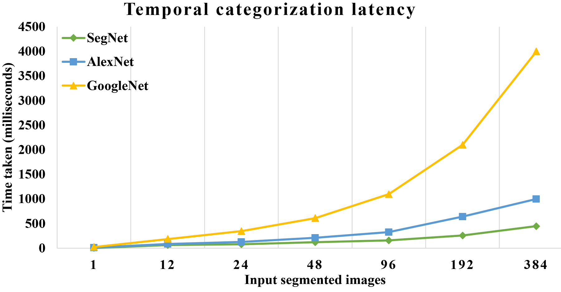
Figure 8: Temporal Categorization Latency chart: This chart represents the time required to perform classification task with different batch sizes of input images.

V-C SegNet Memory Requirements and Time Complexities

Memory requirements and time complexities calculations are detailed in Appendix A. The proposed SegNet architecture’s performance metrics are presented in Fig. 9.(a) and Fig. 9.(b) in terms of accuracy and precision rates. Fig. 9.(a) shows the number of images that were classified as one of the mentioned categories by SegNet on test data. Out of the selected 441 complete images for testing, 235 were categorized correctly as True Positives (TPs) and 198 were classified as True Negatives (TNs). This testifies to SegNet model’s effectiveness. As depicted, 5 False Positives (FPs) and 3 True Negatives signify the imperfections found in the model. With Accuracy of $98.18\%$ that exceeds results obtained by AlexNet and GoogleNet of $92.2\%$ and $76.8\%$ respectively. Fig 9.(b) shows the different performance metrics of SegNet. With a high recall, precision and accuracy, SegNet performs on par with most modern machine learning approaches, along with the model being computationally faster.

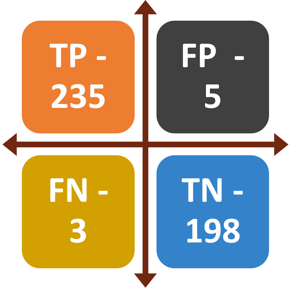
(a)

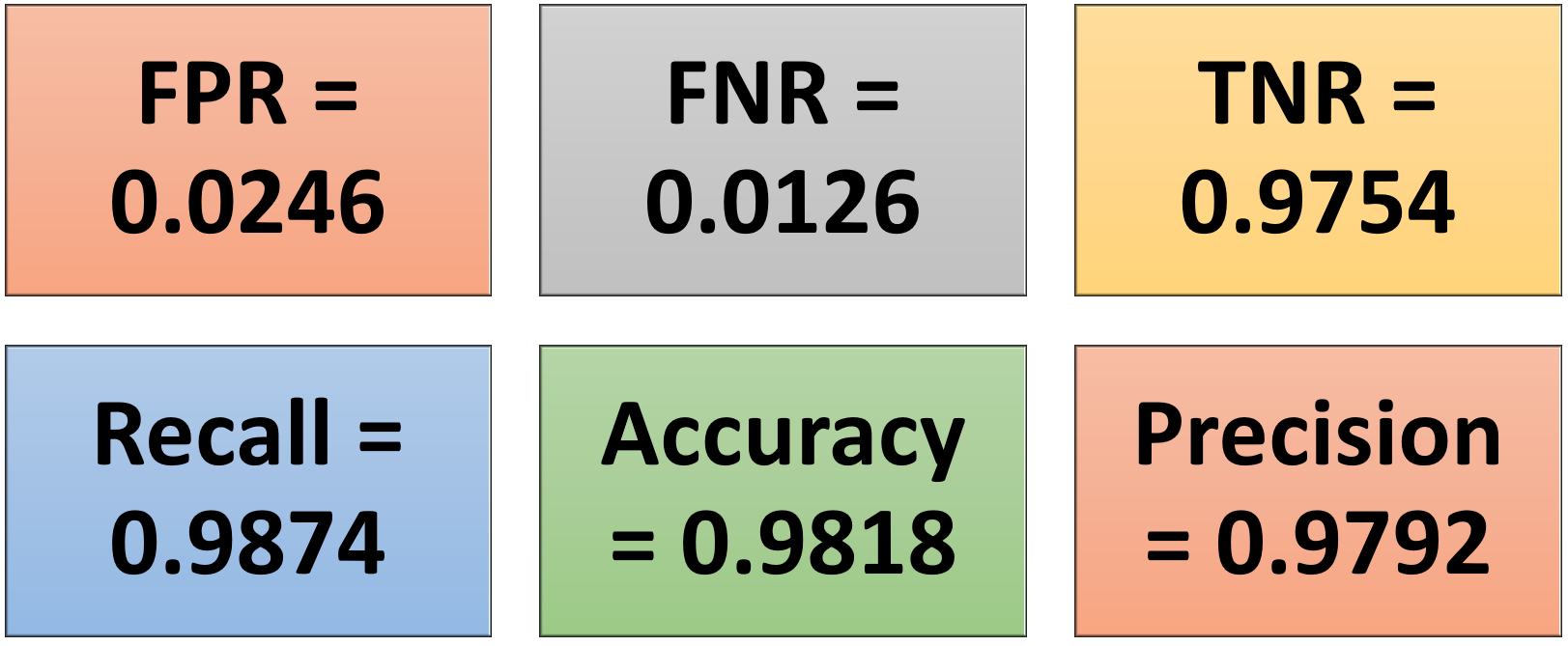
(b)

Figure 9: SegNet performance metric: (a) True Positive (TP), False Positive (FP), False Negative (FN), True Negative (TN); and (b) False Positive Rate (FPR), False Negative Rate (FNR), True Negative Rate (TNR), recall, accuracy and precision of the model.

Table V shows the memory consumption of the SegNet model. The SegNet model consumes 44.17 megabytes or 44,177,408 bytes of memory. Thus, any computational device on board a drone, with 50 megabytes of additional memory can perform operations of SegNet model. Table 6 also represents the total number of operations carried out for every layer. The total number of operations for SegNet model are 19.275 million. Thus, a drone with a processor with 19.275 MHz speed is required. For example, a common CPU on board drones manufactured by Qualcomm, the snapdragon 821 has the ability to perform at 2.15 GHz which could prove ideal for both the drone flight and wildfire detection algorithm’s processes. The data in Table V were collected using the expressions in Appendix A.

TABLE V: Metrics performance and the related mathematical formulas.

Layers	Parameters	Model space requirement (bytes)	Operational space requirement (bytes)	Total operations performed
Conv2D 1	896	7,168	2,889,856	8,242,560
MaxPool 1	-	-	-	-
Conv2D 1	18,496	147,968	1,322,752	4,095,360
MaxPool 1	-	-	-	-
Conv2D 1	73,856	590,848	636,544	2,021,760
Flatten	-	-	-	-
Dense 1	2,457,616	18,530,432	39,322,368	4,915,200
Dense 2	272	2,176	4,864	512
Output	17	136	1,024	32

VI Conclusion

In conclusion, this research addresses the critical challenges in wildfire detection, focusing on enhancing time resolution and optimizing processing speeds while maintaining high accuracy levels. Leveraging the power of Convolutional Neural Networks (CNNs), the study introduced a new approach: Segmented Neural Network (SegNet). This innovative method involved breaking down high-resolution images into smaller, manageable segments, allowing for rapid processing without compromising accuracy. The study meticulously navigated the complexities of feature reduction, acknowledging the inherent difficulties in balancing extensive feature maps with limited datasets. Through a systematic process, various techniques were applied to mitigate overfitting, enhance generalization, and achieve outstanding accuracy rates. Early stopping, data augmentation, and $\mathcal{L}_{2}$ norm regularization were sequentially implemented, each step refining the algorithm’s capabilities. The results demonstrated a significant leap in accuracy, with the final model achieving an impressive $98.2\%$ accuracy on the test dataset. A pivotal aspect of this research is the comparison with established algorithms, GoogleNet and AlexNet, which provided valuable insights. The segmentation approach outperformed these models, showcasing not only superior accuracy but also remarkable processing speeds. The segmentation technique processed a complete image of $1280\times 720$ pixels in just $240.37$ milliseconds, a testament to its efficiency in real-time applications. Beyond accuracy and speed, this research emphasized the importance of preserving essential details in images, especially in early wildfire detection scenarios. By ensuring the amorphous nature of fire, features were retained through segmentation, the algorithm excelled in detecting subtle signs of wildfire, crucial for timely intervention.

Furthermore, this research highlighted the algorithm’s integration within UAV drone systems. By optimizing resource utilization and minimizing computational costs, the algorithm can seamlessly integrate secondary tasks, such as real-time notifications, segmentation algorithms, and control systems, without the need for additional processing units. This streamlined approach significantly reduces production costs and drone weight, ensuring practicality and efficiency in real-world deployments. In summary, this research not only introduces a new segmentation approach for wildfire detection but also presents a comprehensive framework that balances accuracy, speed, and efficiency. By addressing critical challenges in real-time processing and detection accuracy, this study contributes significantly to the advancement of wildfire surveillance systems, promising enhanced safety and rapid response capabilities in the face of wildfire threats.

References

- [1] G. Zanchi and et al, “Simulation of water and chemical transport of chloride from the forest ecosystem to the stream,” Environmental Modelling & Software, vol. 138, p. 104984, 2021.
- [2] J. San-Miguel-Ayanz, J. M. Moreno, and A. Camia, “Analysis of large fires in european mediterranean landscapes: Lessons learned and perspectives,” Forest Ecology and Management, vol. 294, pp. 11–22, 2013.
- [3] Y. Wang and Y. Wu, “Scene classification with deep convolutional neural networks,” University of California, 2014.
- [4] J. MacCarthy, S. Tyukavina, M. Weisse, and N. Harris, “New data confirms: Forest fires are getting worse,” 2022.
- [5] M. C. Iban and A. Sekertekin, “Machine learning based wildfire susceptibility mapping using remotely sensed fire data and GIS: A case study of adana and mersin provinces, turkey,” Ecological Informatics, vol. 69, p. 101647, 2022.
- [6] A. M. Price-Whelan and et al, “The astropy project: building an open-science project and status of the v2. 0 core package,” The Astronomical Journal, vol. 156, no. 3, p. 123, 2018.
- [7] M. Filonchyk, M. P. Peterson, and D. Sun, “Deterioration of air quality associated with the 2020 us wildfires,” Science of The Total Environment, vol. 826, p. 154103, 2022.
- [8] A. L. Westerling, H. G. Hidalgo, D. R. Cayan, and T. W. Swetnam, “Warming and earlier spring increase western us forest wildfire activity,” science, vol. 313, no. 5789, pp. 940–943, 2006.
- [9] P. Hawken, “Regeneration: Ending the climate crisis in one generation,” Penguin, vol. 1, 2021.
- [10] H. A. Hashim, A. E. Eltoukhy, and K. G. Vamvoudakis, “Uwb ranging and imu data fusion: Overview and nonlinear stochastic filter for inertial navigation,” IEEE Transactions on Intelligent Transportation Systems, vol. 25, no. 1, pp. 359–369, 2024.
- [11] H. A. Hashim, M. Abouheaf, and M. A. Abido, “Geometric stochastic filter with guaranteed performance for autonomous navigation based on imu and feature sensor fusion,” Control Engineering Practice, vol. 116, p. 104926, 2021.
- [12] H. A. Hashim and A. E. Eltoukhy, “Landmark and imu data fusion: Systematic convergence geometric nonlinear observer for slam and velocity bias,” IEEE Transactions on Intelligent Transportation Systems, vol. 23, no. 4, pp. 3292–3301, 2022.
- [13] A. Gaur and et al, “Fire sensing technologies: A review,” IEEE Sensors Journal, vol. 19, no. 9, pp. 3191–3202, 2019.
- [14] P. Barmpoutis, P. Papaioannou, K. Dimitropoulos, and N. Grammalidis, “A review on early forest fire detection systems using optical remote sensing,” Sensors, vol. 20, no. 22, p. 6442, 2020.
- [15] R. Ghali, M. A. Akhloufi, and W. S. Mseddi, “Deep learning and transformer approaches for UAV-based wildfire detection and segmentation,” Sensors, vol. 22, no. 5, p. 1977, 2022.
- [16] T. Vishwanath, R. D. Shirwaikar, W. M. Jaiswal, and M. Yashaswini, “Social media data extraction for disaster management aid using deep learning techniques,” Remote Sensing Applications: Society and Environment, vol. 30, p. 100961, 2023.
- [17] O. M. Bushnaq, A. Chaaban, and T. Y. Al-Naffouri, “The role of UAV-IoT networks in future wildfire detection,” IEEE Internet of Things Journal, vol. 8, no. 23, pp. 16 984–16 999, 2021.
- [18] H. A. Hashim, “Exponentially stable observer-based controller for vtol-uavs without velocity measurements,” International Journal of Control, vol. 96, no. 8, pp. 1946–1960, 2023.
- [19] H. A. Hashim, A. E. Eltoukhy, and A. Odry, “Observer-based controller for vtol-uavs tracking using direct vision-aided inertial navigation measurements,” ISA transactions, vol. 137, pp. 133–143, 2023.
- [20] C. Yuan, Z. Liu, and Y. Zhang, “Fire detection using infrared images for UAV-based forest fire surveillance,” in 2017 International Conference on Unmanned Aircraft Systems (ICUAS). IEEE, 2017, pp. 567–572.
- [21] M. A. Akhloufi, A. Couturier, and N. A. Castro, “Unmanned aerial vehicles for wildland fires: Sensing, perception, cooperation and assistance,” Drones, vol. 5, no. 1, p. 15, 2021.
- [22] S. Albawi, T. A. Mohammed, and S. Al-Zawi, “Understanding of a convolutional neural network,” in 2017 international conference on engineering and technology (ICET). Ieee, 2017, pp. 1–6.
- [23] K. A. Ghamry and Y. Zhang, “Cooperative control of multiple UAVs for forest fire monitoring and detection,” in 2016 12th IEEE/ASME International Conference on Mechatronic and Embedded Systems and Applications (MESA). IEEE, 2016, pp. 1–6.
- [24] T. Giitsidis, E. G. Karakasis, A. Gasteratos, and G. C. Sirakoulis, “Human and fire detection from high altitude UAV images,” in 2015 23rd Euromicro international conference on parallel, distributed, and network-based processing. IEEE, 2015, pp. 309–315.
- [25] Q. Hu, X. Wei, X. Liang, L. Zhou, W. He, Y. Chang, Q. Zhang, C. Li, and X. Wu, “In-process vision monitoring methods for aircraft coating laser cleaning based on deep learning,” Optics and Lasers in Engineering, vol. 160, p. 107291, 2023.
- [26] Z. Jiao, Y. Zhang, J. Xin, L. Mu, Y. Yi, H. Liu, and D. Liu, “A deep learning based forest fire detection approach using UAV and YOLOv3,” in 2019 1st International conference on industrial artificial intelligence (IAI). IEEE, 2019, pp. 1–5.
- [27] F. Huot and et al, “Deep learning models for predicting wildfires from historical remote-sensing data,” arXiv preprint arXiv:2010.07445, vol. 1, pp. 1–10, 2020.
- [28] S. Shao, P. Wang, and R. Yan, “Generative adversarial networks for data augmentation in machine fault diagnosis,” vol. 106. Computers in Industry, Elsevier, 2019, pp. 85–93.
- [29] A. Bochkovskiy, C.-Y. Wang, and H.-Y. M. Liao, “Yolov4: Optimal speed and accuracy of object detection,” arXiv preprint arXiv:2004.10934, vol. 1, pp. 1–10, 2020.
- [30] S. Ren, K. He, R. Girshick, and J. Sun, “Faster r-CNN: Towards real-time object detection with region proposal networks,” Advances in neural information processing systems, vol. 28, 2015.
- [31] E. Pena-Molina and et al., “Postfire damage zoning with open low-density lidar data sources in semi-arid forests of the iberian peninsula,” Remote Sensing Applications: Society and Environment, p. 101114, 2023.
- [32] M. Alkhaleefah and C.-C. Wu, “A hybrid CNN and RBF-based SVM approach for breast cancer classification in mammograms,” in 2018 IEEE International Conference on Systems, Man, and Cybernetics (SMC). IEEE, 2018, pp. 894–899.
- [33] V. L. Arruda and et al., “An alternative approach for mapping burn scars using landsat imagery, google earth engine, and deep learning in the brazilian savanna,” Remote Sensing Applications: Society and Environment, vol. 22, p. 100472, 2021.
- [34] N. N. Thach and et al, “Spatial pattern assessment of tropical forest fire danger at thuan chau area (vietnam) using GIS-based advanced machine learning algorithms: A comparative study,” Ecological Informatics, vol. 46, pp. 74–85, 2018.
- [35] A. Bjanes, R. De La Fuente, and P. Mena, “A deep learning ensemble model for wildfire susceptibility mapping,” Ecological Informatics, vol. 65, p. 101397, 2021.
- [36] S. Yousefi and et al, “A machine learning framework for multi-hazards modeling and mapping in a mountainous area,” Scientific Reports, vol. 10, no. 1, p. 12144, 2020.
- [37] S. Eskandari, H. R. Pourghasemi, and J. P. Tiefenbacher, “Fire-susceptibility mapping in the natural areas of iran using new and ensemble data-mining models,” Environmental Science and Pollution Research, vol. 28, no. 34, pp. 47 395–47 406, 2021.
- [38] S. Treneska and B. R. Stojkoska, “Wildfire detection from UAV collected images using transfer learning,” in Proceedings of the 18th International Conference on Informatics and Information Technologies, Skopje, North Macedonia, 2021, pp. 6–7.
- [39] F. Zhu, H. Li, W. Ouyang, N. Yu, and X. Wang, “Learning spatial regularization with image-level supervisions for multi-label image classification,” in Proceedings of the IEEE conference on computer vision and pattern recognition, 2017, pp. 5513–5522.
- [40] F. Yuesheng and et al, “Circular fruit and vegetable classification based on optimized GoogleNet,” IEEE Access, vol. 9, pp. 113 599–113 611, 2021.
- [41] A. Bouguettaya, H. Zarzour, A. M. Taberkit, and A. Kechida, “A review on early wildfire detection from unmanned aerial vehicles using deep learning-based computer vision algorithms,” Signal Processing, vol. 190, p. 108309, 2022.
- [42] C. Acosta, “Drone footage of white mountains foliage will blow your mind,” 2023. [Online]. Available: https://wokq.com/drone-footage-of-white-mountains-foliage-will-blow-your-mind/
- [43] P. Jeatrakul, K. W. Wong, and C. C. Fung, “Data cleaning for classification using misclassification analysis.” Journal of Advanced Computational Intelligence and Intelligent Informatics, vol. 14, no. 3, pp. 297–302, 2010.
- [44] Y.-S. Wang, C.-L. Tai, O. Sorkine, and T.-Y. Lee, “Optimized scale-and-stretch for image resizing,” in ACM SIGGRAPH Asia 2008 papers, 2008, pp. 1–8.
- [45] Y. Guan, F. Zhou, and J. Zhou, “Research and practice of image processing based on python,” in Journal of Physics: Conference Series, vol. 1345, no. 2. IOP Publishing, 2019, p. 022018.
- [46] P. Kim, “Matlab deep learning,” With machine learning, neural networks and artificial intelligence, vol. 130, no. 21, 2017.
- [47] A. F. Agarap, “An architecture combining convolutional neural network (CNN) and support vector machine (SVM) for image classification,” arXiv preprint arXiv:1712.03541, vol. 1, pp. 1–10, 2017.
- [48] C. Cortes and V. Vapnik, “Support-vector networks,” Machine Learning, vol. 20, pp. 273–297, 1995.
- [49] P. Kamavisdar, S. Saluja, S. Agrawal et al., “A survey on image classification approaches and techniques,” International Journal of Advanced Research in Computer and Communication Engineering, vol. 2, no. 1, pp. 1005–1009, 2013.
- [50] A. Krizhevsky, I. Sutskever, and G. E. Hinton, “Imagenet classification with deep convolutional neural networks,” Advances in neural information processing systems, vol. 25, 2012.
- [51] S. Y. Chaganti and et al, “Image classification using SVM and CNN,” in 2020 International Conference on Computer Science, Engineering and Applications (ICCSEA). IEEE, 2020, pp. 1–5.
- [52] Y. Tang, “Deep learning using linear support vector machines,” arXiv preprint arXiv:1306.0239, 2013.
- [53] R. H. Hahnloser, R. Sarpeshkar, M. A. Mahowald, R. J. Douglas, and H. S. Seung, “Digital selection and analogue amplification coexist in a cortex-inspired silicon circuit,” nature, vol. 405, no. 6789, pp. 947–951, 2000.
- [54] M. Wauters and M. Vanhoucke, “Support vector machine regression for project control forecasting,” vol. 47. Automation in Construction, Elsevier, 2014, pp. 92–106.
- [55] G. J. Woeginger, “Space and time complexity of exact algorithms: Some open problems,” in International Workshop on Parameterized and Exact Computation. Springer, 2004, pp. 281–290.
- [56] Y. Gao and J. Culberson, “Space complexity of estimation of distribution algorithms,” Evolutionary Computation, vol. 13, no. 1, pp. 125–143, 2005.
- [57] C. H. Papadimitriou, “Computational complexity,” in Encyclopedia of computer science, 2003, pp. 260–265.