Multidimensional Compressed Sensing for Spectral Light Field Imaging

Abstract

This paper considers a compressive multi-spectral light field camera model that utilizes a one-hot spectral-coded mask and a microlens array to capture spatial, angular, and spectral information using a single monochrome sensor. We propose a model that employs compressed sensing techniques to reconstruct the complete multi-spectral light field from undersampled measurements. Unlike previous work where a light field is vectorized to a 1D signal, our method employs a 5D basis and a novel 5D measurement model, hence, matching the intrinsic dimensionality of multispectral light fields. We mathematically and empirically show the equivalence of 5D and 1D sensing models, and most importantly that the 5D framework achieves orders of magnitude faster reconstruction while requiring a small fraction of the memory. Moreover, our new multidimensional sensing model opens new research directions for designing efficient visual data acquisition algorithms and hardware.

1 INTRODUCTION

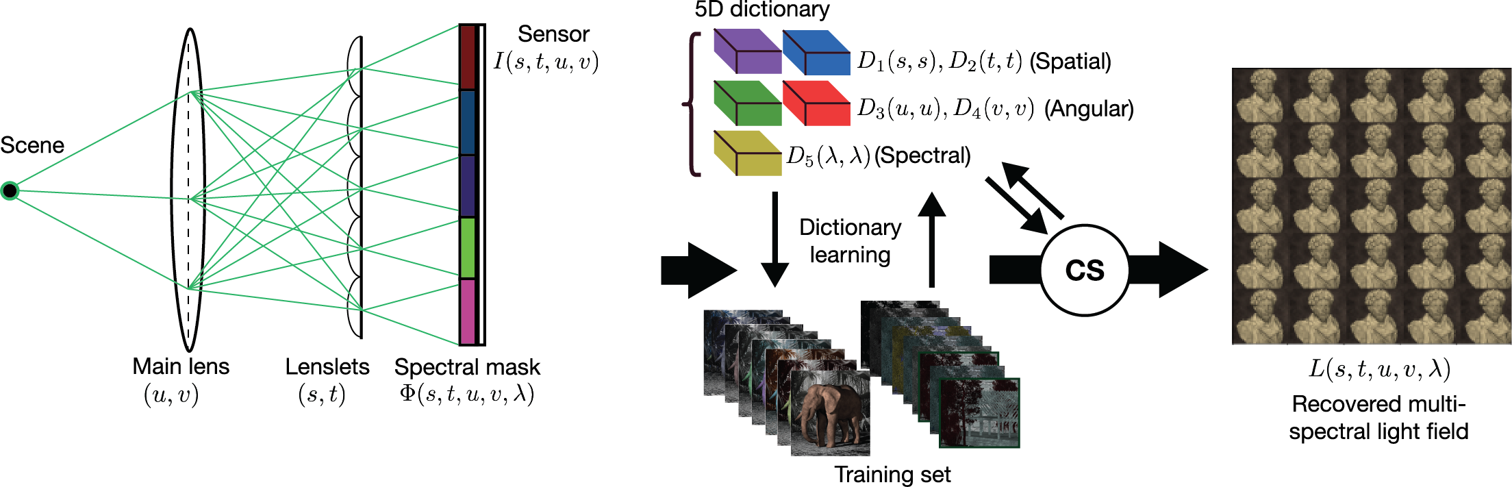
Figure 1: Illustrates the proposed compressed sensing framework for multi-spectral light field capture and reconstruction. Compressed light fields are captured using a lenslet array placed in the optical path and a one-hot spectral CFA mask placed on the sensor. Our proposed $nD$ compressed sensing formulation improves the reconstruction time by orders of magnitude as compared to the commonly used 1D compressed sensing techniques without any quality degradation.

Computational cameras for light field capture, [Levoy and Hanrahan, 1996, Gortler et al., 1996], post capture editing and scene analysis have become increasingly popular and found applications ranging from photography and computer vision to capture of neural radiance fields. Light field imaging aims to obtain multidimensional optical information including spatial, angular, spectral, and temporal sampling of the scene. Inherent to most light field capture systems is the trade-off between the complexity and cost of the acquisition system and the output image quality in terms of spatial and angular resolution. On one hand camera arrays, [Wilburn et al., 2005], offer high resolution but comes with high cost and complex bulky mechanical setups, while systems based on microlens, or lenslet, arrays placed in the optical path, [Ng et al., 2005], sacrifices resolution for the benefit of light weight systems and lower costs.

A key goal in the development of next generation light field imaging systems is to enable high quality multispectral measurements of complex scenes based on a minimum amount of input measurements. Focusing on cameras with lenslet arrays, such optical systems capture 2D projections of the full 5D (spatial, angular, spectral) light field image data. Reconstruction of the high dimensional 5D data from the 2D measurements is challenging, due to the dimensionality gap and high compression ratio resulting from undersampling of, e.g., the spectral domain. Compressed sensing (CS) has emerged as a popular approach for light field reconstruction, however, current systems are either not designed for multispectral reconstruction, [Marwah et al., 2013, Miandji et al., 2019], and/or fundamentally rely on 1D CS reconstruction, [Marquez et al., 2020], disregarding the original signal dimensionality. Since a light field is fundamentally a 5D object, a vectorized 1D representation of such data will prohibit the exploitation of data coherence along each dimension, which has been observed in a number of previous works on sparse representation of multidimensional data [Miandji et al., 2019]. Another problem with 1D reconstruction is that it inherently leads to prohibitively large storage costs for the dictionary and sensing matrices as well as long reconstruction times.

In this paper, we formulate the light field capture and reconstruction as a multidimensional, $nD$, compressed sensing problem. As a first step, see Fig. 1, we learn a 5D dictionary ensemble [Miandji et al., 2019] from the spatial (2D), angular (2D), and spectral (1D) domains of a light field training set. Using a novel 5D sensing model based on a one-hot sampling pattern (implemented as a multispectral color filter array (CFA) on the sensor), we obtain measurements of a light field in the test set. The 5D sensing model is composed of 5 measurement matrices, each corresponding to one dimension of the light field. By randomizing the one-hot measurement for each measurement matrix, we promote the incoherence of the measurement matrices with respect to the 5D dictionary. The one-hot spectral sampling mask allows us to design a spectral light field camera with a monochrome sensor. Another advantage of the one-hot mask is cost-effectiveness, since it has a similar manufacturing complexity compared to a Color Filter Array (CFA), which is commonly used in consumer-level digital cameras. Finally, we extend the Smoothed-$\ell_{0}$ (SL0) method for 2D signals [Ghaffari et al., 2009] to 5D signals, enabling fast reconstructions of the light field from the measurements without the need for manipulating the dimensionality of the light field.

The main contributions are:

• A novel $nD$ formulation for a single sensor compressive spectral light field camera design, where a one-hot sensing model together with a learned multidimensional sparse representation is utilized.

• An $nD$ recovery method that is more than two orders of magnitude faster than the widely used 1D formulation and recovery.

• We show, both theoretically and experimentally, that the $n$D formulation is far superior to the $1$D variant both in terms of memory and speed.

Our sensing model derivation shows that the $n$D sensing is mathematically equivalent to 1D sensing with the same number of samples. Experimental results confirm such equivalence in terms of reconstruction quality. Most importantly, the evaluations show that the proposed novel formulation produces high quality results orders of magnitude faster compared to methods based on 1D compressed sensing. Our multidimensional sensing model opens up flexible sensing mask designs where each dimension can be treated individually.

2 RELATED WORK

Common approaches for light field imaging include the use of coded apertures [Liang et al., 2008, Babacan et al., 2009] and lenslet arrays [Ng et al., 2005], and more recently combinations of the two [Marquez et al., 2020]. Combining compressive sensing with spectrometers, coded aperture snapshot spectral imagers are also known as compressive spectral imagers (CASSI). In general, a CASSI system consists of a coded mask, prisms, and an imaging sensor. Examples of capture systems are for example described by [Hua et al., 2022], and [Xiong et al., 2017]. Based on the detector measurements and the coded mask information the final spectral images or light fields are then typically reconstructed using compressed sensing methods [Arce et al., 2014, Marquez et al., 2020, Yuan et al., 2021]. Recently, deep learning based methods have shown promising results for the application of multispectral image reconstruction, for an overview, see the survey by [Huang et al., 2022]. Related to our approach [Schambach et al., 2021] proposed a multi-task deep learning method to estimate the center view and depth from the coded measurements. The approach yields good results, but is not directly comparable to our approach since the aim here is to recover the full 5D light field and not a depth map.

Compared to previous work, our $nD$ formulation presents several benefits such as flexible design of the 5D light field sensing masks as well as orders of magnitude speed up without any quality degradation as compared to the 1D sensing used in previous work. One of the key insights, and contributions, enabling the $nD$ CS framework is the sensing mask formulation illustrated in Fig. 2, where the Kronecker product of a set of small design matrices lead to the one-hot CFA mask used for $nD$ compressed sampling. This as well as our general formulation are described in detail in the next section.

3 Multidimensional Compressive Light Fields

Our capture system, see Fig. 1, records a set of angular views as produced by the lenslet array, where a one-hot spectral coded mask at the resolution of the lenslet is placed on the sensor. In the design, we assume that there are $n$ different types of filters with different spectral characteristics available, and that the goal is to formulate a one-hot coded mask such that each measurement, or pixel on the sensor, integrates the incoming light rays modulated by one of the $n$ different filter types. This is motivated by the fact that we want to enable capture of a well defined set of spectral bands, typically defined by the imaging application.

3.1 The measurement model

Our camera design measures the spatial and angular information, while the spectral information, due to the one-hot mask, is compressed to a single value. Let $L(s,t,u,v,\lambda)$ represent the light field function following the commonly used two-plane parameterization, where $(s,t)$ and $(u,v)$ denotes the spatial and angular dimensions, and $\lambda$ the spectral dimension. Moreover, let $I(s,t,u,v)$ be the compressed measurements recorded by the sensor. We formulate the multispectral compressive imaging pipeline as follows

$$I(s,t,\mu,\nu)=\int_{\lambda}\Phi(s,t,u,v,\lambda)L(s,t,u,v,\lambda)\text{d}\lambda,$$ (1)

where $\Phi(s,t,u,v,\lambda)$ is the 5D sensing operator, as shown in Fig. 2. Specifically, due to our design of the one-hot binary mask, we have

$$\sum_{\lambda=1}^{n}\Phi[s,t,u,v,\lambda]=1,$$ (2)

making sure that only one spectral channel is sampled for every pixel on the monochrome sensor.

According to (1), our goal is to recover the full multispectral light field $L$ from its measurements $I$ and with the knowledge of the measurement operator $\Phi$ constructed from the one-hot mask. Indeed, since (1) is a linear measurement model, we can rewrite it as $I=\Phi L$, where $L$ is the light field arranged in a vector and $\Phi$ is the measurement matrix. In this case, recovering $L$ amounts to solving an underdetermined system of linear equations, which is a topic addressed by compressed sensing [Candes and Wakin, 2008].

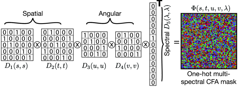
Figure 2: Illustration of Kronecker-based coded attenuation masks.

3.2 Compressed sensing

The underdetermined system of linear equations $I=\Phi L$ can be solved by regularizing the problem based on sparsity of the light field in a suitable basis or dictionary $D$ as follows

$$\vspace{-3pt}\mathop{argmin}\limits_{\alpha}{\|\alpha\|_{0}}\quad\textrm{s.t.}\quad||{I}-\Phi D\alpha||_{2}\leq\epsilon,\vspace{-3pt}$$ (3)

where $\epsilon$ is a user-defined threshold for the data fidelity and $\|.\|_{0}$ denotes the $\ell_{0}$ pseudo-norm. The dictionary $D$ can be obtained from analytical basis function, e.g., Discrete Cosine Transform (DCT), or by training-based algorithms, e.g., K-SVD [Aharon et al., 2006]. Equation (3) can be solved by several algorithms and in this paper we use Smoothed-$\ell_{0}$ (SL0) [Mohimani et al., 2010]. We note that (3) solves a 1D compressed sensing problem, and therefore utilizes a 1D dictionary. As mentioned, our goal is to solve (3) using multidimensional dictionaries and a multidimensional sensing model.

3.3 Learning-based multidimensional dictionary

To this end, we utilize the Aggregated Multidimensional Dictionary Ensemble (AMDE) [Miandji et al., 2019] to train an ensemble of 5D orthogonal dictionaries to efficiently represent spatial, angular, and spectral dimensions of a light field. In particular, we have $D_{1}\in\mathbb{R}^{s\times s},D_{2}\in\mathbb{R}^{t\times t},D_{3}\in\mathbb{R}^{u\times u},D_{4}\in\mathbb{R}^{v\times v},D_{5}\in\mathbb{R}^{\lambda\times\lambda}$. The 1D dictionary, used in (3), can be obtained from a 5D dictionary using the Kronecker product [Duarte and Baraniuk, 2012] as follows

$$D=D_{5}\otimes D_{4}\otimes D_{3}\otimes D_{2}\otimes D_{1},$$ (4)

where $D\in\mathbb{R}^{stuv\lambda\times stuv\lambda}$. Indeed, the storage cost of $D$ is prohibitively large compared to the per-dimension dictionaries $D_{i}$. The memory requirement ratio between a 1D and a 5D dictionary is $\frac{(stuv\lambda)^{2}}{s^{2}+t^{2}+u^{2}+v^{2}+\lambda^{2}}$. This further motivates a multidimensional dictionary and sensing model.

3.4 Multidimensional measurement model

In multidimensional sensing, a requirement is to introduce a separate sensing operator for each dimension of the signal. Since a light field is 5D, we need to design 5 sensing operators to obtain measurements from the spatial, angular, and spectral domains. Let $\Phi_{j}$, $j=1,\dots,5$ be the set of sensing matrices (or operators) for a 5D light field. Utilizing the n-mode product between a tensor and a matrix [Kolda and Bader, 2009], we can formulate the multidimensional measurement model as follows

$$\vspace{-0pt}\bm{\mathcal{I}}=\bm{\mathcal{L}}\times_{1}\Phi_{1}\times_{2}\Phi_{2}\times_{3}\Phi_{3}\times_{4}\Phi_{4}\times_{5}\Phi_{5}\vspace{-0pt}$$ (5)

where $\bm{\mathcal{L}}\in\mathbb{R}^{s\times t\times u\times v\times\lambda}$ is the light field tensor and $\bm{\mathcal{I}}\in\mathbb{R}^{s\times t\times u\times v}$ is the compressed measurements on the sensor. The choice of sensing matrices $\Phi_{j}$ is of utmost importance in any compressive acquisition setup. Due to our camera design in Fig. 1, i.e. the use of a lenslet array, we do not perform compression on spatial and angular domains. As a result, $\Phi_{j}$, $j=1,\dots,4$, are identity matrices. However, we would like to maximize the incoherence between the dictionary and the sensing matrices [Candes and Wakin, 2008]. Therefore, as illustrated in Fig. 2, we perform a random row-shuffling of the identity matrices to form $\Phi_{j}$, $j=1,\dots,4$. On the other hand, since we perform spectral compression using the one-hot mask, $\Phi_{5}\in\mathbb{R}^{1\times n}$ contains only one nonzero value, where $n$ is the total number of spectral bands. In our experiments, we used data sets where $n=13$.

The multidimensional measurement model in (5) can be converted to a 1D measurement model as follows

$$I=\underbrace{(\Phi_{5}\otimes\Phi_{4}\otimes\Phi_{3}\otimes\Phi_{2}\otimes\Phi_{1})}_{\Phi}L,\vspace{-3pt}$$ (6)

where L and I are vectorized forms of the tensors $\bm{\mathcal{L}}$ and $\bm{\mathcal{I}}$, respectively. An illustration of the Kronecker product of sensing matrices $\Phi_{j}$ is shown in Fig. 2. Note that the key benefit of the nD sensing model is that it requires several orders of magnitude less memory compared to the Kronecker 1D sensing model in (6). Recall from Section 3.3 that our 5D AMDE dictionary also exhibits such benefits. The nD approach also comes with the benefit that the sensing mask can be designed using only five small matrices.

The pseudocode in Algorithm 1 illustrates nD SL0 reconstruction given the measurements $\bm{\mathcal{I}}$ and the matrices $\mathbf{A}^{(i)}=\Phi_{i}D_{i}$ as presented in Section 3.5.

Algorithm 1 Multidimensional SL0 algorithm

0:  Input tensor $\bm{\mathcal{I}}$, input matrices $\mathbf{A}^{(1\ldots n)}$, limit parameter $\sigma_{min}$, decreasing factor $\sigma_{f}$, iteration $L$, step $\mu$

0:  $\bm{\mathcal{S}}$ as sparse solution of $\bm{\mathcal{S}}\times_{1\ldots n}\mathbf{A}^{(1\ldots n)}=\bm{\mathcal{I}}$

1:  $\bm{\mathcal{S}}\leftarrow\bm{\mathcal{I}}\times_{1\ldots n}\mathbf{A}^{(1\ldots n)\dagger}$   {initial estimate, $\dagger$ denotes pseudo-inverse}

2:  $\sigma\leftarrow$ largest absolute element of $\bm{\mathcal{I}}$

3:  while $\sigma>\sigma_{min}$ do

4:     for $k=1\ldots L$ do

5:        $\Delta\bm{\mathcal{S}}=-\frac{\bm{\mathcal{S}}}{\sigma^{2}}\circ exp\Big{(}-\frac{\bm{\mathcal{S}}\circ\bm{\mathcal{S}}}{2\sigma^{2}}\Big{)}$

6:        $\hat{\bm{\mathcal{S}}}\leftarrow\mu\cdot\Delta\bm{\mathcal{S}}$   {Steepest ascent step}

7:        $\hat{\bm{\mathcal{S}}}\leftarrow\hat{\bm{\mathcal{S}}}-(\hat{\bm{\mathcal{S}}}\times_{1\ldots n}\mathbf{A}^{(1\ldots n)}-\bm{\mathcal{I}})\times_{1\ldots n}\mathbf{A}^{(1\ldots n)\dagger}$

8:     end for

9:     $\bm{\mathcal{S}}\leftarrow\hat{\bm{\mathcal{S}}}$

10:     $\sigma=\sigma_{f}\cdot\sigma$

11:  end while

3.5 Reconstruction

Given the AMDE dictionary in Section 3.3 and the multidimensional measurement model in Section 3.4, we formulate the 5D light field recovery algorithm from its measurements as follows

$$\vspace{-5pt}\mathop{argmin}\limits_{\bm{\mathcal{S}}}\|\bm{\mathcal{S}}\|_{0}\quad\textrm{s.t.}\quad\|\bm{\mathcal{I}}-\bm{\mathcal{S}}\times_{1}\Phi_{1}D_{1}\times_{2}\Phi_{2}D_{2}\times_{3}\\ \Phi_{3}D_{3}\times_{4}\Phi_{4}D_{4}\times_{5}\Phi_{5}D_{5}\|_{2}\leq\epsilon,\vspace{-5pt}$$ (7)

where $\bm{\mathcal{S}}\in\mathbb{R}^{s\times t\times u\times v\times\lambda}$ is a sparse coefficient vector. Once the coefficients are obtained, the full light field is computed as $\hat{\bm{\mathcal{L}}}=\bm{\mathcal{S}}\times_{1}D_{1}\times_{2}D_{2}\times_{3}D_{3}\times_{4}D_{4}\times_{5}D_{5}$. To solve (7), we extend the 2D SL0 algorithm [Ghaffari et al., 2009] for higher dimensional signals. A pseudo-code of the 5D SL0 algorithm is provided in Algorithm 1.

4 Evaluation and results

Table 1: Comparing 5D DCT, 1D AMDE and 5D AMDE using five test spectral light fields under ONE snapshot. Proposed Method in blue. Best values in bold.

Test	Methods	PSNR /dB		SSIM			SA/(∘)
Scenes	5D	1D	5D	5D	1D	5D	5D	1D	5D
	DCT	AMDE	AMDE	DCT	AMDE	AMDE	DCT	AMDE	AMDE
Bust	25.388	31.944	31.944	0.741	0.812	0.812	22.6658	10.853	10.853
Cabin	15.798	20.275	20.2754	0.302	0.636	0.636	53.767	26.977	26.977
Circles	15.459	18.494	18.494	0.313	0.530	0.530	35.216	29.588	29.588
Dots	15.454	23.485	23.485	0.247	0.738	0.738	24.661	10.668	10.668
Elephants	18.108	24.880	24.880	0.5761	0.743	0.7435	23.161	17.356	17.356
Average	14.631	22.398	22.398	0.324	0.627	0.627	35.54	24.804	24.804

We evaluate our multispectral light field camera design and CS framework using the multispectral data set published by [Schambach and Heizmann, 2020]. As training set we randomly choose 60 out of the 500 random scenes, and as test set we use the five handcrafted scenes. The [$512\times 512\times 5\times 5\times 13$] light fields exhibit a spatial resolution of $512\times 512$ pixels and an angular resolution of $5\times 5$ views sampled in 13 spectral bands in steps of 25 nm from 400 nm to 700 nm. For all experiments we use a patch size of $5\times 5\times 4\times 4\times 13$, where the one-hot encoded mask illustrated in Fig. 2 samples the spectral domain using a single sample per pixel, leading to a compression ratio of $1/13$ corresponding to $7.69$% of the original samples. We also report our results with multiple shots, i.e. when multiple shots are taken by the camera system in Fig. 1, where the mask pattern is changed for each shot.

Table 2: Average Reconstruction Time of 5D DCT, 1D AMDE and 5D AMDE per spectral light field using ONE snapshot

Methods	Reconstruction Time
5D DCT	40.3 seconds
1D AMDE	2.4 hour
5D AMDE	79.5 seconds

Table 1 compares 5D CS using the AMDE basis described above to 1D CS using AMDE in terms of peak signal-to-noise ratio (PSNR), structural similarity index measure (SSIM), and spectral angle (SA). We also include 5D DCT as representative for commonly used analytical bases in compressed sensing. The results show that our novel $nD$ formulation and the resulting 5D multidimensional sensing mask perform as expected with PSNR, SSIM, and SA on par with the 1D approach. The important difference, however, is that the $nD$ formulation is orders of magnitude faster, specifically 106 times faster, running on a machine with 16 CPU cores operating at 4.5GHz. The average reconstruction time comparison of the 5D CS and 1D CS is provided in Table 2. More importantly, our 5D sensing and reconstruction require only a fraction of the memory, specifically $\frac{1}{107729}=9.2825e-06$.

Generally, an imaging system can take more snapshots to get more measurements. This can yield better results for compressive sensing methods  [Yuan et al., 2021]. As all previous evaluations were conducted under a single snapshot condition, we can significantly enhance the reconstruction quality by employing additional snapshots as shown in Fig. 3. Specifically, when utilizing five snapshots for recovering the elephant scene with the 5D AMDE basis, the recovered spectral light field exhibits accurate colors. Although the 5D DCT basis also shows improved reconstruction with an increased number of snapshots, it fails in accurately reproducing colors.

Ground Truth	1 Snapshot	3 Snapshots	5 Snapshots	7 Snapshots
5D DCT
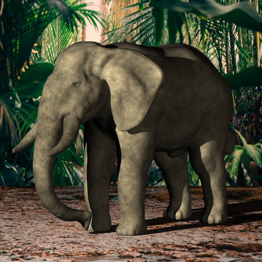
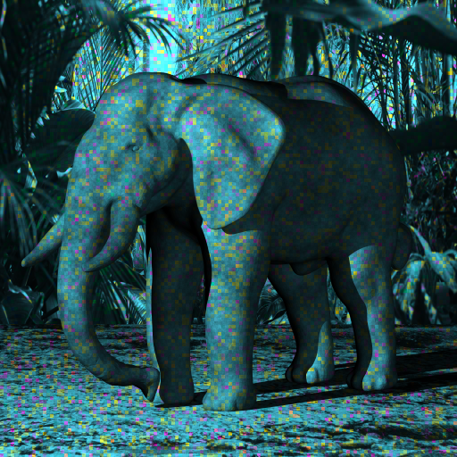
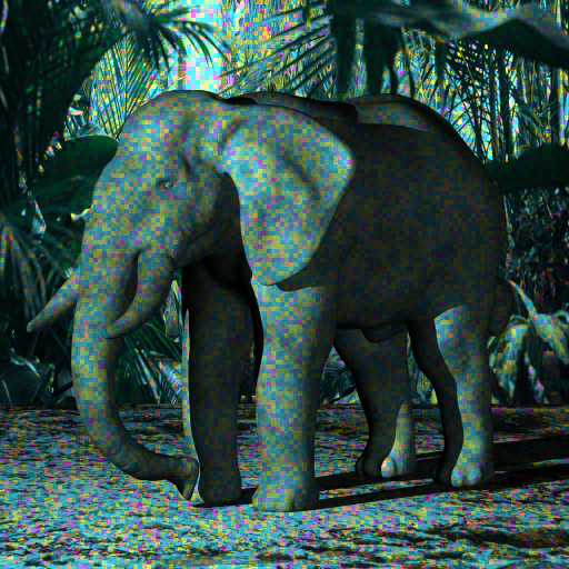
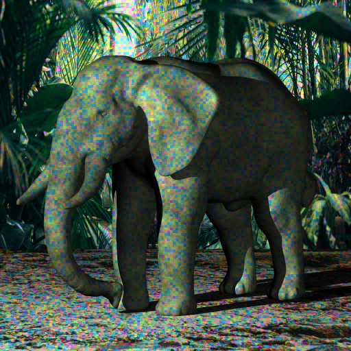
PSNR	18.1089	18.3892	19.4972	21.2688
5D AMDE
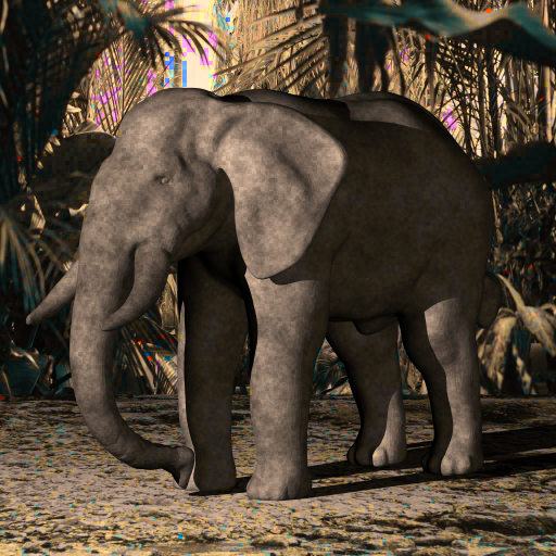
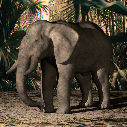
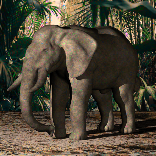
PSNR	24.8808	25.0373	26.4341	28.7968

Figure 3: 5D CS Performance comparison (5D DCT, 5D AMDE) of reconstruction results using different number of snapshots of Elephant scene. Captions are identical to Fig. 4.

Furthermore, Fig. 4 presents a comparative visualization of the reconstruction results of the spectral light field for all scenes in Table 1 using three snapshots. As expected, 5D CS using the AMDE basis achieves visually identical results when compared to 1D AMDE. And 5D AMDE outperforms the 5D CS with the DCT basis as 5D DCT cannot faithfully recover spectral information.

Ground Truth	5D DCT	1D AMDE	5D AMDE
Bust
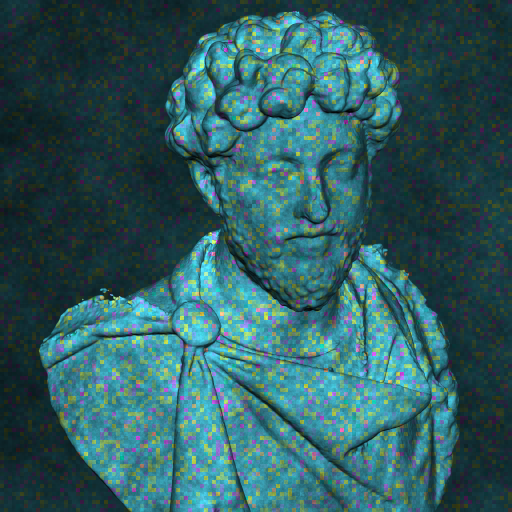
PSNR	25.4520	32.1021	32.1021
Cabin
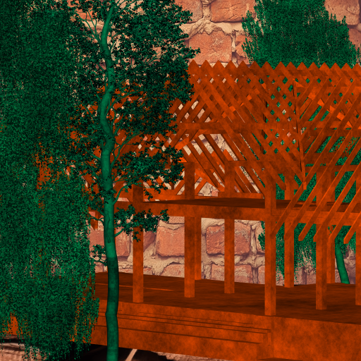
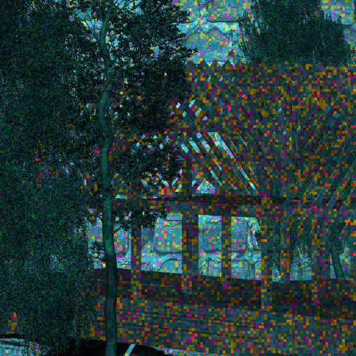
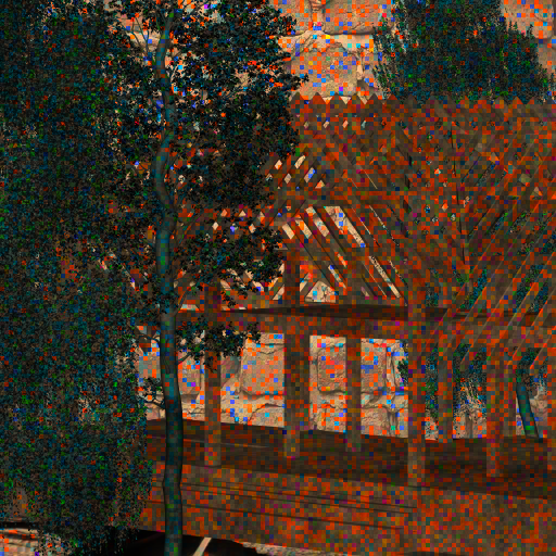
PSNR	16.1041	21.5743	21.5743
Circles
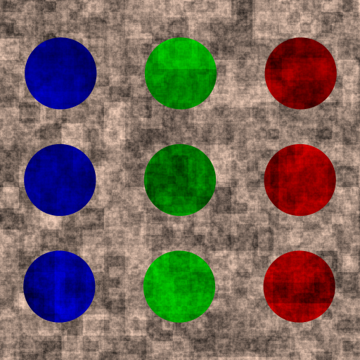
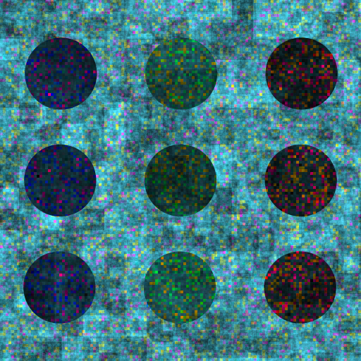
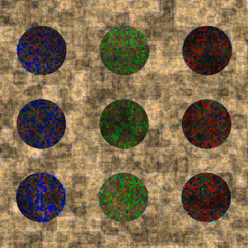
PSNR	15.6698	18.9974	18.9974
Dots
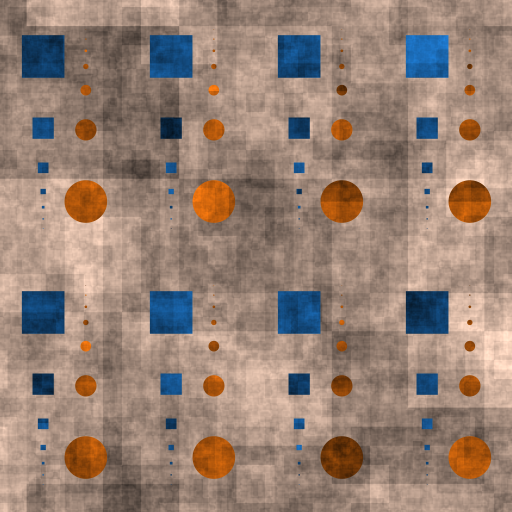
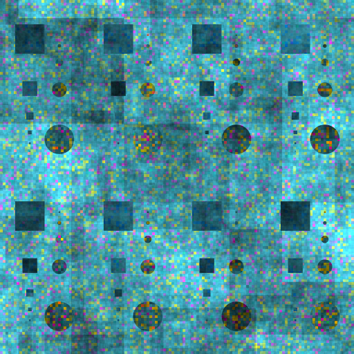
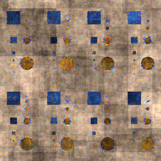
PSNR	16.1914	24.7977	24.7977
Elephant
PSNR	18.3892	25.0373	25.0373

Figure 4: Performance comparison of Reconstruction Results of 5D DCT, 1D AMDE and 5D AMDE of five test spectral light fields using three snapshots. Evaluation metric PSNR in dB. The multi-spectral channels are converted to RGB according to CIE 1913 and CIE D65. The images are chosen as the angular image [2 3] out of the $5\times 5$ reconstructed views.

5 Conclusions

This paper introduced a sensing and reconstruction method for fast multispectral light field acquisition. We believe that our novel $n$D formulation, and in particular the one-hot sampling strategy, opens up new research directions for fast acquisition of other data modalities in computer graphics, e.g. BRDFs, BTF, and light field videos. Multidimensional sensing and dictionary learning allows us to have different sampling strategies for each dimension. For instance, one can choose to take full spectral information and sub-sample the angular information. Hence, our $n$D formulation facilitates the design of new visual data acquisition devices. Another interesting aspect of the proposed method is the utilization of learned dictionaries, which we show to outperform analytical dictionaries such as DCT.

REFERENCES

- Aharon et al., 2006 Aharon, M., Elad, M., and Bruckstein, A. (2006). K-SVD: An algorithm for designing overcomplete dictionaries for sparse representation. IEEE Transactions on Signal Processing, 54(11):4311–4322.
- Arce et al., 2014 Arce, G. R., Brady, D. J., Carin, L., Arguello, H., and Kittle, D. S. (2014). Compressive Coded Aperture Spectral Imaging: An Introduction. IEEE Signal Processing Magazine, 31(1):105–115. Conference Name: IEEE Signal Processing Magazine.
- Babacan et al., 2009 Babacan, S. D., Ansorge, R., Luessi, M., Molina, R., and Katsaggelos, A. K. (2009). Compressive sensing of light fields. In Proceedings of the 16th IEEE ICIP, ICIP’09, page 2313–2316. IEEE Press.
- Candes and Wakin, 2008 Candes, E. J. and Wakin, M. B. (2008). An Introduction To Compressive Sampling. IEEE Signal Processing Magazine, 25(2):21–30. Conference Name: IEEE Signal Processing Magazine.
- Duarte and Baraniuk, 2012 Duarte, M. F. and Baraniuk, R. G. (2012). Kronecker Compressive Sensing. IEEE Transactions on Image Processing, 21(2):494–504. Conference Name: IEEE Transactions on Image Processing.
- Ghaffari et al., 2009 Ghaffari, A., Babaie-Zadeh, M., and Jutten, C. (2009). Sparse decomposition of two dimensional signals. In 2009 IEEE International Conference on Acoustics, Speech and Signal Processing, pages 3157–3160.
- Gortler et al., 1996 Gortler, S. J., Grzeszczuk, R., Szeliski, R., and Cohen, M. F. (1996). The lumigraph. In Proceedings of the 23rd annual conference on Computer graphics and interactive techniques, SIGGRAPH ’96, pages 43–54, New York, NY, USA. ACM.
- Hua et al., 2022 Hua, X., Wang, Y., Wang, S., Zou, X., Zhou, Y., Li, L., Yan, F., Cao, X., Xiao, S., Tsai, D. P., Han, J., Wang, Z., and Zhu, S. (2022). Ultra-compact snapshot spectral light-field imaging. Nature Communications, 13(1):2732. Number: 1 Publisher: Nature Publishing Group.
- Huang et al., 2022 Huang, L., Luo, R., Liu, X., and Hao, X. (2022). Spectral imaging with deep learning. Light: Science & Applications, 11(1):61.
- Kolda and Bader, 2009 Kolda, T. G. and Bader, B. W. (2009). Tensor decompositions and applications. SIAM Review, 51(3):455–500.
- Levoy and Hanrahan, 1996 Levoy, M. and Hanrahan, P. (1996). Light field rendering. In Proceedings of the 23rd annual conference on Computer graphics and interactive techniques - SIGGRAPH ’96, pages 31–42, Not Known. ACM Press.
- Liang et al., 2008 Liang, C.-K., Lin, T.-H., Wong, B.-Y., Liu, C., and Chen, H. H. (2008). Programmable aperture photography: Multiplexed light field acquisition. ACM Trans. Graph., 27(3):1–10.
- Marquez et al., 2020 Marquez, M., Rueda-Chacon, H., and Arguello, H. (2020). Compressive Spectral Light Field Image Reconstruction via Online Tensor Representation. IEEE Transactions on Image Processing, 29:3558–3568.
- Marwah et al., 2013 Marwah, K., Wetzstein, G., Bando, Y., and Raskar, R. (2013). Compressive light field photography using overcomplete dictionaries and optimized projections. ACM Transactions on Graphics, 32(4):1–12.
- Miandji et al., 2019 Miandji, E., Hajisharif, S., and Unger, J. (2019). A Unified Framework for Compression and Compressed Sensing of Light Fields and Light Field Videos. ACM Transactions on Graphics, 38(3):1–18.
- Mohimani et al., 2010 Mohimani, H., Babaie-Zadeh, M., Gorodnitsky, I., and Jutten, C. (2010). Sparse Recovery using Smoothed (SL0): Convergence Analysis. arXiv:1001.5073 [cs, math].
- Ng et al., 2005 Ng, R., Levoy, M., Brédif, M., Duval, G., Horowitz, M., and Hanrahan, P. (2005). Light Field Photography with a Hand-held Plenoptic Camera. Tech Report CSTR 2005-02, Stanford university.
- Schambach and Heizmann, 2020 Schambach, M. and Heizmann, M. (2020). A Multispectral Light Field Dataset and Framework for Light Field Deep Learning. IEEE Access, 8:193492–193502. Conference Name: IEEE Access.
- Schambach et al., 2021 Schambach, M., Shi, J., and Heizmann, M. (2021). Spectral Reconstruction and Disparity from Spatio-Spectrally Coded Light Fields via Multi-Task Deep Learning. arXiv:2103.10179 [cs].
- Wilburn et al., 2005 Wilburn, B., Joshi, N., Vaish, V., Talvala, E.-V., Antunez, E., Barth, A., Adams, A., Horowitz, M., and Levoy, M. (2005). High performance imaging using large camera arrays. ACM Trans. Graph., 24(3):765–776.
- Xiong et al., 2017 Xiong, Z., Wang, L., Li, H., Liu, D., and Wu, F. (2017). Snapshot Hyperspectral Light Field Imaging. In 2017 IEEE Conference on Computer Vision and Pattern Recognition (CVPR), pages 6873–6881, Honolulu, HI. IEEE.
- Yuan et al., 2021 Yuan, X., Brady, D. J., and Katsaggelos, A. K. (2021). Snapshot Compressive Imaging: Theory, Algorithms, and Applications. IEEE Signal Processing Magazine, 38(2):65–88.