Exact Universal Characterization of Chiral-Symmetric Higher-Order Topological Phases

Abstract

Utilizing a series of Bott indices formulated through polynomials of position operators, we establish a comprehensive framework for characterizing topological zero-energy corner states in systems with chiral symmetry. Our framework covers systems with arbitrary shape, including topological phases that are not characterizable by previously proposed invariants such as multipole moments or multipole chiral numbers. A key feature of our framework is its ability to capture the real-space pattern of zero-energy corner states. We provide a rigorous analytical proof of its higher-order correspondence. To demonstrate the effectiveness of our theory, we examine several model systems with representative patterns of zero-energy corner states that previous frameworks fail to classify.

The exploration of higher-order topological phases (HOTPs), encompassing insulators [1, 2, 3, 4, 5, 6, 7, 8, 9, 10, 11, 12], semimetals [13, 14, 15, 16, 17], and superconductors [7, 8, 18, 19, 20, 21, 22, 23, 24], extends beyond the realm of first-order topological phases [25], suggesting a generalized bulk-boundary correspondence [26, 27]. Higher-order multipoles [1, 4, 6], such as quadrupole $q_{xy}$, have been introduced to characterize the corner states in higher-order topological insulators (HOTIs). A notable development is the introduction of the multipole chiral number [28], aimed at capturing the higher-order topology of chiral-symmetric systems. However, limitations and inconsistencies in these advancements have been identified, as detailed in recent studies [29, 30, 31, 32, 33, 34]. Specifically, studies [30, 31, 35] have reported a breakdown in the correspondence between the quadrupole moment (equivalently, the multipole chiral number) and HOTPs in chiral symmetric systems, due to the lack of an exact correspondence relationship. Furthermore, a unified characterization of HOTPs in systems with arbitrary shape has not been provided. Additionally, a variety of patterns of higher-order topological states can emerge. For instance, consider a scenario where a topological Benalcazar-Bernevig-Hughes model [1, 1] is coupled with a chiral-symmetric system possessing zero-energy corner states (ZECSs) located diagonally in a sqaure system [8, 36] while preserving chiral symmetry. The combined system exhibits varying numbers of ZECSs localized at different corners. We refer to this variability in the distribution of corner states as the ‘pattern of corner states’, as illustrated in Fig. 1. However, unlike the well-established first-order topological classification [25], these patterns of ZECSs still lack a comprehensive theoretical framework for their characterization.

In this Letter, we address all the questions mentioned above and provide a framework to characterize all the possible patterns of ZECSs with an exact relationship. Our approach involves a series of Bott indices defined by polynomials of position operators. It provides a universal characterization of chiral-symmetric $n$-th ($n$ is the system dimension) order topological phases for system shapes with $m$ corners ($m>1$ is an arbitrary integer), including the patterns of corner states. Thus, our work establishes an exact correspondence between those Bott indices and ZECSs.

Bott indices and polynomials of position operators.— We consider a Hamiltonian $H$ in an $n$-dimensional lattice with chiral symmetry $\Pi H\Pi^{-1}=-H$, where $\Pi$ is a unitary matrix representing the chiral operator. We take the eigenbasis of $\Pi$ and rewrite the Hamiltonian,

$$H=\left(\begin{matrix}0&h\\ h^{\dagger}&0\\ \end{matrix}\right).$$ (1)

We denote $q=U_{A}U_{B}^{\dagger}$ based on the singular value decomposition of $h$ with size $N$: $h=U_{A}\Sigma U_{B}^{\dagger}$, where $U_{\alpha}=\left[\Psi_{\alpha,1},\dots,\Psi_{\alpha,N}\right],\text{ }\alpha\in\{\text{A,B}\}$, and A (B) labels the eigenspaces of chiral operator $\Pi$ with eigenvalue $+1$ ($-1$). $\Sigma$ is a diagonal matrix with nonnegative elements. The eigenstates of $H$ can be written as $|\Psi_{i}\rangle=(1/\sqrt{2})[\Psi_{A,i},\Psi_{B,i}]^{T}$. Our focus is on insulating states, meaning that the appearance of topological ZECSs requires the existence of energy gaps for all states except those that are localized at corners.

For $n=1$, the problem returns to characterizing the first-order topological phase in AIII class, which has been extensively studied utilizing the winding number [25] and the Bott index [37]. We focus on the Bott index [38, 39].

$$\nu_{(\text{1D})} =\operatorname{Bott}\left(e^{2\pi i\frac{X}{L}},q\right),$$ (2)

$$\operatorname{Bott}\left(e^{2\pi i\frac{X}{L}},q\right) :=\frac{1}{2\pi i}\operatorname{Tr}\operatorname{Log}\left(e^{2\pi i\frac{X}{L}}qe^{-2\pi i\frac{X}{L}}q^{\dagger}\right),$$

where $X$ is the $x$-direction position operator, $L$ is the system length, $\operatorname{Log}$ is the principal logarithm, and $q$ is derived under periodic boundary conditions. Considering $q$ as a representation of the states and ${X}/{L}$ as a polynomial that functions as a topology-measuring ruler, a critical question arises: Is it possible to formulate a measurement polynomial in the Bott index to capture the $n$-th order topological phases for an arbitrary $n$-dimensional Hamiltonian with chiral symmetry?

Here, we aim to answer this question by proposing a general scheme to construct Bott indices that involves the polynomial $f$ of position operators and the polynomial $g$ of system length $L$,

$$\hat{M} =e^{2\pi i\frac{f(X,Y,Z,\dots)}{g(L)}},$$ (3)

$$\nu =\operatorname{Bott}\left(\hat{M},q\right).$$

For simplicity, we assume that the system shape is regular.

In addition, to fully describe the $n$-th order topological phases in chiral-symmetric systems, we define the following configuration vector of corner states for system shapes with $m$ corners.

$$\boldsymbol{\chi}_{m}=\left(N_{1}^{(B)}-N_{1}^{(A)},\dots,N_{m}^{(B)}-N_{m}^{(A)}\right)^{\mathrm{T}},$$ (4)

where $N_{i}^{(A)}$ and $N_{i}^{(B)}$ denote the number of corner states localized in the $i$-th corner and with $+$ and $-$ chirality, respectively. Given the zero trace of the chiral operator, it follows that $\sum_{i=1}^{m}{\chi}_{m}^{(i)}=0$, where ${\chi}_{m}^{(i)}$ denotes the $i$-th component of $\boldsymbol{\chi}_{m}$. The goal of our scheme is to find a correspondence between the ZECSs patten $\boldsymbol{\chi}_{m}$ and the Bott index $\nu$.

It should be emphasized that we now turn to consider Hamiltonians with open boundary conditions, in contrast to the periodic boundary conditions typically assumed. This approach renders $f(X,Y,Z,\dots)/g(L)$ well-defined, circumventing the difficulties inherent in operator-based formulations within periodic systems [40] and making it possible to prove an exact correspondence between $\boldsymbol{\chi}_{m}$ and $\nu$. Also, we emphasize that the Bott index that we define captures the topology of bulk and edge states, rather than directly counts corner states, which is demonstrated in Eq. (12). However, adopting open boundary conditions introduces certain challenges: the operator $q$ is not unique when zero-energy states are present. Nevertheless, $\nu$ will remain unchanged, provided that $f$ and $g$ are properly constructed (see details in Eq. (13)).

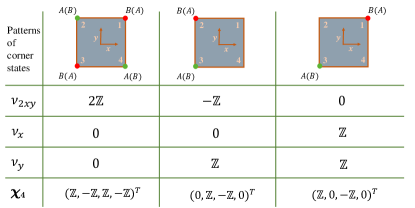
Figure 1: Three patterns of corner states with linearly independent configuration vectors in systems with square shape, along with three Bott indices that satisfy $\det\mathcal{M}\neq 0$. As described by Eq. (18) and Eq. (19), all possible ZECS patterns can be characterized by these three Bott indices.

Bott index-ZECSs correspondence.— We begin by introducing the following theorem.

Theorem 1.

If no zero-energy corner states exist in a system with chiral symmetry, finite coupling range, and energy gap, then the following conclusion holds true in the limit of large system size $L\to\infty$.

$$-1\notin\sigma(\hat{M}q\hat{M}^{\dagger}q^{\dagger}),$$ (5)

$$\operatorname{Bott}\left(\hat{M},q\right)=0,$$

where $f$ and $g$ in $\hat{M}$ can be arbitrary polynomials with $\operatorname{deg}(f)=\operatorname{deg}(g)$, and $\sigma$ denotes the set of eigenvalues of a matrix.

The proof of this theorem is available in Supplemental Material (SM) [41]. Based on Theorem 1, we conclude that if the Bott index $\nu\neq 0$, then ZECSs exist. Furthermore, we establish an analytical exact correspondence between the value of a Bott index $\nu$ and the configuration vector of ZECSs $\boldsymbol{\chi}_{m}$ in systems with $m$ corners.

$$\nu=\sum_{i=1}^{m}\operatorname{sign}\left(f(\boldsymbol{x}_{i})/g(L)\right)\chi_{m}^{(i)}/2\in\mathbb{Z},$$ (6)

where $\boldsymbol{x}_{i}$ denotes the position vector of the $i$-th corner, and polynomials $f$ and $g$ follow the rule below.

1. $f(\boldsymbol{x}_{c})=\pm g(L)/2$, where $\boldsymbol{x}_{c}$ represents the position vector of corners in which ZECSs may appear.

Equation (6) is proved as follows. First, we rewrite $\nu$ as

$$\nu =\frac{1}{2\pi i}\operatorname{Tr}\operatorname{Log}\left(U_{A}^{\dagger}\hat{M}U_{A}U_{B}^{\dagger}\hat{M}^{\dagger}U_{B}\right)$$ (7)

$$=\frac{1}{2\pi}\sum_{j}\lambda_{j},$$

where $e^{i\lambda_{j}}$ with $\lambda_{j}\in(-\pi,\pi)$, is the eigenvalue of $U_{A}^{\dagger}\hat{M}U_{A}U_{B}^{\dagger}\hat{M}^{\dagger}U_{B}$ [39]. We now consider $U_{\alpha}^{\dagger}\hat{M}U_{\alpha}$, where $\alpha\in\{A,B\}$. In the position basis, $U_{\alpha}$ can be written as:

$$U_{\alpha}=\left[\Psi_{\alpha,\text{bulk}}\quad\Psi_{\alpha,\text{edge}}\quad\Psi_{\alpha,\text{corner}}\right],$$ (8)

where $\Psi_{\alpha,\text{bulk (edge,corner)}}$ denotes the $\alpha$ component of wavefunctions extended in the bulk (edge, corner) of the system. Consequently, we obtain the following result.

$$\langle\Psi_{\alpha,\beta_{1}}\mid\hat{M}\mid\Psi_{\alpha,\beta_{2}}\rangle\stackrel{{\scriptstyle L\to\infty}}{{\longrightarrow}}0,\quad\beta_{1}\neq\beta_{2},$$ (9)

for $\beta_{1},\beta_{2}\in\{\text{bulk},\text{edge},\text{corner}\}$. Therefore, $U_{\alpha}^{\dagger}\hat{M}U_{\alpha}$ becomes a block diagonal matrix as $L\rightarrow\infty$,

$$U_{\alpha}^{\dagger}\hat{M}U_{\alpha}=\bigoplus_{\beta\in\{\text{bulk},\text{edge},\text{corner}\}}U_{\alpha,\beta}^{\dagger}\hat{M}U_{\alpha,\beta},$$ (10)

where $U_{\alpha,\beta}$ are matrices composed of the $\alpha$ component of eigenstates $\Psi_{\beta}$ reside in $\beta$. Similarly, $U_{A}^{\dagger}\hat{M}U_{A}U_{B}^{\dagger}\hat{M}^{\dagger}U_{B}$ also becomes a block diagonal matrix.

In the limit $L\to\infty$, corner states $\Psi_{\alpha,\text{corner}}$ will become the eigenstates of the position operator $\boldsymbol{X}$ with eigenvalue $\boldsymbol{x}_{\alpha,c}$, the position vector of the corner where it is localized. Therefore, $\hat{M}\Psi_{\alpha,\text{corner}}=e^{2\pi if(\boldsymbol{x}_{\alpha,c})/g(L)}\Psi_{\alpha,\text{corner}}=-\Psi_{\alpha,\text{corner}}$, according to the Rule 1 in our strategy. Furthermore, it follows that

$$U_{\alpha,\text{corner}}^{\dagger}\hat{M}U_{\alpha,\text{corner}}=-U_{\alpha,\text{corner}}^{\dagger}U_{\alpha,\text{corner}} =-\mathbbm{1}$$ (11)

$$U_{A,\text{corner}}^{\dagger}\hat{M}U_{A,\text{corner}}U_{B,\text{corner}}^{\dagger}\hat{M}^{\dagger}U_{B,\text{corner}} =\mathbbm{1}.$$

From this result, we find that the contribution of corner states to the Bott index equals zero, since

$$\operatorname{Bott}\left(\hat{M},q\right)=\frac{1}{2\pi i}\sum_{\beta}\operatorname{Tr}\operatorname{Log}\left(U_{A,\beta}^{\dagger}\hat{M}U_{A,\beta}U_{B,\beta}^{\dagger}\hat{M}^{\dagger}U_{B,\beta}\right),$$ (12)

and $\operatorname{Tr}\operatorname{Log}\left(\mathbbm{1}\right)=0$. Thus, a non-zero Bott index comes from the topology of edge states and bulk states.

Now we are able to demonstrate that the non-uniqueness of the operator $q$ does not alter the previously defined Bott index. When eigenstates with zero energy appear, the operator $q$ is not unique due to arbitrary unitary transformations, represented by $W_{A}$ on $U_{A,\text{corner}}$ and $W_{B}$ on $U_{B,\text{corner}}$. It follows that

$$W_{\alpha}^{\dagger}U_{\alpha,\text{corner}}^{\dagger}\hat{M}U_{\alpha,\text{corner}}W_{\alpha} =-W_{\alpha}^{\dagger}U_{\alpha,\text{corner}}^{\dagger}U_{\alpha,\text{corner}}W_{\alpha}$$ (13)

$$=-\mathbbm{1}.$$

This agrees with the result in Eq. (11), regardless of arbitrary transformation.

Second, we define two functions of $s$ for $s\in[0,1]$ with $\hat{M}(s)=\operatorname{exp}[2\pi i\frac{f(X,Y,Z,\dots)\times s}{g(L)}]$ and $\nu(s)=\operatorname{Bott}\left(\hat{M}(s),q\right)$. Thus, we have $\nu(1)=\nu$ and $\nu(s)=1/2\pi\sum_{j}\lambda_{j}(s)$. For a specific pattern of ZECSs $\boldsymbol{\chi}_{m}$, we have

$$\det\left(U_{A,\text{corner}}^{\dagger}\hat{M}(s)U_{A,\text{corner}}U_{B,\text{corner}}^{\dagger}\hat{M}(s)^{\dagger}U_{B,\text{corner}}\right)$$ (14)

$$=e^{i\sum_{j\in\text{corner}}\lambda_{j}(s)}$$

$$=e^{-is\pi\sum_{i}^{m}\operatorname{sign}\left(f(\boldsymbol{x}_{i})/g(L)\right)\chi_{m}^{(i)}}.$$

In these equations, the ‘corner’ refers to the set of indices $j$ labeling eigenvalues of the corner block.

Given that $\det(\hat{M}(s)q(\hat{M}(s))^{\dagger}q^{\dagger})=e^{i\sum_{j}\lambda_{j}(s)}=1$, we have

$$e^{i\sum_{j\notin\text{corner}}\lambda_{j}(s)}=e^{-i\sum_{j\in\text{corner}}\lambda_{j}(s)}.$$ (15)

We expect that in the limit $L\to\infty$, $\lambda_{j\notin\text{corner}}(s)$ does not encounter the branch cut of logarithm for $s\in[0,1]$. This conclusion can be reached by applying Theorem 1 to the effective Hamiltonian $\tilde{H}$, which is composed of edge and bulk states and features both a spectral gap and a finite coupling range. The finite coupling range of $\tilde{H}$ is inherited from the finite coupling of $H$, as evidenced by the representation $H=\sum_{j\notin\text{corner}}E_{j}|\Psi_{j}\rangle\langle\Psi_{j}|$ and $\tilde{H}=R\cdot H\cdot R^{T}$, where $R$ is a rectangular matrix that projects onto the Hilbert space of $\tilde{H}$. It follows that

$$\partial_{s}\sum_{j\notin\text{corner}}\lambda_{j}(s)=\pi\sum_{i}^{m}\operatorname{sign}\left(f(\boldsymbol{x}_{i})/g(L)\right)\chi_{m}^{(i)}$$ (16)

Since $\lambda_{j}(0)=0$, we have $\sum_{j\notin\text{corner}}\lambda_{j}(s)=s\pi\sum_{i}^{m}\operatorname{sign}\left(f(\boldsymbol{x}_{i})/g(L)\right)\chi_{m}^{(i)}$. When $s=1$, we obtain

$$\nu=\nu(1) =\frac{1}{2\pi}\sum_{j}\lambda_{j}(1)=\frac{1}{2\pi}\sum_{j\notin\text{corner}}\lambda_{j}(1)$$ (17)

$$=\sum_{i}^{m}\operatorname{sign}\left(f(\boldsymbol{x}_{i})/g(L)\right)\chi_{m}^{(i)}/2,$$

where in the first row we use the result obtained in Eq. (11), which states that $\lambda_{j}(1)=0$ for all $j\in\text{corner}$.

Full characterization of systems with arbitrary shape.— Having established the analytical relationship, we can now characterize all possible ZECS patterns in systems of arbitrary shape, without any prior information on these patterns. This characterization for systems with $m$ corners is achieved by considering the Bott index $\nu^{(i)}_{m}$, derived from implementing $m-1$ distinct polynomials $f_{m}^{(i)}$ that comply with Rule 1, where $i$ is the label of polynomials. By constructing an $m\times m$ matrix $\mathcal{M}$, with $\mathcal{M}_{ij}=\operatorname{sign}\left(f_{m}^{(i)}(\boldsymbol{x}_{j})/g_{m}^{(i)}(L)\right)/2$ for $1\leq i\leq m-1$ and $\mathcal{M}_{mj}=1/2$ (where $j$ labels the corners), we establish a relation between the Bott index $\nu_{m}^{(i)}$ and the configuration vector $\boldsymbol{\chi}_{m}$ defined by Eq. (4) according to Eq. (6).

$$\boldsymbol{\chi}_{m}=\mathcal{M}^{-1}\cdot\left(\nu^{(1)}_{m},\dots,\nu^{(m-1)}_{m},0\right)^{\mathrm{T}},$$ (18)

where we choose a series of polynomials such that $\det\mathcal{M}\neq 0$. By implementing this equation, we characterize all ZECS patterns for systems with $m$ corners.

Taking systems with the square shape as an example, we define three Bott indices $\nu_{2xy}$, $\nu_{x}$, and $\nu_{y}$ corresponding to $f/g$ equaling $2XY/L^{2}$, $X/L$, and $Y/L$ respectively, where $L$ is the side length of the square. As illustrated in Fig. 1, we characterize patterns using Eq. (18), where

$$\mathcal{M}=\frac{1}{2}\begin{pmatrix}1&-1&1&-1\\ 1&-1&-1&1\\ 1&1&-1&-1\\ 1&1&1&1\end{pmatrix}.$$ (19)

For systems shaped as regular hexagons, we define Bott indices $(\nu_{6}^{(1)},\nu_{6}^{(2)},\nu_{6}^{(3)},\nu_{6}^{(4)},\nu_{6}^{(5)})$ with the corresponding $f/g$,

$$\{ (X^{3}-\frac{XY^{2}}{3}+\frac{8Y^{3}}{3\sqrt{3}})/2L^{3},(X^{2}-\frac{4XY}{\sqrt{3}}-\frac{Y^{2}}{3})/2L^{2},$$ (20)

$$(X^{2}+\frac{4XY}{\sqrt{3}}-\frac{Y^{2}}{3})/2L^{2},(X^{3}-3XY^{2})/2L^{3},$$

$$(X^{3}+\frac{7XY^{2}}{3})/2L^{3}\},$$

where $L$ is again the side length of the hexagon. As a supplement, we provide a series of polynomials and associated matrices $\mathcal{M}$ for systems shaped as $l$-sided regular polygon ($l\in\{4,5,6,8,12\}$) in SM [41], where systems with non-regular shapes are also discussed.

Lattice Models.— We now provide three concrete examples to demonstrate the application of our framework. We note that all calculations of Bott indices are performed in real space.

First, we examine a modified model, informed by two recent papers [30, 31], which incorporates additional diagonal long-range hoppings. These hoppings break separability while maintaining momentum-glide reflection symmetries and chiral symmetry, as depicted in the left panel of Fig. 2(a). The corresponding Bloch Hamiltonian at momentum $\boldsymbol{k}$ can be written in the form of Eq. (1) with

$$h(\boldsymbol{k})= \left(\begin{matrix}t_{x}+t_{x}^{\prime}e^{-ik_{x}}&t_{y}+t_{y}^{\prime}e^{-ik_{y}}\\ t_{y}-t_{y}^{\prime}e^{ik_{y}}&-t_{x}+t_{x}^{\prime}e^{ik_{x}}\\ \end{matrix}\right)$$ (21)

$$+w_{d}\left(\begin{matrix}ie^{-ik_{x}}\cos k_{y}&ie^{-ik_{y}}\cos k_{x}\\ ie^{ik_{y}}\cos k_{x}&-ie^{ik_{x}}\cos k_{y}\\ \end{matrix}\right),$$

where $t_{x(y)}$, $t_{x(y)}^{\prime}$, and $w_{d}$ are the nearest hoppings within unit cells, between unit cells, and along the diagonal directions, respectively. We set $t_{x}^{\prime}=t_{y}^{\prime}=1$. This system hosts one ZECS at each corner, which cannot be accurately characterized by the quadrupole moment $q_{xy}$ [4, 42, 43, 44] or the multipole chiral number $N_{xy}$ proposed in Ref. [28] (definitions provided in SM [41]), mirroring findings reported in the aforementioned two papers [30, 31]. However, the Bott index $\nu_{2xy}$ is in precise agreement with the existence of ZECSs, unlike $q_{xy}$ and $N_{xy}$, as depicted by the density of states as a function of $t_{x}$ in Fig. 2(a). In addition, calculation shows that Bott indices $\nu_{x}$ and $\nu_{y}$ always equal zero, consistent with the pattern of the ZECSs (see Fig. 1).

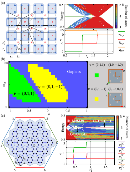
Figure 2: (a) Left panel: Schematic of the model in Eq. (21). For clarity, we do not show all non-nearest-neighbor hoppings. The dashed lines represent an additional phase factor of $-1$ such that the system possesses the staggered $\pi$ flux. Right panel: Density of states for this system and corresponding $\nu_{2xy}$, $q_{xy}$ and $N_{xy}$ as functions of $t_{x}$ with $t_{y}=0.1$, $t_{x}^{\prime}=t_{y}^{\prime}$, $w_{d}=0.8$. The system length $L=50$. (b) Phase diagram of $\boldsymbol{\nu}$ in the system described by Eq.(22) as a function of $\delta$ and $m_{2}$ with $m_{1}=1$. The right panel shows the patterns of ZECSs corresponding to $\boldsymbol{\nu}$. (c) Left panel: Schematic of the model in Eq. (23). Right panel: The upper part shows the density of states for this system and the configuration vectors $\boldsymbol{\chi}_{6}$ for three higher-order topological phases. The lower part displays the corresponding Bott indices $\nu^{(1,\dots,5)}_{6}$ as functions of $t_{2}^{\prime}$. We fix $t_{1}=1/10$, $t_{2}=1/3$, $t_{3}=1/4$, $t_{4}=3/10$, $t_{5}=1/4$, $t_{6}=1/2$, $t_{1}^{\prime}=t_{3}^{\prime}=1$ and the system length $L=30$.

Second, we study another system with ZECSs located only at two diagonal corners of a square. The corresponding model has mirror-symmetry-protected corner states, as reported by Refs. [8, 36], and we add a mirror-symmetry-breaking $\delta$ term to it.

$$h(\boldsymbol{k})= (\delta+m_{2}-i\sin k_{y})\mathbbm{1}+(-\sin k_{x}+im_{2})\tau_{z}$$ (22)

$$+(-m_{1}-\cos k_{x}-\cos k_{y})\tau_{x},$$

where $\tau_{i}$ represents the Pauli matrix. When $\delta=0$, this system possesses diagonal and anti-diagonal mirror symmetries. The HOTPs in this system, which appear even without mirror symmetries ($\delta\neq 0$), can be comprehensively characterized by the three Bott indices $\boldsymbol{\nu}=(\nu_{2xy},\nu_{x},\nu_{y})$. The phase diagram of $\boldsymbol{\nu}$ as a function of $\delta$ and $m_{2}$ is shown in Fig. 2(b), illustrating that two HOTPs, where two ZECSs are located at diagonal or anti-diagonal corners, are separated by gapless edge phases. The relationship between the Bott indices $\boldsymbol{\nu}$ of each phase and the ZECSs configuration vector $\boldsymbol{\chi}_{4}$ is described by Eq. (18) with $\mathcal{M}$ in Eq. (19), as illustrated in the right panel of Fig. 2(b).

Finally, we study a lattice model with a regular hexagon shape, as shown in the left panel of Fig. 2(c):

$$h(\boldsymbol{k})=\begin{pmatrix}t_{1}&t_{2}&t_{3}^{\prime}e^{\frac{i(k_{x}-\sqrt{3}k_{y})}{2}}\\ t_{1}^{\prime}e^{-ik_{x}}&t_{3}&t_{4}\\ t_{5}&t_{2}^{\prime}e^{\frac{i(k_{x}+\sqrt{3}k_{y})}{2}}&t_{6}\end{pmatrix}.$$ (23)

When $t_{i}=t$ and $t_{j}^{\prime}=t^{\prime}$ for $i\in\{1,\dots,6\},j\in\{1,2,3\}$, the system possesses $C_{6}$ symmetry with its ZECSs characterized by the $C_{6}$ topological indices [9]. However, in the absence of $C_{6}$ and $C_{2}$ symmetries, the ZECSs still emerge, and HOTPs in this system exhibit a varying number of ZECSs. This is illustrated by the density of states as a function of $t_{2}^{\prime}$, as shown in the right panel of Fig. 2(c). As $t_{2}^{\prime}$ increases from $0.3$ to $1.8$ (with other parameters specified in Fig. 2), the system changes from a HOTP with two ZECSs to a HOTP with four ZECSs, and finally to a HOTP with six ZECSs, where the edge gap closes at each transition. In Fig. 2(c), we also show the Bott indices $(\nu_{6}^{(1)},\nu_{6}^{(2)},\nu_{6}^{(3)},\nu_{6}^{(4)},\nu_{6}^{(5)})$ as functions of $t_{2}^{\prime}$, which fully characterizes each phase according to Eq. (18).

Conclusion.— In summary, we have established a comprehensive framework to universally characterize $n$-th order topological phases in $n$-dimensional systems (see SM [41] for demonstration using more lattice models). Firstly, we establish an exact correspondence between the Bott index and the HOTPs, successfully addressing the anomalies reported in earlier studies [30, 31]. Secondly, by providing a general strategy to construct the Bott index, our framework applies to $n$-dimensional systems of arbitrary shape. Furthermore, our framework enables the characterization of all possible patterns of topological ZECSs using a series of Bott indices. We expect a wide variety of applications of our theory to characterize HOTPs, including, for example, topological superconductors with Majorana corner modes.

Acknowledgements.— J.-Z. L. and M.X. are supported by the National Key Research and Development Program of China (Grant No. 2022YFA1404900), the National Natural Science Foundation of China (Grant No. 12334015, Grant No. 12274332 and Grant No. 12321161645). X.-J. L. and F.W. are supported by Key Research and Development Program of Hubei Province (Grant No. 2022BAA017).

Supplemental Material for
“Exact Universal Characterization of Chiral-Symmetric Higher-order Topological phases”

I Mathematical Structure of Bott Index

I.1 Notations

$\sigma(\cdot)$ denotes the set of eigenvalues of a matrix.

$\underset{S}{\text{sup}}P$ represents the supremum of the values taken by $P$ over a set $S$.

$\parallel\cdot\parallel$ denotes the spectral norm of a matrix (the largest singular value of a matrix). This norm is induced by the Euclidean norm, $|\cdot|$, for vectors and is given by $\parallel A\parallel=\underset{x\neq 0}{\text{sup}}\frac{|Ax|}{|x|}$, where $x$ is a vector.

For the spectral norm, we have following two inequalities for two square matrices $A$ and $B$,

$$\parallel A+B\parallel \leq\parallel A\parallel+\parallel B\parallel$$ (S1)

$$\parallel AB\parallel \leq\parallel A\parallel\parallel B\parallel.$$ (S2)

$\operatorname{dist}(n,m)$ represents the Euclidean distance function in position space.

$\mathcal{O}$ denotes the order of approximation.

I.2 Bott Index

Definition I.1.

Given two unitary matrices $U$ and $V$, such that ${-1}\notin\sigma(UVU^{\dagger}V^{\dagger})$ or equivalently such that $\parallel[U,V]\parallel<2$, their Bott index is defined as:

$$\operatorname{Bott}(U,V):=\frac{1}{2\pi i}\operatorname{Tr}\operatorname{Log}\left(UVU^{\dagger}V^{\dagger}\right).$$ (S3)

Remark 1.

From

$$\parallel UVU^{\dagger}V^{\dagger}-\mathbbm{1}\parallel=\parallel(UV-VU)U^{\dagger}V^{\dagger}\parallel=\parallel[U,V]\parallel,$$ (S4)

we deduce that ${-1}\in\sigma(UVU^{\dagger}V^{\dagger})$ if and only if $\parallel[U,V]\parallel=2$. Given the unitarity of $U$ and $V$, we have $\parallel[U,V]\parallel=\parallel(UV-VU)\parallel\leq\parallel UV\parallel+\parallel VU\parallel=2$. Thus, since ${-1}\notin\sigma(UVU^{\dagger}V^{\dagger})$ is equivalent to $\parallel[U,V]\parallel\neq 2$, we deduce that ${-1}\notin\sigma(UVU^{\dagger}V^{\dagger})$ is also equivalent to $\parallel[U,V]\parallel<2$.

The Bott index in Definition I.1 is an Integer. This can be obtained by the following [45, 46, 39]. From $\det(UVU^{\dagger}V^{\dagger})=1$, we have $1=\prod_{j}e^{i\theta_{j}}=e^{i\sum_{j}\theta_{j}}$, where $e^{i\theta_{j}}$ with $\theta_{j}\in(-\pi,\pi)$, is the eigenvalue of $UVU^{\dagger}V^{\dagger}$. It follows that $\operatorname{Bott}(U,V)=\frac{1}{2\pi i}\sum_{j}\operatorname{Log}(e^{i\theta_{j}})=\frac{1}{2\pi}\sum_{j}\theta_{j}\in\mathbb{Z}$.

Theorem I.1.

Given two continuous maps $V(s)$ : $[0,1]\to\mathcal{U}(N)$ and $W(s)$ : $[0,1]\to\mathcal{U}(N)$, where $\mathcal{U}(N)$ represents the unitary group, with $V(0)=V$, $W(0)=W$, such that $\parallel[V(s),W(s)]\parallel<2,\forall s\in[0,1]$, then

$$\operatorname{Bott}\left(V(s),W(s)\right)=\operatorname{Bott}(V,W).$$ (S5)

Proof.

The proof of this theorem can be found in Refs. [45, 46]. ∎

As demonstrated by this theorem, Bott index is a topological invariant. A continuous transformation that keeps it well-defined cannot alter the Bott index. With this theorem, we have the following corollary.

Corollary I.1.1.

Consider two unitary matrices $V=e^{iA}$ and $W=e^{iB}$, where $A$ and $B$ are Hermitian matrices. If $\operatorname{Bott}(V,W)\neq 0$, then there exists $s_{0}\in[0,1]$ such that $\parallel[e^{iAs_{0}},e^{iB}]\parallel=2$.

Proof.

Consider the case where $\parallel[e^{iAs_{0}},e^{iB}]\parallel<2$ for all $s_{0}\in[0,1]$. Consequently, according to Theorem I.1, $\operatorname{Bott}\left(e^{iA},e^{iB}\right)=\operatorname{Bott}\left(e^{iA0},e^{iB}\right)=0$. However, since $\operatorname{Bott}\left(e^{iA},e^{iB}\right)\neq 0$, this indicates the existence of at least one value $s_{0}\in[0,1]$ for which $\parallel[e^{iAs_{0}},e^{iB}]\parallel=2$. ∎

Consider an $n$-dimensional Hamiltonian $H$ within a lattice of length $L$ and coupling range $R\ll L$, under open boundary conditions. This implies $H_{n,m}=0$ when $\operatorname{dist}(n,m)>R$ in the position basis. We construct position operators $X,Y,Z,\dots$ according to the dimension of this Hamiltonian. We have the following theorem for $H$ under open boundary conditions.

Theorem I.2.

Consider two polynomials $f(X,Y,Z,\dots)$ and $g(L)$ with $\operatorname{deg}(f)=\operatorname{deg}(g)$. Then,

$$\parallel[e^{2\pi i\frac{f(X,Y,Z,\dots)}{g(L)}},H]\parallel\leq\mathcal{O}\left(\frac{R}{L}\parallel H\parallel\right),$$ (S6)

for $H$ under open boundary conditions.

Proof.

The proof of this theorem follows the ideas of Ref. [46]. We use the Holmgren bound [47, 46] for the norm of a bounded operator $A$.

$$\parallel A\parallel\leq\max\left(\sup_{m\in\mathbb{Z}^{n}}\sum_{n\in\mathbb{Z}^{n}}|\langle m|A|n\rangle|,m\leftrightarrow n\right),$$ (S7)

where $|n\rangle$ and $|m\rangle$ are eigenkets of position operator, and $m\leftrightarrow n$ denotes the exchange of the index $m$ and $n$ in the supremum and in the sum. A proof of this bound can be found in Ref. [47] and Ref. [46]. Thus, we have

$$\parallel[e^{2\pi i\frac{f(X,Y,Z,\dots)}{g(L)}},H]\parallel$$ (S8)

$$\leq\max\left(\sup_{m\in\mathbb{Z}^{n}}\sum_{n\in\mathbb{Z}^{n}}|\langle m|[e^{2\pi i\frac{f(X,Y,Z,\dots)}{g(L)}},H]|n\rangle|,m\leftrightarrow n\right).$$

Notice that

$$\langle m|[e^{2\pi i\frac{f(X,Y,Z,\dots)}{g(L)}},H]|n\rangle=(e^{2\pi i\frac{f(\boldsymbol{x}_{m})}{g(L)}}-e^{2\pi i\frac{f(\boldsymbol{x}_{n})}{g(L)}})\langle m|H|n\rangle,$$ (S9)

where $\boldsymbol{x}_{m}$ and $\boldsymbol{x}_{n}$ are the coordinate of $|m\rangle$ and $|n\rangle$, respectively. Therefore,

$$\|\bigl{[}e^{2\pi i\frac{f(X,Y,Z,\dots)}{g(L)}},H\bigr{]}\|$$

$$\leq\max_{m\leftrightarrow n}\Biggl{(}\sup_{m\in\mathbb{Z}^{n}}\sum_{\begin{subarray}{c}\text{dist}(n,m)\leq R\end{subarray}}\bigl{|}e^{2\pi i\frac{f(\boldsymbol{x}_{m})}{g(L)}}-e^{2\pi i\frac{f(\boldsymbol{x}_{n})}{g(L)}}\bigr{|}|\langle m|H|n\rangle|\Biggr{)}.$$

Observe that for $\text{dist}(n,m)\leq R$, the following relationship holds:

$$|e^{2\pi i\frac{f(\boldsymbol{x}_{m})}{g(L)}}-e^{2\pi i\frac{f(\boldsymbol{x}_{n})}{g(L)}}| =|e^{2\pi i\frac{f(\boldsymbol{x}_{m})}{g(L)}}(1-e^{2\pi i\frac{f(\boldsymbol{x}_{n})-f(\boldsymbol{x}_{m})}{g(L)}})|$$ (S10)

$$\leq\mathcal{O}(\frac{R}{L}),$$

where we use $\frac{f(\boldsymbol{x}_{n})-f(\boldsymbol{x}_{m})}{g(L)}\leq\mathcal{O}\left(\frac{R}{L}\right)$. This is obtained by considering the Taylor expansion of $f$ at $\boldsymbol{x}_{m}$

$$\frac{f(\boldsymbol{x}_{n})}{g(L)} =\frac{f(\boldsymbol{x}_{m})+\nabla f(\boldsymbol{x})|_{\boldsymbol{x}=\boldsymbol{x}_{m}}\cdot(\boldsymbol{x}_{n}-\boldsymbol{x}_{m})+\cdots}{g(L)}$$ (S11)

$$\leq\frac{f(\boldsymbol{x}_{m})}{g(L)}+\mathcal{O}(R/L)+\mathcal{O}(R/L^{2})+\cdots,$$

where we use $\operatorname{deg}(f)=\operatorname{deg}(g)$. It follows that

$$\parallel[e^{2\pi i\frac{f(X,Y,Z,\dots)}{g(L)}},H]\parallel\leq\mathcal{O}\left(\frac{R}{L}\parallel H\parallel\right).$$

∎

Lemma 2.

Given a Hamiltonian $H$, as defined above, with a spectral gap $\Delta E$, the spectral projector $P$ is called the Fermi projection, defined as follows:

$$P=\sum_{i=1}^{N_{occ}}|\Psi_{i}\rangle\langle\Psi_{i}|.$$ (S12)

The summation is taken over all occupied states. The following relationship holds true,

$$\parallel[e^{2\pi i\frac{f(X,Y,Z,\dots)}{g(L)}},P]\parallel\leq\mathcal{O}\left(\frac{R}{L}\frac{\parallel H\parallel}{\Delta E}\right),$$ (S13)

for arbitrary polynomials $f$ and $g$ with $\operatorname{deg}(f)=\operatorname{deg}(g)$.

Proof.

The proof of this Lemma still follows the ideas of Ref. [46]. For $z\notin\sigma(H)$ and any matrix $A$ with the size of $H$, we have an equality

$$\left[A,(H-z)^{-1}\right] =(H-z)^{-1}\left[(H-z),A\right](H-z)^{-1}$$ (S14)

$$=(H-z)^{-1}\left[H,A\right](H-z)^{-1}.$$

Now, we use the contour integral representation of the Fermi projection $P$, with the loop $\Gamma$ in the complex plane enclosing the eigenvalues below the Fermi level [46]

$$P=\frac{1}{2\pi i}\oint_{\Gamma}dz\left(z-H\right)^{-1}.$$ (S15)

The contour integral representation can be understood by considering $P|\Psi_{occ}\rangle=|\Psi_{occ}\rangle\frac{1}{2\pi i}\oint_{\Gamma}dz\left(z-E_{occ}\right)^{-1}=|\Psi_{occ}\rangle$ and $P|\Psi_{unocc}\rangle=|\Psi_{unocc}\rangle\frac{1}{2\pi i}\oint_{\Gamma}dz\left(z-E_{unocc}\right)^{-1}=0$.

Utilizing the contour integral representation and Eq. (S14), it is easy to obtain that

$$\parallel[e^{2\pi i\frac{f(X,Y,Z,\dots)}{g(L)}},P]\parallel$$ (S16)

$$\leq\frac{1}{2\pi}\parallel[e^{2\pi i\frac{f(X,Y,Z,\dots)}{g(L)}},H]\parallel\oint_{\Gamma}\parallel\left(H-z\right)^{-1}\parallel^{2}|dz|,$$

with $\parallel\left(H-z\right)^{-1}\parallel^{2}=[\operatorname{dist}\left(z,\sigma(H)\right)]^{-2}$. $\operatorname{dist}\left(z,\sigma(H)\right)$ denotes the distance from a point $z$ to the region $\sigma(H)$. Taking the radius of $\Gamma$ to $\infty$, the loop-integral becomes

$$\oint_{\Gamma}\parallel\left(H-z\right)^{-1}\parallel^{2}|dz|=\oint_{\Gamma}[\operatorname{dist}\left(z,\sigma(H)\right)]^{-2}|dz|=\int_{-\infty}^{\infty}\frac{1}{(\frac{\Delta E}{2})^{2}+(y)^{2}}dy=\frac{2\pi}{\Delta E},$$ (S17)

where $y$ denotes $\operatorname{Im}z$.

Combining Theorem I.2, Eqs. (S16) and  (S17), we have

$$\parallel[e^{2\pi i\frac{f(X,Y,Z,\dots)}{g(L)}},P]\parallel\leq\mathcal{O}\left(\frac{R}{L}\frac{\parallel H\parallel}{\Delta E}\right).$$

∎

With this Lemma proved, we obtain the following corollary (Theorem 1 in the main text).

Corollary I.2.1.

If no zero-energy corner states exist in a system with chiral symmetry, finite coupling range, and energy gap, then the following conclusion holds true in the limit of large system size $L\to\infty$.

$$\operatorname{Bott}\left(e^{2\pi i\frac{f(X,Y,Z,\dots)}{g(L)}},q\right)=0,$$ (S18)

for arbitrary polynomial $f$ and $g$ with $\operatorname{deg}(f)=\operatorname{deg}(g)$. $q=U_{A}U_{B}^{\dagger}$.

Proof.

From Lemma 2 and projector $P=(H_{\text{Flat}}-\mathbbm{1})/2$, which in the eigenbasis of the chiral operator can be written as:

$$P=\left(\begin{matrix}-\frac{\mathbbm{1}}{2}&\frac{q}{2}\\ \frac{q^{\dagger}}{2}&-\frac{\mathbbm{1}}{2}\\ \end{matrix}\right),$$ (S19)

we have

$$\parallel[e^{2\pi i\frac{f(X,Y,Z,\dots)}{g(L)}},q]\parallel\leq\mathcal{O}\left(\frac{R}{L}\frac{\parallel H\parallel}{\Delta E}\right).$$ (S20)

We note that in this equation the position operators are represented in the subspace of chiral operator.

Thus, when $L\to\infty$, $\parallel[e^{2\pi i\frac{f(X,Y,Z,\dots)\times t}{g(L)}},q]\parallel<2$ for all $t\in[0,1]$. From Corollary I.1.1, it follows that

$$\operatorname{Bott}\left(e^{2\pi i\frac{f(X,Y,Z,\dots)}{g(L)}},q\right)=0.$$

∎

Thus, we provide the proof of the corollary I.2.1, which is the Theorem 1 in the main text.  
It should be noted that we always consider Hamiltonian under open boundary conditions in this section.

II The invariance of the Bott index under open boundary conditions

Under open boundary conditions, zero-energy corner states may appear in a system, meaning that $\det{h}=0,\mathrm{rank}\left(\ker(h)\right)\neq 0$. $\ker(h)$ denotes the kernel of $h$, which is the vector space spanned by vectors satisfying $h\cdot\boldsymbol{v}=\boldsymbol{0}$, defined as $\ker(h)=\{\boldsymbol{v}|h\cdot\boldsymbol{v}=\boldsymbol{0}\}$. Thus, the operator $q$ is not unique due to arbitrary unitary transformations applied to vectors of $U_{A}$ and $U_{B}$ that span the cokernel and kernel of $h$ [50]. The cokernel of $h$ equals $\ker(h^{\dagger})$. These transformations are represented by arbitrary unitary transformations $W_{A}$ on $U_{A,\text{corner}}$ and $W_{B}$ on $U_{B,\text{corner}}$. It follows that

$$W_{\alpha}^{\dagger}U_{\alpha,\text{corner}}^{\dagger}\hat{M}U_{\alpha,\text{corner}}W_{\alpha} =-W_{\alpha}^{\dagger}U_{\alpha,\text{corner}}^{\dagger}U_{\alpha,\text{corner}}W_{\alpha}$$ (S21)

$$=-\mathbbm{1},$$

which we also show in the main text.

III The Series of Polynomials and Associated Matrix $\mathcal{M}$ for systems with ${\{4,5,6,8,12\}}$-Sided Regular Polygon Shapes

In this section, we introduce a procedure to compute a series of polynomials, $f_{m}^{(i)}$ and $g_{m}^{(i)}$, for $m$-sided polygon shapes with $\det\mathcal{M}\neq 0$. Following this procedure, we derive the series of polynomials for systems with ${\{4,5,6,8,12\}}$-sided regular polygon shapes. The order of corners in the configuration vector is selected in a counterclockwise order, starting from the $x$-axis. $L$ represents the side length of the system.

III.1 Procedure

A procedure to obtain a series of polynomials for systems with $m$-sided polygon shapes, ensuring that $\det\mathcal{M}\neq 0$, is described as follows. The matrix $\mathcal{M}$ is defined (as detailed in the main text) by:

$$\mathcal{M}_{ij}=\begin{cases}\operatorname{sign}\left(f_{m}^{(i)}(\boldsymbol{x}_{j})/g_{m}^{(i)}(L)\right)/2,&\text{ for }1\leq i\leq m-1\\ 1/2,&\text{ for }i=m.\end{cases}$$ (S22)

1. Select an $(m-1)\times(m-1)$ matrix $B$, with entries $B_{ij}=\pm 1$, such that

   $$\det\begin{pmatrix}A&B\\ 1&D\end{pmatrix}\neq 0,$$ (S23)

   where $A=[1,1,\dots,1]^{T}$, $D=[1,1,\dots,1]$.

   It should be noted that $B$ is not unique. One solution of $B$ can be represented as:

   $$B=\left[\boldsymbol{v},K_{\{1,\lfloor\frac{m-1}{2}\rfloor+1\}}\cdot\boldsymbol{v},K_{\{2,\lfloor\frac{m-1}{2}\rfloor+1\}}\cdot\boldsymbol{v},\dots,K_{\{\lfloor\frac{m-1}{2}\rfloor,\lfloor\frac{m-1}{2}\rfloor+1\}}\cdot\boldsymbol{v},K_{\{\lfloor\frac{m-1}{2}\rfloor,\lfloor\frac{m-1}{2}\rfloor+2\}}\cdot\boldsymbol{v},\dots,K_{\{\lfloor\frac{m-1}{2}\rfloor,m-1\}}\cdot\boldsymbol{v}\right]^{T},$$ (S24)

   where $\lfloor\cdot\rfloor$ denotes the floor function, $K_{\{i,j\}}$ denotes the $(m-1)\times(m-1)$ permutation matrix that swaps the $i$-th and the $j$-the elements of a vector, and

   $$\boldsymbol{v}=[\underbrace{1,\dots,1}_{\lfloor\frac{m-1}{2}\rfloor},-1,\dots,-1]^{T}.$$

2. Define a polynomial of position operators $p^{(l)}$ as:

   $$p^{(l)}=\sum_{i+j=l}a_{i,j}X^{i}Y^{j},$$ (S25)

   where $a_{i,j}\in\mathbb{R}$ and $l$ is a positive integer.

3. Initialize $r$ to $1$ and begin with $l=1$. Solve the following equation for coefficients $a_{i,j}$.

   $$\{p^{(l)}(\boldsymbol{x}_{2}),\dots,p^{(l)}(\boldsymbol{x}_{m})\}/p^{(l)}(\boldsymbol{x}_{1})=\{B_{r,1},\dots,B_{r,m-1}\},$$ (S26)

   where $\boldsymbol{x}_{i}$ is the position vector of $i$-th corner. If this equation has redundancy, assign specific values to some $a_{i,j}$ to eliminate it.

4. If no solution is found for $l$, increment $l$ by $1$ and solve the equation again. Once a solution is obtained, let $f^{(r)}_{m}=p^{(l)}$ and proceed to the next value of $r$ by setting $r=r+1$. Continue this process until solutions are found for $r=m-1$.

5. For each solution $f^{(r)}_{m}$, let $g^{(r)}_{m}(L)=|f^{(r)}_{m}(\boldsymbol{x}_{1})|$. The final output will be $m-1$ polynomials $f$ alongside their corresponding $g$.

The equation in the first step ensures that $\det\mathcal{M}\neq 0$, because each $r$-th ($r\leq m-1$) row in $\mathcal{M}$ can be expressed as:

$$\frac{1}{2}\{\operatorname{sign}(f^{(r)}_{m}(\boldsymbol{x}_{1})/g(L)),\operatorname{sign}(f^{(r)}_{m}(\boldsymbol{x}_{2})/g(L)),\dots,\operatorname{sign}(f^{(r)}_{m}(\boldsymbol{x}_{m})/g(L))\}$$ (S27)

$$=\frac{\operatorname{sign}(f^{(r)}_{m}(\boldsymbol{x}_{1})/g(L))}{2}\{1,\frac{\operatorname{sign}(f^{(r)}_{m}(\boldsymbol{x}_{2}))}{\operatorname{sign}(f^{(r)}_{m}(\boldsymbol{x}_{1}))},\dots,\frac{\operatorname{sign}(f^{(r)}_{m}(\boldsymbol{x}_{m}))}{\operatorname{sign}(f^{(r)}_{m}(\boldsymbol{x}_{1}))}\}$$

$$=\frac{\operatorname{sign}(f^{(r)}_{m}(\boldsymbol{x}_{1})/g(L))}{2}\{1,B_{r,1},\dots,B_{r,m-1}\}.$$

It follows that

$$\mathcal{M}=\frac{1}{2}\operatorname{diag}(\operatorname{sign}(f^{(1)}_{m}(\boldsymbol{x}_{1})/g(L)),\dots,\operatorname{sign}(f^{(m-1)}_{m}(\boldsymbol{x}_{1})/g(L)),1)\cdot\begin{pmatrix}A&B\\ 1&D\end{pmatrix}.$$ (S28)

Thus, $\det(\mathcal{M})\neq 0$ if and only if Eq. (S23) holds true. This conclusion ensures that $\det(\mathcal{M})\neq 0$ for the series of $f_{m}^{(i)}$ and $g_{m}^{(i)}$ obtained by the above procedure.

III.2 Results

In this section, the coordinate origin is always placed at the geometric center of each system with regular polygon shapes. We note that for simplicity, not all results are derived by implementing the general solution of $B$ given by Eq. (S24). Instead, the $B$ of each result can be derived using Eq. (S28) with the $\mathcal{M}$.

For systems with a square shape, we choose the $x$-axis pointing toward the midpoint between two corners and the series of polynomials $f/g$ as follows

$$\left\{2XY/L^{2},X/L,Y/L\right\},$$ (S29)

with

$$\mathcal{M}=\frac{1}{2}\begin{pmatrix}1&-1&1&-1\\ 1&-1&-1&1\\ 1&1&-1&-1\\ 1&1&1&1\end{pmatrix}.$$ (S30)

For systems with $5$-sided regular polygon shape, we choose the $x$-axis pointing to a corner and the series of polynomials $f/g$ as follows

$$\{ X^{4}-4\sqrt{1+\frac{2}{\sqrt{5}}}X^{3}Y-2X^{2}Y^{2}+\frac{4}{5}\sqrt{25+2\sqrt{5}}XY^{3}+\frac{Y^{4}}{5},$$ (S31)

$$X^{4}+4\sqrt{1-\frac{2}{\sqrt{5}}}X^{3}Y-2X^{2}Y^{2}+\frac{4}{5}\sqrt{25-2\sqrt{5}}XY^{3}+\frac{Y^{4}}{5},$$

$$X^{4}-\frac{2}{5}\left(5+6\sqrt{5}\right)X^{2}Y^{2}+\frac{1}{5}\left(1+4\sqrt{5}\right)Y^{4},$$

$$X^{4}+\left(\frac{12}{\sqrt{5}}-2\right)X^{2}Y^{2}+\frac{1}{5}\left(1-4\sqrt{5}\right)Y^{4}\}/2(\frac{L}{2\sin\pi/5})^{4}$$

with

$$\mathcal{M}=\frac{1}{2}\begin{pmatrix}1&1&1&-1&-1\\ 1&1&-1&1&-1\\ 1&1&-1&-1&1\\ 1&-1&1&1&-1\\ 1&1&1&1&1\\ \end{pmatrix}.$$ (S32)

For systems with a regular hexagon shape, we choose the $x$-axis pointing to a corner and the series of polynomials $f/g$ as follows

$$\{ (X^{3}-\frac{XY^{2}}{3}+\frac{8Y^{3}}{3\sqrt{3}})/2L^{3},(X^{2}-\frac{4XY}{\sqrt{3}}-\frac{Y^{2}}{3})/2L^{2},$$ (S33)

$$(X^{2}+\frac{4XY}{\sqrt{3}}-\frac{Y^{2}}{3})/2L^{2},(X^{3}-3XY^{2})/2L^{3},$$

$$(X^{3}+\frac{7XY^{2}}{3})/2L^{3}\},$$

with

$$\mathcal{M}=\frac{1}{2}\begin{pmatrix}1&1&1&-1&-1&-1\\ 1&-1&1&1&-1&1\\ 1&1&-1&1&1&-1\\ 1&-1&1&-1&1&-1\\ 1&1&-1&-1&-1&1\\ 1&1&1&1&1&1\end{pmatrix}.$$ (S34)

For systems with $8$-sided regular polygon shape, we choose the $x$-axis pointing to a corner and the series of polynomials $f$ as follows

$$\{ X^{3}-X^{2}Y+\left(2\sqrt{2}-1\right)XY^{2}+Y^{3},$$ (S35)

$$-X^{3}-\left(1+2\sqrt{2}\right)X^{2}Y+XY^{2}+Y^{3},$$

$$-X^{3}-X^{2}Y+\left(1-2\sqrt{2}\right)XY^{2}+Y^{3},$$

$$X^{3}-X^{2}Y-\left(1+2\sqrt{2}\right)XY^{2}+Y^{3},$$

$$-X^{4}-4X^{3}Y+Y^{4},$$

$$X^{4}-6X^{2}Y^{2}+Y^{4},$$

$$-X^{4}+4X^{3}Y+Y^{4}\},$$

and $g=2(\frac{L}{2\sin\pi/8})^{\operatorname{deg}(f)}$, with

$$\mathcal{M}=\frac{1}{2}\begin{pmatrix}1&1&1&-1&-1&-1&-1&1\\ -1&-1&1&-1&1&1&-1&1\\ -1&-1&1&1&1&1&-1&-1\\ 1&-1&1&1&-1&1&-1&-1\\ -1&-1&1&1&-1&-1&1&1\\ 1&-1&1&-1&1&-1&1&-1\\ -1&1&1&-1&-1&1&1&-1\\ 1&1&1&1&1&1&1&1\\ \end{pmatrix}.$$ (S36)

For systems with $12$-sided regular polygon shape, we choose the $x$-axis toward the midpoint between two corners and the series of polynomial $f/g$ as:

$$\{ (-6x^{5}y+20x^{3}y^{3}-6xy^{5})/2L^{6},$$ (S37)

$$-(2/9)(\sqrt{3}x^{6}-21x^{5}y-15\sqrt{3}x^{4}y^{2}+6x^{3}y^{3}+15\sqrt{3}x^{2}y^{4}-21xy^{5}-\sqrt{3}y^{6})/2L^{6},$$

$$1/3(3x^{6}-(8+4\sqrt{3})x^{5}y-(15+16\sqrt{3})x^{4}y^{2}+16x^{3}y^{3}+(-15+16\sqrt{3})x^{2}y^{4}+(-8+4\sqrt{3})xy^{5}+3y^{6})/2L^{6},$$

$$-(2/9)(2\sqrt{3}x^{6}-3x^{5}y+18\sqrt{3}x^{4}y^{2}+42x^{3}y^{3}-18\sqrt{3}x^{2}y^{4}-3xy^{5}-2\sqrt{3}y^{6})/2L^{6},$$

$$((9+\sqrt{3})x^{6}+(24+12\sqrt{3})x^{5}y-(45+63\sqrt{3})x^{4}y^{2}-48x^{3}y^{3}-(45-63\sqrt{3})x^{2}y^{4}+(24-12\sqrt{3})xy^{5}+(9-\sqrt{3})y^{6})/18L^{6},$$

$$-\sqrt{2}y((-1+6\sqrt{3})x^{4}+2(7-4\sqrt{3})x^{2}y^{2}+(-1+2\sqrt{3})y^{4})/6L^{5},$$

$$\sqrt{2}((1+\sqrt{3})x^{5}+3(-2+\sqrt{3})x^{4}y-4(-1+\sqrt{3})x^{3}y^{2}+2(9-2\sqrt{3})x^{2}y^{3}+(-5+3\sqrt{3})xy^{4}+\sqrt{3}y^{5})/6L^{5},$$

$$-\sqrt{2}(x^{5}-6\sqrt{3}x^{4}y-14x^{3}y^{2}+8\sqrt{3}x^{2}y^{3}+xy^{4}-2\sqrt{3}y^{5})/6L^{5},$$

$$1/3\sqrt{2}((-1+\sqrt{3})x^{5}+(4+3\sqrt{3})x^{4}y-4(1+\sqrt{3})x^{3}y^{2}+2(5-2\sqrt{3})x^{2}y^{3}+(5+3\sqrt{3})xy^{4}+(-2+\sqrt{3})y^{5})/2L^{5},$$

$$\sqrt{2}((-1+\sqrt{3})x^{5}-(4+3\sqrt{3})x^{4}y-4(1+\sqrt{3})x^{3}y^{2}+2(-5+2\sqrt{3})x^{2}y^{3}+(5+3\sqrt{3})xy^{4}-(-2+\sqrt{3})y^{5})/6L^{5},$$

$$-(1/3)\sqrt{2}(x-\sqrt{3}y)(x^{4}+7\sqrt{3}x^{3}y+7x^{2}y^{2}-\sqrt{3}xy^{3}-2y^{4})/2L^{5}\},$$

with

$$\mathcal{M}=\frac{1}{2}\left(\begin{array}[]{cccccccccccc}-1&1&-1&1&-1&1&-1&1&-1&1&-1&1\\ 1&1&1&-1&-1&-1&1&1&1&-1&-1&-1\\ -1&-1&1&1&-1&1&-1&-1&1&1&-1&1\\ -1&-1&1&1&1&-1&-1&-1&1&1&1&-1\\ 1&-1&1&1&-1&-1&1&-1&1&1&-1&-1\\ -1&-1&-1&-1&-1&-1&1&1&1&1&1&1\\ 1&1&1&1&1&-1&-1&-1&-1&-1&-1&1\\ 1&1&1&1&-1&1&-1&-1&-1&-1&1&-1\\ 1&1&1&-1&1&1&-1&-1&-1&1&-1&-1\\ -1&-1&1&-1&-1&-1&1&1&-1&1&1&1\\ -1&1&-1&-1&-1&-1&1&-1&1&1&1&1\\ 1&1&1&1&1&1&1&1&1&1&1&1\\ \end{array}\right).$$ (S38)

IV Discussion for Systems with Non-Regular Shapes

For systems featuring a non-regular shape with $m$ corners, we employ a mapping, $\mathcal{F}$, that converts them into their regular counterparts while preserving the corners [51]. We then define polynomials $f$ and $g$ as $f^{\prime}\circ\mathcal{F}$ and $g^{\prime}\circ\mathcal{F}$, respectively. Here, $\circ$ denotes function composition. $f^{\prime}$ and $g^{\prime}$ are the corresponding polynomials for an $m$-cornered regular shape. $f^{\prime}$ and $g^{\prime}$ are derived and provided in the previous section.

V More Lattice Models

In this section, we introduce two systems, one with a pentagon shape and the other with a cubic shape, to demonstrate our framework for arbitrary shapes and dimensions. First, we consider a system shaped as a regular pentagon, with the corresponding Bloch Hamiltonian $H_{penta}$, expressed as follows:

$$h_{penta}(\boldsymbol{k})=\left(\begin{matrix}-t_{x}-t_{x}^{\prime}e^{-ik_{x}}&t_{y}+t_{y}^{\prime}e^{ik_{y}}\\ t_{y}+t_{y}^{\prime}e^{-ik_{y}}&t_{x}+t_{x}^{\prime}e^{ik_{x}}\\ \end{matrix}\right)+2w_{d}\left(\begin{matrix}e^{-ik_{x}}\cos k_{y}&-e^{ik_{y}}\cos k_{x}\\ -e^{-ik_{y}}\cos k_{x}&-e^{ik_{x}}\cos k_{y}\\ \end{matrix}\right).$$ (S39)

This Bloch Hamiltonian is originally introduced in Ref. [28] and defined on rectangle lattices. However, by cutting the boundary of this Hamiltonian, we obtain a system with a regular pentagon shape under open boundary conditions. We characterize the pattern of ZECSs in this system by calculating Bott indices in the real space, using the following $f/g$ obtained in the previous section.

$$\{ X^{4}-4\sqrt{1+\frac{2}{\sqrt{5}}}X^{3}Y-2X^{2}Y^{2}+\frac{4}{5}\sqrt{25+2\sqrt{5}}XY^{3}+\frac{Y^{4}}{5},$$ (S40)

$$X^{4}+4\sqrt{1-\frac{2}{\sqrt{5}}}X^{3}Y-2X^{2}Y^{2}+\frac{4}{5}\sqrt{25-2\sqrt{5}}XY^{3}+\frac{Y^{4}}{5},$$

$$X^{4}-\frac{2}{5}\left(5+6\sqrt{5}\right)X^{2}Y^{2}+\frac{1}{5}\left(1+4\sqrt{5}\right)Y^{4},$$

$$X^{4}+\left(\frac{12}{\sqrt{5}}-2\right)X^{2}Y^{2}+\frac{1}{5}\left(1-4\sqrt{5}\right)Y^{4}\}/2(\frac{L}{2\sin\pi/5})^{4}.$$

The calculations show that the series of Bott indices equals $(0,2,0,0)$, and the configuration vector $\boldsymbol{\chi}_{5}$ equals $(0,1,-1,1,-1)^{T}$ for $t_{x}=t_{y}=1$, $t_{x}^{\prime}=t_{y}^{\prime}=3$, and $w_{d}=1$, as illustrated in the Fig. S1. They follows the exact relationship

$$\boldsymbol{\chi}_{5}=\mathcal{M}^{-1}\cdot\left(\nu^{(1)}_{5},\dots,\nu^{(4)}_{5},0\right)^{\mathrm{T}},$$ (S41)

with $\mathcal{M}$ provided in the previous section.

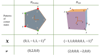
Figure S1: The two systems are shaped as a regular pentagon and a cube, respectively. The Bott indices $\boldsymbol{\nu}$ and configuration vectors $\boldsymbol{\chi}$ of these systems adhere to the analytical relationship outlined in the main text. For $H_{penta}$, the system size $L$ is $30$, and for $H_{3D}$, it is $15$.

Second, we examine a model with a cubic shape.

$$h_{3D}(\boldsymbol{k})= (m_{x}-i\gamma_{x}\sin k_{x})\mathbbm{1}+(t_{z}+\gamma_{z}\cos k_{z})\tau_{x}\otimes\tau_{0}-\gamma_{z}\sin k_{z}\tau_{y}\otimes\tau_{0}$$ (S42)

$$-(t_{y}-\gamma_{y}\cos k_{y})\tau_{z}\otimes\tau_{x}+\gamma_{y}\sin k_{y}\tau_{x}\otimes\tau_{y}+(t_{x}+\gamma_{x}\cos k_{x})\tau_{z}\otimes\tau_{z}.$$

All possible patterns of HOTPs in this system can be captured by Bott indices, defined by the following $f/g$,

$$\{\frac{4XYZ}{L^{3}},\frac{2XY}{L^{2}},\frac{2XZ}{L^{2}},\frac{2YZ}{L^{2}},\frac{X}{L},\frac{Y}{L},\frac{Z}{L}\}$$ (S43)

with

$$\mathcal{M}=\frac{1}{2}\begin{pmatrix}-1&1&-1&1&1&-1&1&-1\\ 1&-1&1&-1&1&-1&1&-1\\ -1&1&1&-1&1&-1&-1&1\\ -1&-1&1&1&1&1&-1&-1\\ 1&-1&-1&1&1&-1&-1&1\\ 1&1&-1&-1&1&1&-1&-1\\ -1&-1&-1&-1&1&1&1&1\\ 1&1&1&1&1&1&1&1\\ \end{pmatrix}.$$ (S44)

For example, when $m_{x}=0.7$, $t_{x}=0.1$, $\gamma_{x}=0.8$, $t_{y}=t_{z}=0$, $\gamma_{y}=\gamma_{z}=1$, this system exhibits a HOTP with the configuration vector $\boldsymbol{\chi}_{8}=(-1,1,0,0,0,0,1,-1)$. As shown in Fig. S1, the series of Bott indices equals $(2,0,0,0,-2,0,0)$, demonstrating that HOTPs can be fully characterized by

$$\boldsymbol{\chi}_{8}=\mathcal{M}^{-1}\cdot\left(\nu^{(1)}_{8},\dots,\nu^{(7)}_{8},0\right)^{\mathrm{T}}.$$ (S45)

VI Quadrupole Moment $q_{xy}$ and Multipole Chiral Number $N_{xy}$ in real space

VI.1 Definitions

In this section, we provide the definitions of $q_{xy}$ and $N_{xy}$ used in our calculations of Fig. 2(a) of the main text.

The quadrupole moment defined in the real space is given by [42, 43, 44]:

$$q_{xy}=\frac{1}{2\pi}\operatorname{Im}\log\left[\operatorname{det}\left(V^{\dagger}\hat{Q}V\right)\sqrt{\operatorname{det}\left(\hat{Q}^{\dagger}\right)}\right]\quad\operatorname{mod}1.$$ (S46)

$V$ is a matrix composed of all the occupied eigenstates of $H$ under periodic boundary conditions. $\hat{Q}=e^{2\pi i\frac{XY}{L^{2}}}$.

Multipole chiral number, defined in 2D systems, is given by [28]:

$$N_{xy}=\frac{1}{2\pi i}\operatorname{Tr}\operatorname{Log}\left(V_{A}^{\dagger}\hat{Q}^{c}V_{A}V_{B}^{\dagger}\hat{Q}^{c\dagger}V_{B}\right),$$ (S47)

where $V_{A}$ and $V_{B}$ is determined by the singular value decomposition of $h$, $h=V_{A}\Sigma V_{B}^{\dagger}$, under the periodic boundary condition. $\hat{Q}^{c}=e^{2\pi i\frac{XY}{L^{2}}}$, with position operators represented in the subspace of chiral operator.

VI.2 The relationship between $q_{xy}$ and $N_{xy}$

In this section, we prove the correspondence between $q_{xy}$ and $N_{xy}$ in chiral-symmetric systems,

$$q_{xy}=\frac{N_{xy}}{2}\quad\operatorname{mod}1.$$ (S48)

Since the following derivations do not contain the information of multipole operator, the conclusion can be generalized to higher multipole situations.

Taking the eigenbasis of chiral operator, we rewrite $V$ in $q_{xy}$ as:

$$V=\frac{1}{\sqrt{2}}\begin{pmatrix}V_{A}\\ V_{B}\end{pmatrix},$$ (S49)

and rewrite $\hat{Q}$ in $q_{xy}$ as:

$$\hat{Q}=\begin{pmatrix}\hat{Q}^{c}&0\\ 0&\hat{Q}^{c}\end{pmatrix}.$$ (S50)

Therefore, we have:

$$q_{xy} =\frac{1}{2\pi}\operatorname{Im}\log\left[\operatorname{det}\left(V^{\dagger}\hat{Q}V\right)\sqrt{\operatorname{det}\left(\hat{Q}^{\dagger}\right)}\right]\quad\operatorname{mod}1$$ (S51)

$$=\frac{1}{2\pi}\operatorname{Im}\log\left[\operatorname{det}\left(V_{A}^{\dagger}\hat{Q}^{c}V_{A}+V_{B}^{\dagger}\hat{Q}^{c}V_{B}\right)\sqrt{\operatorname{det}\left(\hat{Q}^{\dagger}\right)}\right]\quad\operatorname{mod}1$$

$$=\frac{1}{2\pi}\operatorname{Im}\log\left[\operatorname{det}\left(V_{A}^{\dagger}\hat{Q}^{c}V_{A}V_{B}^{\dagger}\hat{Q}^{c\dagger}V_{B}+\mathbbm{1}\right)\right]\quad\operatorname{mod}1,$$

where in the last step we use $\operatorname{det}\left(\hat{Q}^{c}\right)\sqrt{\operatorname{det}\left(\hat{Q}^{\dagger}\right)}=1$.

Denoting the eigenvalues of $V_{A}^{\dagger}\hat{Q}^{c}V_{A}V_{B}^{\dagger}\hat{Q}^{c\dagger}V_{B}$ as $e^{i\lambda_{i}}$, we have

$$N_{xy}=\frac{1}{2\pi i}\operatorname{Tr}\operatorname{Log}\left(V_{A}^{\dagger}\hat{Q}^{c}V_{A}V_{B}^{\dagger}\hat{Q}^{c\dagger}V_{B}\right)=\frac{\sum_{i}\lambda_{i}}{2\pi}.$$ (S52)

We express the $q_{xy}$ as follows:

$$q_{xy} =\frac{1}{2\pi}\operatorname{Im}\log\left[\operatorname{det}\left(V_{A}^{\dagger}\hat{Q}^{c}V_{A}V_{B}^{\dagger}\hat{Q}^{c\dagger}V_{B}+\mathbbm{1}\right)\right]\quad\operatorname{mod}1$$ (S53)

$$=\frac{1}{2\pi}\operatorname{Im}\log\left[\prod_{i}\left(e^{i\lambda_{i}}+1\right)\right]\quad\operatorname{mod}1$$

$$=\frac{1}{2\pi}\operatorname{Im}\sum_{i}\log\left(e^{i\lambda_{i}}+1\right)\quad\operatorname{mod}1$$

$$=\frac{1}{2\pi}\operatorname{Im}\sum_{i}i\frac{\lambda_{i}}{2}\quad\operatorname{mod}1$$

$$=\frac{\sum_{i}\lambda_{i}}{4\pi}\quad\operatorname{mod}1$$

$$=\frac{N_{xy}}{2}\quad\operatorname{mod}1.$$

VI.3 Discussions

Generally, both $N_{xy}$ and $q_{xy}$ are defined in systems with rectangular shapes. The form of $N_{xy}$ suggests a structural similarity to the Bott index $\nu$, as defined in the main text. As shown by the definition of $N_{xy}$, it can be rewritten in the form of the Bott index,

$$N_{xy}=\operatorname{Bott}\left(\hat{Q}^{c},V_{A}V_{B}^{\dagger}\right).$$ (S54)

It should be noted that under periodic boundary conditions, the Bott index form of $N_{xy}$ may be ill-defined according to the Definition I.1, with $\parallel[\hat{Q}^{c},V_{A}V_{B}^{\dagger}]\parallel$ equaling $2$. This is because the hopping, required by periodic boundary condition, is long-ranged, which renders Theorem I.2 inapplicable to Hamiltonians under such conditions. Let us illustrate this by considering

$$e^{2\pi i\frac{x_{m}y_{m}-x_{n}y_{n}}{L^{2}}},$$

which appears in the proof of Theorem I.2, Eq. (S10), when $f/g=XY/L^{2}$. Choosing $x_{m}=1$, $x_{n}=L-R$, and $y_{m}=y_{n}=L/2$, we have

$$e^{2\pi i\frac{x_{m}y_{m}-x_{n}y_{n}}{L^{2}}}=-1,$$

when $R\ll L$. Thus, Eq. (S10) in the proof of Theorem I.2 is not satisfied. There is no lower bound for $\parallel[\hat{Q}^{c},V_{A}V_{B}^{\dagger}]\parallel$, even in the limit of large system size.