An evaluation of the BALROG and RoboBA algorithms for determining the position of Fermi/GBM GRBs

Abstract

The Fermi/GBM instrument is a vital source of detections of gamma-ray bursts and has an increasingly important role to play in understanding gravitational-wave transients. In both cases, its impact is increased by accurate positions with reliable uncertainties. We evaluate the RoboBA and BALROG algorithms for determining the position of gamma-ray bursts detected by the Fermi/GBM instrument. We construct a sample of 54 bursts with detections both by Swift/BAT and by Fermi/GBM. We then compare the positions predicted by RoboBA and BALROG with the positions measured by BAT, which we can assume to be the true position. We find that RoboBA and BALROG are similarly precise for bright bursts whose uncertainties are dominated by systematic errors, but RoboBA performs better for faint bursts whose uncertainties are dominated by statistical noise. We further find that the uncertainties in the positions predicted by RoboBA are consistent with the distribution of position errors, whereas BALROG seems to be underestimating the uncertainties by a factor of about two. Additionally, we consider the implications of these results for the follow-up of the optical afterglows of Fermi/GBM bursts. In particular, for the DDOTI wide-field imager we conclude that a single pointing is best. Our sample would allow a similar study to be carried out for other telescopes.

1 Introduction

Gamma-ray bursts (GRBs) are transient events with isotropic energies of $10^{50}$–$10^{53}$ ergs caused by a collimated relativistic jet launched from the vicinity of a compact central engine (Gehrels & Razzaque, 2013). They consist of an initial prompt emission of gamma-ray photons, largely from internal shocks in the jet, followed by an afterglow at longer wavelengths resulting from the interaction of the jet with the circumstellar medium (Sari et al., 1998; Granot & Sari, 2002).

GRBs are empirically classified into two populations using the time interval $T_{90}$ between the moments at which $5\%$ and $95\%$ of the prompt emission are detected (Kouveliotou et al., 1993). GRBs are classified as short (SGRB) if they have a $T_{90}<2$ s and long (LGRB) if they have a $T_{90}>2$ s. This classification is important as there is a strong correlation between $T_{90}$ and the progenitor system. LGRBs tend to be the result of the death of massive stars following core collapse (Woosley, 1993; Woosley & Bloom, 2006), whereas SGRB tend to arise from the merger of compact binary systems with at least one neutron star (Lee & Ramirez-Ruiz, 2007; Abbott et al., 2017; Eichler et al., 1989; Narayan et al., 1992; Ruffert & Janka, 1998). These mergers are caused by the orbital decay of the compact binary system due to the emission of gravitational radiation, and as such are important for multi-messenger astronomy (Branchesi, 2016). The two populations do overlap to some degree, and so there is ambiguity when $T_{90}$ is around 2 s (Dimple et al., 2022; Garcia-Cifuentes et al., 2024; Yang et al., 2022; Troja et al., 2022).

For many reasons, the afterglow phase is vitally important for the identification and subsequent follow-up of GRBs. Gamma-ray detectors tend to have poor angular resolution, so observations of the afterglow in X-rays or the optical are the best means to obtain a localization at the level of arcseconds. Such localizations allow us to tie a GRB to its host galaxy or conversely demonstrate that it occurs outside of a galaxy. They are also necessary for redshift determination, which to date have been made either directly from the afterglow or from the host galaxy associated with the afterglow. Finally, the afterglow provides important information on the environment in which the GRB occurred.

The Swift satellite (Gehrels et al., 2004) has allowed us to exploit these characteristics of GRBs and their afterglows over the last 19 years. GRBs are detected in gamma rays by the BAT instrument (Barthelmy et al., 2005), and then the afterglow is localized to arcsec-precision in X-rays by the XRT (Burrows et al., 2005; Evans et al., 2009) and in the optical by UVOT (Roming et al., 2005, 2017; Page et al., 2019). The main disadvantages of Swift are the relatively small field-of-view of BAT of about 1.4 sr (only about 11% of the sky), the relatively soft response of BAT (up to about 150 keV), and worries about its longevity given its age and reliance on reaction wheels (Cenko, 2022).

The Fermi satellite has several advantages compared to Swift. Its GBM instrument views 70% of the sky and has good sensitivity up to 10 MeV (Meegan et al., 2009). These properties allow it to detect about 250 GRBs per year (von Kienlin et al., 2020), compared to about 100 for BAT (Lien et al., 2016). Furthermore, its response at higher energies allows it to detect about 40 SGRBs per year (Kocevski et al., 2018), whereas BAT detects only about 10 (Lien et al., 2014). On the other hand, the localizations delivered by GBM have typical uncertainties of 5–15 deg (Connaughton et al., 2015), and Fermi is not equipped with a means to improve this by observing emission from the afterglow. Some GBM GRBs are also detected at higher energies by the LAT instrument and localized to about 10 arcmin, but only about 20 per year (Ajello et al., 2019).

Instead, precise localizations of GBM GRBs must typically be provided by the detection of the optical afterglow by wide-field imagers such as iPTF (Singer et al., 2015), DDOTI (Watson et al., 2016), GOTO (Mong et al., 2021), and ZTF (Ahumada et al., 2022). The success of these searches is improved by having not only good estimates of the positions from GBM but also good estimates of the uncertainties in these positions.

Moreover, GBM has acquired new importance in the era of gravitational-wave astronomy, as its wide field gives an excellent chance of detecting faint gamma-ray emission associated with nearby gravitational-wave sources such as compact binary mergers. This was dramatically demonstrated in the case of GRB 170817A, which was produced by GW170817 (Abbott et al., 2017; Goldstein et al., 2017; Savchenko et al., 2017). Detections by GBM allow the search area to be narrowed and provide vital information on the nature of the progenitors and remnant. One such a system is RAVEN adopted by the LVK collaboration (Adhikari et al., 2023; Sharma Chaudhary et al., 2023).

For these reasons, accurate positions and reliable uncertainties for GBM detections are increasingly important. In this work, we evaluate two current systems that estimate the position of GBM GRBs: the RoboBA system (Connaughton et al., 2015; Goldstein et al., 2020) and the BALROG system (Burgess et al., 2018; Berlato et al., 2019). In contrast to previous work, we will use published positions produced by the teams behind both systems. Thus, our evaluation is entirely empirical and independent.

Our paper is organized as follows. In section 2 we briefly describe the GBM instrument and the means by which it provides information for localizing GRBs. In section 3 we describe the products of the RoboBA and BALROG processes. In section 4 we describe the samples we use to evaluate the performance of RoboBA and BALROG. In section 5 we consider the accuracy of both the position estimates and the uncertainty estimates. In section 6 we determine the most appropriate observation strategy for our wide-field imager DDOTI based on our results. Finally, in section 7 we summarize and discuss our results.

2 GBM Positions

Fermi/GBM has twelve sodium iodide (NaI) detectors sensitive over an energy range from 8 keV to 1 MeV and two bismuth germanate (BGO) scintillators sensitive from 200 keV to 40 MeV (Meegan et al., 2009). The NaI detectors are distributed around the spacecraft and oriented in different directions. The two BGO detectors are on opposite sides of the spacecraft. The signal measured in each detector depends on the position and spectrum of the source for two main reasons: each detector has an energy-dependent angular response function, and absorption in the spacecraft reduces the count rate in detectors on the side that faces away from the source. In addition, the scattering of gamma rays from the Earth’s atmosphere also changes the relative count rates. By modeling the count rates, taking into account the spectrum of the source, the position can be determined, albeit with significant uncertainties.

The Fermi spacecraft provides initial “flight” positions calculated by an on-board computer. While these are produced in 10––30 s (Connaughton et al., 2015), the meager processing power available limits their accuracy. Better “ground” positions are provided by subsequent processing of downloaded data using more powerful computers on the Earth.

In the first years of the Fermi mission, ground positions were provided by having the Burst Advocates manually run the Daughter of Location (DoL) algorithm (Connaughton et al., 2015). This algorithm fits the count rates by varying the position of the source and allowing it to have one of three different spectra representing soft, medium, and hard GRBs. In their evaluation of DoL, Connaughton et al. (2015) found that the statistical uncertainties for bright GRBs could be as small as 1 deg, but the systematic uncertainties were well represented by a Gaussian with $1\sigma$ radius of 3.7 degrees and a non-Gaussian tail containing about 10% of the probability and extending to approximately 14 deg.

The BALROG algorithm was created by Burgess et al. (2018). The major advance was noting that there were correlations between the position and spectrum of the GRB, and so in theory a better determination of the uncertainties could be obtained by fitting simultaneously for both. This could also reduce the apparent systematic error in the determination of the position of bright GRBs. The original BALROG algorithm was improved and automated by Berlato et al. (2019), and produces positions in a matter of minutes, although the delay before the GBM data is publically released is an important factor. The BALROG algorithm is specifically tuned for bright GRBs; for example, it uses only about 10 seconds of data, to avoid smearing in the response caused by the motion of the spacecraft. Berlato et al. (2019) also compared the BALROG results to DoL and found that BALROG gave more precise positions, at least for bright GRBs in which the DoL uncertainty is dominated by systematic effects.

Subsequently, the RoboBA system was deployed. Goldstein et al. (2020) describe it as an automated system that uses an improved version of the earlier Daughter of Location (DoL) and report that the systematic uncertainty for the updated RoboBA localizations was 1.8 degrees for 52% of GRBs and 4.1 for the remaining 48%. RoboBA also runs in a matter of minutes and has the advantage of early access to proprietary GBM data. Goldstein et al. (2020) compared the RoboBA results to BALROG, and found that RoboBA gave more precise positions.

Both systems distribute their results in a form that is convenient for robotic telescopes. The GBM flight positions and RoboBA positions are distributed using GCN Notices (Barthelmy et al., 1998). The BALROG positions are distributed as JSON and FITS files whose locations can be derived from the GBM trigger number. In this sense, there is little to choose between the two. (The BALROG team also send GCN Circulars, but it is more difficult for a robotic system to automatically extract information from the text in these.)

Our direct interest in GBM positions is to use them to point our wide-field imager DDOTI (Watson et al., 2016). In the first few minutes after a burst we only have GBM flight positions and RoboBA positions. After this initial period, we have both BALROG and RoboBA positions, and obviously we wish to use the better one. This requires understanding the performance of each algorithm. The situation we faced at the start of this work was that each team had published results that indicated that their approach gave better positions. Therefore, we embarked on this independent empirical study to gain a clearer understanding of the matter.

3 Position Estimations and Uncertainties

In this section, we briefly describe the products of the RoboBA and BALROG algorithms and in particular their model uncertainties. This is useful to establish our notation.

Each algorithm provides estimators $\hat{\alpha}$ and $\hat{\delta}$ of the true right ascension $\alpha$ and declination $\delta$ of the burst. We will use $\gamma$ to be the total angular distance error (i.e., the angular distance between the estimated position and the true position) and $\gamma_{\alpha}$ and $\gamma_{\delta}$ to be the corresponding angular distances parallel to the local right ascension and declination axes.

One potentially confusing aspect is that the error distributions are traditionally described in terms of the circle or ellipse corresponding to $1\sigma$, $2\sigma$, or $3\sigma$ (Briggs et al., 1999; Connaughton et al., 2015; Berlato et al., 2019). This does not mean that the angular radius of the circle is that number of standard deviations. Rather, it means that the probability within the circle or ellipse is the same as that within $\pm 1\sigma$, $\pm 2\sigma$, and $\pm 3\sigma$ of a one-dimensional Gaussian distribution, that is, 0.6827, 0.9545, and 0.9973.

For a two-dimensional circular Gaussian distribution with standard deviation $a$ in each coordinate, the probability density is

$$p(\gamma)=\frac{1}{2\pi a^{2}}e^{-\gamma^{2}/2a^{2}}.$$ (1)

We can easily integrate this and find that the $1\sigma$, $2\sigma$, and $3\sigma$ radii correspond to $\gamma=1.515a$, $2.486a$, and $3.439a$.

3.1 RoboBA

RoboBA uses the “DoL” algorithm described in detail by Connaughton et al. (2015) and Goldstein et al. (2020).

The model error distribution is based on the von Mises-Fisher distribution (Fisher et al., 1987; Briggs et al., 1999; Connaughton et al., 2015), which is a generalization of the Gaussian distribution to the surface of a sphere, and is given by

$$p(\gamma)=\frac{\kappa}{2\pi\left(e^{\kappa}-e^{-\kappa}\right)}e^{\kappa\cos\gamma},$$ (2)

in which the concentration parameter $\kappa$ is used to characterize the width of the distribution. The probability within an angular radius $\gamma$ is

$$P(\leq\gamma)=\frac{\kappa}{2\pi\left(1-e^{-2\kappa}\right)}\int_{\Omega}e^{\kappa(\cos\gamma-1)}\,d\Omega.$$ (3)

Unfortunately, this integral does not, in general, have a closed form. Therefore, to advance, we rewrite the distribution as

$$p(\gamma)=\frac{\kappa}{2\pi(1-e^{-2\kappa})}e^{\kappa(\cos\gamma-1)}.$$ (4)

This form has two advantages in our current context in which $\gamma$ is typically small and $\kappa$ is typically large. First, this form avoids overflow when evaluated numerically. Second, we can approximate $\cos\gamma$ as $1-\gamma^{2}/2$ with an error of less than 1 part in 1000 out to a radius of 20 deg, and substituting this into equation (4) we rapidly obtain an approximate Gaussian distribution,

$$p(\gamma)\approx\frac{\kappa}{2\pi}e^{-\kappa\gamma^{2}/2}.$$ (5)

We can then use all of the standard results for a Gaussian. Comparing equations 1 and 5, we see that $\kappa^{-1}\approx a^{2}$ and so in terms of the $1\sigma$ angular radius $\sigma$ in radians (Briggs et al., 1999),

$$\kappa^{-1}\approx 0.660^{2}\sigma^{2}.$$ (6)

The numerical factor here is simply the inverse of the factor 1.515 in the relation between $\sigma$ and $a$ derived above. When $\sigma\leq 10$ deg (i.e., $\sigma\leq 0.18$ rad), $\kappa\geq 75$, which validates our assumption that $\kappa$ is typically large.

The DoL algorithm uses two von Mises-Fisher distributions, one for the core (containing a fraction $f$ of the probability), and one for the tail (Connaughton et al., 2015; Goldstein et al., 2020). That is, the probability that the error is less than the angular distance $\gamma$ is given by

$$P(\leq\gamma)=fP_{\mathrm{core}}(\leq\gamma)+(1-f)P_{\mathrm{tail}}(\leq\gamma).$$ (7)

The two distributions $P_{\mathrm{core}}$ and $P_{\mathrm{tail}}$ are von Mises-Fisher distributions with different values of the concentration parameter $\kappa_{\mathrm{core}}$ and $\kappa_{\mathrm{tail}}$. Each combines the statistical uncertainty $\sigma_{\mathrm{stat}}$ with different values of the systematic uncertainty $\sigma_{\mathrm{sys}}$. For $P_{\mathrm{core}}$, we have

$$\kappa_{\mathrm{core}}^{-1}=0.660^{2}(\sigma_{\mathrm{stat}}^{2}+\sigma_{\mathrm{core}}^{2}),$$ (8)

whereas for $P_{\mathrm{tail}}$, we have

$$\kappa_{\mathrm{tail}}^{-1}=0.660^{2}(\sigma_{\mathrm{stat}}^{2}+\sigma_{\mathrm{tail}}^{2}).$$ (9)

The statistical uncertainty $\sigma_{\mathrm{stat}}$ is distributed with the predicted position. To calculate the model error distribution, we also need the fraction of probability in the core and the systematic uncertainties for the two components. We adopt the “Updated RoboBA All GRBs” model of Goldstein et al. (2020), which has $f=0.517$, $\sigma_{\mathrm{core}}=1.81~{}\mathrm{deg}$, and $\sigma_{\mathrm{tail}}=4.07~{}\mathrm{deg}$.

3.2 BALROG

The BALROG algorithm produces two-dimensional images of the probability distribution of the position on the sky (Burgess et al., 2018). Two images are produced for each localization, one with just the statistical uncertainty and another convolved with a two-dimensional Gaussian representing the systematic uncertainty (Berlato et al., 2019). The BALROG team view these images as their primary products (Greiner, private communiation).

Subsequently, the BALROG process fits the unconvolved image with a two-dimensional Gaussian,

$$p(\gamma_{\alpha},\gamma_{\delta})=\frac{1}{2\pi a_{\alpha}a_{\delta}}e^{-(\gamma_{\alpha}^{2}/a_{\alpha}^{2}+\gamma_{\delta}^{2}/a_{\delta}^{2})/2}.$$ (10)

in which $\gamma_{\alpha}$ and $\gamma_{\delta}$ are the angular separations in $\alpha$ and $\delta$ and $a_{\alpha}$ and $a_{\delta}$ are the corresponding standard deviations (Berlato et al., 2019). The results of the fit are given as $\sigma_{\alpha}$ and $\sigma_{\delta}$, the half-axes of the ellipse that contains 0.683 of the probability. Note that $\sigma_{\delta}$ is given in terms of $\alpha$, not the separation $\gamma_{\alpha}$, and so needs to be multiplied by $\cos\hat{\delta}$ before being used with angular separations. The systematic uncertainty $\sigma_{\mathrm{sys}}$ is also given as the radius enclosing 0.683 of the probability and is typically 1.0 or 2.0 deg. All of these parameters are distributed as secondary products by the BALROG team.

To obtain an approximation of the parameters $\sigma_{\alpha}^{\prime}$ and $\sigma_{\delta}^{\prime}$ of an equivalent fit to the image after convolution with the systematic uncertainty, we add the systematic uncertainty in quadrature as follows,

$$(\sigma_{\alpha}^{\prime}\cos\delta)^{2}=(\sigma_{\alpha}\cos\delta)^{2}+(\sigma_{\mathrm{sys}})^{2}$$ (11)

and

$$(\sigma_{\delta}^{\prime})^{2}=(\sigma_{\delta})^{2}+(\sigma_{\mathrm{sys}})^{2}.$$ (12)

The final Gaussian then has

$$a_{\alpha}=0.660\sigma_{\alpha}^{\prime}\cos\delta$$ (13)

and

$$a_{\delta}=0.660\sigma_{\delta}^{\prime}.$$ (14)

Using the transformations $\gamma_{\alpha}=r\cos\theta$ and $\gamma_{\delta}=(a_{\delta}^{\prime}/a_{\alpha}^{\prime})r\sin\theta$, we can show that the probability contained within an equiprobability ellipse that passes through a point with separations $\gamma_{\alpha}$ and $\gamma_{\delta}$ is

$$P(\gamma_{\alpha},\gamma_{\delta})=1-e^{-\left[(\gamma_{\alpha}/a_{\alpha}^{\prime})^{2}+(\gamma_{\delta}/a_{\delta}^{\prime})^{2}\right]/2}.$$ (15)

In our analysis below, we will use both the two-dimensional images (including systematic errors) and equation (15). Both give very similar results, which validates our approach to incorporating the systematic errors into the BALROG fits.

4 Samples

We evaluate the two algorithms using a full sample of 54 GRBs detected by both Fermi/GBM and Swift/BAT and with published positions from BAT, RoboBA, and BALROG and using a bright subsample of 27 GRBs. In this section, we describe the construction of the samples.

4.1 Full Sample

We first generated a list of all of the GRBs detected by GBM between 2019 September 14 UTC and 2023 November 07 UTC. The start date was chosen to be when version 41731 of the RoboBA ground software started to be used (for trigger 590141799 corresponding to GRB 190914.345). The end date has no particular external significance but was when we began the final analysis for publication. This interval excludes the GRBs used to calibrate the two algorithms. To create the list, we examined the GCN Notices distributed by the GBM team and ignored triggers that did not have “GRB” as the MOST_LIKELY classification value in the latest notice (e.g., GRB 220826497 was initially classified as most likely to be distant particles, but subsequently reclassified as most likely to be a GRB). This gave a list of 984 GRBs.

We then generated a list of all GRBs detected by BAT in the same interval from the “Swift Trigger and Burst Real-Time Information” table on the GCN website. This gave a list of 398 GRBs.

We matched the two lists under the assumption that GRBs that have trigger times within 100 seconds are the same. This gave a list of 74 GRBs detected by both GBM and BAT. Since these events were detected by both satellites, there is a strong likelihood that they are real astrophysical bursts.

We then matched the GBM bursts with the BALROG positions in the “GBM-Locations” catalog on the MPE website. We found positions for 54 of the 74 GRBs and found one other (GRB 200427768) for which the BALROG analysis was noted as having failed. We do not know why there are no BALROG positions for the other 19 GRBs. While some are faint, others are bright enough to have small RoboBA statistical uncertainty. We do not use these 20 GRBs in our analysis, but only the 54 for which published positions from both RoboBA and BALROG are available. These 54 GRBs form our full sample.

Table 1 shows the list of 74 GRBs detected by both GBM and BAT. The first column shows the GBM GRB name (year, month, day, and thousandths of a day) and the next two columns show the BAT and GBM trigger numbers. After that, the table shows the positions from BAT, RoboBA, and BALROG. The uncertainties on the BAT positions are typically 3 arcmin in radius (90% probability) and are negligible compared to the uncertainties of at least 1 deg in the position estimates from both RoboBA and BALROG. Therefore, we take the BAT positions to be the true position $\alpha$ and $\delta$. For RoboBA we show the version of the software, the estimated position $\hat{\alpha}$ and $\hat{\delta}$, and the statistical uncertainty $\sigma_{\mathrm{stat}}$ defined in section 3.1. For BALROG, we show the estimated position $\hat{\alpha}$ and $\hat{\delta}$, the statistical uncertainties $\sigma_{\alpha}$ and $\sigma_{\beta}$, and the systematic uncertainty $\sigma_{\mathrm{sys}}$, defined in section 3.2.

Most of the RoboBA positions are ground positions produced by version 41731 of the software, but a few are flight positions produced by version 3 or ground positions produced by versions 415 or 4173.

Table 3 shows derived quantities for the full sample of 54 GRBs used in the analysis. In particular, it shows the error $\gamma$ in deg between the positions estimated by RoboBA and BALROG and the true position determined by BAT.

4.2 Bright Subsample

Our full sample includes both bright and faint GRBs and as such is in some ways unfair to BALROG, which is optimized to give improved positions of the brightest GRBs. For example, the current implement of BALROG uses only 10 seconds of data around the peak to avoid smearing due to the motion of the spacecraft (Berlato et al., 2019), whereas our understanding is that RoboBA uses a longer interval and so might be expected to give better results for fainter GRBs dominated by statistical errors.

The question of whether a GRB is bright in this sense is not completely clearly defined. One might consider only GRBs with $T_{90}$ of no more than 10 seconds, so that BALROG sees almost all of the flux, or consider the peak flux. However, we have adopted an empirical approach; essentially, we ask BALROG if it considers a GRB to be well-localized or not according to the statistical uncertainty, which is indirectly related to the number of photons analysed by BALROG. For each GRB, we determine the equivalent BALROG circular statistical uncertainty $\sigma$ using

$$\sigma^{2}\equiv(\sigma_{\alpha}\cos\delta)(\sigma_{\delta}).$$ (16)

Table 3 shows $\sigma$ in deg for each GRB. We then define a bright subsample of 27 GRBs that includes only those GRBs with equivalent circular uncertainties smaller than the median of $5.7~{}\deg$.

4.3 BALROG Map Subsample

The BALROG “GBM-Locations” catalog on the MPE website also contains FITS HEALPIX images containing the probability distribution on the sky. Unfortunately, we were only able to find images for the 25 GRBs from GRB 210211363 and later. We refer to these 25 as the BALROG map subsample. Furthermore, 12 are also in our bright subsample and so form the bright BALROG map subsample.

5 Analysis

5.1 Distribution of Errors

We first consider the distribution of the errors in the position. For each GRB in our sample, we determined the error as the angular distance $\gamma$ between the BAT position, which is assumed to be the true position, and the positions estimated by the RoboBA and BALROG algorithms.

Figure 1 a shows the cumulative distribution of errors for both algorithms and for the full sample of 54 GRBs. We see that the two algorithms give very similar results for the roughly 25% of GRBs with errors of up to about 3 degrees, but after that, the RoboBA algorithm has smaller errors than the BALROG algorithm. The median errors, shown with dashed lines in Figure 1a, are $3.7~{}\deg$ for RoboBA and $9.2~{}\deg$ for BALROG.

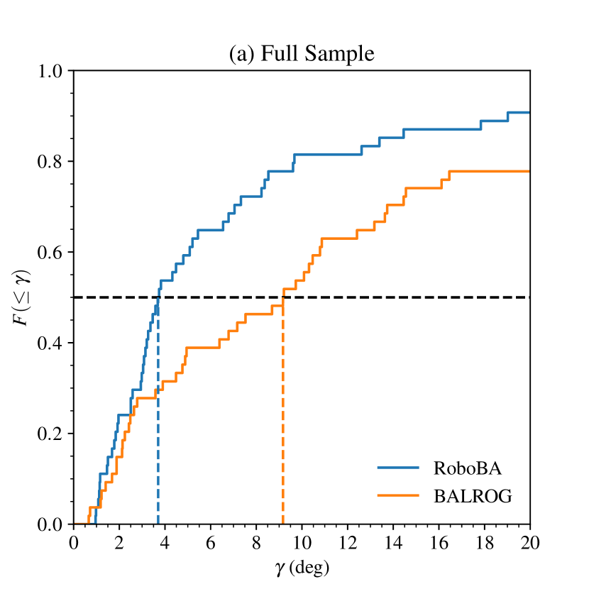
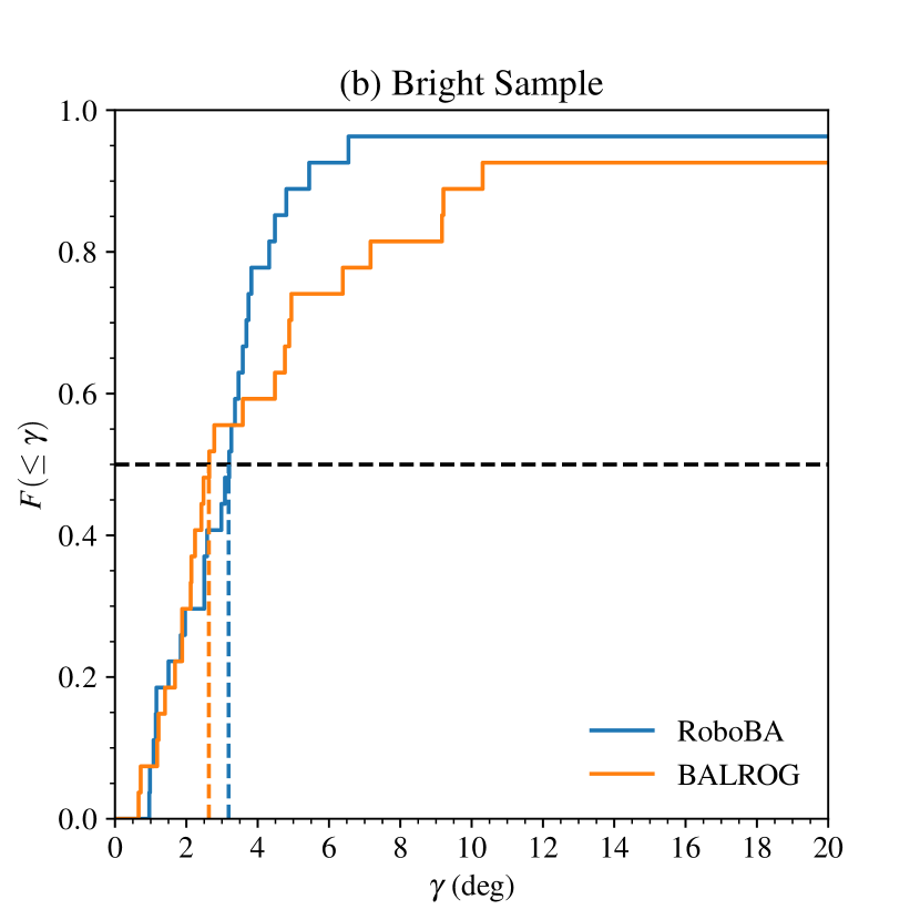
Figure 1: The cumulative distribution of position errors $\gamma$ for the RoboBA and BALROG algorithms for the GRBs in (a) the full sample (above) and (b) the bright subsample (below). The median errors, shown with dashed lines, are 3.7 and $3.2~{}\deg$ for RoboBA and 9.2 and $2.6~{}\deg$ for BALROG.

Figure 1b shows the cumulative distribution of errors for both algorithms and for the bright subsample. The results are now quite different. The two algorithms give very similar results for the better-localized half of the subsample. The median errors, shown with dashed lines in Figure 1b, are $3.2~{}\deg$ for RoboBA and $2.6~{}\deg$ for BALROG.

The distributions suggest that BALROG is performing similarly or perhaps slightly better than RoboBA for the roughly 25% of brightest and best-localized GRBs. For the fainter and more poorly localized GRBs, RoboBA gives positions with smaller errors. This change in behavior is consistent with the stated optimization of BALROG for brighter GRBs (Berlato et al., 2019). We considered carrying out statistical tests on these samples to quantify these statements further. However, with so few GRBs in our samples, we are susceptible to large statistical fluctuations and also to somewhat arbitrary decisions (e.g., our choice of the median uncertainty to define the bright subsample, rather than a smaller or larger percentile , such as the bright subsample being those with uncertainties in the lowest 25%).

One feature that jumps out at us is that even in the bright subsample there are two BALROG positions (GRBs 220118764 and 220714582) and one RoboBA position (GRB 191011192) with errors of more than 60 deg. This gives some idea of the difficulties both groups have faced in finding a robust algorithm.

5.2 Distribution of Enclosed Probabilities

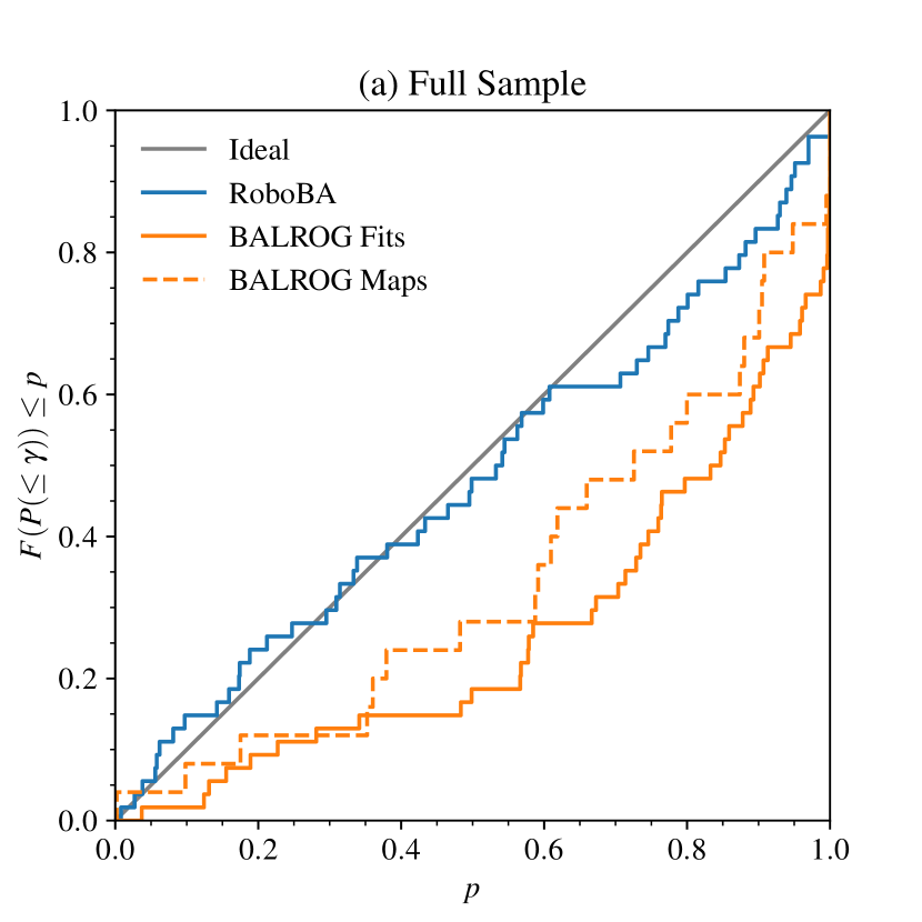
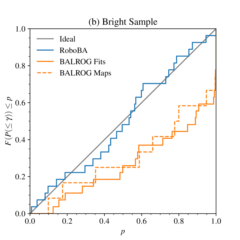
Figure 2: The cumulative distribution of enclosed probabilities for the RoboBA and BALROG algorithms for the GRBs in (a) the full sample (above) and (b) the bright subsample (below). For BALROG, the solid lines are determined from the Gaussian fits and the dashed lines are determined directly from the probability maps.

In addition to positions, both RoboBA and BALROG distribute estimates of the uncertainties in the position. It is important to understand how well these estimates reflect reality. In an ideal case, the cumulative distribution of probability enclosed within the observed offset $\gamma$ should be a straight line from 0 to 1. In the case of RoboBA, the enclosed probability is given by equation (7). In the case of BALROG, we determined it in two ways. For the full sample, we used equation (15) to determine the probability within the equiprobability ellipse passing through the true position. For the map subsample, we directly summed the probability in the maps (the ones that explicitly include the systematic error) within a circle centered on the estimated position and whose radius was the angular distance to the true position. Table 3 gives these three probabilities.

The cumulative distributions of enclosed probability are shown in Figure 2a for the whole sample and Figure 2b for the bright subsample. For BALROG, we show two determinations: the solid lines are determined from the Gaussian fits and the dashed lines are determined directly from the probability maps.

We see that the line for RoboBA is quite close to the ideal case, both for the full sample and the bright subsample. This suggests that the uncertainties are accurately given by RoboBA. On the other hand, the lines for BALROG are dramatically below the ideal for both samples and for both probabilities determined from the fits and from the maps. This strongly suggests the true uncertainties in the position are underestimated by BALROG.

In the full sample, the fraction of GRB errors within the estimated $1\sigma$ ($P=0.6827$) uncertainty region is 61% for RoboBA, 31% for BALROG with probabilities determined from the fits, and 48% for BALROG with probabilities determined from the maps. For the bright subsample, the corresponding percentages are 70% for RoboBA and 37% and 42% for BALROG.

Again, we need to remind ourselves that BALROG was optimized for bright GRBs (Berlato et al., 2019). Therefore, we should not be too demanding of its performance with the full sample, which includes both bright and faint GRBs. However, it is somewhat surprising that the cumulative distribution for the bright subsample differs so much from the ideal case.

To quantify the magnitude of the effect, we found that if we artificially increased the BALROG uncertainties from the fits by a factor of two, the percentage within the estimated $1\sigma$ ($P=0.6827$) uncertainty region rose from 37% to 63%. Thus, it appears that the uncertainties generated by BALROG are underestimated by roughly a factor of two.

6 Application to DDOTI

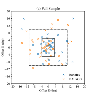
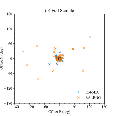
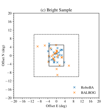
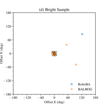
Figure 3: The errors in the positions shown relative to the DDOTI fields. The solid black rectangle represents one DDOTI field ($7\times 10$ deg). The dashed black rectangle represents a mosaic of $3\times 2$ DDOTI fields ($21\times 20$ deg). The crosses show the errors in the RoboBA and BALROG positions. The upper panels are for the full sample and the lower panels are for the bright subsample. The left panels zoom in on the DDOTI field. The right panels show the tail of outliers.

DDOTI is a wide-field imager installed at the Observatorio Astronómico Nacional on the Sierra de San Pedro Mártir in Baja California, Mexico (Watson et al., 2016). It consists of six 28 cm telescopes with prime-focus CCDs mounted on a common equatorial mount and offers an instantaneous field of view of approximately 70 $\mbox{deg}^{2}$ (7 deg E-W and 10 deg N-S) with a $10\sigma$ limited magnitude in 60 seconds of approximately $r\approx 18.7$ in dark time and $r\approx 18.0$ in bright time. Its main science goals are the localization and follow-up of optical transients associated with GRBs detected by Fermi/GBM and gravitational-wave events (Watson et al., 2020; Thakur et al., 2020; Becerra et al., 2021; Dichiara et al., 2021).

In its follow-up of GRBs detected by Fermi/GBM, DDOTI is a consumer of the estimated positions and uncertainties produced by the RoboBA and BALROG algorithms. At a practical level, we need to understand whether we should point the telescope using the RoboBA or BALROG positions and whether we should observe a single field or a larger mosaic. The second issue involves a trade-off between coverage and depth. DDOTI is typically background-limited and the optical transients fade rapidly, so if we observe at $N$ pointings we increase our effective field to about $70N$$\mbox{deg}^{2}$ but reduce our sensitivity by about $1.25\log N$ magnitudes. For mosaics with $1\times 1$, $2\times 1$, $2\times 2$, or $3\times 2$ pointings, we have fields of $7\times 10$, $14\times 10$, $14\times 20$ deg, and $21\times 20$ deg and corresponding losses of sensitivity of about 0.0, 0.4, 0.8, and 1.0 magnitudes.

To address these questions, we have simulated observations of our GRB samples with DDOTI. We assume that we center our single-field or mosaic either to the RoboBA or BALROG position, and then ask whether the BAT position would fall within a mosaic with a given size. Table 4 and Figure 3 shows the results. We see that centering the mosaic on the RoboBA position gives a higher fraction of GRBs within the field than centering the mosaic on the BALROG position. For example, if we choose to observe only one field, then pointing to the RoboBA position would give coverage at the true position of 57% of the full sample, whereas the same for the BALROG position would give only 35%. The corresponding percentages for the bright subsample are 81% for RoboBA and 67% for BALROG.

Considering the high fraction of GRBs within one field and the significant sensitivity loss for observing more than one pointing, our strategy for localizing GBM GRBs with DDOTI is to observe only a single pointing centered on the RoboBA position.

7 Conclusions

We have evaluated the precision of the estimates of GRB positions and the precision of the associated uncertainties for a sample of 54 GRBs detected by both Swift/BAT and Fermi/GBM and for which positions are available with recent versions of the RoboBA and BALROG algorithms.

We find that RoboBA and BALROG offer very similar results for approximately 25% of GRBs of bright GRBs with errors up to about 3 deg, RoboBA gives smaller errors beyond this range. This result was not entirely surprising, since BALROG was optimized for bright GRBs in which the systematic error can dominate (Berlato et al., 2019), and some of the improvements in RoboBA seem to have been stimulated by the earlier advances in BALROG. The approach taken by RoboBA minimizes the statistical error, which dominates for faint GRBs.

On the other hand, we find that while the uncertainties estimated by RoboBA correspond closely to the observed uncertainties, those produced by BALROG seem to underestimate the true uncertainties significantly, perhaps by a factor of two. This was an unexpected result. The uncertainties in the position of the GRB are important for defining the limits of the search area, both when determining the observing strategy and during subsequent analysis.

One of the advantages of BALROG, demonstrated by Burgess et al. (2018), is that it makes explicit the dependency between the source position and spectrum by solving for these simultaneously. Our results do not contradict this finding, as we focus only on the position. This suggests that it would be worthwhile to understand why the estimates of the positional uncertainties produced by BALROG seem to be underestimated, both to have confidence in its fits to spectra and to continue to be able to work with the correlations in the fits.

RoboBA emerges as a better choice for determining the observing strategy of our wide-field imager DDOTI. The combination of the wide field of DDOTI (70 $\mbox{deg}^{2}$) and the improvements in GBM positions over the last few years suggest that in a single pointing, DDOTI can image 57% of GBM GRBs and 81% of the brighter half. This argues against mosaicing multiple fields. Obviously, the determination of how many fields should be observed will be different for other instruments with smaller fields.

It is clear that there is still work to be done in this field. RoboBA is producing excellent positions, both for bright and faint GRBs, but there are nagging worries about its treatment of the dependence of the position on the spectrum (Burgess et al., 2018; Berlato et al., 2019). The current implementation of BALROG is producing excellent positions for bright GRBs, but seems to be underestimating the uncertainties. As consumers of the results of these algorithms, we look forward to future improvements in both.

Data Availability

The data underlying this article will be shared on reasonable request to the corresponding author.

Table 1: The Sample of GRBs. Positions and uncertainties are in deg.

GRB	BAT	GBM	BAT			RoboBA					BALROG
	Trigger	Trigger
			$\alpha$	$\delta$		Version	$\hat{\alpha}$	$\hat{\delta}$	$\sigma_{\mathrm{stat}}$		$\hat{\alpha}$	$\hat{\delta}$	$\sigma_{\alpha}$	$\sigma_{\delta}$	$\sigma_{\mathrm{sys}}$
191011192	928924	592461363	$44.72$	$-27.84$		41731	$207.94$	$+57.77$	$4.04$		$46.4$	$-32.5$	$4.6$	$5.6$	$2.0$
191031025	932435	594175000	$233.47$	$+6.14$		41731	$247.34$	$+22.13$	$12.95$		$223.6$	$+2.6$	$6.1$	$7.4$	$1.0$
191031780	932595	594240201	$115.86$	$-62.34$		41731	$120.85$	$-59.58$	$1.63$		$110.0$	$-58.9$	$2.3$	$1.0$	$2.0$
191031891	932608	594249816	$283.27$	$+47.64$		41731	$282.80$	$+54.96$	$2.35$		$97.4$	$-33.1$	$78.4$	$40.8$	$2.0$
191227069	946344	599103569	$319.17$	$-16.70$		41731	$319.70$	$-13.17$	$1.00$		$318.3$	$-15.6$	$1.0$	$0.6$	$1.0$
200107810	948219	600117987	$107.07$	$-83.72$		41731	$356.88$	$-80.13$	$8.29$		$93.0$	$-74.3$	$14.7$	$9.5$	$2.0$
200109074	948361	600227156	$307.17$	$+53.00$		41731	$284.70$	$+68.86$	$10.41$		$293.2$	$+56.2$	$14.0$	$9.4$	$1.0$
200215611	956639	603470376	$34.12$	$+12.78$		41731	$30.53$	$+10.02$	$4.55$		$32.7$	$+11.2$	$4.5$	$5.9$	$2.0$
200216564	956824	603552759	$160.46$	$+19.45$		41731	$159.17$	$+20.98$	$6.54$		$154.7$	$+24.2$	$3.6$	$3.1$	$1.0$
200219317	957271	603790614	$342.64$	$-59.11$		41731	$344.08$	$-60.00$	$13.92$		$325.4$	$-54.8$	$7.9$	$6.1$	$1.0$
200227306	958592	604480813	$56.44$	$+9.49$		41731	$56.89$	$+6.26$	$1.00$		$56.5$	$+11.9$	$1.5$	$1.9$	$2.0$
200228469	958733	604581288	$252.03$	$+16.96$		41731	$258.44$	$+9.58$	$16.72$		$228.9$	$+25.8$	$16.6$	$9.8$	$2.0$
200303107	959431	604895668	$212.70$	$+51.36$		41731	$207.44$	$+50.75$	$3.80$		$216.7$	$+50.6$	$2.4$	$1.3$	$2.0$
200411187	965784	608272147	$47.66$	$-52.31$		41731	$69.58$	$-60.32$	$24.08$		$68.6$	$-49.0$	$20.1$	$20.9$	$1.0$
200427768	968211	609704785	$293.74$	$+21.89$		4173	$293.40$	$+17.94$	$7.47$		—	—	—	—
200528436	974827	612354449	$176.64$	$+58.15$		41731	$169.22$	$+60.19$	$1.00$		$169.9$	$+57.9$	$1.2$	$0.6$	$1.0$
200529039	974942	612406604	$238.75$	$-11.06$		41731	$239.23$	$-18.07$	$8.53$		$244.2$	$+4.1$	$9.6$	$11.2$	$1.0$
200630076	980210	615174580	$91.38$	$-60.79$		41731	$86.56$	$-62.95$	$7.50$		$96.1$	$-47.9$	$8.9$	$8.1$	$2.0$
200711461	981957	616158277	$285.98$	$-0.14$		41731	$287.11$	$+1.30$	$1.59$		$286.3$	$-0.7$	$1.0$	$1.2$	$1.0$
200716957	982707	616633066	$196.01$	$+29.63$		41731	$192.09$	$+35.26$	$2.33$		$194.5$	$+28.3$	$1.6$	$1.3$	$2.0$
200801842	985320	618005512	$281.63$	$-2.99$		3	$267.02$	$+7.27$	$30.82$		$292.6$	$+9.3$	$45.6$	$30.3$	$1.0$
200903031	994389	620786664	$164.31$	$+50.50$		41731	$159.04$	$+54.91$	$3.56$		$161.7$	$+50.7$	$3.1$	$2.3$	$1.0$
200906550	994856	621090718	$272.29$	$+67.85$		41731	$270.00$	$+68.56$	$4.08$		$268.7$	$+60.5$	$17.8$	$4.8$	$2.0$
201001416	998344	623239145	$110.07$	$-2.21$		41731	$111.35$	$+6.45$	$3.93$		—	—	—	—	—
201006054	998907	623639877	$61.88$	$+65.15$		415	$37.27$	$+44.74$	$17.55$		$88.5$	$+67.4$	$21.3$	$7.2$	$2.0$
201017407	1000613	624620797	$36.63$	$+66.67$		41731	$21.74$	$+63.51$	$7.27$		—	—	—	—	—
201021852	1001130	625004846	$12.55$	$-55.84$		3	$47.05$	$-23.60$	$29.35$		—	—	—	—	—
201029847	1003002	625695596	$229.60$	$+44.46$		41731	$217.92$	$+45.90$	$6.33$		$240.4$	$+35.2$	$45.0$	$33.0$	$2.0$
201105099	1004219	626235728	$277.68$	$-6.75$		4173	$277.05$	$-1.72$	$12.09$		$256.8$	$+18.7$	$15.1$	$14.0$	$1.0$
201216963	1013243	629852850	$16.36$	$+16.54$		41731	$17.88$	$+16.80$	$1.00$		$16.2$	$+17.7$	$0.5$	$0.9$	$2.0$
210102861	1015728	631312759	$235.74$	$-37.22$		41731	$239.15$	$-34.58$	$3.44$		$231.0$	$-40.2$	$2.2$	$2.6$	$1.0$
210104477	1015873	631452424	$103.70$	$+64.66$		41731	$107.94$	$+67.09$	$2.88$		$103.4$	$+69.6$	$5.8$	$1.5$	$1.0$
210119121	1017711	632717654	$282.80$	$-61.80$		41731	$285.78$	$-63.12$	$7.81$		$246.9$	$-21.3$	$110.4$	$41.6$	$2.0$
210211363	1032024	634725803	$269.43$	$-46.30$		41731	$283.75$	$-55.13$	$11.78$		$271.5$	$-42.7$	$37.8$	$20.9$	$1.0$
210306162	1035994	636695642	$129.97$	$+60.20$		41731	$139.18$	$+64.23$	$1.00$		—	—	—	—	—
210306397	1036024	636715939	$331.85$	$+10.18$		4173	$337.91$	$+14.72$	$6.46$		—	—	—	—	—
210308276	1036227	636878281	$67.09$	$+37.41$		41731	$63.45$	$+42.77$	$1.18$		—	—	—	—	—
210610628	1054627	645030227	$204.28$	$+14.48$		415	$212.24$	$+11.76$	$4.94$		$189.4$	$+17.0$	$14.4$	$9.8$	$2.0$
210610827	1054681	645047470	$243.94$	$+14.39$		41731	$241.54$	$+12.40$	$2.79$		$244.2$	$+16.5$	$0.6$	$1.1$	$1.0$
210618072	1056426	645673421	$235.82$	$+46.04$		41731	$227.77$	$+42.47$	$7.60$		$221.6$	$+44.6$	$12.4$	$5.8$	$2.0$
210712405	1059881	647775795	$97.34$	$-35.39$		41731	$112.13$	$-32.42$	$6.44$		—	—	—	—	—
210722871	1061223	648680085	$27.02$	$-6.35$		415	$24.69$	$-6.97$	$3.10$		—	—	—	—	—
210723615	1061284	648744372	$121.73$	$-32.89$		415	$118.89$	$-30.04$	$2.96$		$120.9$	$-31.9$	$4.2$	$2.7$	$2.0$

Table 2: continued

GRB	BAT	GBM	BAT			RoboBA					BALROG
	Trigger	Trigger
			$\alpha$	$\delta$		Version	$\hat{\alpha}$	$\hat{\delta}$	$\sigma_{\mathrm{stat}}$		$\hat{\alpha}$	$\hat{\delta}$	$\sigma_{\alpha}$	$\sigma_{\delta}$	$\sigma_{\mathrm{sys}}$
210725158	1061511	648877628	$215.36$	$-1.18$		415	$217.90$	$+3.36$	$3.46$		$1.2$	$+27.3$	$155.5$	$42.6$	$2.0$
210731931	1062336	649462872	$300.31$	$-28.04$		41731	$302.02$	$-27.32$	$2.50$		$291.0$	$-39.4$	$18.6$	$17.4$	$1.0$
210824174	1070157	651471008	$232.13$	$+11.13$		41731	$235.13$	$+10.43$	$5.34$		$8.3$	$-15.9$	$122.7$	$41.1$	$1.0$
211129410	1085430	659872271	$274.56$	$+31.78$		41731	$271.36$	$+22.60$	$7.28$		$269.4$	$+26.7$	$7.9$	$8.5$	$1.0$
211211549	1088940	660921004	$212.27$	$+27.88$		41731	$211.31$	$+27.15$	$1.00$		$215.2$	$+26.9$	$0.1$	$0.1$	$2.0$
220118764	1093742	664222840	$192.27$	$+22.91$		41731	$191.37$	$+23.58$	$5.03$		$299.0$	$-26.2$	$1.6$	$4.0$	$1.0$
220403863	1101053	670711364	$191.03$	$+89.17$		4173	$154.09$	$+80.35$	$5.88$		—	—	—	—	—
220408240	1101675	671089569	$202.40$	$+47.06$		41731	$192.94$	$+49.67$	$6.53$		—	—	—	—	—
220501828	1104842	673127515	$85.58$	$+14.03$		41731	$71.81$	$+11.50$	$6.26$		—	—	—	—	—
220521972	1107466	674868026	$275.20$	$+10.38$		41731	$292.57$	$+3.85$	$13.57$		—	—	—	—	—
220620016	1111002	677377371	$299.39$	$+35.00$		415	$142.63$	$+58.69$	$9.23$		—	—	—	—	—
220711761	1115766	679256193	$261.99$	$+24.67$		41731	$267.83$	$+31.47$	$4.61$		$264.0$	$+35.3$	$11.0$	$9.7$	$2.0$
220714582	1116221	679499891	$47.07$	$-19.33$		41731	$45.89$	$-22.60$	$2.83$		$104.4$	$+19.2$	$3.3$	$3.6$	$1.0$
220715934	1116441	679616687	$254.89$	$-33.60$		41731	$221.71$	$-36.44$	$16.52$		—	—	—	—	—
220826497	1121751	683207727	$206.43$	$-44.04$		41731	$204.77$	$-41.37$	$6.56$		$1.6$	$+7.2$	$131.8$	$46.0$	$1.0$
220907587	1123129	684252331	$268.87$	$-20.32$		41731	$269.62$	$-18.70$	$6.86$		$242.1$	$-69.4$	$182.9$	$49.0$	$2.0$
221016986	1129775	687656367	$38.95$	$-34.62$		41731	$37.60$	$-32.06$	$2.22$		—	—	—	—	—
221201517	1142847	691590290	$266.93$	$-68.26$		41731	$263.44$	$-70.43$	$1.46$		$267.5$	$-66.4$	$1.7$	$0.9$	$1.0$
221216473	1144698	692882483	$326.02$	$-34.41$		41731	$276.31$	$-58.09$	$5.69$		$298.9$	$-9.9$	$12.5$	$13.5$	$1.0$
221226945	1145959	693787285	$22.92$	$-41.55$		41731	$16.28$	$-52.97$	$9.78$		—	—	—	—	—
230217912	1154967	698363595	$280.77$	$-28.86$		41731	$278.80$	$-27.39$	$1.00$		—	—	—	—	—
230328621	1162001	701708092	$290.99$	$+80.02$		41731	$301.82$	$+75.59$	$3.21$		—	—	—	—	—
230405832	1163119	702417488	$271.47$	$-47.07$		41731	$276.86$	$-50.27$	$1.58$		$270.2$	$-49.4$	$3.7$	$1.6$	$1.0$
230506715	1167288	705085761	$134.37$	$+45.13$		41731	$133.37$	$+42.86$	$1.59$		—	—	—	—	—
230723488	1180410	711805358	$250.38$	$-5.33$		41731	$249.34$	$-8.34$	$3.59$		$250.5$	$-11.7$	$1.9$	$2.1$	$2.0$
230805475	1183217	712927418	$207.75$	$+31.18$		41731	$208.49$	$+32.50$	$9.10$		$193.8$	$+40.2$	$13.8$	$7.2$	$1.0$
230818977	1186032	714094060	$285.88$	$+40.88$		41731	$289.18$	$+41.01$	$2.69$		$286.5$	$+31.7$	$3.5$	$2.5$	$1.0$
230826814	1187463	714771169	$83.01$	$+66.12$		41731	$82.83$	$+67.10$	$2.02$		$77.6$	$+65.8$	$3.8$	$3.9$	$2.0$
230903724	1189514	715454583	$9.93$	$-40.92$		41731	$13.44$	$-13.46$	$16.63$		$185.0$	$+0.5$	$118.2$	$49.5$	$1.0$
231028173	1193078	720158951	$214.03$	$+20.89$		41731	$214.30$	$+21.82$	$1.00$		$214.8$	$+20.9$	$0.7$	$0.8$	$1.0$
231104075	1194500	720755253	$23.79$	$+83.79$		41731	$8.04$	$+82.08$	$1.00$		$327.3$	$+79.0$	$1.1$	$0.1$	$2.0$

Table 3: Derived Quantities. $\gamma$ and $\sigma$ are in deg.

GRB		RoboBA			BALROG
		$\gamma$	$P$		$\gamma$	$\sigma$	Bright?	$P$ from fit	$P$ from map
191011192		147.8	1.000		4.9	4.7	Y	0.566	—
191031025		20.9	0.938		10.5	6.7	N	0.957	—
191031780		3.7	0.745		4.5	1.1	Y	0.986	—
191031891		7.3	0.970		164.8	51.8	N	0.998	—
191227069		3.6	0.773		1.4	0.8	Y	0.764	—
200107810		13.4	0.926		9.7	6.1	N	0.704	—
200109074		19.0	0.969		8.7	8.6	N	0.764	—
200215611		4.5	0.541		2.1	5.1	Y	0.155	—
200216564		1.9	0.081		7.1	3.2	Y	0.995	—
200219317		1.2	0.007		10.3	5.3	Y	0.991	—
200227306		3.3	0.729		2.4	1.7	Y	0.584	—
200228469		9.7	0.309		23.2	12.1	N	0.965	—
200303107		3.4	0.433		2.6	1.4	Y	0.714	—
200411187		14.4	0.333		13.6	16.6	N	0.666	—
200528436		4.3	0.853		3.6	0.6	Y	1.000	—
200529039		7.0	0.498		16.1	10.4	N	0.913	—
200630076		3.1	0.158		13.2	7.0	N	0.945	—
200711461		1.8	0.338		0.6	1.1	Y	0.189	—
200716957		6.5	0.946		1.9	1.4	Y	0.498	—
200801842		17.8	0.314		16.4	36.9	N	0.226	—
200903031		5.4	0.787		1.7	2.1	Y	0.483	—
200906550		1.1	0.055		7.5	6.5	N	0.902	—
201006054		24.5	0.881		10.9	7.7	N	0.877	—
201029847		8.3	0.800		12.4	34.8	N	0.131	—
201105099		5.1	0.173		32.7	14.2	N	0.998	—
201216963		1.5	0.295		1.2	0.7	Y	0.280	—
210102861		3.8	0.562		4.7	2.1	Y	0.996	—
210104477		3.0	0.465		4.9	1.7	Y	1.000	—
210119121		1.9	0.058		47.4	65.4	N	0.672	—
210211363		12.6	0.706		3.9	24.1	N	0.036	0.002
210610628		8.2	0.895		14.5	11.6	N	0.728	0.609
210610827		3.1	0.495		2.1	0.8	Y	0.906	0.777
210618072		6.8	0.544		10.1	7.2	N	0.759	0.618
210723615		3.7	0.607		1.2	3.1	Y	0.124	0.098
210725158		5.2	0.769		138.1	76.7	N	0.833	0.905
210731931		1.7	0.212		13.7	15.8	N	0.577	0.482
210824174		3.0	0.246		137.2	69.6	N	0.852	0.874
211129410		9.6	0.815		6.8	7.7	N	0.567	0.360
211211549		1.1	0.187		2.8	0.1	Y	0.889	0.659
220118764		1.1	0.038		114.2	2.4	Y	1.000	1.000
220711761		8.5	0.929		10.8	9.3	N	0.745	0.591
220714582		3.4	0.568		68.2	3.3	Y	1.000	1.000
220826497		2.9	0.174		137.3	77.6	N	0.859	0.901
220907587		1.8	0.062		51.7	56.2	N	0.734	0.379
221201517		2.5	0.532		1.9	0.8	Y	0.892	0.800
221216473		40.4	1.000		34.9	12.9	N	0.999	0.907
230405832		4.8	0.873		2.5	2.0	Y	0.847	0.587
230723488		3.2	0.423		6.4	2.0	Y	0.996	0.947
230805475		1.5	0.026		14.4	8.7	N	0.960	0.725
230818977		2.5	0.380		9.2	2.7	Y	1.000	0.995
230826814		1.0	0.097		2.2	2.5	Y	0.578	0.352
230903724		27.6	0.950		139.3	76.5	N	0.797	0.879
231028173		1.0	0.141		0.7	0.7	Y	0.341	0.174
231104075		2.6	0.598		9.2	0.1	Y	1.000	1.000

Table 4: Percentage of GRBs in DDOTI Mosaics

Pointings	Size (deg)	Full Sample			Bright Sample
		RoboBA	BALROG		RoboBA	BALROG
$1\times 1$	$\phantom{0}7\times 10$	57%	35%		81%	67%
$2\times 1$	$\phantom{}14\times 10$	65%	43%		93%	81%
$2\times 2$	$\phantom{}14\times 20$	78%	52%		96%	89%
$3\times 2$	$\phantom{}21\times 20$	85%	61%		96%	93%

References

- Abbott et al. (2017) Abbott B. P., et al., 2017, ApJ, 848, L13
- Adhikari et al. (2023) Adhikari N., Piotrzkowski B., Brady P., LVK Team 2023, in APS April Meeting Abstracts. p. H09.008
- Ahumada et al. (2022) Ahumada T., et al., 2022, ApJ, 932, 40
- Ajello et al. (2019) Ajello M., et al., 2019, ApJ, 878, 52
- Barthelmy et al. (1998) Barthelmy S. D., Butterworth P., Cline T. L., Gehrels N., 1998, in American Astronomical Society Meeting Abstracts #192. p. 43.11
- Barthelmy et al. (2005) Barthelmy S. D., et al., 2005, Space Sci. Rev., 120, 143
- Becerra et al. (2021) Becerra R. L., et al., 2021, MNRAS, 507, 1401
- Berlato et al. (2019) Berlato F., Greiner J., Burgess J. M., 2019, ApJ, 873, 60
- Branchesi (2016) Branchesi M., 2016, in Journal of Physics Conference Series. p. 022004, doi:10.1088/1742-6596/718/2/022004
- Briggs et al. (1999) Briggs M. S., Pendleton G. N., Kippen R. M., Brainerd J. J., Hurley K., Connaughton V., Meegan C. A., 1999, ApJS, 122, 503
- Burgess et al. (2018) Burgess J. M., Yu H.-F., Greiner J., Mortlock D. J., 2018, MNRAS, 476, 1427
- Burrows et al. (2005) Burrows D. N., et al., 2005, Space Sci. Rev., 120, 165
- Cenko (2022) Cenko B., 2022, GRB Coordinates Network, 31500, 1
- Connaughton et al. (2015) Connaughton V., et al., 2015, ApJS, 216, 32
- Dichiara et al. (2021) Dichiara S., et al., 2021, ApJ, 923, L32
- Dimple et al. (2022) Dimple et al., 2022, Journal of Astrophysics and Astronomy, 43, 39
- Eichler et al. (1989) Eichler D., Livio M., Piran T., Schramm D. N., 1989, Nature, 340, 126
- Evans et al. (2009) Evans P. A., et al., 2009, MNRAS, 397, 1177
- Fisher et al. (1987) Fisher N. I., Lewis T., Embleton B. J. J., 1987, Statistical analysis of spherical data. Cambridge University Press, doi:10.1017/CBO9780511623059
- Garcia-Cifuentes et al. (2024) Garcia-Cifuentes K., Becerra R. L., De Colle F., Vargas F., 2024, MNRAS, 527, 6752
- Gehrels & Razzaque (2013) Gehrels N., Razzaque S., 2013, Frontiers of Physics, 8, 661
- Gehrels et al. (2004) Gehrels N., et al., 2004, ApJ, 611, 1005
- Goldstein et al. (2017) Goldstein A., et al., 2017, ApJ, 848, L14
- Goldstein et al. (2020) Goldstein A., et al., 2020, ApJ, 895, 40
- Granot & Sari (2002) Granot J., Sari R., 2002, ApJ, 568, 820
- Kocevski et al. (2018) Kocevski D., et al., 2018, ApJ, 862, 152
- Kouveliotou et al. (1993) Kouveliotou C., Meegan C. A., Fishman G. J., Bhat N. P., Briggs M. S., Koshut T. M., Paciesas W. S., Pendleton G. N., 1993, ApJ, 413, L101
- Lee & Ramirez-Ruiz (2007) Lee W. H., Ramirez-Ruiz E., 2007, New Journal of Physics, 9, 17
- Lien et al. (2014) Lien A., et al., 2014, in Proceedings of Swift: 10 Years of Discovery (SWIFT 10. p. 38, doi:10.22323/1.233.0038
- Lien et al. (2016) Lien A., et al., 2016, ApJ, 829, 7
- Meegan et al. (2009) Meegan C., et al., 2009, ApJ, 702, 791
- Mong et al. (2021) Mong Y. L., et al., 2021, MNRAS, 507, 5463
- Narayan et al. (1992) Narayan R., Paczynski B., Piran T., 1992, ApJ, 395, L83
- Page et al. (2019) Page M. J., et al., 2019, MNRAS, 488, 2855
- Roming et al. (2005) Roming P. W. A., et al., 2005, Space Sci. Rev., 120, 95
- Roming et al. (2017) Roming P. W. A., et al., 2017, ApJS, 228, 13
- Ruffert & Janka (1998) Ruffert M., Janka H. T., 1998, A&A, 338, 535
- Sari et al. (1998) Sari R., Piran T., Narayan R., 1998, ApJ, 497, L17
- Savchenko et al. (2017) Savchenko V., et al., 2017, ApJ, 848, L15
- Sharma Chaudhary et al. (2023) Sharma Chaudhary S., et al., 2023, arXiv e-prints, p. arXiv:2308.04545
- Singer et al. (2015) Singer L. P., et al., 2015, ApJ, 806, 52
- Thakur et al. (2020) Thakur A. L., et al., 2020, MNRAS, 499, 3868
- Troja et al. (2022) Troja E., et al., 2022, Nature, 612, 228
- Watson et al. (2016) Watson A. M., et al., 2016, in Peck A. B., Seaman R. L., Benn C. R., eds, Society of Photo-Optical Instrumentation Engineers (SPIE) Conference Series Vol. 9910, Observatory Operations: Strategies, Processes, and Systems VI. p. 99100G, doi:10.1117/12.2232898
- Watson et al. (2020) Watson A. M., et al., 2020, MNRAS, 492, 5916
- Woosley (1993) Woosley S. E., 1993, ApJ, 405, 273
- Woosley & Bloom (2006) Woosley S. E., Bloom J. S., 2006, ARA&A, 44, 507
- Yang et al. (2022) Yang J., et al., 2022, Nature, 612, 232
- von Kienlin et al. (2020) von Kienlin A., et al., 2020, ApJ, 893, 46