On the inefficiency of fermion level-crossing under the parity-violating spin-2 gravitational field

Abstract

Gravitational chiral anomaly connects the topological charge of spacetime and the chirality of fermions. It has been known that the chirality is carried by the particles (or the excited states) and also by vacuum. While the gravitational anomaly equation has been applied to cosmology, distinction between these two contributions has been rarely discussed. In the study of gravitational leptogenesis, for example, lepton asymmetry associated with the chiral gravitational waves sourced during inflation is evaluated only by integrating the anomaly equation. How these two contributions are distributed has not been seriously investigated. Meanwhile, a dominance of vacuum contribution is observed in some specific types of Bianchi spacetime with parity-violating gravitational fields, whose application to cosmology is not straightforward. One may wonder whether such a vacuum dominance takes place also in the system with chiral gravitational waves around the flat background, which is more suitable for application to realistic cosmology. In this work, we apply an analogy between U(1) electromagnetism and the weak gravity to the spacetime that resembles the one considered in the gravitational leptogenesis scenario. This approach allows us to obtain intuitive understanding of the fermion chirality generation under the parity-violating spin-2 gravitational field. By assuming the emergence of Landau level-like dispersion relation in our setup, we conjecture that level-crossing does not seem to be efficient while the charge accumulation in the vacuum likely takes place. Phenomenological implication is also discussed in the context of gravitational leptogenesis.

1 Introduction

In the relativistic field theory, which successfully describes particles and forces in nature, classical conservation law is sometimes violated once the fields are quantized. Such a violation of the classical symmetry at the quantum level is called quantum anomaly. One of the most well known examples is the chiral anomaly in a massless quantum electrodynamics (QED), first discovered by S. Adler, J. Bell and R. Jackiw Adler:1969gk ; Bell:1969ts . There, the chiral current of a Dirac fermion is connected to the topological current of the external U(1) gauge field. Such an anomalous violation of the axial symmetry, or the chiral anomaly, has a variety of implications to the phenomenology. For example, anomalous violation of $B+L$, the sum of baryon number $B$ and lepton number $L$ in the Standard Model (SM) of particle physics, is derived as a net contribution of the chiral anomaly for the SU(2)_W as well as U(1)_Y gauge interaction tHooft:1976rip . One of the most important consequence of this $B+L$ anomaly is the electroweak sphaleron process Manton:1983nd ; Klinkhamer:1984di ; Kuzmin:1985mm , which is essential for the electroweak baryogenesis Kuzmin:1985mm as well as the leptogenesis Fukugita:1986hr and realizes the non-trivial charge (re)distribution in the equilibrium plasma in the early Universe Khlebnikov:1988sr ; Harvey:1990qw ; Khlebnikov:1996vj . Also it is recently noticed that through the chiral anomaly the helical U(1)_Y hypermagnetic field generation during axion inflation leads to the simultaneous generation of $B$+$L$ asymmetry Domcke:2018eki ; Domcke:2019mnd ; Domcke:2022kfs , together with the $B$+$L$ generation from the hypermagnetic helicity decay at the electroweak symmetry breaking Giovannini:1997eg ; Kamada:2016cnb , which can be responsible for the present baryon asymmetry of the Universe.

For the U(1) gauge theory, the chiral anomaly equation indicates that the aligned electric field and magnetic field produces the chiral charge of fermion. This process is elegantly described with the Landau levels due to the magnetic field. It has been shown that only the lowest Landau level (LLL), which smoothly connects the positive frequency and negative frequency mode, participates in this parity-violating process while higher Landau level preserving parity does not Nielsen:1983rb ; Domcke:2018eki . The excitation in the LLL caused by the electromagnetic field yields the chiral charge consistent with the prediction of chiral anomaly equation. One should, however, note that chirality connected to the gauge field topology in anomaly equation consists of the asymmetry both in the excitation and the vacuum. The later is known as the eta invariant Atiyah:1963zz ; Atiyah:1968mp , which can be evaluated with the dispersion of the Dirac field. As discussed in Ref. Domcke:2018gfr , substantial chirality is actually accumulated in the case of chirality production due to the homogeneous SU(2) gauge field. Note that the vacuum contribution also exists in the induced SU(2) current, which was shown to be renormalized with the running coupling constant. This observation indicates that when applying the prediction of chiral anomaly to the phenomenology, proper distinction between the contribution from excitation and vacuum might be required.

While those mentioned above are for the gauge fields, one can also consider the gravitational contribution to the chiral anomaly Kimura:1969iwz ; Delbourgo:1972xb ; Eguchi:1976db ; AlvarezGaume:1983ig and its phenomenological consequences. For example, the topological charge of the background metric and simultaneously chiral charge of fermions become non-vanishing when the circular polarization of gravitational waves (GWs) are generated or growing as in the models of axion inflation. For the SM plasma, if the right-handed neutrino is decoupled from the theory up to the inflationary scale, lepton number can be generated in such axion inflation models Alexander:2004us . This scenario, which may be responsible for the observed baryon asymmetry of the Universe, is called as gravitational leptogenesis and investigated in the field of particle cosmology Alexander:2004us ; Lyth:2005jf ; Fischler:2007tj ; Maleknejad:2012wqk ; Maleknejad:2014wsa ; Kawai:2017kqt ; Caldwell:2017chz ; Papageorgiou:2017yup ; Adshead:2017znw ; Kamada:2019ewe ; Kamada:2020jaf .

In the literature, however, no distinction between the excitation and vacuum contribution has been drawn in the evaluation of lepton number. The conversion of “vacuum lepton charges” to the observable baryon charges would not be described by the usual kinetic equation with the electroweak sphaleron process unlike those in the thermal plasma, and, in the worst case, they might not be converted at all. A conservative prediction of the net baryon asymmetry would be those by counting the contribution from excitation. The question then becomes, in the gravitational leptogenesis which is more dominant in the system, the excitation or the vacuum contribution? In fact, dominance of the chirality accumulated in vacuum is also observed in the gravitational systems. One example is the Bianchi type-II spacetime recently studied in Ref. Stone:2023qln . Another example is the Bianchi type-IX spacetime discussed in the old seminal papers Gibbons:1979kq ; Gibbons:1979ks by Gibbons. The later one is of our interest since the spacetime can be decomposed into the closed Friedmann-Lemaitre- Roberson-Walker (FLRW) universe and the standing chiral GW Grishchuk:1974ny ; King:1991jd .

In this work, we investigate the effect of parity-violating weak spin-2 gravitational field on the massless Dirac field. While we find a “simple” configuration of the metric that is similar to the homogeneous electromagnetic field and mimics those generated in the gravitational leptogenesis, it turns out that it is difficult to find a physically interpretable analytical solution. Compared to the solvable Bianchi type-IX case, this is partly due to the absence of a globally defined momentum. Instead of trying to find solutions of the Dirac equation, we make use of an analogy between the classical electromagnetism and the weak gravitational field Mashhoon:2003ax ; FilipeCosta:2006fz . We discuss how the parity-violating (spin-2) gravitational field can generate the excited contributions in fermion chirality to obtain an indication on the efficiency of the gravitational leptogenesis. In order to make this inference based on the physics with gauge fields more convincing, we also clarify how the chirality generation of fermions in the Bianchi type-IX spacetime is analogous to the SU(2) gauge field case.

The rest of papers is organized as follows. In Sec. 2, we briefly review the gravitational leptogenesis scenario and the conventional evaluation of lepton number produced by inflationary chiral GWs. In Sec. 3, we give a brief review on the chirality production of fermions under the gauge fields. This provides the basis to understand the physics of chirality generation in the gravitational systems. We discuss the analogy between cases of the Bianchi type-IX spacetime and SU(2) gauge field in Sec. 4. In Sec. 5, we introduce the metric configuration that is similar to the homogeneous electromagnetic field with non-vanishing topological charge and resembles those generated in the gravitational leptogenesis scenario. We finally make a comment on the implication to the gravitational leptogenesis scenario in Sec. 6. We use the notations following Ref. Alexander:2009tp ; Jackiw:2003pm .

• sign of the metric: $g_{\mu\nu}=(-+++)$.

• Greek indices ($\mu,\nu,...$) run 0 to 3, Latin indices ($i,j,...$) run 1 to 3.

• Levi-Chivita symbol: $\epsilon^{0123}=1$.

• Chern-Pontryagin density: $R\tilde{R}\equiv-\frac{1}{2}\frac{\epsilon^{\alpha\beta\gamma\delta}}{\sqrt{-g}}R_{\alpha\beta\rho\sigma}R_{\gamma\delta}^{\ \ \rho\sigma}$.

• $\gamma$ matrices in Weyl rep.:

  $$\gamma^{\mu}=\left(\begin{array}[]{cc}0&\sigma^{\mu}\\ \bar{\sigma}^{\mu}&0\end{array}\right)=\left\{\left(\begin{array}[]{cc}0&I_{2\times 2}\\ I_{2\times 2}&0\end{array}\right),\left(\begin{array}[]{cc}0&\sigma_{i}\\ -\sigma_{i}&0\end{array}\right)\right\},$$

  where $\sigma_{i}$ are the Pauli matrices.

2 Gravitational leptogenesis

In this section, we briefly review the gravitational leptogenesis scenario, which is the starting point of our study. In the SM, the lepton number is gravitationally violated through the chiral anomaly as Kimura:1969iwz ; Delbourgo:1972xb ; Eguchi:1976db ; AlvarezGaume:1983ig

$$\nabla_{\mu}J_{L}^{\mu}=\frac{3}{384\pi^{2}}R\tilde{R},$$ (1)

due to the absence of the right-handed neutrinos, where $J^{\mu}_{L}$ is the lepton current and $R\tilde{R}$ is the gravitational Chern-Pontryagin density. The coefficient $3$ comes from the number of family of leptons. This gravitational anomaly equation (1) indicates that lepton number should be generated in the spacetime with non-vanishing $R\tilde{R}$. Among such spacetime configurations, parity-violating spin-2 perturbations (or circularly polarized GWs) around flat Friedmann-Lemaitre-Roberson-Walker (FLRW) spacetime has been discussed in the context of inflationary phenomenology. More explicitly, the spacetime metric is expressed as

$$\mathrm{d}s^{2}=a^{2}(\eta)[-\mathrm{d}\eta^{2}+(\delta_{ij}+h_{ij}(\eta,{\bm{x}}))\mathrm{d}x^{i}\mathrm{d}x^{j}],$$ (2)

where $|h_{ij}|\ll 1$ is the spin-2 perturbation around the conformally flat spacetime. This perturbation is known to propagate as GW expressed with two independent polarization mode and satisfies transverse-traceless (TT) condition

$$h^{i}_{\ i}=0,\ \ \partial^{j}h_{ij}=0,$$ (3)

where the indices are raised and lowered by $\eta_{\mu\nu}=\mathrm{diag}(-1,1,1,1)$. Similarly to the electromagnetic waves, one can define the circular polarization basis (left and right) for GWs. Interestingly, circularly polarized GWs can be generated and continuously contribute to the expectation value of the Chern-Pontryagin density $\langle R{\tilde{R}}\rangle$ in some models of axion inflation. For example, in the model with gravitational Chern-Simons coupling of inflaton $\phi R{\tilde{R}}$ Alexander:2004us ; Lyth:2005jf , which is regarded as the minimal model for the gravitational leptogenesis, $\langle R{\tilde{R}}\rangle$ becomes constant during inflation Fischler:2007tj ; Kamada:2020jaf (see also Refs. Maleknejad:2012wqk ; Maleknejad:2014wsa ; Kawai:2017kqt ; Caldwell:2017chz ; Papageorgiou:2017yup ; Adshead:2017znw for the other realizations). According to the anomaly equation, lepton numbers would be simultaneously produced in the early universe, which could explain the observed baryon number excess Alexander:2004us ; Lyth:2005jf through the conversion by the electroweak sphaleron process Klinkhamer:1984di ; Kuzmin:1985mm ; Fukugita:1986hr . This lepton number production associated with the circularly polarized GW generation is called gravitational leptogenesis.

Conventionally, the lepton number produced during inflation is evaluated by integrating the spatially averaged anomaly equation up to the linear order in $h$:

$$\langle n_{L}(\eta_{f})\rangle=a(\eta_{f})J^{0}_{L}(\eta_{f})$$

$$\quad=\frac{3}{192\pi^{2}a(\eta_{f})^{3}}\int_{\frac{k}{a(\eta_{f})}<\Lambda}\frac{\mathrm{d}^{3}k}{(2\pi)^{3}}{k\left[\left(|(h^{\mathrm{R}}_{{\bf k}}(\eta_{\mathrm{f}}))^{\prime}|^{2}-k^{2}|h^{\mathrm{R}}_{{\bf k}}(\eta_{\mathrm{f}})|^{2}\right)-\left({\rm R}\leftrightarrow{\rm L}\right)\right]},$$ (4)

where $\eta_{f}$ is conformal time at the end of inflation and $h^{\mathrm{R/L}}_{\bf k}(\eta)$ is the mode function of quantized perturbation (graviton) in the circular polarization basis. Here in the integration, we introduce the cutoff scale $\Lambda$, which yields a factor $(\Lambda/H)^{4}$ with $H$ being the inflationary Hubble scale. Note that no definitive conclusion has been reached on what scale should be taken as this $\Lambda$. For example, $\Lambda$ may be taken as the Hubble scale during inflation after proper renormalization procedure Fischler:2007tj ; Kamada:2020jaf , while it could be the scale of a UV physics such as the mass of the right-handed Majorana neutrino Alexander:2004us . Therefore, here we shall not go into the details of the evaluation of Eq. (4).

As in the vanilla leptogenesis scenario Fukugita:1986hr , the lepton number (4) is assumed to be converted to the baryon number in the thermal equilibrium as Harvey:1990qw ; Khlebnikov:1996vj

$$n_{B}|_{\rm eq}=-\frac{28}{79}n_{L}(\eta_{f}).$$ (5)

Therefore, if sufficiently large asymmetry is produced in the circular polarization of inflationary GWs, the observed value of $n_{B}/s$ can be explained with this anomalously generated lepton number.

However, this evaluation never clarifies how the chirality of fermion is generated and to our best knowledge, there has been no investigation of the fermion field equations under the chiral spin-2 background. As we will see below, the fermion chirality generally consists of two different contributions and its distribution is in fact significantly differs depending on the external field sourcing the chirality. Before discussing the chirality generation under the gravitational fields, we review those under the gauge fields, which provides a basis to investigate the former.

3 Chirality production of fermions under helical gauge fields

In this section, we give a review on the chirality production of fermions under external gauge fields in terms of the level crossing. For the U(1) gauge field, the physics of chirality production can be nicely understood with the creation of Landau levels. While it accounts for all the chirality in the U(1) case, vacuum contribution becomes more important in the case of non-Abelian gauge field. While the latter example provide the understanding on when the contribution of vacuum becomes important, the former one is expected to be useful for understanding the effect of weak gravitational field as we will see later.

3.1 Chiral anomaly and Landau levels in U(1) theory

Let us start with massless Dirac fermions in 3+1 dimensions charged under the U(1) gauge field case Nielsen:1983rb . The Lagrangian is given by

$${\cal L}=\mathrm{i}{\bar{\Psi}}\gamma^{\mu}(\partial_{\mu}+\mathrm{i}eA_{\mu})\Psi,$$ (6)

where $\Psi=\left(\begin{array}[]{c}\psi_{L}\\ \psi_{R}\end{array}\right)$ is the Dirac fermion ($\psi_{R/L}$ are the right- and left-handed fermions, respectively), $e$ is its U(1) charge, and $A_{\mu}$ is the U(1) gauge field. We define the field strength tensor and its dual as

$$F_{\mu\nu}=\partial_{\mu}A_{\nu}-\partial_{\nu}A_{\mu},$$ (7)

$$\tilde{F}^{\mu\nu}=\frac{1}{2}\epsilon^{\mu\nu\alpha\beta}F_{\alpha\beta}.$$ (8)

The electric field and the magnetic field are written as

$$E_{i}=F_{i0},$$ (9)

$$B^{i}=\frac{1}{2}\epsilon^{0ijk}F_{jk}.$$ (10)

The Chern-Pontryagin density is expressed in the following way,

$$F_{\mu\nu}\tilde{F}^{\mu\nu}\equiv\frac{1}{2}\epsilon^{\mu\nu\alpha\beta}F_{\mu\nu}F_{\alpha\beta}=-4\vec{E}\cdot\vec{B}.$$ (11)

We immediately find that the parallel $\vec{E}$ and $\vec{B}$ fields give non-zero $F\tilde{F}$. In the following we investigate the particle production in the presence of non-vanishing background Chern-Pontryagin density.

For concreteness, we consider the following background gauge field configuration,

$$A_{\mu}=(0,0,By,-Et),$$ (12)

which gives a homogeneous electric and magnetic field in the $z$ direction, $E_{z}=E,B_{z}=B$, and hence $F_{\mu\nu}\tilde{F}^{\mu\nu}=-4EB$ Domcke:2018eki . First we turn on only the magnetic field. Then, the quantization in the $x$-$y$ plane gives us the energy dispersion relation in the momentum space, known as the Landau levels,

$$\omega_{n}^{2}=\Pi_{z}^{2}+(2n+1)eB-2eBS_{z},n=0,1,2,\cdots.$$ (13)

Here $\omega_{n}$ is the energy, $\Pi_{z}=p_{z}-eA_{z}(=p_{z}\ (\text{for}\ A_{z}=0))$ is the canonical conjugate momentum in the $z$ direction, the integer $n$ represents the quantized energy levels in the $x$-$y$ plane, and $S_{z}=\pm 1/2$ is the spin of the fermion in the $z$ direction. The LLL corresponds to the state with $n=0$ and $S_{z}=1/2$, that is, $\omega_{n}^{2}=\Pi_{z}^{2}$ or $\omega_{n}=\pm\Pi_{z}$. + and - correspond to the right- and left-handed fermions, respectively Nielsen:1983rb ; Landsteiner:2016led . Higher Landau levels (HLLs) correspond to $\omega_{n}=\pm\sqrt{\Pi_{z}^{2}+2neB}\ (n>0)$, which are gapped and parity-symmetric. The vacuum of this system is the Dirac sea, where the negative energy states in the HLL, $\omega_{n}=-\sqrt{\Pi_{z}^{2}+2neB}$, and those in the LLL, are fully occupied.

Now we turn on the electric field adiabatically in the $z$ direction to the system in the vacuum. The classical equation of motion for the fermion is $\partial\Pi_{z}/\partial t=eE$, which means that each particle in a energy level acquires a momentum

$$\Delta\Pi_{z}=e\int E\mathrm{d}t.$$ (14)

along with the corresponding Landau levels. While the particles in the HLL stay in the Dirac sea, the right-handed fermions in the LLL are shifted to the positive energy state and the left-handed fermions in the LLL develop the hole as shown in Fig. 1, which corresponds to the level crossing from the shift of the canonical momentum in the presence of the electric field. As a result, a chiral asymmetry is induced in the system. Quantitatively, the number of induced right- and left-handed fermions are evaluated as

$$\Delta Q_{R} =\int\frac{eE}{2\pi}\mathrm{d}t\mathrm{d}z\int\frac{eB}{2\pi}\mathrm{d}x\mathrm{d}y=\frac{e^{2}}{4\pi^{2}}\int\mathrm{d}^{4}xEB,$$ (15)

$$\Delta Q_{L} =-\int\frac{eE}{2\pi}\mathrm{d}t\mathrm{d}z\int\frac{eB}{2\pi}\mathrm{d}x\mathrm{d}y=-\frac{e^{2}}{4\pi^{2}}\int\mathrm{d}^{4}xEB,$$ (16)

where we have taken into account the quantization condition of the momentum in the $z$ direction, $\int\Pi_{n}/2\pi\mathrm{d}z\in\mathbb{Z}$, and the Landau degeneracy per unit area in the $x$-$y$ plane, $eB/2\pi$. Consequently, we obtain the variation of the axial charge $Q_{5}\equiv Q_{R}-Q_{L}$ as

$$\Delta Q_{5}=\Delta Q_{R}-\Delta Q_{L}=\frac{e^{2}}{2\pi^{2}}\int\mathrm{d}^{4}xEB.$$ (17)

We find that Lorentz-covariant version of this expression is nothing but the chiral anomaly equation (in the covariant definition Landsteiner:2016led )

$$\partial_{\mu}j^{\mu}_{5}=\frac{e^{2}}{2\pi^{2}}EB=-\frac{e^{2}}{8\pi^{2}}F_{\mu\nu}\tilde{F}^{\mu\nu},$$ (18)

where the axial current $j^{\mu}_{5}=(Q_{5},j^{i}_{5})$ is defined as $j^{\mu}_{5}\equiv{\bar{\Psi}}\gamma^{\mu}\gamma^{5}\Psi$. This description clearly shows that the Landau level crossing is a powerful tool to examine the particle production as an excitation in the chiral anomaly. Moreover, this particle production with the field configuration (12) is used to investigate the induced current during axion inflation Domcke:2018eki (see also Refs. Gorbar:2021rlt ; Fujita:2022fwc ), where the gauge fields are amplified at the Hubble horizon scale and can be taken as (random) homogeneous field at smaller scales.

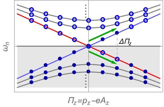
Figure 1: The Landau levels for massless Dirac fermions. Blue and red lines represent the LLL for the right- and left-handed fermions, respectively, and gray curves represent HLLs. Filled (empty) circles represent the occupied (empty) states, and gray shaded region means the Dirac sea. After turning on an electric field adiabatically, right-handed fermions in the LLL obtain the positive energy while left-handed fermions in the LLL develop the holes. The states in the HLLs look unchanged.

3.2 Non-Abelian gauge theory and eta-invariant

We next review the chirality production under external SU(2) gauge field, $A^{a}_{\mu}$, discussed in Ref. Domcke:2018gfr . We consider the following Lagrangian,

$${\cal L}=\mathrm{i}{\bar{\Psi}}\gamma^{\mu}(\partial_{\mu}-\mathrm{i}A_{\mu}^{a}T^{a})\Psi,$$ (19)

where $T^{a}=\sigma^{a}/2$ is the generator of the SU(2) gauge group. The field strength tensor and its dual are given as

$$F_{\mu\nu}^{a} =\partial_{\mu}A_{\nu}^{a}-\partial_{\nu}A_{\mu}^{a}+\epsilon^{0abc}A^{b}_{\mu}A^{c}_{\nu},$$ (20)

$$\tilde{F}^{a\mu\nu} =\frac{1}{2}\epsilon^{\mu\nu\alpha\beta}F_{\alpha\beta}^{a}.$$ (21)

We may define the electric and magnetic fields for the SU(2) field as

$$E_{i}^{a} =F_{i0}^{a},$$ (22)

$$B^{ai} =\frac{1}{2}\epsilon^{0ijk}F_{jk}^{a},$$ (23)

such that the Chern-Pontryagin density is written as

$$F_{\mu\nu}^{a}\tilde{F}^{a\mu\nu}=-4E^{a}_{i}B^{ai}.$$ (24)

One could find the exactly same physics for chirality production as the case of U(1) gauge theory supposing a background field configuration, $A_{\mu}^{a}=\bar{A}_{\mu}n^{a}$ with $\bar{A}_{\mu}=(0,0,-Bx,Et)$. Here $n^{a}$ is an arbitrary constant unit vector. which projects the SU(2) gauge group onto its U(1) subgroup. Once we have in mind the gauge field amplification during axion inflation through the Chern-Simons coupling, $(\phi/4\Lambda)\mathrm{Tr}F_{\mu\nu}^{a}\tilde{F}^{a\mu\nu}$ ($\phi$ is the inflaton and $\Lambda$ is the mass scale related to axion decay constant), however, this configuration is turned out to be unstable for large $(\partial\phi/\partial t)/\Lambda$ due to the non-linear term in $F_{\mu\nu}^{a}$ Domcke:2018rvv . Instead, it has been found that there is a homogeneous and isotropic attractor solution in the presence of the homogeneous axion dynamics as

$$A_{0}^{a}=0,\quad A_{i}^{a}=-f(t)\delta_{i}^{a},$$ (25)

where $f(t)$ is determined by the homogeneous axion velocity $(\partial\phi/\partial t)$. Such a field configuration has been extensively studied in the context of the chromo-natural inflation Adshead:2012kp (see also Ref. Maleknejad:2012wqk ). The electric and magnetic field, as well as the Chern-Pontryagin density for this field configuration is given as

$$E^{a}_{i} ={\dot{f}}\delta^{a}_{i}$$ (26)

$$B^{ai} =f^{2}\delta^{ai}$$ (27)

$$F_{\mu\nu}^{a}\tilde{F}^{a\mu\nu} =-4E^{a}_{i}B^{ai}=-12\dot{f}f^{2}=-4{(f^{3})}^{\cdot}.$$ (28)

Let us stress that here a non-vanishing magnetic field is provided by the homogeneous vector potential, which is distinct from the Abelian case. In the following, we consider the field configuration given by Eq. (25) and investigate the particle production from this background, changing $f$ adiabatically.

One can explicitly solve the Dirac equation in the momentum space under this SU(2) field configuration (25) with $f$ being constant:

$$\left[\mathrm{i}\partial_{t}\pm({\bm{\sigma}}\cdot{\bm{p}}+f{\bm{\sigma}}\cdot{\bm{T}})\right]\psi_{\rm L/R}(t,{\bm{p}})=0,$$ (29)

where $+(-)$ refers left- (right-)handed fermions, respectively, and the SU(2) generators $T^{a}$ acts on the gauge indices of the Dirac field while the Pauli matrices ${\sigma}^{i}$ acts on its spin indices. Without loss of generality, one can take the momentum along the z-direction, ${\bm{p}}=p\hat{e}_{z}$, and introduce the following eigenbases of the spin and gauge degrees of freedom $\chi_{\bm{p}}^{\pm}$ and $t_{\bm{p}}^{\pm}$ satisfying

$$\left(\hat{\bm{p}}\cdot{\bm{\sigma}}\right)\chi_{\bm{p}}^{\pm}=\pm\chi_{\bm{p}}^{\pm},\quad\left(\hat{\bm{p}}\cdot{\bm{T}}\right)t_{\bm{p}}^{\pm}=\pm\frac{1}{2}t_{\bm{p}}^{\pm},$$ (30)

$$\sigma_{\pm}\chi_{\bm{p}}^{\pm}=0,\quad\sigma_{\mp}\chi_{\bm{p}}^{\pm}=2\chi_{\bm{p}}^{\mp},\quad T_{\pm}t_{\bm{p}}^{\pm}=0,\quad T_{\mp}t_{\bm{p}}^{\pm}=t_{\bm{p}}^{\mp},$$ (31)

where $\sigma_{\pm}\equiv\sigma_{1}\pm\mathrm{i}\sigma_{2}$ and $T_{\pm}\equiv T_{1}\pm\mathrm{i}T_{2}$ are ladder operators. Then, the Dirac field can be expanded with these bases

$$\psi_{L/R}(t,{\bm{p}})=\sum_{s,m=\pm}\psi^{(s,m)}_{L/R}(t,{\bm{p}})\chi_{\bm{p}}^{s}t_{\bm{p}}^{m},$$ (32)

and noting that ${\bm{\sigma}}\cdot{\bm{T}}=(\sigma_{+}T_{-}+\sigma_{-}T_{+})/2+\left(\hat{\bm{p}}\cdot{\bm{\sigma}}\right)\left(\hat{\bm{p}}\cdot{\bm{T}}\right)$ the Dirac equation finally becomes

$$\left[\mathrm{i}\partial_{t}\pm\left(p+\frac{f}{2}\right)\right]\psi^{(+,+)}_{\rm L/R}(t,{\bm{p}})=0,$$ (33)

$$\left[\mathrm{i}\partial_{t}\pm\left(-p+\frac{f}{2}\right)\right]\psi^{(-,-)}_{\rm L/R}(t,{\bm{p}})=0,$$ (34)

$$\left[\mathrm{i}\partial_{t}\pm\left(p\left(\begin{array}[]{cc}1&0\\ 0&-1\\ \end{array}\right)+\frac{f}{2}\left(\begin{array}[]{cc}-1&2\\ 2&-1\\ \end{array}\right)\right)\right]\left(\begin{array}[]{c}\psi^{(+,-)}_{\rm L/R}(t,{\bm{p}})\\ \psi^{(-,+)}_{\rm L/R}(t,{\bm{p}})\end{array}\right)=0,$$ (41)

where, once more, $+(-)$ refers left- (right-)handed fermions, respectively. Since $(+,-)$ and $(-,+)$ modes are mixed, one needs to perform diagonalization to identify the energy eigenstates. After diagonalization, one finds the expression of energy dispersion relation for four independent modes as

$$\omega^{(+1)}_{\rm L/R} =\pm\left(-p-\frac{f}{2}\right),$$ (42)

$$\omega^{(-1)}_{\rm L/R} =\pm\left(p-\frac{f}{2}\right),$$

$$\omega^{(0;1)}_{\rm L/R} =\pm\left(-\sqrt{p^{2}+f^{2}}+\frac{f}{2}\right),$$

$$\omega^{(0;2)}_{\rm L/R} =\pm\left(\sqrt{p^{2}+f^{2}}+\frac{f}{2}\right),$$

where $+(-)$ refers left- (right-)handed fermions, respectively. Among these four modes, three modes are gapped and only $\omega^{(-1)}_{\rm L/R}$ smoothly connects the positive frequency state and negative frequency state at $p=f/2$.

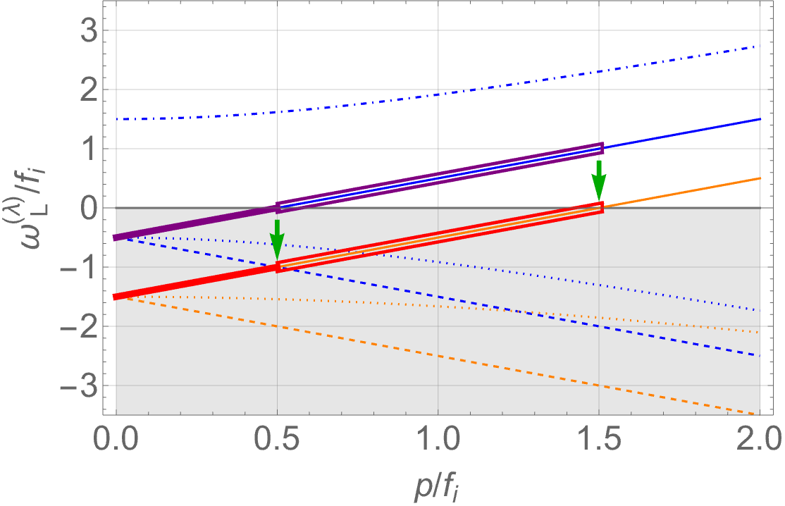
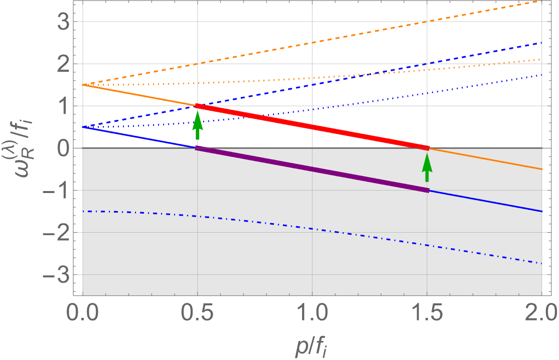
Figure 2: The levels for the massless left- (left figure) and right-handed (right figure) fermions in the background field configuration of SU(2) gauge field (25), respectively. Blue lines are those for $f=f_{i}$ while orange lines are those for $f=f_{f}=3f_{f}$. Solid, dashed, dotted, and dot-dashed lines represent $\omega^{(-1)}_{\rm L/R},\omega^{(+1)}_{\rm L/R},\omega^{(0;1)}_{\rm L/R}$, and $\omega^{(0;2)}_{\rm L/R}$, respectively. Gray shaded region represents the Dirac sea. While for the right-handed fermions states of $\omega=\omega^{(-1)}_{\rm R}$ from $p=f_{i}/2$ to $p=f_{f}/2$ in the Dirac sea at $f=f_{i}$ (red thick line) are excited at $f=f_{f}$ (purple thick line), for the left-handed fermions unoccupied states of $\omega=\omega^{(-1)}$ from $p=f_{i}/2$ to $p=f_{f}/2$ at $f=f_{i}$ (red double line) become holes at $f=f_{f}$ (purple double line). Note that the horizontal axes are those for the physical momenta but not the conjugate momenta, and hence we do not see the sideways shift of the momentum seen in the U(1) case.

By adiabatically evolving $f$ from $f_{i}$ (at $t=t_{i}$) to $f_{f}$ (at $t=t_{f}$) , level crossing occurs for these lowest modes as in the Abelian case where an electric field is applied to LLL. Figure 2 shows the schematic picture of the level crossing in this system. With the normally ordered charge operator, the chiral charge associated with this excitation can be evaluated as

$$\Delta Q_{5}^{(\mathrm{e})}=\Delta Q_{\rm R}^{(\mathrm{e})}-\Delta Q_{\rm L}^{(\mathrm{e})}=\frac{1}{3}\times V\frac{1}{8\pi^{2}}\left(f_{f}^{3}-f_{i}^{3}\right),$$ (43)

where $V\equiv\int\mathrm{d}^{3}x$ is the volume factor, and we have taken into account that in the momentum space there is one state occupied in each volume $V\mathrm{d}^{3}p/(2\pi)^{3}=1$. Since we take the infinite volume limit, we do not discretize the momentum space. In contrast to U(1) case, however, this contribution from excitation does not account for all the fermion chirality:

$$\Delta\langle Q_{5}\rangle=\Delta(\langle Q_{\rm R}\rangle-\langle Q_{\rm L}\rangle)=V\frac{1}{4\pi^{2}}\left(f_{f}^{3}-f_{i}^{3}\right),$$ (44)

which is derived by integrating anomaly equation,

$$\partial_{\mu}J^{\mu}_{5}=-\frac{1}{16\pi^{2}}F_{\mu\nu}^{a}\tilde{F}^{a\mu\nu}=\frac{1}{4\pi^{2}}(f^{3})^{\cdot},$$ (45)

from $t_{i}$ to $t_{f}$ and over whole space. This is because one needs to take into account the vacuum contribution of chiral charge, known as the eta invariant in the Atiyah-Patodi-Singer index theorem Atiyah:1963zz ; Atiyah:1968mp . The theorem indicates the following relation of the charges in our Lorentzian manifold Gibbons:1979kq ; Stone:2023qln :

$$\Delta\langle Q_{5}\rangle=\int\mathrm{d}t\mathrm{d}^{3}x\partial_{\mu}J^{\mu}_{5} =\Delta Q_{\rm R}^{(\mathrm{e})}-\Delta Q_{\rm L}^{(\mathrm{e})}-[\eta_{H}]^{t=t_{f}}_{t=t_{i}},$$ (46)

$$=\Delta Q_{\rm R}^{(\mathrm{e})}-\Delta Q_{\rm L}^{(\mathrm{e})}+\Delta Q_{\rm R}^{(\mathrm{v})}-\Delta Q_{\rm L}^{(\mathrm{v})},$$ (47)

where the vacuum charge can be identified as $\Delta Q_{\rm R/L}^{(\mathrm{v})}=\mp(1/2)[\eta_{H}]^{t=t_{f}}_{t=t_{i}}$. Here $\eta_{H}$ is the eta invariant defined with respect to the Hamiltonian of (right-handed) Weyl fermion as

$$\eta_{H}=\lim_{s\rightarrow 0}\eta_{H}(s),\quad\eta_{H}(s)\equiv\sum_{\omega_{\rm R}\not=0}\mathrm{sgn}(\omega_{\rm R})|\omega_{\rm R}|^{-s}=-\sum_{\omega_{\rm L}\not=0}\mathrm{sgn}(\omega_{\rm L})|\omega_{\rm L}|^{-s},$$ (48)

which diverges and requires an appropriate regularization. In Ref. Domcke:2018gfr , it is shown that the chiral anomaly equation is reproduced with the regularized vacuum contribution

$$\Delta Q_{\rm R/L}^{(\mathrm{v})}=\left[\lim_{\Lambda\rightarrow\infty}-\frac{1}{2}\sum_{\omega_{\rm R/L}\not=0}{\rm sgn}(\omega_{\rm R/L})R\left(\frac{\omega_{\rm R/L}}{\Lambda}\right)\right]^{t=t_{f}}_{t=t_{i}}$$ (49)

where the regulator $R(s)$ is smooth and approaches rapidly to zero sufficiently, and satisfies $R(s\to 0)=1$. By substituting the dispersion (42), chiral charge associated with vacuum contribution is evaluated as

$$\Delta Q_{5}^{(\mathrm{v})} =\Delta Q_{\rm R}^{(\mathrm{v})}-\Delta Q_{\rm L}^{(\mathrm{v})}$$ (50)

$$=[\eta_{H}]^{t=t_{f}}_{t=t_{i}}=\frac{5}{6}\times V\frac{1}{4\pi^{2}}\left(f_{f}^{3}-f_{i}^{3}\right),$$ (51)

with which the net chirality $\Delta\langle Q_{5}\rangle=\Delta Q_{5}^{(\mathrm{e})}+\Delta Q_{5}^{(\mathrm{v})}$ becomes consistent with the prediction of anomaly equation. Let us stress that in contrast to the case of U(1) gauge field, the contribution from gapped modes $\omega^{(+1)}_{\rm L/R},\omega^{(0;1)}_{\rm L/R}$, and $\omega^{(0;2)}_{\rm L/R}$ participates in $\Delta\langle Q_{5}\rangle$ via $\Delta Q_{5}^{(\mathrm{v})}$.

Physically, the eta invariant accounts for the chiral asymmetry accumulated in the vacuum due to the asymmetric energy spectrum of fermions. It is quite interesting that a substantial fraction of the chiral charge lies in the vacuum in this SU(2) gauge field configuration. At this point, one may wonder whether the charge accumulated in the vacuum plays a physical role or not. In other words, it is not clear how this charge interacts with other fields or particles, if ever. For example, there also exists a vacuum contribution in the SU(2) current (not the chiral current) of the fermion in this system. The authors of Ref. Domcke:2018gfr has shown that such a contribution can be renormalized with the running coupling constant and does not interact with other fields. As a result, the backreaction from the fermion to the SU(2) gauge fields is turned out to be inefficient in contrast to the case of U(1) gauge field. Anyway, the above observation indicates that if one needs to distinguish the excitation and vacuum contribution, one should not naively use the integrated anomaly equation (44). This distinction could be more important for the gravitational anomaly and leptogenesis through that as we will see.

3.3 Lessons from gauge field cases

Before proceeding, we summarize what we learn from the chirality production from the point of view of the (Landau) level crossings in the cases of the U(1) and SU(2) gauge fields. For both cases, degeneracy in the helicity and the spin states are broken by the presence of homogeneous magnetic field (or constant $f$ with the non-trivial configuration in the SU(2) case). Consequently, the “lowest” mode globally appears, where the spin polarization is along with the magnetic component of the gauge field, smoothly connecting the negative and positive frequency modes. The generation of chirality is, however, qualitatively different. For the U(1) case, only this lowest mode participates in the chirality generation. That is, the electric field causes momentum shift in LLL and the excited states account for all the chirality generated in this system. On the contrary, the (higher) gapped modes also contribute in the homogeneous and isotropic SU(2) case as the vacuum contribution although level-crossings never take place there. In this case, the amplitude of the SU(2) field value $f$ plays a similar role as the chiral chemical potential and causes chirality dependent bias for all the modes. This is the most striking difference from the U(1) example. Consequently, the evolution of bias $f$ (or the existence of “electric component” of SU(2) field) results in the accumulation of vacuum chiral charge, including the modes without level-crossing.

Although it is sub-leading, the excited states still have non-negligible contribution for SU(2) case. In this respect, we conjecture that for having non-negligible contribution from excitation, homogeneity of the external field seems to play a key role. Because of the homogeneity, the modes relevant for the chiral particle production are globally defined over the whole momentum space, both for the U(1) and SU(2). This global nature allows fermions to have continuous excitation as long as the electric field or growth of $f$ is provided. As we will see in the following, this seems the crucial difference from the chiral spin-2 gravitational field we consider in Sec. 5. As a supporting example of this discussion, let us refer to Ref. Christ:1979zm where the author evaluated the fermion chirality production under the gauge field “radiations” carrying topological charge. Interestingly, for the U(1) case, the vacuum charge accounts for all the chirality generated in this system. Moreover, the U(1) chiral anomaly is recently investigated under the inhomogeneous electric field, which also shows that chiral charge is not produced Fukushima:2023obj .

Another thing we would like to mention here is that, as discussed in Ref. Domcke:2018gfr , there are two conditions for vacuum contribution to be non-vanishing. I) The initial and final external field configuration must not be equivalent up to gauge transformation. II) By definition, the spectrum of positive and negative frequency modes must be asymmetric. Note that both of them are not satisfied in the homogeneous U(1) electromagnetic field case. In order to satisfy the first condition, evolution in the magnetic component of the field is indispensable. If the excitation does not reproduce the anomaly equation and these conditions are satisfied, we can presume that the vacuum contribution would compensate to reproduce the anomaly equation, without a concrete calculation.

As we will see below, the first condition for the existence of the vacuum contribution is always satisfied in the chiral GW generation. In this situation, one may naturally come up with the following question: Can the vacuum contribution be also dominant in gravitational leptogenesis? In fact, the dominance of vacuum asymmetry is observed in the gravitational system, for example, Bianchi type-IX spacetime Gibbons:1979kq ; Gibbons:1979ks and Bianchi type-II spacetime Stone:2023qln . In the following section, before focusing on the system of our interest, flat FLRW plus chiral GWs, we discuss the fermion chirality production in the Bianchi type-IX spacetime. Since it can be decomposed into the closed FLRW spacetime and the standing chiral GWs, the investigation of this system may provide us a hint to understand the physics of gravitational leptogenesis.

4 A solvable exmaple in gravitational system: Bianchi type-IX spacetime

Now let us turn to the chirality production under the non-trivial gravitational background. Before examining the configuration motivated from the gravitational leptogenesis, we first review the case with closed homogeneous spacetime, classified according to the Bianchi type models.

Among the Bianchi classification of the homogeneous $3+1$ spacetime, Bianchi type-IX is particularly of our interest. As discussed in Refs. Grishchuk:1974ny ; King:1991jd , this spacetime can be expressed as a closed FLRW spacetime onto which circularly polarized GWs are superimposed. This fact motivates us to investigate the gravitational chiral anomaly in this system since the circular polarization of GWs yields non-vanishing Chern-Pontryagin density. Indeed, Gibbons has discussed gravitational production of neutrino in the evolving spacetime which starts from ”polarized” initial state to the isotropic (unpolarized) final state Gibbons:1979ks ; Gibbons:1979kq . Let us give a review on how the chirality of fermion is generated in this system with certain clarification compared to the previous studies.

4.1 Bianchi type-IX and GW interpretation

We first briefly review the general characteristics of Bianchi type-IX spacetime, following the discussion in Ref. King:1991jd . A right-homogeneous Bianchi type-IX spacetime is generally described by a metric (with the Cartan calculus) as

$$\mathrm{d}s^{2} =-a^{2}(\eta)(\mathrm{d}\eta^{2}-\mathrm{d}l^{2}),$$ (52)

$$\mathrm{d}l^{2} =A_{ij}(\eta)\lambda^{i}\otimes\lambda^{j},$$ (53)

where $\eta$ is the conformal time, and $\left\{\lambda^{i}\right\}$ are three left-invariant 1-form on the 3-sphere $S^{3}$ satisfying

$$\mathrm{d}\lambda^{i}=\frac{1}{S}\epsilon_{ijk}\lambda^{j}\wedge\lambda^{k}.$$ (54)

More concretely, they can be expressed as

$$\lambda^{1} =\frac{S}{2}\left[-\sin\psi\mathrm{d}\theta+\sin\theta\cos\psi\mathrm{d}\phi\right],$$ (55)

$$\lambda^{2} =\frac{S}{2}\left[\cos\psi\mathrm{d}\theta+\sin\theta\sin\psi\mathrm{d}\phi\right],$$ (56)

$$\lambda^{3} =\frac{S}{2}\left[\cos\theta\mathrm{d}\phi+\mathrm{d}\psi\right],$$ (57)

with $(\theta,\psi,\phi)$ being the Euler angles which run $0\leq\theta\leq\pi,\ 0\leq\psi\leq 2\pi,\ 0\leq\phi\leq 4\pi$ Misner:1969hg , and $S$ being the (comoving) radius of $S^{3}$. The spatial part of the metric (53) can be decomposed into the background closed sphere (or the closed FLRW Universe) and the five independent tensor fields as

$$A_{ij}(\eta)=A_{0}(\eta)\delta_{ij}+\sum_{a=1}^{5}A_{a}(\eta)C^{a}_{ij},$$ (58)

where $C^{a}_{ij}$ are five linearly independent traceless matrices. While the isotropy of background sphere is broken, the tensor fields $A_{a}(\eta)C^{a}_{ij}\lambda^{i}\otimes\lambda^{j}$ imposed onto the sphere preserves its right homogeneity. In this sense, one can understand that the Bianchi type-IX spacetime is an anisotropic generalization of the closed FLRW Universe.

Another aspect of this spacetime we would like to mention is that this anisotropy of closed sphere involves the parity-violation. As shown in Ref. King:1991jd , the right homogeneous tensor fields described by $A_{a}(\eta)C^{a}_{ij}\lambda^{i}\otimes\lambda^{j}$ are the symmetric, transverse, and traceless tensor spherical harmonics on the background 3-sphere. In other words, they can be understood as the standing GWs around the sphere with the longest wavelength. In addition, these waves have the left-circular polarization (see Ref. King:1991jd for graphical description). Therefore, the right homogeneous Bianchi type-IX spacetime can be decomposed into the background closed sphere plus left circularly polarized GWs Grishchuk:1974ny ; King:1991jd . Note that the same discussion applies to the left homogeneous Bianchi type-IX and in this case the spacetime is wrapped by the right circularly polarized GWs. As we will see below with a specific example of the metric, parity-violating GWs yield non-vanishing Chern-Pontryagin density. Therefore, this spacetime can be a playground to investigate the generation of fermion chirality.

Now we consider a specific class of this spacetime called as the axial Bianchi type-IX, which was considered in Refs. Gibbons:1979kq ; Gibbons:1979ks to examine the chiral fermion production. The metric of the axial Bianchi type-IX is given as

$$\mathrm{d}s^{2} =-a(\eta)^{2}\left(\mathrm{d}\eta^{2}-(e^{2\beta_{+}(\eta)}\lambda^{1}\otimes\lambda^{1}+e^{2\beta_{+}(\eta)}\lambda^{2}\otimes\lambda^{2}+e^{-4\beta_{+}(\eta)}\lambda^{3}\otimes\lambda^{3})\right),$$

$$=-a(\eta)^{2}\left(\mathrm{d}\eta^{2}-\frac{S^{2}}{4}\left[e^{2\beta_{+}(\eta)}\mathrm{d}\theta^{2}+\left(e^{2\beta_{+}(\eta)}\sin^{2}\theta+e^{-4\beta_{+}(\eta)}\cos^{2}\theta\right)\mathrm{d}\phi^{2}\right.\right.$$

$$\left.\left.\ \ \ \ \ +2e^{-4\beta_{+}(\eta)}\cos\theta\mathrm{d}\phi\mathrm{d}\psi+e^{-4\beta_{+}(\eta)}\mathrm{d}\psi^{2}\right]\right),$$ (59)

where $\beta_{+}$ is a function of time and characterizes the anisotropy of the closed sphere. At the same time, $\beta_{+}$ also characterizes the amplitude of the polarized GWs. This can be seen by performing the decomposition mentioned above:

$$\mathrm{d}s^{2}=-a(\eta)^{2}\left(\mathrm{d}\eta^{2}-\left(\mathrm{d}l^{2}_{B}+\mathrm{d}l^{2}_{h}\right)\right),$$ (60)

where $\mathrm{d}l^{2}_{B}$ is the background sphere,

$$\mathrm{d}l^{2}_{B} =\frac{(2e^{2\beta_{+}}+e^{-4\beta_{+}})}{3}\delta_{ij}\lambda^{i}\otimes\lambda^{j}$$

$$=\frac{(2e^{2\beta_{+}}+e^{-4\beta_{+}})}{3}\frac{S^{2}}{4}\left[\mathrm{d}\theta^{2}+\mathrm{d}\phi^{2}+2\cos\theta\mathrm{d}\phi\mathrm{d}\psi+\mathrm{d}\psi^{2}\right].$$ (61)

On the other hand, $\mathrm{d}l^{2}_{h}$ is the standing GW described by one specific mode ($a=5$ in Eq. (58) if we follow the notation in Ref. King:1991jd )

$$\frac{1}{\sqrt{6}}\left(-\lambda^{1}\otimes\lambda^{1}-\lambda^{2}\otimes\lambda^{2}+2\lambda^{3}\otimes\lambda^{3}\right)$$ (62)

as

$$\mathrm{d}l^{2}_{h} =\frac{(e^{2\beta_{+}}-e^{-4\beta_{+}})}{3}\left(\lambda^{1}\otimes\lambda^{1}+\lambda^{2}\otimes\lambda^{2}-2\lambda^{3}\otimes\lambda^{3}\right)$$

$$=\frac{(e^{2\beta_{+}}-e^{-4\beta_{+}})}{3}\frac{S^{2}}{4}\left[\mathrm{d}\theta^{2}+(1-3\cos^{2}\theta)\mathrm{d}\phi^{2}-4\cos\theta\mathrm{d}\phi\mathrm{d}\psi-2\mathrm{d}\psi^{2}\right].$$ (63)

Note that the standing GW is not restricted to be perturbative as ordinary GWs. Hence, this expression in the large anisotropy limit $\beta_{+}\gg 1$ still makes sense.

For this metric (59), the gravitational Chern-Pontryagin density $R\tilde{R}$ is evaluated as

$$R\tilde{R} =-\frac{48}{a^{4}S^{3}}\beta_{+}^{\prime}\left(4k^{4}-4k^{2}-6S^{2}k^{4/3}\beta_{+}^{\prime 2}+3S^{2}k^{4/3}\beta_{+}^{\prime\prime}\right)$$

$$=\frac{1}{\sqrt{-g}}\partial_{\eta}\left(6\sin\theta\left(\frac{1}{3}(k^{2}-1)^{2}-\frac{3S^{2}}{2}k^{4/3}\beta_{+}^{\prime 2}\right)\right),\quad\text{with}\quad k\equiv\exp(-3\beta_{+}),$$ (64)

where $g=-S^{6}a^{8}\sin^{2}\theta/64$ is the determinant of the metric and the prime denotes the derivative with respect to the conformal time. Here we have introduced a new parameter $k$ following Refs. Gibbons:1979kq ; Gibbons:1979ks . One can see that $R\tilde{R}$ becomes non-vanishing when the anisotropy $\beta_{+}$ (or $k$) evolves. This is a clear indication of parity-violation due to the polarized GW, which may be quantified by the gravitational helicity density defined as

$$\sqrt{-g}K^{0}=6\sin\theta\left(\frac{1}{3}(k^{2}-1)^{2}-\frac{3S^{2}}{2}k^{4/3}\beta_{+}^{\prime 2}\right).$$ (65)

Since the spacetime with different $\beta_{+}$ or $k$ is not equivalent up to the gauge transformation, the first condition for the existence of the vacuum contribution in the particle production is satisfied. This motivates us to investigate the particle production in terms of the level crossing to clarify the distribution of chiral charge.

4.2 Chirality production and comparison to the SU(2) gauge example

We now see the chirality production in the point of view of the level crossing. According to the gravitational chiral anomaly equation,

$$\nabla_{\mu}J^{\mu}_{5}=\frac{1}{\sqrt{-g}}\partial_{\mu}(\sqrt{-g}J^{\mu}_{5})=-\frac{1}{12(4\pi)^{2}}R\tilde{R},$$ (66)

we would expect that the fermion chirality production takes place when $\beta_{+}$ (or $k$) changes. Integration of the chiral anomaly equation (64) leads to

$$\Delta Q_{5} =-\int_{0}^{\pi}\mathrm{d}\theta\int_{0}^{2\pi}\mathrm{d}\psi\int_{0}^{4\pi}\mathrm{d}\phi\frac{\sin\theta}{2(4\pi)^{2}}\Delta\left(\frac{1}{3}(k^{2}-1)^{2}-\frac{3S^{2}}{2}k^{4/3}\beta_{+}^{\prime 2}\right)$$

$$=-\frac{1}{6}\Delta\left((k^{2}-1)^{2}-3k^{4/3}(\beta^{\prime}[\eta])^{2}\right).$$ (67)

Then we wonder how they are divided into the excitation and vacuum contribution. Following Refs. Gibbons:1979kq ; Gibbons:1979ks , let us discuss the generation of fermion chirality under the adiabatic evolution of the spacetime assuming $\beta_{+}^{\prime}\to 0$.

Since the Bianchi-IX space has an SU(2) structure as seen in Eq. (54), it is convenient to study the system in the frame with the Cartan calculus (see Eq. (53)). The Dirac equation for the massless fermion in that frame is given as Brill:1966tia

$$\mathrm{i}\gamma^{\mu}(\omega_{\mu}(\Psi)-\Gamma_{\mu}\Psi)=0,$$ (68)

where $\omega_{\mu}$ are the dual of the normalized 1-forms in 4 dimension $\omega^{\mu}$, such that it forms Minkowskian metric. The connection $\Gamma_{\mu}$ is defined as

$$\Gamma_{\mu}=-\frac{1}{4}\omega_{\mu\nu\rho}\gamma^{\nu}\gamma^{\rho},$$ (69)

where $\omega^{\mu}_{\ \ \nu\rho}$ satisfies $d\omega^{\mu}=\omega^{\mu}_{\ \ \nu\rho}\omega^{\nu}\wedge\omega^{\rho}$.

In our case of Eq. (59), the Dirac equation can then be expressed as

$$(\mathrm{i}\partial_{\eta}\mp D)(a^{3/2}(\eta)\psi_{L/R})=0,$$ (70)

where - (+) refers left- and right-handed fermions, respectively, and the Dirac operator $D$ is defined as

$$D =\frac{k^{1/3}}{S}\left(\begin{array}[]{cc}\dfrac{2L_{(3)}}{k}+\left(\dfrac{1}{k}+\dfrac{k}{2}\right)&2L_{-}\\ 2L_{+}&-\dfrac{2L_{(3)}}{k}+\left(\dfrac{1}{k}+\dfrac{k}{2}\right)\end{array}\right).$$ (73)

Here we have have dropped the terms proportional to $\beta_{+}^{\prime}$ and defined

$$L_{(i)}\equiv-\frac{\mathrm{i}S}{2}\xi_{(i)},\quad L_{\pm}=L_{(1)}\pm\mathrm{i}L_{(2)}.$$ (74)

The constant terms $(1/k+k/2)$ comes from the connection, while terms with $L_{(i)}$ comes from $\omega_{\mu}$. Note that $\{L_{(i)}\}$ satisfy the spin algebra,

$$[L_{(i)},L_{(j)}]=\mathrm{i}\epsilon_{ijk}L_{(k)},\quad[L_{(3)},L_{\pm}]=\pm L_{\pm},$$ (75)

and hence $L_{\pm}$ can be understood as the ladder operators. Then we can introduce eigenfunction $\left|l,m,n\right\rangle$ as

$$L_{3}\left|l,m,n\right\rangle =n\left|l,m,n\right\rangle,$$ (76)

$$L_{\pm}\left|l,m,n\right\rangle =\sqrt{(l\mp n)(l\pm n+1)}\left|l,m,n\pm 1\right\rangle,$$ (77)

where $l$ is a non-negative half-integer or a natural number, and $m,n$ are (half-) integers satisfying $m,n=-l,-l+1,...,l-1,l$. Here the quantum number $m$ is introduced because these states are also representations of the right-translations. Using this function, eigenstates of the Dirac operator (73) can be constructed as

$$\Phi_{\pm}(l,m,n)=\left(\begin{array}[]{c}\left(n/k\pm\sqrt{(n/k)^{2}+(l+1/2)^{2}-n^{2}}\right)|l,m,n-1/2\rangle\\ \sqrt{(l+1/2)^{2}-n^{2}}|l,m,n+1/2\rangle\end{array}\right),$$ (80)

whose eigenvalues are

$$\frac{k^{1/3}}{S}\left(\dfrac{k}{2}\pm 2\sqrt{\left(\dfrac{n}{k}\right)^{2}+\left(l+\dfrac{1}{2}\right)^{2}-n^{2}}\right),$$ (81)

Here $m$ runs from $-l$ to $l$, which gives a degeneracy $2l+1$, while $n$ runs from $-l-1/2$ to $l+1/2$. Note that for $|n|=l+1/2$, we only have $\Phi_{+}(l,m,l+1/2)$ since $\Phi_{-}(l,m,l+1/2)$ is a null state. Thus we obtain the energy dispersion relation as

$$\omega_{L}^{\pm}(l,m,n) =\frac{k^{1/3}}{S}\left(\dfrac{k}{2}\pm 2\sqrt{\left(\dfrac{n}{k}\right)^{2}+\left(l+\dfrac{1}{2}\right)^{2}-n^{2}}\right),$$ (82)

$$\omega_{R}^{\pm}(l,m,n) =-\frac{k^{1/3}}{S}\left(\dfrac{k}{2}\pm 2\sqrt{\left(\dfrac{n}{k}\right)^{2}+\left(l+\dfrac{1}{2}\right)^{2}-n^{2}}\right).$$ (83)

for the left- and right-handed fermions, respectively. While $\omega_{L}^{+}$ and $\omega_{R}^{+}$ are positive and negative definite, respectively, $\omega_{L}^{-}$ and $\omega_{R}^{-}$ connects the positive and negative energy eigenstates. Figure 3 shows the dispersion relation of the left-handed fermions for $n=0$ and some choices of $k$.

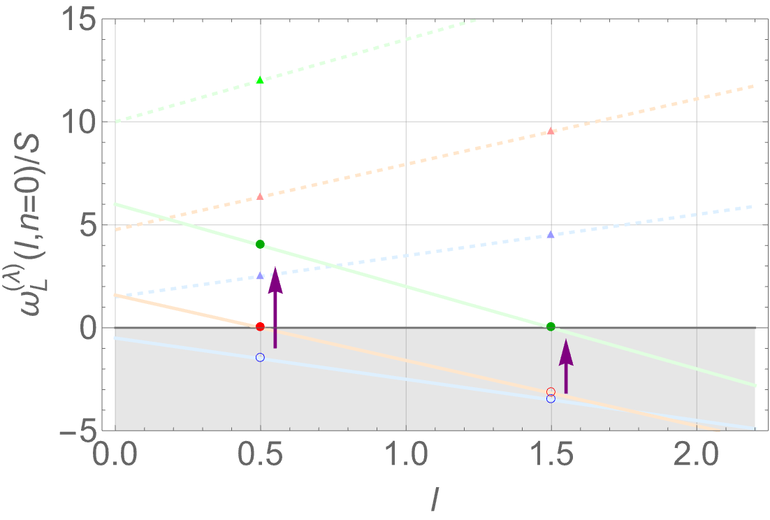
Figure 3: The levels for the massless left-handed fermions in the Bianchi IX spacetime (59) for $n=0$. Blue, red, and green lines and markers are those for $k=1,4,8$, respectively. Solid lines and circles represent $\omega_{L}^{-}$ while dashed lines and triangles represent $\omega_{L}^{+}$. Gray shaded region represents the Dirac sea. While all the states of $\omega_{L}^{-}$ are in the Dirac sea for $k=1$, the highest state $l=1/2$ appears as the excitation at $k=4$ while the state $l=3/2$ appears at $k=8$.

As can be seen from Eqs. (82) and (83), in the isotropic background ($k=1$), all the states of $\omega^{-}_{L}$ are in the Dirac sea and those of $\omega^{-}_{R}$ have positive definite energy eigenvalue. The sign of eigenvalue $\omega^{-}_{L/R}$ can be flipped for large enough $k$, or in other words, “non-perturbatively” large amplitude of the standing wave. For example, the lowest energy state $(l,n)=(1/2,0)$ changes the sign at $k=4$. Therefore, if the universe evolving from the vacuum isotropic space to large $k$, left-handed fermions appear as excitations while right-handed fermions develop holes as a consequence of the zero-crossing, which leads to a negative chirality production (or vice versa as discussed in Refs. Gibbons:1979ks ; Gibbons:1979kq ), This excited contribution of chiral charge is then evaluated as

$$\Delta Q_{5}^{(\mathrm{e})}=\Delta Q_{R}^{(\mathrm{e})}-\Delta Q_{L}^{(\mathrm{e})}=-\sum_{l,n}2(2l+1).$$ (84)

where $(l,n)$ runs the states that experiences the level crossing. Here $2l+1$ counts the degeneracy of $m$ and 2 counts the left- and right-handed fermions.

In the large $k$ limit, we can obtain an approximate evaluation by replacing the summation to the integral, $\int dldn$, with the region of $(l,n)$,

$$|n|\leq l-\frac{1}{2},\quad\left(l+\frac{1}{2}\right)^{2}-n^{2}<\frac{k^{2}}{16},$$ (85)

which leads to

$$\Delta Q_{5}^{(\mathrm{e})}\simeq-\frac{k^{4}}{256}.$$ (86)

The $k$ dependence, $\Delta Q_{5}^{(\mathrm{e})}\propto k^{4}$, is the same to the anomaly equation (67). This means that the level crossing contribution continues to be non-negligible with respect to $\Delta Q_{5}$ even in $k\to\infty$ limit. We anticipate that this feature is due to the homogeneity of system as we discussed in Sec. 3.3. That is, the system admits globally defined momentum (or the infinite sets of label $(l,m,n)$) over phase space and also global selection of spin states. Therefore, as long as the anisotropy increases (or decreases), there will always be modes excited as in the gauge field examples.

There is, however, an order of magnitude difference between $\Delta Q_{5}^{(\mathrm{e})}$ and $\Delta Q_{5}$ predicted from the anomaly equation (67). Moreover at $k<4$ there are no level crossing at all as has been seen in Fig. 3, while the anomaly equation (67) suggests the generation of the chiral asymmetry for any $k>1$. This indicates that the chirality is not mainly carried by the particles (excitation) but the vacuum. Indeed, Ref. Hitchin:1974rbi has shown that for $k<4$ the eta invariant is evaluated (see also Ref. Stone:2023qln ) as

$$\eta_{H}(0)=-\frac{1}{6}(1-k^{2})^{2},$$ (87)

while larger $k$ we shall subtract the (sub-dominant) contribution of the level-crossing. Since the eta invariant in the small anisotropy regime (87) fully agrees with the chiral asymmetry predicted by the anomaly equation (67), we safely conclude that the anomaly equation holds by taking into account both the excitation and vacuum contribution,

$$\Delta Q_{5}=\Delta Q_{5}^{(\mathrm{e})}+\Delta Q_{5}^{(\mathrm{v})},\quad\Delta Q_{5}^{(\mathrm{v})}=[\eta_{H}(0)]_{t=t_{i}}^{t=t_{f}}.$$ (88)

We now obtain further qualitative insights on the chiral anomaly in this system by comparing to the homogeneous SU(2) gauge field case. From Eqs. (82) and (83), one can easily see that the spatial anisotropy $k$ behaves similar to the chemical potential $\mu_{\rm R/L}$ and breaks the degeneracy as it causes energy bias $\sim k^{4/3}/2S$ between the positive and negative energy mode. This is similar to the case with homogeneous SU(2) gauge field discussed in Sec. 3.2, where the energy bias $f/2$ leads to chirality production in a very different way from the Abelian case. It is interesting to note that the bias term in the Dirac operator (73) comes from the connection term in Eq. (68) and can be regarded as the “non-Abelian” contribution of the homogeneous but anisotropic geometry. Note that the bias term exists even for the background sphere without GWs, $\beta_{+}=0$ or $k=1$. Therefore, one might expect that such a chemical potential-like bias could arise if the “non-Abelian” nature is inherent to the spacetime geometry, which is already curved at the background.. Such a concordance reminds us the sub-leading (but non-negligible) contribution from the smooth excitation and the domination of vacuum contribution in the SU(2) case. Then, the distribution of chiraliy in the Bianchi type-IX discussed above is no longer surprising to us.

Let us summarize this section with a comment on the GW interpretation of the Bianchi type-IX spacetime. If one assumes $|\beta_{+}|\ll 1$, the amplitude of gravitational standing waves becomes small enough and they seems to resemble the “ordinary” GWs which are the fluctuation around the “flat” spacetime. As we will discuss below, however, the ordinary GWs are essentially different from the standing GWs around closed sphere. Therefore, while the fact that level-crossing does not occur unless the amplitude of standing wave is non-perturbatively large is suggestive, one cannot simply apply this result to the fluctuation around (conformally) flat spacetime. On the other hand, we have seen a concordance of the chirality generation between the Bianchi type-IX case and the homogeneous SU(2) gauge field case. This suggests that a deeper understanding of the chirality generation under the external gauge field may help us to understand that generated by the parity-violating gravitational field. With this spirit, in the following section we discuss the fermion chirality generation under chiral GWs around flat spacetime based on the analogy between the classical electromagnetism and the weak gravitational fields.

5 Investigation of the Dirac equation under the parity-violating weak spin-2 field

In this section, to obtain the insights on the gravitational leptogenesis, we investigate the effect of weak spin-2 gravitational field around the Minkowski spacetime on the massless Dirac fermion. We first introduce a toy model for the parity-violating spin-2 gravitational background yielding $R\tilde{R}\neq 0$, which is a simple extension of the U(1) gauge field configuration discussed in Sec. 3.1 and would be suitable for examining the gravitational leptogenesis. This system is, however, hard to solve analytically in contrast to the U(1) case. Therefore, in order to understand intuitively, we tackle this system by relying on the analogy between the classical electromagnetism and weak gravity. We find that spin-2 nature of the gravity seems to make the level crossing less efficient than U(1) case.

5.1 Similarity to electromagnetism

5.1.1 Dirac equation under the weak gravitational field

We first investigate the field equation for the massless Dirac fermion in the weak gravitational field background, where we find an “Abelian”-like nature, or that is similar to the helical U(1) gauge fields. Here we consider the metric perturbation around the Minkowski spacetime: $g_{\mu\nu}=\eta_{\mu\nu}+h_{\mu\nu}$. Throughout this section, we impose the TT gauge condition to pick up the spin-2 contribution . The massless Dirac equation in the curved spacetime is given as Birrell:1982ix ; Parker:2009uva

$$\mathrm{i}\gamma^{a}e^{\mu}_{\ a}D_{\mu}\psi=0,\quad D_{\mu}\equiv\partial_{\mu}-\frac{\mathrm{i}}{4}\omega_{\mu ab}\sigma^{ab},$$ (89)

where $e^{\mu}_{\ a}$ is the tetrad that satisfies $g^{\mu\nu}=e^{\mu}_{\ a}e^{\nu}_{\ b}\eta^{ab}$, $\omega_{\mu}^{\ ab}=e_{\nu}^{\ a}\Gamma^{\nu}_{\ \sigma\mu}e^{\sigma b}+e_{\nu}^{\ a}\partial_{\mu}e^{\nu b}$ ($\Gamma^{\nu}_{\ \sigma\mu}$ is the Christoffel symbol) is the spin connection, and $\sigma^{ab}=(\mathrm{i}/2)[\gamma^{a},\gamma^{b}]$. The tetrad and the spin connections around the Minkowski spacetime are expanded in terms of $h_{ij}$ (see Eq. (2)) as

$$e^{i}_{\ a}\simeq\delta^{i}_{\ a}-\frac{1}{2}\eta^{ik}h_{ka}+\mathcal{O}(h^{2}),\quad\omega_{\mu ab}=\frac{1}{2}(\partial_{b}h_{\mu a}-\partial_{a}h_{\mu b}),$$ (90)

such that the Dirac equation can be expanded as

$$\left\{\mathrm{i}\partial_{t}\pm\mathrm{i}\left(\delta^{j}_{\ i}-\frac{1}{2}h^{j}_{\ i}\right)\sigma^{i}\partial_{j}\right\}\psi_{R/L}(t,\bm{x})=0.$$ (91)

Note that from the TT gauge condition we find $\omega_{0ab}=0$ and $\gamma^{i}\omega_{iab}\sigma^{ab}=\gamma^{i}\Gamma_{i}=0$ at the linear order in $h_{ij}$, and hence $h_{ij}$ in Eq. (91) comes solely from the tetrad in Eq.(89). This is quite in contrast to the small GW amplitude limit $\beta_{+}\ll 1$ of Bianchi type-IX case where $\gamma^{i}\Gamma_{i}\neq 0$ at the leading order of $\beta_{+}$ (or $h_{ij}$) and the energy bias still appears (even for $\beta_{+}=0$). This is because the Bianchi type-IX spacetime is the deformation of an already-curved spacetime (more specifically, a closed sphere), where the spin connection yields non-vanishing $\gamma^{i}\Gamma_{i}$. While this bias term is important for the particle production (as well as the emergence of the vacuum contribution) in the Bianchi type-IX case, the gravitational leptogenesis occurs in the system with the parity-violating GWs around the conformally flat spacetime. Therefore, to investigate how the particle production takes place in gravitational leptogenesis, we cannot use the result in the Bianchi type-IX spacetime directly and we need to examine the Dirac equation Eq. (91). Note that in the gravitational leptogenesis introduced in Sec. 2, the lepton asymmetry is generated at the level of linear perturbation.

By using the plane wave ansatz formally,

$$\psi_{R/L}(t,\bm{x})=e^{i\bm{p}\cdot\bm{x}}{\tilde{\psi}}_{R/L}(t,\bm{x};\bm{p}),$$ (92)

where ${\tilde{\psi}}_{R/L}(t,\bm{x};\bm{p})$ does not depend explicitly on $\bm{x}$, the equation of motion becomes

$$\left\{\mathrm{i}\partial_{t}\mp\left(\bm{\sigma}\cdot\bm{p}\right)\pm\frac{1}{2}h_{ij}\sigma_{i}p_{j}\right\}{\tilde{\psi}}_{R/L}(t,\bm{x};\bm{p})=0.$$ (93)

Note that $p_{i}$ is the “momentum” associated with the background flat spacetime $\eta_{\mu\nu}$, but not the quantity defined for the full spacetime $g_{\mu\nu}(=\eta_{\mu\nu}+h_{\mu\nu})$. Indeed, in the case of Bianchi type-IX spacetime preserving homogeneity, we can take the invariant basis on which $h_{ij}$ becomes constant and easily find the momentum globally defined. As usually done in the study of cosmological perturbation theory, we use this flat spacetime momentum and regard the last term as an interaction between the “external field” $h_{ij}$ and the Dirac field. One can formally identify the external $h_{ij}$ field with a U(1) gauge field as

$$A_{j}\equiv(1/2)h_{ij}p_{i},$$ (94)

which the fermion with momentum $p_{i}$ feels. Here $A_{j}$ satisfies the Lorentz gauge condition due to the TT gauge condition and hereafter we shall refer to it as geometric gauge field.

5.1.2 A toy field configuration of parity-violating weak spin-2 field

Next we construct a parity-violating configuration of weak gravitational fields, which would be suitable to investigate the situation of our interest. The construction can be done in a similar fashion to the helical U(1) gauge fields studied in Sec. 3.1, by making an analogy to the classical electromagnetism and weak gravity.

Under the TT gauge condition, we can linearize the Riemann curvature tensor as

$$R^{\tau}_{\ \sigma\mu\nu}\simeq\partial_{\mu}\Gamma^{\tau}_{\nu\sigma}-\partial_{\nu}\Gamma^{\tau}_{\mu\sigma}\simeq\partial_{\mu}\left\{\frac{1}{2}\left(\partial_{\sigma}h_{\nu}^{\ \tau}-\partial^{\tau}h_{\nu\sigma}\right)\right\}-\partial_{\nu}\left\{\frac{1}{2}\left(\partial_{\sigma}h_{\mu}^{\ \tau}-\partial^{\tau}h_{\mu\sigma}\right)\right\}.$$ (95)

With the naive identification of $\Gamma_{\mu\sigma}^{\tau}$ with a gauge field, one can see the similar structure between the linearized Riemann curvature tensor and the field strength of Abelian gauge field (7). This similarity in the structure of electromagnetism and gravity has been widely investigated in the field of “gravito-electromagnetism” (GEM). The interested readers can refer to, for example, Ref. Mashhoon:2003ax as a comprehensive review of GEM.

This correspondence motivates us to define the “electric-like” component and the “magnetic-like” component of the curvature tensor as follows:

$$E_{i\sigma\tau} \equiv R_{i0\sigma\tau}\simeq\frac{1}{2}\left(\partial_{\sigma}\dot{h}_{i\tau}-\partial_{\tau}\dot{h}_{i\sigma}\right),$$ (96)

$$B^{i}_{\ \sigma\tau} \equiv\frac{1}{2}\frac{\epsilon^{0ijk}}{\sqrt{-g}}R_{jk\sigma\tau}\simeq\frac{1}{2}\epsilon^{ijk}\partial_{j}\left(\partial_{\tau}h_{k\sigma}-\partial_{\sigma}h_{k\tau}\right).$$ (97)

With these components, we can express the Chern-Pontryagin density as

$$R\tilde{R}=-4E_{i\sigma\tau}B^{i\sigma\tau},$$ (98)

which is a similar expression with the decomposition of $F\tilde{F}$ in Eq. (11). Under the TT gauge condition, $E_{ij0}$ and $E_{ijk}$, $B_{ij0}$ and $B_{ijk}$ generically become non-vanishing.

It is known that for GWs, $R\tilde{R}$ quantifies the asymmetry between the left and right circular polarizations. Particularly, it measures the growth in deviation from the on-shell solution for each polarization as $\partial_{t}\left(|\dot{h}_{\rm R/L}(t)|^{2}-k^{2}|h_{\rm R/L}(t)|^{2}\right)+\mathcal{O}(h^{4})$, where $h_{\rm R/L}(t)$ abstractly represents the amplitude of the mode with wave number $k$. This means that when $|\dot{h}_{\rm R/L}(t)|^{2}$ has non-trivial evolution in the left-right asymmetric manner, $R\tilde{R}$ becomes non-vanishing. One can easily check that $\partial_{t}|\dot{h}_{\rm R/L}(t)|^{2}$ contribution arises from $E_{ij0}B^{ij0}$ in $R\tilde{R}$. Indeed, in the gravitational leptogenesis, the lepton asymmetry is evaluated by picking up from this lowest order contribution of $h_{\rm R/L}(t)$ in $R\tilde{R}$. Therefore, hereafter we shall investigate the configuration of $h_{ij}$ in the linear perturbation with which both of $E_{ij0}$ and $B_{ij0}$ are non-vanishing.

In a similar way to the helical U(1) gauge field studied in Sec. 3.1, we can construct a parity-violating gravitational field configuration where both of $E_{ij0}$ and $B_{ij0}$ are non-vanishing as follows. In terms of $h_{ij}$, $E_{ij0}$ and $B_{ij0}$ are expressed as

$$E_{ij0} =-\frac{1}{2}\ddot{h}_{ij},$$ (99)

$$B^{i}_{\ j0} =\frac{1}{2}\epsilon^{ilm}\partial_{l}\dot{h}_{mj}.$$ (100)

From these expressions, one can see that formally, $\mathcal{A}_{ij}\equiv(1/2)\dot{h}_{ij}$ is quite similar to the vector potential $A_{\mu}$. In the gravitational leptogenesis, GWs distribute as stochastic variables with a certain coherence length, in a similar way to the electric and magnetic fields in the U(1) case studied in Ref. Domcke:2018eki . Following the approach there, it would be appropriate to study the system with a constant electric and magnetic-like component of the curvature tensors, $E_{ij0}$ and $B_{ij0}$. By comparing to the configuration $A_{\mu}=(0,0,By,Et)$ resulting in a constant $F\tilde{F}=4EB$ (see Eq. (12)), we find that

$$\mathcal{A}_{ij}=\left(\begin{array}[]{ccc}Et&-Bz&0\\ -Bz&-Et&0\\ 0&0&0\end{array}\right),$$ (101)

where we shall restrict ourselves to small intervals of $t$ and $z$ for perturbativity. The configuration (101) resembles GW running in the $z$ direction and gives a constant and parallel $E$ and $B$ tensor in $x$-$y$ direction as $B_{110}=-B_{220}=B$ and $E_{110}=-E_{220}=-E$ at the first order in the perturbation. This leads to $R\tilde{R}=16EB$, which could be the counterpart of the homogeneous and aligned electromagnetic field, and we expect that the chirality should be generated according to the anomaly equation. Note that $E_{ijk}$ has non-vanishing component such as $E_{123}=B$ in the present case but it should not contribute to the chiral anomaly since $B^{ijk}=0$. In the next subsection, we discuss how this geometric U(1) gauge field with the metric (101) affects the fermion field through the Dirac equation (93).

5.2 Application of U(1) gauge physics to the weak spin-2 gravitational field

Now we try to examine the dynamics of fermions on the spacetime with the metric (101). The explicit form of the geometric gauge field (94) for a fermion with momentum $p_{i}$ can be given as

$$A_{x}=\frac{1}{2}Et^{2}p_{x}-Btzp_{y},\ \ \ A_{y}=-\frac{1}{2}Et^{2}p_{y}-Btzp_{x},\ \ \ A_{z}=0.$$ (102)

Note that the spacetime dependence of $A_{x/y}$ is the second order to yield non-vanishing $R\tilde{R}$, which has one additional derivative compared to $F\tilde{F}$. This is originated from the difference in the order of derivatives between the Riemann tensor and gauge field strength tensor. Eq. (94) results in the following geometric “electric and magnetic fields”, $E_{i}\equiv-\partial_{t}A_{i}$, $B^{i}=\epsilon^{ijk}\partial_{j}A_{k}$, as

$$E_{x} =-Etp_{x}+Bzp_{y},\ \ \ E_{y}=Etp_{y}+Bzp_{x},\ \ \ E_{z}=0,$$ (103)

$$B_{x} =Btp_{x},\ \ \ B_{y}=-Btp_{y}\ \ \ B_{z}=0.$$

From the Dirac equation (90) with the identification (94), a fermion particle with momentum $p_{i}$ would feel the electric force as ${\bm{F}}={\bm{E}}=(-Etp_{x}-Bzp_{y},Etp_{y}-Bzp_{x},0)$ and the Lorentz force with “magnetic” field ${\bm{B}}=(Btp_{x},-Btp_{y},0)$ (see also Ref. Stone:2023qln ).

Nevertheless, one can clearly recognize the difference from the homogeneous and constant electric and magnetic field for the U(1) gauge theory discussed in Sec. 3.1. For example, the contribution proportional $B$ appears in $E_{i}$, which is related to the fact that there are non-vanishing spatial component in $E_{ijk}$ such as $E_{123}=B$. This component of electric field is, however, orthogonal to the magnetic field, and the anomaly equation indicates that it does not contribute to chirality generation. Hence, as for the electric field, we will focus on the contribution that is proportional to $E$ for a while. Much more important difference is that the magnitude of “electric and magnetic” fields depends on the time, space and momentum of the fermions, and they are no longer constant. Consequently, the direction of the “electric and magnetic” fields is not fixed but lies somewhere in the $x$-$y$ plane. Note that the time dependence of our “electric and magnetic” fields, which mimics that of the polarized GWs, satisfies the first condition for the vacuum contribution being non-vanishing. That is, the gravitational field is non-equivalent between the initial and final configurations up to the gauge (or general coordinate) transformation.

One may expect that the Dirac equation with the gravitational background (102) could be solved in a similar way to the case of U(1) gauge field in Sec. 3.1. In fact, this is not possible due to the qualitative difference discussed above. While the U(1) gauge field there also admits the time and space dependence, its electric and magnetic fields are constant and aligned. Consequently, we can fortunately find the elegant analytic solution with the help of globally defined Landau levels, which are physically meaningful quantities. In the present case, however, our geometric electric and magnetic fields have the complicated dependence on spacetime and momentum. Therefore, despite the simple expression of $R\tilde{R}$ in Eq. (98), we do not have globally defined Landau levels. This, reflecting the essential difference between $F\tilde{F}\propto EB$ and $R\tilde{R}\propto EB$, is the one of the reasons for the difficulty in obtaining the analytic solution.

Instead, we try to read off the physics with the analogy between weak gravitational field and electromagnetism, which provides us an intuitive understanding of the chirality generation in this system. Here we apply what is understood for the case of U(1) gauge fields (discussed in Sec. 3.1) to our present system. Namely, we speculate the kinematics of fermion field when we first add only the “magnetic” field and then turn on the “electric” field for a finite time. In the case of U(1) gauge fields, Landau levels appeared along the direction of the magnetic field, where the LLL connects smoothly the negative and positive energy modes. Once we turn on the electric field in parallel to the magnetic field, the states in the LLL are accelerated to lead chirality generation. We could imagine that Landau levels locally appear as if the gravitational “magnetic” field is constant and examine if the gravitational “electric” field can accelerate the fermion in a state at the LLL to cross from the negative to positive energy states.

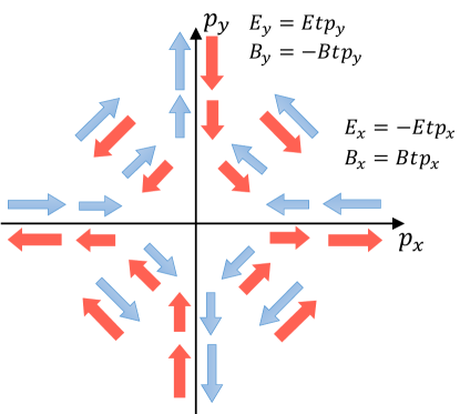
Figure 4: Configuration of the geometric electric and magnetic field (with $z=0$) in the momentum space. One can see the configuration becomes the same after $180^{\circ}$ rotation due to the spin-2 nature.

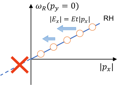
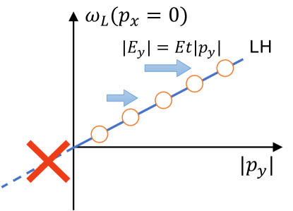
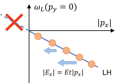
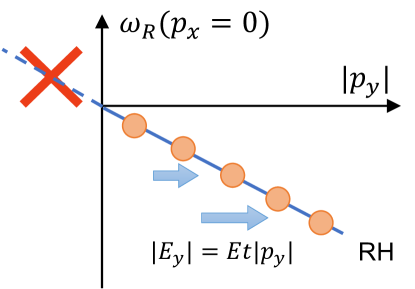
Figure 5: Schematic description that even if the LLL-like dispersion exists, positive mode and negative mode are not connected.

In Fig. 4, the configuration of “gravitational electric and magnetic field” of our metric (101) is shown in the momentum space (in the $p_{x}$-$p_{y}$ plane). Here the spin-2 nature is manifest such that the configuration becomes the same after $180^{\circ}$ rotation. This nature, however, results in the crucial difference from the case of U(1) gauge fields. Let us focus on the $p_{x}$ axis at $t\neq 0$ and $z=0$ where the geometric electric field and magnetic field are parallel to those axis,

$$B_{x}=Btp_{x},\quad E_{x}=-Etp_{x},\quad B_{y}=B_{z}=E_{y}=E_{z}=0.$$ (104)

In this axis, a simpler “kinematics” is expected. Since only the LLL participates the physics of the chiral anomaly in the U(1) case, the states we are interested in here would be those with spin aligned with the magnetic fields. On this axis, the magnetic field continues to point in the opposite direction for $p_{x}>0$ and $p_{x}<0$, namely, $\mathrm{sgn}(B_{x}(p_{x}>0))=-\mathrm{sgn}(B_{x}(p_{x}<0))$. Therefore one may expect the states similar to the LLL appear in a directionally dependent way. By naively applying the dispersion of LLLs (with the electric field being turned off), we anticipate the following LLL-like dispersion for these regions:

$$\omega_{\rm R}(p_{x}\neq 0,p_{y}=0) \simeq|p_{x}|,$$ (105)

$$\omega_{\rm L}(p_{x}\neq 0,p_{y}=0) \simeq-|p_{x}|,$$

where the $|p_{x}|$ dependence arises because of the flip of the geometric magnetic field direction at the origin of momentum space due to the spin-2 nature. Consequently, we find the LLL-like dispersion does not smoothly connect the negative and positive energy modes. Similar discussion holds for the $p_{y}$ axis. In Fig. 5, the dispersion (105) is schematically shown. Note that the direction of magnetic field and therefore the dispersion (105) does not change in time, but the Landau degeneracy per unit area, $|{\bm{B}}|/2\pi$, should change with time and momentum according to Eq. (103).

When the electric field is applied to the system for a certain time duration, the LLL allows the excitation continuously to occur in the case of U(1). As shown in Fig. 5, however, this spin-2 configuration does not seem to allow continuous level crossing on each axis in the same way as the U(1) example. That is, even if the LLL-like dispersion appears, it can not connect positive and negative frequency mode because of the $|p_{x/y}|$ dependence, and hence it is unlikely that particle production occurs even when we turn on the “electric” field. Although the geometric electric and magnetic fields are always aligned, absence of globally defined Landau-level in the present case, which is originated from the anisotropy and homogeneity, results in this qualitative difference. Moreover, at $p_{i}=0$ where $\omega_{\rm R/L}=0$ and the level crossing could occur, $E_{i}=0$ and hence no acceleration occurs. Having in mind that $h_{ij}$ interacts with fermions analogously to the $U(1)$ gauge field, we expect that the excitation cannot be the principal source for the fermion chirality.

Since we have non-vanishing $R{\tilde{R}}$, the anomaly equation should be totally satisfied by taking into account the vacuum contribution. Indeed, the second condition for the appearance of the vacuum contribution, namely, the asymmetric structure in the dispersion relation between the positive and negative energy modes, seems to be satisfied with non-zero $B$ independently for $p_{x}$ and $p_{y}$ axis. Although the contributions from the $p_{x}$ and $p_{y}$ axis looks to cancel each other for vanishing $E$, non-vanishing $E$ causes a bias in the opposite direction depending on the chirality (see Fig. 5), such that the cancellation is broken down. Therefore, we expect that an asymmetry would be accumulated as the vacuum contribution. Note that we have already seen that the first condition for the appearance of the vacuum contribution (gauge inequivalence of initial and final field configuration) is satisfied. Therefore, although we do not confirm that the anomaly equation is really satisfied by taking into account the vacuum contribution with a concrete calculation, we have the suggestion that all (or at least most of) the chiral charge would be accumulated in the vacuum. Note that we have a same situation in the Bianchi type-IX spacetime for $k<4$ discussed in Sec. 4.

Although the argument in the above is merely a qualitative discussion based on the kinematic analogy, we have obtained the suggestion for the inefficiency of the particle production through the level crossing in the case of parity-violating weak gravitational background with the field configuration (101). This behavior is totally different from the homogeneous U(1) case where the Landau level is globally defined and the electric field excites the field with the homogeneous acceleration. We have also seen that the case of Bianchi type-IX spacetime causes a weaker chiral particle creation through the level crossing along with a dominant vacuum contribution, but it is qualitatively different from our system. In that case, in addition to having non-Abelian-like interaction, which causes a bias term in the dispersion relation from the spin connection, the field configuration preserves the homogeneity of the system. We believe that this homogeneity leads to the less efficient but non-negligible amount of chiral particle production through the level crossing. In contrast, the spacetime with the geometric electric and magnetic field we considered in this section is highly inhomogeneous and anisotropic, which would be the reason of the inefficiency of the particle production. We emphasize that although more realistic field configuration must be considered to conclude, the features that lead to the inefficient level-crossing should be the same for the chiral GWs studied in the context of gravitational leptogenesis, which is nothing but the spin-2 perturbations around the conformally flat background. Therefore, we conjecture that the fermion chirality generated in the gravitational leptogenesis scenario is likely to be accumulated mainly in the vacuum.

We should admit that the above discussion is based on the naive application of the well-studied cases of gauge field, since we were not able to solve the field equation analytically. For example, we have not seriously considered the region where $p_{x}\cdot p_{y}\neq 0$ and the component of electric field that depends on $Bzp_{x/y}$. As we mentioned above, however, the latter contribution is hardly expected to be the essential contribution for generating chirality, because it is always orthogonal to the magnetic field (${\bm{E}}\cdot{\bm{B}}=0$). We also expect that chiral particle production may not efficiently take place in the region $p_{x}\cdot p_{y}\neq 0$ as the geometric magnetic field does not align with the momentum, resulting in low selectivity of chirality. One may think the field configuration we consider is not very good to examine the particle production in the gravitational leptogenesis, but we believe that it is the simplest field configuration that picks up its essential feature.

We would therefore expect the above inferences to be somewhat on target, but unfortunately they remain inconclusive yet. All these expectations could be clarified when, for example, the system is numerically solved. Before concluding, for our future reference, let us summarize the practical difficulties to work on the field equation of this system and the main differences from the solvable case of $U(1)$ gauge fields.

• Field configuration of $h_{ij}$ with $R\tilde{R}\propto EB$ results in the equation of motion where two directions of momentum are involved ($x/y$ in the above case).

• Since the order of derivative in $R\tilde{R}$ is different from that in $F\tilde{F}$ (second-order for the former while first-order for the latter), the geometric “electric” and “magnetic” fields in Eq.(103) have explicit space time dependence.

• The interaction between graviton and fermion non-trivially depends on the “momentum” of fermion field. This makes it difficult to solve the Dirac equation with the usual mode expansion of the fermion field if the globally defined momentum is absent.

5.3 Implication to the gravitational leptogenesis

Finally, let us comment on the feasibility of gravitational leptogenesis scenario in the light of our discussion in the above. As discussed in Sec. 2, chiral charge carried by the left-handed neutrinos, which is generated under chiral GWs during inflation, provides non-zero lepton number in the early universe. If sufficiently large lepton number is produced and converted into the baryon number, the observed baryon asymmetry could be explained by this anomalous contribution. As we have seen, however, it seems difficult for the parity-violating spin-2 gravitational field (including GWs) around the flat FLRW universe to cause level-crossing. Therefore, we have conjectured that the lepton number generated in this scenario (Eq. (4)) may almost coincide with the eta invariant and accumulate in the vacuum, which does not count the number of left-handed neutrinos as excited states.

If this is the case, one may wonder whether the transport relation (5) holds for the vacuum contribution. The relation (5) is derived under the framework of kinetic theory, which deals with the non-perturbative electroweak sphaleron process as well as the many body scattering in thermalized system. Therefore, it is questionable whether the lepton number accumulated in the vacuum can be converted into the baryon number in the thermal plasma according to Eq. (5) and contribute to the thermal history of the Universe such as the Big Bang Nucleosynthesis. If the lepton number accumulated in the vacuum, which may account for the substantial amount of net lepton number (4), completely decouples from this transport, resultant baryon-to-entropy ratio in this scenario could be significantly smaller than expected. Nevertheless, we cannot rule out the possibility that the “lepton-charged” vacuum induces a bias for the sphaleron process to convert the vacuum lepton charge to the baryon number in the plasma. We leave the investigation whether the vacuum contribution becomes relevant for the baryon number conversion to future work.

6 Summary and Discussion

In this paper, we investigated the chirality production of fermion under parity-violating spin-2 gravitational fields based on the existing studies on the cases with the gauge fields (e.g., Refs. Nielsen:1983rb ; Domcke:2018eki ; Domcke:2018gfr ). Chirality of fermion generally consists of the contribution from excitation and that accumulated in vacuum Atiyah:1963zz ; Atiyah:1968mp . The distinction of these contributions, however, was never addressed in the context of gravitational leptogenesis Alexander:2004us , where lepton number is produced by chiral GWs during inflation according to the gravitational chiral anomaly Kimura:1969iwz ; Delbourgo:1972xb ; Eguchi:1976db ; AlvarezGaume:1983ig . On the other hand, in addition to the old study on the Bianchi type-IX spacetime Gibbons:1979kq ; Gibbons:1979ks , the dominance of vacuum contribution was recently reported for the Bianchi type-II spacetime Stone:2023qln , both of which study parity-violating deformation of metric in the already-curved background. In this situation, it is worth investigating which contribution becomes dominant when the parity-violating spin-2 gravitational field is imposed around flat Minkowski spacetime. Such a clarification may help refining the prediction in the scenarios of gravitational leptogenesis.

We first made a review on the chirality generation under the gauge fields. While the smooth excitation in the LLL accounts for all the fermion chirality in the U(1) case, vacuum contribution known as eta invariant becomes important in the SU(2) case. The most distinct difference is that non-Abelian “magnetic field” causes overall bias in the dispersion similarly to the chemical potential, which makes the energy spectrum highly asymmetric, leading to the dominance of vacuum contribution in the chiral charge. As discussed in Sec. 4, this result is in fact helpful in understanding the generation of fermion chirality in the Bianchi type-IX spacetime, since it shares the similar characteristics with the homogeneous SU(2) gauge field case. To the best of our knowledge, this is the first discussion of this system from such a perspective, and the section can be considered as a comprehensive review, including an explicit decomposition into closed spheres and chiral GWs and confirmation of the APS index theorem. On the other hand, in both SU(2) and Bianchi type-IX cases, excited contribution in chirality is small but always non-negligible even in the strong external field limit. We conjecture that this behavior is provided by the homogeneity of the external field as it seems to allow continuous excitation.

In Sec. 5, we introduced a specific configuration of metric perturbation around the flat spacetime, which has the parity-violating spin-2 polarization and yields non-vanishing topological charge of the spacetime similarly to the aligned constant electric and magnetic field. With the classical analogy between the electromagnetism and weak gravitational field, we anticipate the physics of Landau levels in U(1) gauge field can be applied to the weak spin-2 gravitational system. The configuration in fact resembles the amplitude growth of chiral GWs, so it is appropriate for our purpose to discuss the chirality generation in the context of gravitational leptogenesis. However, as the order of differentiation in the curvature tensor differs, the metric perturbation admits non-trivial spacetime dependence in the Dirac equation, which acts as an anisotropic and inhomogeneous gravitational electric and magnetic field. As a result, it becomes difficult to obtain analytical solution and physical understanding of chirality generation. Thus we tried to investigate the system with brave approximations. That is, we assume that the system is described by the Landau levels induced by the geometric “magnetic” fields along which the fermions in the levels are accelerated by the geometric “electric” fields, in a similar way to the case of U(1) gauge field. From this approach, we find that the spin-2 nature of the gravitational field seems to prevent the efficient excitation. As the geometrical “magnetic field” changes the direction at the origin of the momentum space, smooth excitation could not take place in the “possible” lowest Landau level-like dispersion. If this investigation is correct for the gravitational leptogenesis, it may lead to less efficiency of the baryon number generation in the sceneario, since the charge transfer through the electroweak sphalerons to baryon charge is non-trivial for the lepton charge accumulated in the vacuum.

There are several directions in our future work. One direction is, of course, the numerical approach to the field equations we have formulated. Considering different configurations of the gravitational field than ours would also deepen the understanding of the effects of parity-violating gravitational fields. Moreover, we can think of alternative formulation of the system such as the chiral kinetic equation in curved spacetime Liu:2018xip ; Hayata:2020sqz . This theory naturally involves the extension of the momentum space and could be useful for our case where the momentum is regarded as the local quantity. If exist, it may be worth investigating whether the vacuum contribution of the induced energy momentum tensor can be renormalized or not similarly to the study of SU(2) gauge field case Domcke:2019qmm . Apart from the gravity, it is also worth addressing as a general question how chiral charges accumulated in a vacuum contribute to the transport equation as we mentioned in the last part.

References

- (1) S. L. Adler, Axial vector vertex in spinor electrodynamics, Phys. Rev. 177 (1969) 2426–2438.
- (2) J. S. Bell and R. Jackiw, A PCAC puzzle: in the model, Nuovo Cim. A 60 (1969) 47–61.
- (3) G. ’t Hooft, Symmetry Breaking Through Bell-Jackiw Anomalies, Phys. Rev. Lett. 37 (1976) 8–11.
- (4) N. S. Manton, Topology in the Weinberg-Salam Theory, Phys. Rev. D 28 (1983) 2019.
- (5) F. R. Klinkhamer and N. S. Manton, A Saddle Point Solution in the Weinberg-Salam Theory, Phys. Rev. D 30 (1984) 2212.
- (6) V. A. Kuzmin, V. A. Rubakov and M. E. Shaposhnikov, On the Anomalous Electroweak Baryon Number Nonconservation in the Early Universe, Phys. Lett. B 155 (1985) 36.
- (7) M. Fukugita and T. Yanagida, Baryogenesis Without Grand Unification, Phys. Lett. B 174 (1986) 45–47.
- (8) S. Y. Khlebnikov and M. E. Shaposhnikov, The Statistical Theory of Anomalous Fermion Number Nonconservation, Nucl. Phys. B 308 (1988) 885–912.
- (9) J. A. Harvey and M. S. Turner, Cosmological baryon and lepton number in the presence of electroweak fermion number violation, Phys. Rev. D 42 (1990) 3344–3349.
- (10) S. Y. Khlebnikov and M. E. Shaposhnikov, Melting of the Higgs vacuum: Conserved numbers at high temperature, Phys. Lett. B 387 (1996) 817–822, [hep-ph/9607386].
- (11) V. Domcke and K. Mukaida, Gauge Field and Fermion Production during Axion Inflation, JCAP 11 (2018) 020, [1806.08769].
- (12) V. Domcke, B. von Harling, E. Morgante and K. Mukaida, Baryogenesis from axion inflation, JCAP 10 (2019) 032, [1905.13318].
- (13) V. Domcke, K. Kamada, K. Mukaida, K. Schmitz and M. Yamada, Wash-in leptogenesis after axion inflation, JHEP 01 (2023) 053, [2210.06412].
- (14) M. Giovannini and M. E. Shaposhnikov, Primordial hypermagnetic fields and triangle anomaly, Phys. Rev. D 57 (1998) 2186–2206, [hep-ph/9710234].
- (15) K. Kamada and A. J. Long, Evolution of the Baryon Asymmetry through the Electroweak Crossover in the Presence of a Helical Magnetic Field, Phys. Rev. D 94 (2016) 123509, [1610.03074].
- (16) H. B. Nielsen and M. Ninomiya, ADLER-BELL-JACKIW ANOMALY AND WEYL FERMIONS IN CRYSTAL, Phys. Lett. B 130 (1983) 389–396.
- (17) M. F. Atiyah and I. M. Singer, The index of elliptic operators on compact manifolds, Bull. Am. Math. Soc. 69 (1969) 422–433.
- (18) M. F. Atiyah and I. M. Singer, The Index of elliptic operators. 1, Annals Math. 87 (1968) 484–530.
- (19) V. Domcke, Y. Ema, K. Mukaida and R. Sato, Chiral Anomaly and Schwinger Effect in Non-Abelian Gauge Theories, JHEP 03 (2019) 111, [1812.08021].
- (20) T. Kimura, Divergence of axial-vector current in the gravitational field, Prog. Theor. Phys. 42 (1969) 1191–1205.
- (21) R. Delbourgo and A. Salam, The gravitational correction to pcac, Phys. Lett. B 40 (1972) 381–382.
- (22) T. Eguchi and P. G. O. Freund, Quantum Gravity and World Topology, Phys. Rev. Lett. 37 (1976) 1251.
- (23) L. Alvarez-Gaume and E. Witten, Gravitational Anomalies, Nucl. Phys. B 234 (1984) 269.
- (24) S. H.-S. Alexander, M. E. Peskin and M. M. Sheikh-Jabbari, Leptogenesis from gravity waves in models of inflation, Phys. Rev. Lett. 96 (2006) 081301, [hep-th/0403069].
- (25) D. H. Lyth, C. Quimbay and Y. Rodriguez, Leptogenesis and tensor polarisation from a gravitational Chern-Simons term, JHEP 03 (2005) 016, [hep-th/0501153].
- (26) W. Fischler and S. Paban, Leptogenesis from Pseudo-Scalar Driven Inflation, JHEP 10 (2007) 066, [0708.3828].
- (27) A. Maleknejad, M. Noorbala and M. M. Sheikh-Jabbari, Leptogenesis in inflationary models with non-Abelian gauge fields, Gen. Rel. Grav. 50 (2018) 110, [1208.2807].
- (28) A. Maleknejad, Chiral Gravity Waves and Leptogenesis in Inflationary Models with non-Abelian Gauge Fields, Phys. Rev. D 90 (2014) 023542, [1401.7628].
- (29) S. Kawai and J. Kim, Gauss–Bonnet Chern–Simons gravitational wave leptogenesis, Phys. Lett. B 789 (2019) 145–149, [1702.07689].
- (30) R. R. Caldwell and C. Devulder, Axion Gauge Field Inflation and Gravitational Leptogenesis: A Lower Bound on B Modes from the Matter-Antimatter Asymmetry of the Universe, Phys. Rev. D 97 (2018) 023532, [1706.03765].
- (31) A. Papageorgiou and M. Peloso, Gravitational leptogenesis in Natural Inflation, JCAP 12 (2017) 007, [1708.08007].
- (32) P. Adshead, A. J. Long and E. I. Sfakianakis, Gravitational Leptogenesis, Reheating, and Models of Neutrino Mass, Phys. Rev. D 97 (2018) 043511, [1711.04800].
- (33) K. Kamada, J. Kume, Y. Yamada and J. Yokoyama, Gravitational leptogenesis with kination and gravitational reheating, JCAP 01 (2020) 016, [1911.02657].
- (34) K. Kamada, J. Kume and Y. Yamada, Renormalization in gravitational leptogenesis with pseudo-scalar-tensor coupling, JCAP 10 (2020) 030, [2007.08029].
- (35) M. Stone, P. Howland and J. Kim, Gravitational Landau levels and the chiral anomaly, J. Phys. A 57 (2024) 115401, [2307.06811].
- (36) G. W. Gibbons, Spectral Asymmetry and Quantum Field Theory in Curved Space-time, Annals Phys. 125 (1980) 98.
- (37) G. W. Gibbons, COSMOLOGICAL FERMION NUMBER NONCONSERVATION, Phys. Lett. B 84 (1979) 431–434.
- (38) L. P. Grishchuk, Amplification of gravitational waves in an istropic universe, Zh. Eksp. Teor. Fiz. 67 (1974) 825–838.
- (39) D. H. King, Gravity wave insights to Bianchi type IX universes, Phys. Rev. D 44 (1991) 2356–2368.
- (40) B. Mashhoon, Gravitoelectromagnetism: A Brief review, gr-qc/0311030.
- (41) L. Filipe Costa and C. A. R. Herdeiro, A Gravito-electromagnetic analogy based on tidal tensors, Phys. Rev. D 78 (2008) 024021, [gr-qc/0612140].
- (42) S. Alexander and N. Yunes, Chern-Simons Modified General Relativity, Phys. Rept. 480 (2009) 1–55, [0907.2562].
- (43) R. Jackiw and S. Y. Pi, Chern-Simons modification of general relativity, Phys. Rev. D 68 (2003) 104012, [gr-qc/0308071].
- (44) K. Landsteiner, Notes on Anomaly Induced Transport, Acta Phys. Polon. B 47 (2016) 2617, [1610.04413].
- (45) E. V. Gorbar, K. Schmitz, O. O. Sobol and S. I. Vilchinskii, Gauge-field production during axion inflation in the gradient expansion formalism, Phys. Rev. D 104 (2021) 123504, [2109.01651].
- (46) T. Fujita, J. Kume, K. Mukaida and Y. Tada, Effective treatment of U(1) gauge field and charged particles in axion inflation, JCAP 09 (2022) 023, [2204.01180].
- (47) V. Domcke, B. Mares, F. Muia and M. Pieroni, Emerging chromo-natural inflation, JCAP 04 (2019) 034, [1807.03358].
- (48) P. Adshead and M. Wyman, Chromo-Natural Inflation: Natural inflation on a steep potential with classical non-Abelian gauge fields, Phys. Rev. Lett. 108 (2012) 261302, [1202.2366].
- (49) N. H. Christ, Conservation Law Violation at High-Energy by Anomalies, Phys. Rev. D 21 (1980) 1591.
- (50) K. Fukushima, Y. Hidaka, T. Shimazaki and H. Taya, Chiral anomaly in a (1+1)-dimensional Floquet system under high-frequency electric fields, Annals Phys. 458 (2023) 169494, [2305.11432].
- (51) C. W. Misner, Mixmaster universe, Phys. Rev. Lett. 22 (1969) 1071–1074.
- (52) D. R. Brill and J. M. Cohen, Cartan Frames and the General Relativistic Dirac Equation, J. Math. Phys. 7 (1966) 238.
- (53) N. Hitchin, Harmonic Spinors, Adv. Math. 14 (1974) 1–55.
- (54) A. Vilenkin, MACROSCOPIC PARITY VIOLATING EFFECTS: NEUTRINO FLUXES FROM ROTATING BLACK HOLES AND IN ROTATING THERMAL RADIATION, Phys. Rev. D 20 (1979) 1807–1812.
- (55) D. T. Son and P. Surowka, Hydrodynamics with Triangle Anomalies, Phys. Rev. Lett. 103 (2009) 191601, [0906.5044].
- (56) K. Landsteiner, E. Megias and F. Pena-Benitez, Gravitational Anomaly and Transport, Phys. Rev. Lett. 107 (2011) 021601, [1103.5006].
- (57) N. D. Birrell and P. C. W. Davies, Quantum Fields in Curved Space. Cambridge Monographs on Mathematical Physics. Cambridge Univ. Press, Cambridge, UK, 2, 1984, 10.1017/CBO9780511622632.
- (58) L. E. Parker and D. Toms, Quantum Field Theory in Curved Spacetime: Quantized Field and Gravity. Cambridge Monographs on Mathematical Physics. Cambridge University Press, 8, 2009, 10.1017/CBO9780511813924.
- (59) Y.-C. Liu, L.-L. Gao, K. Mameda and X.-G. Huang, Chiral kinetic theory in curved spacetime, Phys. Rev. D 99 (2019) 085014, [1812.10127].
- (60) T. Hayata, Y. Hidaka and K. Mameda, Second order chiral kinetic theory under gravity and antiparallel charge-energy flow, JHEP 05 (2021) 023, [2012.12494].
- (61) V. Domcke, Y. Ema and K. Mukaida, Chiral Anomaly, Schwinger Effect, Euler-Heisenberg Lagrangian, and application to axion inflation, JHEP 02 (2020) 055, [1910.01205].