Comparing Multivariate Distributions: A Novel Approach Using Optimal Transport-based Plots
Abstract
Quantile-Quantile (Q-Q) plots are widely used for assessing the distributional similarity between two datasets. Traditionally, Q-Q plots are constructed for univariate distributions, making them less effective in capturing complex dependencies present in multivariate data. In this paper, we propose a novel approach for constructing multivariate Q-Q plots, which extend the traditional Q-Q plot methodology to handle high-dimensional data. Our approach utilizes optimal transport (OT) and entropy-regularized optimal transport (EOT) to align the empirical quantiles of the two datasets. Additionally, we introduce another technique based on OT and EOT potentials which can effectively compare two multivariate datasets. Through extensive simulations and real data examples, we demonstrate the effectiveness of our proposed approach in capturing multivariate dependencies and identifying distributional differences such as tail behaviour. We also propose two test statistics based on the Q-Q and potential plots to compare two distributions rigorously.
Keywords: Q-Q plots; multivariate quantile; optimal transport; entropy regularisation; hypothesis testing; geometric quantile; tail behavior
1 Introduction
Univariate Quantile-Quantile (Q-Q) plot is a graphical tool used in statistics to assess whether two samples follow a similar distribution by comparing their respective quantiles. It is a simple yet powerful visualization technique that provides valuable insights into the shape, location, and scale of two samples.
While the univariate Q-Q plot is well defined, there is not much literature on multivariate Q-Q plots. This perhaps can be attributed to the absence of natural ordering. Easton and McCulloch (1990) introduced a permutation based multivariate Q-Q plot, where samples of equal length are matched against each other such that the total distance between them is minimised. Subsequently, the corresponding components of matched samples are plotted against one another in different bivariate plots. These plots then show visual evidence of similarity of underlying distributions of the two sets of samples. In Dhar et al. (2014), the authors used the crucial property of unique characterisation of underlying distributions by geometric quantile to develope componentwise Q-Q plots. Specifically, samples are matched according to their geometric rank, and then a componentwise plotting of matched samples provides insight into the underlying distributions.
In this context, we aim at extending this graphical tool using the optimal transport (OT) map, to which we refer as OT Q-Q plot. We prove that, as the sample size increases, the Q-Q plots are concentrating around the straight line passing through the origin and with slope , if and only if the two sets of samples are drawn from the same distribution. This characteristic enables us to visually compare two distributions.
Moreover, in the context of very large dimensions, the componentwise plot may not be ideal due to a large number of bivariate plots. So, we suggest an alternative approach based on OT potential function, which allows for the comparison of two sets of multivariate samples in a single bivariate plot, named OT potential plot. Similar to the componentwise plots, we establish that, as the sample size increases, the potential plot becomes arbitrarily close to the straight line with slope and passing through the origin if and only if the underlying distributions of the two samples are identical.
Computing empirical OT maps can be costly, especially when sample sizes are large; see Hütter and Rigollet (2021). Therefore, practical solutions have been proposed in the literature, one of the most popular approaches being the entropy regularisation, introduced in Cuturi (2013). By selecting the regularisation parameter to be sufficiently small, the entropy regularised OT (EOT) map and EOT potential can closely approximate the OT map and OT potential, respectively. Moreover, we prove that the EOT map and EOT potential can also uniquely characterize the distribution.
These significant properties of EOT map and EOT potential serve as our driving force to also build Q-Q plots (we call it Q-Q, although EOT maps are not quantiles) and potential plots based on them. Finally, as given in Shapiro and Wilk (1965); Dhar et al. (2014), we propose test statistics to assess the relevance of the proposed Q-Q plots and potential plots.
We apply this (E)OT approach on examples from simulated and real data, then compare (E)OT Q-Q plots with geometric ones.
Our contributions are the following:
-
(i)
We construct OT Q-Q plots for comparing multivariate distributions, as we can prove that these plots are concentrating, as the sample size increases, around the straight line passing through the origin and with slope , if and only if the two sets of samples are drawn from the same distribution.
-
(ii)
We also propose OT potential plot, which is shown to share the same unique characterization property as for OT maps. This tool is quite interesting as it gives a single bivariate plot, whatever the dimension of the distribution.
-
(iii)
We develop the same tools and characteristic properties as for OT when considering the EOT approach, widely used because less computationally challenging than the OT approach.
-
(iv)
We propose test statistics to assess the relevance of the Q-Q and potential plots as tools for comparing multivariate distributions, for the EOT approach.
-
(v)
We question the benefit of using (E)OT Q-Q or potential plots, to retrieve specific features of the distributions considered, specifically in the tail. We do so via an extensive simulation study.
-
(vi)
We compare (E)OT Q-Q plots with geometric Q-Q plots developed in Dhar et al. (2014), on simulated and real data. We observe that the former is better performing visually in general (on our examples) than the latter to characterize tail distributions.
Notation: denotes the norm, the set of all probability measures on d with convex support, the usual inner product on d, and means that has distribution . implies that the measure is absolutely continuous with respect to the measure . The measure is assumed to be uniform on the open unit ball unless otherwise specified. is the set of all couplings with first marginal and second marginal , and . Let be a probability measure and be a measurable set with . Then define the probability measure such that for all measurable sets .
Structure of the paper: In Section 2, we briefly recall the concepts related to OT, EOT maps, and potentials, together with their connections to the multivariate quantile function. Section 3 includes discussions and results related to constructions of multivariate Q-Q plots and potential plots based on OT and EOT. In Section 4, we propose two test statistics and study their asymptotics. In Section 5, we illustrate our (E)OT approach on simulated samples to compare multivariate distributions on various scenarios and experiments. In Section 6, we apply the method on real data. In Section 7, we compare results obtained with geometric and (E)OT Q-Q plots, respectively, first on simulated data, then on real data.
2 Background and preliminaries on multivariate quantile and potential function
2.1 Optimal transport approach
The motivation for defining multivariate quantile through optimal transport arises from certain inherent properties of the univariate quantile functions. One key property of the univariate quantile function is its nondecreasing nature. Another compelling aspect is that any probability measure is the pushforward of the uniform measure on the interval by its quantile function. These two properties together uniquely characterize a quantile function; any function meeting these criteria must be a quantile. This property of transporting measure in high dimensions is at the heart of the theory of optimal transport and has a very rich literature (see Villani (2003, 2009), Santambrogio (2015) for an exhaustive review). In particular, the following theorem due to Brenier (1991) and McCann (1995), proves the existence and uniqueness of a map that pushes forward a measure to if is absolutely continuous with respect to the Lebesgue measure. Moreover, the map is the gradient of a convex function, i.e. . The property that can be written as the gradient of a convex function, is analogous to the monotonicity property of univariate quantile function.
Theorem 2.1
(Brenier–McCann) Let and be two probability measures on d. Assume that is absolutely continuous with respect to the Lebesgue measure. Then, there exists a convex function on d, which is almost everywhere unique up to an additive constant, such that pushes forward the measure to the measure , notationally . If is also absolutely continuous with respect to the Lebesgue measure, then is invertible and , where is the Fenchel–Legendre transform of . Additionally, if both and have finite second moment, then uniquely solves the Monge problem:
| (2.1) |
Let be the uniform probability measure on the unit ball and be any probabilty measure on d, then Theorem 2.1 ensures the existence of a unique monotone map (the gradient of a convex function), which pushes forward to . The following definition of multivariate quantile function is from Chernozhukov et al. (2017) with minor modification, as explained in Remark 2.4.
Definition 2.2
(OT quantile; Chernozhukov et al. (2017)) Let be the uniform probability measure on . The function defined by such that for a convex function , is defined as the OT quantile function of the probability measure .
Although the OT quantile is almost everywhere unique, the convex functions in Theorem 2.1 are unique up to additive constants. Therefore setting its infimum to will ensure their uniqueness.
Definition 2.3
(OT Potential; Chernozhukov et al. (2017)) Let be the uniform probability measure on the unit ball . A convex function satisfying and is called the OT potential of .
Remark 2.4
-
1.
Since any convex function on bounded open set is bounded below by a finite number we can subtract the infimum to satisfy the condition . This will ensure that the potential function is non-negative everywhere.
-
2.
In the definitions above, the fixed measure is assumed to be the uniform probability measure on the unit ball. However, one can choose a different reference distribution; for instance, in Chernozhukov et al. (2017), Hallin et al. (2021), is considered to be the spherically uniform measure. We refer the reader to (Ghosal and Sen, 2022, Remark 3.11) for discussion on the effect of choosing different reference measures.
Later in this paper, we will extensively use the following properties of both OT quantile and OT potential, which are a straightforward consequence of Theorem 2.1.
Properties 2.5
(Unique characterisation of measure) Let and be two probability measures. Then,
-
(i)
if and only if , where are OT potentials.
-
(ii)
if and only if , where are the OT quantiles.
Empirical OT quantile -
When a distribution on is supported on finite points (i.i.d. samples), the empirical quantile function can be defined in either of the following ways:
-
•
Discrete to discrete: In this case, the empirical quantile function is an optimal transport map between two sets of samples. Thus, clearly, the quantile function is supported on the finite sample, generated uniformly on .
-
•
Continuous to discrete or semi-discrete: In this case, the quantile function is the transport map between the uniform measure on and a finite sample. Therefore, the map is defined on the whole unit ball. See Chernozhukov et al. (2017) for more details.
For simplicity, we consider the discrete to discrete version of empirical OT quantiles; and refer the reader to Chernozhukov et al. (2017); Hallin et al. (2021); Ghosal and Sen (2022) for more properties on empirical OT quantiles.
For the purpose of this work, we shall consider i.i.d. samples with and with , being the uniform measure on . Then, we define the empirical measures corresponding to and as
| (2.2) |
Definition 2.6
(Empirical OT quantile; Hallin et al. (2021)) The empirical quantile function of the empirical measure with respect to the reference measure is a function such that
| (2.3) |
where denotes the set of permutations of the set .
Remark 2.7
Remark 2.8
Observe that the function is random, and is supported on the random set . Although in our notation the empirical OT quantile seems to depend only on the measure , note that it is defined with respect to a reference . In Hallin et al. (2021), instead of taking a random sample , the authors construct a deterministic grid on to define empical OT quantiles.
Remark 2.9
The map may not be unique. For example, let and , and note that, there are only two possible bijective maps from to and the cost remains the same for each of them. Therefore there are two possibilities for the map . However, since is a sample drawn from an absolutely continuous distribution , the event that is not unique has probability zero; see Hallin et al. (2021).
For the empirical OT potential, we will adopt the definition from Chernozhukov et al. (2017), where it is defined such that its gradient coincides with the empirical quantile function on its finite support. The definition is based on the dual formulation of the Monge problem (2.1).
Definition 2.10
Note that , when restricted to the set , coincides with the empirical quantile function .
Lemma 2.11
Let be an absolutely continuous probability measure with convex support. Let and be population and empirical quantile functions with respect to and , respectively. Then, for any compact set ,
Proof. Since is absolutely continuous, the quantile function is bijective. The inverse of the quantile is defined as the multivariate distribution function or OT distribution function and denoted by , i.e. . Similarly, the empirical distribution function is the inverse of the empirical quantile, i.e. .
Note that the support of is convex, is a homeomorphism between and interior of . Let . Then we can write,
which, combined with Proposition 2.4 in Hallin et al. (2021) and the fact that is uniformly continuous on compact sets, concludes the proof of Lemma 2.11.
Lemma 2.12
Assume that the support of is compact and the optimal transport map is a homeomorphism from the open unit ball to the interior of . Then, for any compact ,
where denotes the convergence in outer probability in the sense of van der Vaart and Wellner (1996).
Proof. It is a straightforward adaptation of the proof of (Chernozhukov et al., 2017, Theorem 3.1) developed for OT maps, to OT potentials.
2.2 Entropy regularised optimal transport
While the optimal transport map provides a meaningful definition of the multivariate quantile function, it comes along with practical challenges. Estimating the optimal transport for large samples is costly, with complexity for a sample size . Cuturi (2013) proposed an entropy regularised optimal transport (EOT), which closely approximates the optimal transport, and reduces the complexity to .
In the following, we shall briefly review the basic concepts and properties of EOT.
Given two measures and , a weak version of the Monge problem, known as the Kantorovich relaxation, is given by
| (2.5) |
where is the set of all couplings between and . Since is compact in the weak topology and the cost function is lower semicontinuous, therefore the existence of a minimiser to the Kantorovich problem is guaranteed (see (Villani, 2009, Theorem )), whereas the minimiser does not always exist in the Monge problem. Additionally, the Kantorovich problem has a unique minimiser, denoted by , whenever both and have finite second moment and is absolutely continuous with respect to the Lebesgue measure. Furthermore, the unique minimiser is supported on the graph of the OT map (Brenier map) between and . In particular, , where is the OT map and the convex function is the OT potential. Alternatively, we can write
| (2.6) |
where . This establishes link between OT map () and the solution of the Kantorovich problem.
We will now discuss the entropy regularised version of the Kantorovich problem, which is defined by adding an extra penalty in the cost function . Specifically, for and probability measures and which have finite second moment, the entropy regularised Kantorovich problem is defined as
| (2.7) |
where (the product measure) and is the the Kullback–Leibler divergence given by:
This problem is known to have a unique minimiser , as proven in (Nutz, 2022, Theorem ).
Now, we recall the relation between OT map and the Kantorovich solution in (2.6), and analogously define the EOT map. In particular, the EOT map is defined as the conditional expectation with respect to .
Definition 2.13
(EOT map; Pooladian and Niles-Weed (2022)) Let be any probability measure defined on d with finite second moment. Let be the uniform probability measure on . Consider , then the EOT map is defined as:
We shall now explore an alternative representation of the EOT map. Specifically, analogous to OT map, we observe that EOT map can also be represented as the gradient of some potential function (not convex in general). This is achieved in duality. The EOT problem (2.7) admits strong duality, shown in (Genevay, 2019, Theorem 7), in the following way: let denote the cost of the regularised version of the Kantorovich problem, i.e.
| (2.8) |
then,
| (2.9) |
If and have finite second moment, the maximiser of (2.9) is unique, –almost surely, up to an additive constant. More precisely, if is another pair of solutions to the dual Kantorovich problem, then there exists a constant such that and . Importantly, the EOT map can be expressed as the gradient of an EOT potential function (see Section 3 in Pooladian and Niles-Weed (2022)), i.e.
| (2.10) |
Definition 2.14
(EOT potential) Let be a maximiser of (2.9), where is the uniform probability measure on the unit ball and is any probability measure defined on d with finite second moment. Then the function defined by
where is a fixed point, is called the EOT potential corresponding to .
Remark 2.15
Whenever minimisers exist, we will set , which will ensure that the EOT potential is non-negative everywhere.
Now, we move to the unique characterisation property of EOT maps and potentials.
Proposition 2.16
Let be the uniform measure on the unit ball and , be two probability measures with finite second moment. Let be fixed.
-
(i)
Let and be EOT potentials corresponding to and , respectively. Then, if and only if for -almost every .
-
(ii)
Consider two EOT maps and corresponding to the measures and . Then, if and only if , for -almost every .
Proof: (i) If , the proof follows from the fact that the optimisation problem in (2.9) has a unique minimiser up to the addition of a constant.
Now let us prove the reverse implication by contradiction. Suppose for almost every and for some , but . Since any pair of EOT potentials satisfies the Schrödinger system (see (Nutz, 2022, Section )),
we have
| (2.11) |
where the second equality follows by replacing with . Then, the proof follows from (Nutz, 2022, Theorem ).
(ii) The proof is similar to (i) after observing that the EOT map can be written in terms of potential function, i.e. ( see (2.10)).
Let us now consider the empirical counterpart of EOT map and potential, which will be later used to develop Q-Q and potential plots.
Empirical EOT map and its convergence
Let and be two sets of i.i.d. samples drawn from and (the uniform measure on ), respectively. Let and be empirical measures induced from and , as defined in (2.2).
Definition 2.17
Remark 2.18
-
1.
Notice that, although the measure is supported on a finite set , the empirical EOT map is by default defined on . However, recall that the empirical OT quantile is defined only on sample points .
-
2.
If is supported on a compact set, then, for a fixed , the empirical function converges almost surely to as ; see (Goldfeld et al., 2023, Lemma ).
-
3.
Note that in Definition 2.17, the number of observations in and is the same. In the case of two different sample sizes, i.e. and with , we can similary define emprical EOT map and potential by replacing with in the definition.
3 Construction of multivariate Q-Q plots
Let and be two sets of i.i.d. samples generated from and , respectively, and generated from the uniform measure on . Consider and the empirical quantile functions with respect to the reference sample . For each and , define the set
| (3.1) |
where is the th canonical basis vector. Therefore is a subset of 2, where each element is a pair of the th components of the OT quantile functions and . Now consider the empirical optimal potentials and . Then, for , define
| (3.2) |
In Theorem 3.2, we show that, as increases, and become arbitrarily close to the straight line with slope and intercept if and only if . With this property, we can define the OT Q-Q plots and OT potential plots as follows:
Definition 3.1
Let be the -neighbourhood of the diagonal line , i.e.
| (3.3) |
Theorem 3.2
Let be probability measures, defined in d, with convex support, i.e. . Let and be two i.i.d. samples drawn from and , respectively. Let , where ’s are i.i.d. with common distribution . Then, if and only if one of the following holds
-
(i)
, for all compact and all .
-
(ii)
, for all compact and all , where is the outer probability, in the sense of van der Vaart and Wellner (1996).
Proof. (i) First assume . Then the corresponding quantile functions are also equal, . By the construction of the set (see (3.1)), it follows that, for any fixed ,
| (3.4) |
where and are discrete to discrete optimal transport maps from to and to , respectively. To prove the first part of the theorem, it is enough to show that the probability of the event in the right side of (3.4) converges to as increases to infinity. Now the sample quantile functions , converge uniformly to and , respectively (by Lemma 2.11), and by assumption, hence the result.
Conversely, assume that (i) holds for all and for any compact subset . Therefore, almost surely, converges to as goes to infinity. Now, the convergence of empirical OT quantile to its population counterpart (see Lemma 2.11) implies that . Since the random set is almost surely dense in the unit ball , and are continuous, thus . Now from Proposition 2.5, we conclude that .
(ii) If , the proof is similar to the first part of (i).
Conversely, assume that (ii) holds for all compact subsets and . Then we have,
| (3.5) |
Let . If , then .
If there exists some such that , choose a compact subset such that . Now,
| (3.6) | ||||
The last identity follows by the definition of the set . Since , it follows that .
This contradicts (3.5), hence . Now the proof follows from Proposition 2.5 .
Let be fixed and be such that and are non empty. Recall that is a reference sample drawn from the uniform distribution on . Let and be two empirical EOT maps (for the subsamples and , respectively), and and be two EOT potentials, as defined in Section 2.2. Then, for , define the sets,
| (3.7) |
and
| (3.8) |
Definition 3.3
Let be a compact set. An EOT Q-Q plot is a collection of individual scatter plots, where the –th one displays the set . Similarly, a scatter plot of the set is called EOT potential plot.
The next theorem proves similar results as in Theorem 3.2 but for EOT.
Theorem 3.4
Let and be two probability measures with finite second moment. Let and be two i.i.d. samples drawn from and , respectively. Let , where ’s are i.i.d. with common distribution . Then if and only if one of the following holds.
-
(i)
, for all compact and all .
-
(ii)
, for all compact and all .
Proof.
First assume that . Let be a probability measure obtained by restricting on the compact set . Similarly, be the restriction on . Then the potentials for the restricted measures are equal, i.e. .
Since both (random) empirical measures and converge (weakly) to the limit
almost surely, therefore Lemma of Goldfeld et al. (2023) implies that converges to almost surely, for any integer . Here,
defined as the usual Hölder norm with exponent . The proof now follows through a similar argument as employed in Theorem 3.2.
The proof is similar as for the first part, after observing that the map is continuous and linear from to .
4 Test Statistics for comparing two distributions
As in Shapiro and Wilk (1965); Dhar et al. (2014), we propose two test statistics which are motivated from our Q-Q plots. Consider the i.i.d random variables and with common distributions and , respectively, and assume the corresponding EOT maps as defined in Section 2.2. We can measure the total deviation of the EOT Q-Q plots from the straight line by the quantity . Similarly, the total deviation in the EOT potential plot can be measured by the quantity . Therefore, we define the following two test statistics
| (4.1) |
Since the supports of and are compact, it follows from (Goldfeld et al., 2023, Lemma ) that for any , , where is a constant depending on and the support of the measures , . In other words, the potentials and their derivatives are uniformly bounded on . This implies that and are almost surely finite for all .
Proposition 4.1
Let and be two probability measures supported on compact subsets of d. Let , and be two independent sets of samples drawn from and , respectively. Consider and as in (4.1), then we have
where and are non-negative random variables with finite variance.
Proof. The samples and are independent of each other, hence and are also independent. Therefore, it follows from (Goldfeld et al., 2023, Theorem ) that,
| (4.2) |
where and are i.i.d mean zero Gaussian random elements, taking values in the space . Observe that the map is continuous from to , for any . Hence, . Therefore, by Fernique’s theorem, we have .
The result follows by an application of the functional delta method, as proven in (Goldfeld et al., 2023, Corollary ). A similar line of argument holds for .
We can then deduce the following theorem from Proposition 4.1.
Theorem 4.2
Assume that and are two probability measures with compact support. Consider the null hypothesis and the alternate hypothesis . Let and their limits be defined as above, with and non-degenerate. Then the following holds:
-
(i)
For and the -th quantile of , we have,
and
-
(ii)
For and the -th quantile of , we have,
and
Proof.
-
(i)
Corollary in Goldfeld et al. (2023) implies that, under the null hypothesis, converges in distribution to . Therefore, we have .
Moving to the second part of the statement, first note that
Therefore,
Now, notice that, under ,we have . Further, it follows from Corollary in Goldfeld et al. (2023) that:
-
•
and
converge in distribution to some random variables with finite variance; -
•
converges to zero almost surely.
Combining all these observations, we conclude that , from which we deduce the second statement.
-
•
-
(ii)
The proof of this part follows similarly as in part (i).
Remark:
-
1.
For the OT maps and OT potentials, the asymptotic limit theorems are not known in full generality. Whereas, in case of EOT, the limit theorems are proven in Goldfeld et al. (2023). This is why we provided the test statistics only through EOT maps and EOT potentials. Nevertheless, once limit theorems known in the OT case, test statistics can be defined for OT maps and potentials in the same way as we did for EOT.
-
2.
Note that the variances of the limiting random variables and are finite, but not known explicitly. This is why we evaluate them numerically in the examples given in Section 5.
5 Experimental design on simulated data
In the preceding sections, we defined Q-Q plots and potential plots, for both OT and EOT approaches, and established the requisite theory to assess if two given sets of multivariate samples originate from a same distribution. In this section, we test how these theoretical results apply in practice, and check the effectiveness of the visual tools offered by OT and EOT plots on various simulated data. To this aim, we perform four first experiments, considering two samples drawn from distributions such that: (I) they are identical; (II) they have different dependence structures; (III) they are related by a scaling map; (IV) one of them exhibits outliers. Thereafter, we consider the same question, but now focusing on the tail of the distribution. Note that the potential function which gradient pushes forward a regularly varying (RV) probability measure into another regularly varying (RV) probability measure, is also (under some conditions) regularly varying; see (de Valk and Segers, 2018, Theorem 5.1). Can we clearly distinguish between light and heavy tails with these (OT, EOT) Q-Q and potential plots, like in the case of geometric quantiles (or univariate quantiles)? To answer this question, we proceed to two additional experiments, where we compare multivariate Gaussian distribution with two different heavy-tailed distributions. All scenarios in the following examples are developed considering i.i.d and non i.i.d distributions.
More formally, using our previous notation, for each experiment, we proceed as follows:
-
(i)
Consider two samples, and of size each and a compact set . In all the experiments we choose such that ;
-
(ii)
Draw another sample from the uniform distribution on , which serves as a reference for comparison. Let be a compact set. In all the experiments we choose such that ;
-
(iii)
Q-Q plots: build the sets , , for the OT Q-Q plot and for the EOT Q-Q plots;
-
(iv)
Potential plots: build for the OT potential plot and for the EOT potential plot;
-
(v)
Examine if the Q-Q and potential plots concentrate around the straight line denoted by with slope and intercept ;
-
(vi)
If they do, infer from Theorems 3.2 and 3.4 that the samples share the same distribution. Otherwise, look for any discernible pattern present in the scatter plots and whether this pattern may unveil any distinct features. For instance, observe if the points appear to cluster around any specific nonlinear curve (see Figure 9);
-
(vii)
Estimate the values of the test statistics and , and estimate the corresponding p-values, to statistically assess the conclusions drawn from the plots. Note that the p-values are meaningful only when comparing distributions supported on compact sets, as Theorem 4.2 is applicable to compactly supported distributions. However, when dealing with fully supported distributions, a partial analysis can be conducted by restricting them to a large enough compact set. Two Borel probability measures are considered identical if and only if their restrictions across all compact sets are identical.
-
(viii)
Finally we also study numerically the role of the regularisation parameter for EOT.
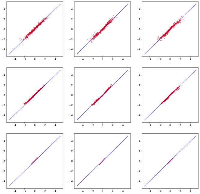
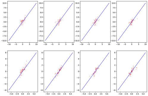
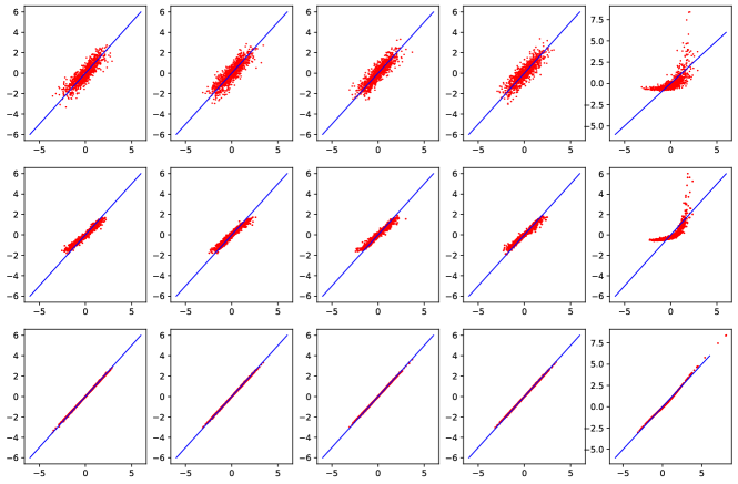
In the following examples, we present two kinds of plots: Q-Q plot and potential plot. In each Q-Q plot example, we display the OT and EOT Q-Q plots together in a single frame: the first row for OT and the second for EOT. In each plot, the -axis corresponds to the first sample and the -axis to the second sample . Also, the potential plots are presented together in a single frame: the left for OT and the right for EOT. Please note that all computations are performed using the POT (Python Optimal Transport) package; for detailed documentation, we refer to Flamary et al. (2021).
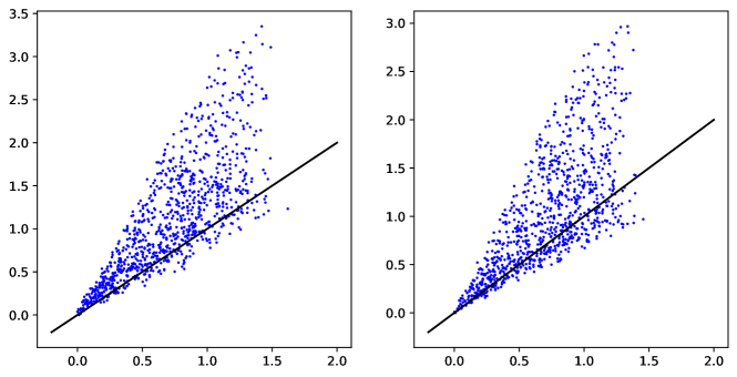
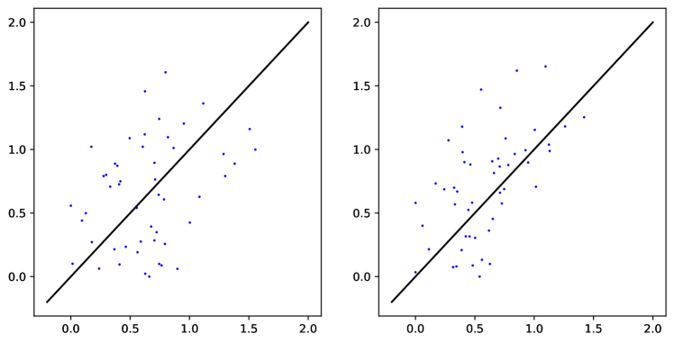
5.1 Example: Comparison between two samples drawn from a multivariate (non i.i.d.) Gaussian distribution
Starting with step (i), we consider two sets of i.i.d. samples, and , drawn from distributions and , respectively, where is a trivariate normal distribution with mean zero and covariance matrix , where, for instance, , , and . The number of observations in each sample is . Following steps (ii) to (iii), we obtain the OT and EOT Q-Q plots for these two samples, as displayed in Figure 1.
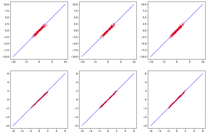
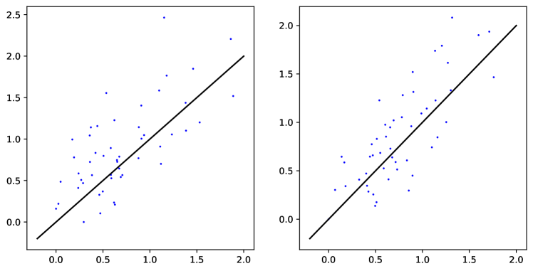
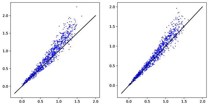
Next, we provide the potential plots for this example following the step (iv); see Figure 2. Note that for EOT, we choose .
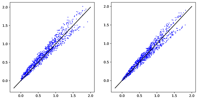
As expected, we observe that, for both types of comparisons, Q-Q and potential ones, the scatter plot is concentrated along the line . Therefore, according to step (vi), we can infer that the two samples are drawn from the same distribution. Although the spread around the straight line appears larger in the case of potential plots than in Q-Q plots, notice that the two sets of plots are shown on different scales, and that the dispersion in absolute terms is comparable in both cases.
A relatively larger spread is observed in the extremal regions of the potential plots, which may be ascribed to poorer approximation of the potential function in the extreme region when having fewer observations.
Compared to the OT plots, we also observe sharper clustering around the straight line in case of EOT. A possible reason for this could be that EOT maps and potentials are more regular than their OT counterparts (Nutz (2022)).
Next, we perform statistical test checking the similarity of the underlying distributions of the two samples and . We set the null hypothesis as , and empirically estimate the values of the test statistics and defined in (4.1). Additionally, the limiting distributions of and are empirically estimated, from which we deduce the -values under . We will proceed in the same way in all the illustrations. The values of the test statistics and -values are reported in Table 1, varying the sample size . Since the -values are relatively high, whatever the sample size, it supports the assertion that the two samples have originated from the same distribution.
| -value of | -value of | |||
5.2 Example: Characterising dependency
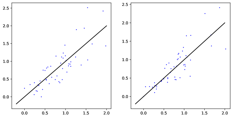
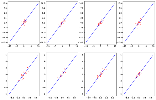
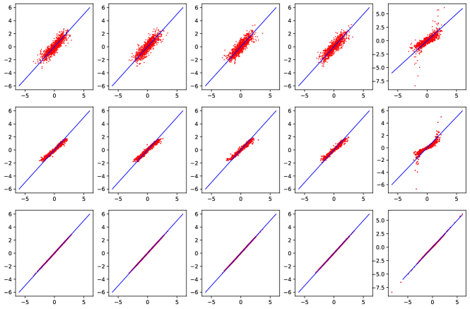
In multivariate setting, assessing dependency among marginals is an essential feature of multivariate statistical analysis. In this experiment, we compare two samples, one drawn from a distribution with independent marginals against one drawn from a distribution having dependent marginals, to see if there is any specific feature that can be observed from the Q-Q and potential plots. We consider two samples; the first one is drawn from (), a trivariate standard normal distribution, and the second from (), a normal distribution with zero mean and covariance matrix , where , , and . The Q-Q and potential plots are displayed in Figures 3 and 4, respectively.
In both Q-Q plots (OT and EOT), we observe that, although the points are concentrated along the line , the concentration is stronger for the third component (especially for EOT), as compared to the plots for the first and second component. Since the second distribution exhibits a high correlation () between the first and second marginals, would this pattern indicate some dependence? Answering this question will require further research and experiments, considering various dependence structures.
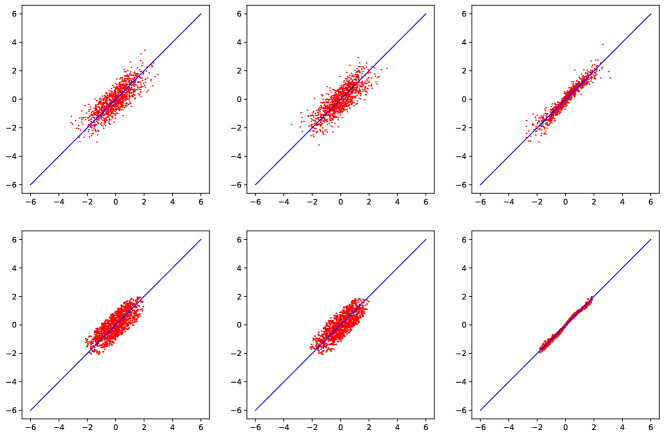
Turning to potential plots displayed in Figure 4, we can assess that the samples considered for the experiment have originated from different distributions. However, we cannot deduce any specific pattern in the plots that would suggest a high dependence among some components. Here too, further research needs to be developed.
Finally, we empirically estimate the values of the test statistics and defined in (4.1), as well as the corresponding -values under . The values are reported in Table 2. The small -values lead to the statement that the two samples have originated from two different distributions.
| -value of | -value of | |||
Observe that the values of and are getting larger as the sample size increases. This may indicate that the two underlying distributions are not the same, since we know that and tend to infinity in such a case. Also note that the -values are exactly zero, which looks too good to be true. Although the limiting distributions of and are fully supported on the positive real line, our approximations of those are supported on bounded sets. Therefore, the large values of and , which correspond to small probability regions of the limiting distributions, easily fall beyond the support of the approximated limiting distributions. To obtain non-zero -values, either the approximations have to be more accurate so that their supports are large enough to contain and , or the limiting distributions have to be known precisely.
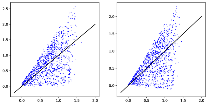
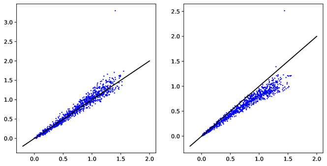
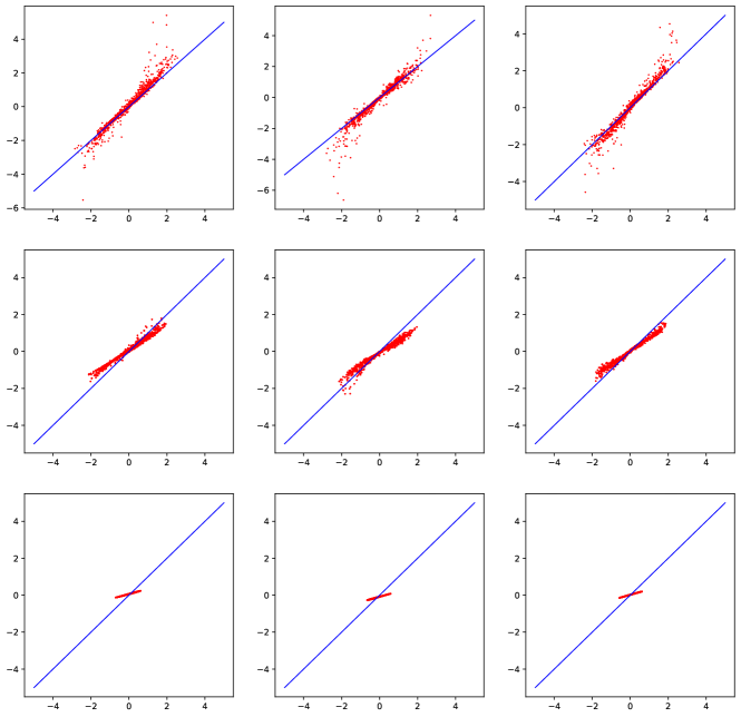
5.3 Example: Gaussian versus scaled Gaussian
We draw samples from , a standard normal distribution and from , a centered normal distribution with covariance matrix . The Q-Q plots are displayed in Figure 5. We observe that in the first and third columns in both rows, the points are concentrated around the line with slope (blue line) whereas in the second column, the points are concentrated around the line with slope (black line). This observation suggests that , indicating that the second distribution differs from the first by a scaling factor represented by the matrix . Since is set very small , the entropy regularised quantiles closely approximate , and as a result, we see that in the second plot of the second row, the points are also approximately concentrated around the straight line with slope (black line). However, it is important to recall that the EOT map is not necessarily scale equivariant in general.
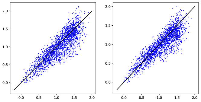
We present potential plots (left for OT and right for EOT) for the same pair of samples and in Figure 6. Clearly, the scatter plots are spread out and not concentrated along the straight line . This observation suggests that the underlying distributions corresponding to the two samples are not identical. But, unlike the Q-Q plots (shown in Figure 5), the potential plots do not offer additional information about the underlying distributions, such as the scaling in the sample .
Finally, we empirically estimate the values of the test statistics and defined in (4.1), as well as the corresponding -values under . The values are reported in Table 3. Since the -values are relatively small, this supports the assertion that the two samples have originated from distinct distributions.
| -value of | -value of | |||
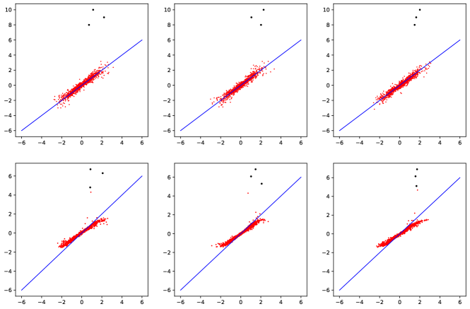
5.4 Example: Outlier Detection
We show that outliers can be detected using OT and EOT Q-Q plots. We illustrate this with two simulated samples, and , drawn from trivariate standard normal distributions, each containing 1000 observations. Subsequently, we replace three observations in with outlier points , , and , resulting in the transformed set . We follow steps (ii)–(iii) to build the Q-Q plots for and , and display them in Figure 7. The three black points, which are far from the rest of the observations, clearly reveal the presence of outliers. Next, we present the potential plots (step (iv)) for these two samples in Figure 8.
Notice that, although there are outliers present in the second sample, we only see one outlying point in the potential plot (compare this with Q-Q plots in Figure 7). It appears that potential plots may be less informative in this case compared to the Q-Q plots.
It is worth noticing that we set the value of the regularisation parameter as in this example, whereas in previous examples, we chose a larger value of . We observe that, with a higher value of , the EOT Q-Q plots do not distinctly separate the outliers. We shall study empirically the role of the regularisation parameter in visual analysis in Subsection 5.6.
5.5 Example: Light tail vs Heavy tail
To compare the heaviness of tail distributions, we provide a first example in dimension considering two distributions: the standard normal distribution (for the light tail) and the Student’s –distribution (for the heavy one). Another example comparing the trivariate standard normal distribution with i.i.d. Pareto() marginals can be found in Appendix A.
Recall that the density of the Student’s –distribution in dimension is given by
| (5.1) |
where , is a symmetric positive semidefinite matrix and is the gamma function. The parameter determines the heaviness of the distribution in the sense that moments of order greater than are infinite. We follow step (i) and draw a sample of size from the trivariate standard normal distribution . Similarly we draw of the same size from a trivariate Student’s –distribution, with parameters , (identity in 3) and . We go through steps (ii)–(iii), and display the Q-Q plots in Figure 9.
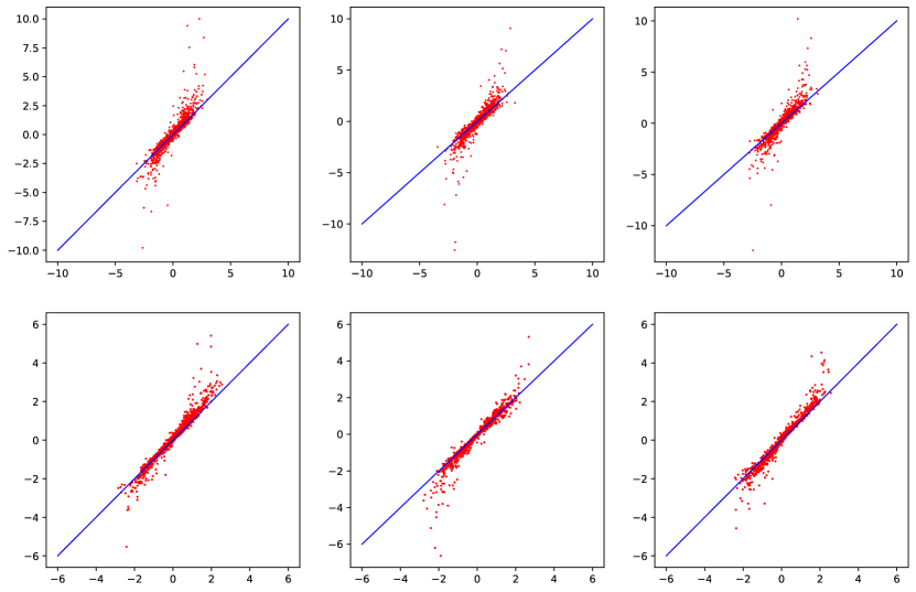
Here, we observe that the OT and EOT quantiles for grow at a faster rate than those of . The peculiar shape (S-shape) of the scatter plot seen in Figure 9 is very familiar in the univariate Q-Q plots involving heavy vs light tail comparisons. This hints at a similar behaviour in the OT plots. This feature, which is very useful in the univariate analysis, needs further exploration in the (E)OT setting.
| -value of | -value of | |||
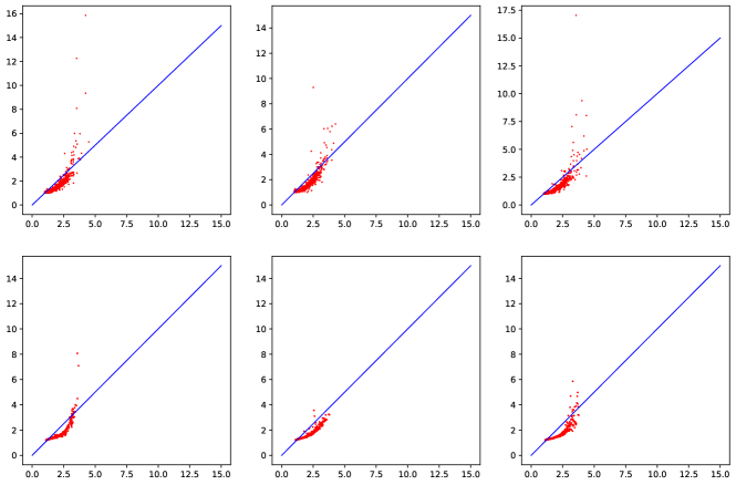
We then present potential plots (step (iv)) for this particular example in Figure 10. It can be seen from the plots that the points are scattered around a nonlinear (increasing) curve above the line . This implies that the potential function associated with the second sample has a higher growth rate. Since the (E)OT maps are gradient of (E)OT potentials, a higher growth rate of potential implies that the corresponding distribution has a heavier tail than that of first one.

The -values corresponding to and are provided in Table 4, although not so informative given the question on tail behaviour.
5.6 The effect of the regularisation parameter in EOT
As stated in Proposition 2.16, both EOT map and potential uniquely characterise distributions, regardless of the value of the regularisation parameter . However, the regularisation parameter plays an important role in the visual analysis. For a reasonably small value of (depending upon the distribution), the EOT map and potential closely approximate the OT map and potential, respectively. As a consequence, the EOT plots (Q-Q and potentials) look very similar to the OT plots (Q-Q and potentials); see for e.g. Figures 1–6.
On the other hand, the EOT map (resp. potential), with a large value of , is far from being a close approximation of the OT map (resp. potential).
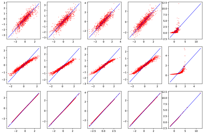
Taking back the setup of Example 5.1, we compute and display in Figures 11 and 13, respectively, the EOT Q-Q plots and potential plots when varying . We consider three values of : and , respectively. We observe that points are not only scattered around the line , they also begin to concentrate around a point on the line as the value of increases.
Recall that, as increases to , the EOT map converges to a constant map, with the constant being the mean of the target distribution. Therefore, for larger (e.g., in this case ), the EOT map is close to a constant, resulting in concentration around a point in the Q-Q plot. We next consider the same samples as in Example 5.5. We display the EOT Q-Q plots in Figure 12, for three different values of , and , respectively. Observe that, although the points are deviating from the line , which indicates that the two samples are non similar, they do not reveal the tail heaviness (compared with Example 5.1).
Therefore, for a large value of , while the EOT Q-Q plot can distinguish samples from different distributions, it may not reveal specific details such as the heaviness of the tails.
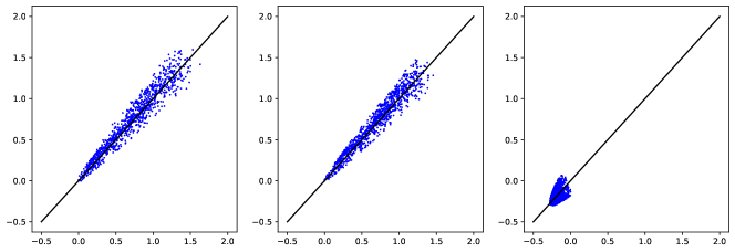
Let us now discuss the EOT potential plots for different values of . We first consider the setup in Example 5.1, let both samples are drawn from a trivariate standard normal distribution. We display the EOT potential plots in Figure 13, for three different values of , and , respectively.
Observe that, for large values of , the plots are not convincing enough to infer that the two sets of samples are generated from the same distribution.
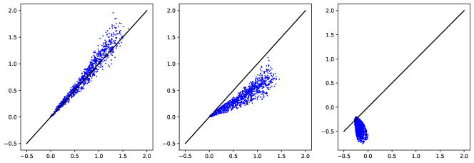
We show another example of potential plots in Figure 14. The samples are the same as in Example 5.5. Observe that, although the plots for each value of suggest that the samples are not very similar, it is difficult to infer visually (especially when is large) that one of the samples has a heavier tail than the other (Unless the EOT plot is very close to the OT one as in Figure 10).
It seems therefore ideal to choose small values of for better visual analysis. Nevertheless, it is important to note that smaller the value of , longer the algorithm takes to converge. Moreover, if is chosen too small, the algorithm (Sinkhorn) need more iteration to converge.
5.7 Key takeaways
-
(i)
We observe that both (OT and EOT) Q-Q plots and potential plots can efficiently identify the similarity between distributions. We experiment this with i.i.d and non i.i.d Gaussian distributions.
-
(ii)
When the samples are generated from a same distribution (in our example, a Gaussian distribution) with one of them having a scaling or shifting, we can identify this effect with Q-Q plots. Potential plots do not identify the shift, but the scale.
-
(iii)
We have shown with some examples that outliers can be detected with OT Q-Q plots and potential plots. For EOT, one needs to choose the value of the regularisation parameter to be small enough to observe them.
-
(iv)
Considering two examples, we showed that both Q-Q and potential plots can be used as a visual tool to compare tail distributions. For instance, comparing a light tail sample (e.g. Gaussian sample) with a heavy tail one (e.g. multivariate Student’s t-distribution), we could identify on the plots the heaviest tail between the two distributions.
-
(v)
When comparing distributions in high dimension, potential plots give a -dimensional representation, while a large number of componentwise plots is needed in the case of OT (and also geometric) Q-Q plots. As such, potential plots can be very useful in applied fields, e.g. risk management, as they offer:
-
–
A discriminating tool between light and heavy tail,
-
–
A visual validation tool for multivariate modelling.
-
–
Given these characteristics, to compare visually two multivariate distributions, we would recommend to proceed as follows:
-
1.
Plot the potential function to detect if the two samples are drawn from a same multivariate distribution;
-
2.
To obtain the whole comparison with specific features, consider the (E)OT Q-Q plots.
As a last remark, if comparing two samples which one suspects to come from a same family of distributions, then one may standardize the data to compute the (E)OT potential and Q-Q plots.
6 Application on real data
In the previous section, we considered many scenarios and experiments with simulated samples to have a better understanding of (E)OT Q-Q and potential plots as a visual tool to compare multivariate distributions. Now, we can turn to applications on real data. We consider two examples.
The first example is the Fisher’s Iris dataset, which can be downloaded from
https://archive.ics.uci.edu, a standard dataset used in statistics. It was also considered in Dhar et al. (2014) for analysing multivariate Q-Q plots based on geometric quantile, giving us a way to compare the results obtained when choosing two types of multivariate quantiles (see Section 7). The dataset has variables, and observations for each of the variables. Due to the relatively smaller size of this dataset, we consider another example offering a larger sample size. This second example is the Turkish rice Osmanic dataset, downloaded also from the link
https://archive.ics.uci.edu. It has variables, and observations for each of the variables.
6.1 Example 1: Fisher’s Iris data
This Fisher’s Iris dataset is constituted of three multivariate samples corresponding to three varieties: Iris Setosa, Iris Versicolour and Iris Virginica. Each variety consists of observations and each observation contains the measurement of variables, namely: sepal length, sepal width, petal length and petal width. Therefore, each sample is -dimensional with a size of . Following the steps (ii) to (iv) described in Section 5 to build the (E)OT potential and Q-Q plots, we compare each of the three samples with a 4-dimensional Gaussian sample of size 50. This choice of comparison is also motivated by the fact that Dhar et al. (2014) showed a strong evidence of normality of those samples using the geometric Q-Q plots. For a fair comparison, we follow the procedure of standardising the dataset, like in Dhar et al. (2014), before computing various quantiles and potentials. With the (E)OT approach, we obtain the potential plots displayed in Figure 15 for the three varieties of iris, and the Q-Q plots in Figure 16, for the Iris Setosa, Iris Versicolour, and Iris Virginica, respectively. Note that we also computed the associated test statistics and -values but choose not to report them here, as they heavily rely on the asymptotics of the test statistics, which is not compatible with such a small sample size. Looking at the potential plots, we observe that the points are very much spread out, which would hint at non–Gaussianity of the samples (Iris Setosa, Iris Versicolour and Iris Virginica). However, as already pointed out, the sample size is very small for any reasonable inference.
Iris Setosa data
Iris Versicolour data
Iris Virginica data
We now look at the (E)OT Q-Q plots, to compare the data with a multivariate standard Gaussian distribution. In Figure 16, for each of the three samples, the points are loosely concentrated around the straight line in the OT Q-Q plots, while in EOT Q-Q plots, they appear a bit more concentrated around the line .
Iris Setosa data
Iris Versicolour data
Iris Virginica data
6.2 Example 2: Turkish rice Osmanic data
In this second example, we consider the Turkish rice Osmanic dataset of size , with 5 variables that correspond to some features of the rice: Perimeter, Major Axis Length, Minor Axis Length, Convex Area, and Extent.
As previously, we want to compare the 5-dimensional standardised empirical distribution of this data with a -dimensional standard Gaussian distribution.
We draw the (E)OT potential plots (see Figure 17), followed by the (E)OT Q-Q plots (see Figure 18). For the EOT approach, we choose the regularisation parameter to be .
Looking at Figure 17, we observe that the points are spread out around the line (not as concentrated along as e.g. in Figure 13). So, we would deduce that the underlying distribution of the rice sample may not be well modelled by a multivariate standard Gaussian distribution. Let us move to the Q-Q plots in Figure 18 to gain more visual insights.
There, both OT and EOT Q-Q plots clearly indicate that the rice sample is drawn from a non-Gaussian distribution. Moreover, we observe a heavy tail behavior, for each component.
Since the sample size is reasonable, let us complete this empirical analysis by computing the test statistics and (defined in (4.1)) and the corresponding -values under the null hypothesis that the measure of the data (denoted ) is Gaussian (denoted ), i.e. .
| -value of | -value of | |||
The –values reported in Table 5 are small, as we could expect from what we observed on the various plots. This supports the assertion that the Turkish rice Osmanic data does not come from a Gaussian distribution.
7 Comparison with geometric Q-Q plot
In this section, we aim at comparing the QQ-plots as graphical tools (to compare two distributions) when adopting two main approaches, the (E)OT one and the geometric one. To do so, we display the OT, EOT, and geometric Q-Q plots for various simulated and real datasets, then, focus on comparing if one of the methods provides more informative or stronger visual insights about the two datasets being compared. For the procedure regarding geometric Q-Q plots, we refer the reader to Dhar et al. (2014).
7.1 Simulated data
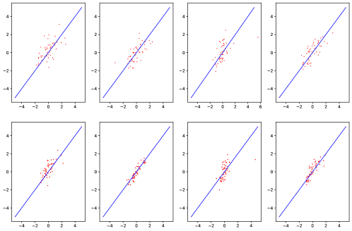
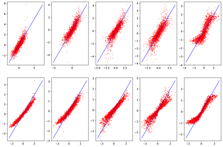
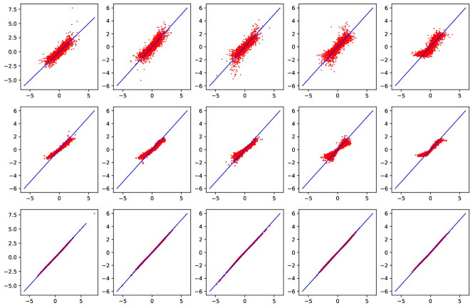
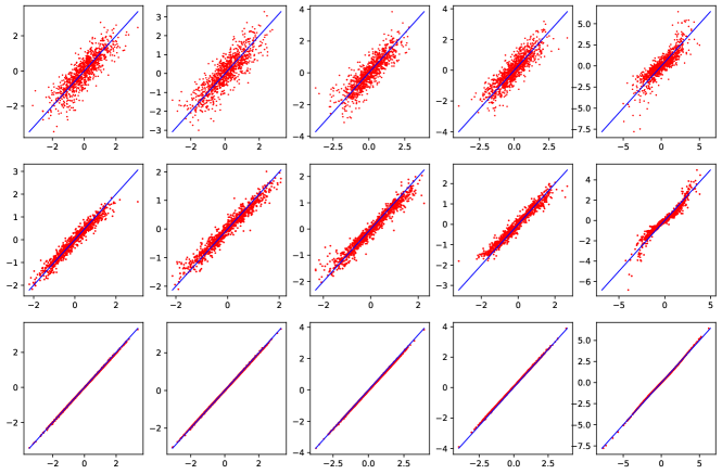
We begin by considering two sets of samples, each containing 1000 observations. The first set is drawn from a 5-dimensional standard Gaussian distribution, while the second set is drawn from a 5-dimensional distribution, chosen as follows. The marginals are independent, with the first four following a univariate standard Gaussian distribution, and the fifth one following a univariate Pareto distribution with parameter . In Figure 19, we depict types of multivariate Q-Q plots: the first row represents the OT Q-Q plots, the second row shows the EOT Q-Q plots when taking , and the last row displays the geometric Q-Q plots.
We observe in Figure 19 that OT and EOT Q-Q plots clearly reveal the presence of a heavy tail for the th component, whereas it is not so obvious from the geometric one. In the 5th component of the geometric Q-Q plot, we see some slight movement away from the straight line , but very mild in comparison with the OT and EOT approaches.
Next, we perform a similar experiment but replace the 5th marginal distribution for the second sample by a Student’s -distribution with degrees of freedom. The OT, EOT, and geometric Q-Q plots are displayed in Figure 20.
We observe that, while the OT and EOT Q-Q plots reveal the presence of heavy tails in the second distribution, the geometric Q-Q plot does not. Moreover, in the latter case, the point cloud becomes highly aligned with the straight line , suggesting that the two samples are drawn from the same distribution.
7.2 Real data
Here, we go back to Example 6.2, choosing the Turkish rice Osmanic dataset as second sample, while the first one is drawn from the -dimensional standard Gaussian distribution.
We note that both OT and EOT Q-Q plots indicate that the second sample is drawn from a distribution that is different from the Gaussian distribution. Additionally, we observe distinct tail behavior in the third and fifth components. However, the geometric Q-Q plot fails to differentiate between the two samples.
In Appendix B, we perform a similar comparison, but now comparing the unaltered real data with a multivariate Gaussian distribution whose parameters are learned from the data.
8 Conclusion
In recent times, multivariate OT based quantiles have become a very important object of research because it reflects many useful theoretical properties of univariate quantiles. Although OT is well understood theoretically, it is computationally very challenging for a large sample; it lacks statistical stability. Many possible solutions have been proposed to circumvent these issues, entropy regularisation (EOT) being one of them.
In this setting, considered both OT and EOT (maps and potentials) and obtained theoritical results that show that these (E)OT tools can be used to characterise distributions uniquely. Based on this property, we built multivariate Q-Q plots and potential plots by which one can visually compare two multivariate distributions.
(E)OT potential plots are interesting visual tools when comparing multivariate distributions, as they provide a -dimensional representation, which is an advantage w.r.t. Q-Q plots, especially in high dimension. However, Q-Q plots provide a visual comparison for specific features (scaling, shifting, outliers, tail heaviness) which is more obvious and readable than potential do.
Now, comparing OT versus EOT approach, we could observe that EOT Q-Q plots, with small regularization parameter, can determine well if two distributions are statistically similar or not, but they do not reveal informations about special features such as tail heaviness. Note that it is important to choose the value of sufficiently small so that the EOT map closely approximates the OT map, otherwise, for big values of , the EOT map becomes close to a constant map. It is also observed that the smaller the values of , the longer the algorithm takes to execute. Also, if is chosen very small, it happens sometimes that the code in Flamary et al. (2021) breaks down because of encountering NaN value.
Finally, we proposed statistical tests associated with the EOT Q-Q and potential plots, based on the available statistical stability results (central limit theorems) for EOT. Once limit theorems will be available for OT, we will be able to construct test statistics for OT as well, in a similar way as for EOT. Note that limit theory for OT is an area of active research, for recent developments on this topic, we refer e.g. to Sadhu et al. (2023); Manole et al. (2023).
Our future goal is to study the asymptotic of empirical estimators of the (E)OT quantile and potential function, specifically their tail behavior, as we did for geometric quantiles and half-space depths (see Singha et al. (2023)). It will be helpful to have a better understanding of such statistical tools in view of their applications.
References
- Brenier [1991] Y. Brenier. Polar factorization and monotone rearrangement of vector-valued functions. Communications on Pure and Applied Mathematics, 44:375–417, 1991.
- Chernozhukov et al. [2017] V. Chernozhukov, A. Galichon, M. Hallin, and M. Henry. Monge-kantorovich depth, quantiles, ranks and signs. Annals of Statistics, 45(1):223–256, 2017.
- Cuturi [2013] M. Cuturi. Sinkhorn distances: Lightspeed computation of optimal transportation distances. Advances in Neural Information Processing Systems, 26:2292–2300, 2013.
- de Valk and Segers [2018] C. de Valk and J. Segers. Tails of optimal transport plans for regularly varying probability measures. arXiv preprint:1811.12061, 2018.
- Dhar et al. [2014] S. Dhar, B. Chakraborty, and P. Chaudhuri. Comparison of multivariate distributions using quantile–quantile plots and related tests. Bernoulli, 20(3):1484–1506, 2014.
- Easton and McCulloch [1990] G.S. Easton and R.E. McCulloch. A multivariate generalization of quantile-quantile plots. Journal of the American Statistical Association, 85(410):376–386, 1990.
- Flamary et al. [2021] R. Flamary, N. Courty, A. Gramfort, M. Z. Alaya, A. Boisbunon, S. Chambon, L. Chapel, A. Corenflos, K. Fatras, N. Fournier, L. Gautheron, N.T.H. Gayraud, H. Janati, A. Rakotomamonjy, L. Redko, A. Rolet, A. Schutz, V. Seguy, D.J. Sutherland, R. Tavenard, A. Tong, and T. Vayer. Pot: Python optimal transport. Journal of Machine Learning Research, 22(78):1–8, 2021. URL http://jmlr.org/papers/v22/20-451.html.
- Genevay [2019] A. Genevay. Entropy-regularized optimal transport for machine learning. Ph.D. thesis, 2019. URL https://audeg.github.io/publications/these_aude.pdf.
- Ghosal and Sen [2022] P. Ghosal and B. Sen. Multivariate ranks and quantiles using optimal transport: Consistency, rates and nonparametric testing. The Annals of Statistics, 50(2):1012–1037, 2022.
- Goldfeld et al. [2023] Z. Goldfeld, K. Kato, G. Rioux, and R. Sadhu. Limit theorems for entropic optimal transport maps and the sinkhorn divergence. arXiv preprint arXiv:2207.08683, 2023.
- Hallin et al. [2021] M. Hallin, E. Del Barrio, J. Cuesta-Albertos, and C. Matrán. Distribution and quantile functions, ranks and signs in dimension d: A measure transportation approach. Annals of Statistics, 49:1139–1165, 2021.
- Hütter and Rigollet [2021] J. C. Hütter and P. Rigollet. Minimax estimation of smooth optimal transport maps. The Annals of Statistics, 49(2):1166 – 1194, 2021.
- Manole et al. [2023] T. Manole, S. Balakrishnan, J.N. Weed, and L. Wasserman. Central limit theorems for smooth optimal transport maps. arXiv:2312.12407, 2023.
- McCann [1995] R. J. McCann. Existence and uniqueness of monotone measure-preserving maps. Duke Mathematical Journal, 80:309–323, 1995.
- Nutz [2022] M. Nutz. Introduction to entropic optimal transport. Lecture notes, available at https://www.math.columbia.edu/~mnutz/docs/EOT_lecture_notes.pdf, 2022.
- Pooladian and Niles-Weed [2022] A.-A. Pooladian and J. Niles-Weed. Entropic estimation of optimal transport maps. arXiv:2109.12004, 2022.
- Sadhu et al. [2023] R. Sadhu, Z. Goldfeld, and K. Kato. Stability and statistical inference for semidiscrete optimal transport maps. arXiv:2303.10155, 2023.
- Santambrogio [2015] F Santambrogio. Optimal Transport for Applied Mathematicians: Calculus of Variations, PDEs, and Modeling. Springer, 2015.
- Shapiro and Wilk [1965] S. S. Shapiro and M. B. Wilk. An analysis of variance test for normality: Complete samples. Biometrika, 52:591–611, 1965.
- Singha et al. [2023] S. Singha, M. Kratz, and S. Vadlamani. From geometric quantiles to halfspace depths: A geometric approach for extremal behaviour. arXiv:2306.10789 & ESSEC WP2307, 2023.
- van der Vaart and Wellner [1996] A. W. van der Vaart and J. A. Wellner. Weak Convergence. Springer New York, 1996.
- Villani [2003] C. Villani. Topics in Optimal Transportation. American Mathematical Society, 2003.
- Villani [2009] C. Villani. Optimal Transport Old and New. Springer, 2009.
Appendix - Additional examples
Appendix A Another example for the comparison of heavy versus light tail
Let be the push forward measure of the trivariate standard normal distribution (denoted ) by the function , i.e. . Let be a probability distribution on 3, with i.i.d. Pareto() marginals (with density function given by ). Note that both the distributions and are supported on the first orthant. We consider two samples, each of size , drawn from and , respectively. Then, we follow the steps to provide the Q-Q plots corresponding to these samples, which are displayed in Figure 22. Clearly, the scatter plots do not cluster around the straight line (in blue). We further notice that in each plot, the points exhibit a nonlinear behaviour which shows significant deviation from . Observe that, in each componentwise plots, the high (or extreme) quantiles corresponding to grow faster than those of , implying that the sample represent a distribution with relatively heavier tail.
Next, the potential plots (step (iv)) for this particular example are displayed in Figure 23. It can be observed that the points are scattered around a nonlinear (increasing) curve above the line . This implies that the potential function associated with the second sample has a higher growth rate. Since the quantile is the potential gradient, higher growth rate of potential implies that, in absolute term, the quantiles are bigger, thereby suggesting that the corresponding distribution is heavy tailed.
Appendix B Comparison among OT, EOT and geometric Q-Q plots
We consider the same examples on simuated and real data as in Section 7, but now we perform the comparison of the raw data with an appropriate multivariate Gaussian distribution whose parameters (mean and covariance for instance) are learned from the raw data.
B.1 Simulated data
We begin by considering two samples, each containing 1000 observations.
Using the notation set forth in previous sections, is the sample to be compared; it is drawn from a -dimensional distribution with independent marginals, such that the first four marginals follow a univariate standard Gaussian distribution, and the fifth marginal follows a univariate Pareto distribution with parameter . The sample is drawn from a -dimensional Gaussian distribution with mean and covariance , where and are the sample mean and the sample covariance, respectively, of .
In Figure 24, we depict various types of multivariate Q-Q plots: the first row represents the OT Q-Q plot, the second row shows the EOT Q-Q plot, and the last row displays the geometric Q-Q plot.
We observe from Figure 24, that the OT and EOT Q-Q plots clearly reveal about the presence of a heavy tail in the fifth component, whereas it is not so obvious from the geometric one. In the fifth component of the geometric Q-Q plot, we see some slight deviation from the straight line , but it is really mild in comparison to the OT and EOT.
Next, we perform a similar experiment but with different marginal distribution. is drawn from a –dimensional distribution, where the marginals are independent of each other. The first four marginals follow a univariate standard Gaussian distribution, while the last marginal follows a Student’s -distribution with degree of freedom . is drawn from the –dimensional multivariate Gaussian distribution with mean and covariance , where and are the sample mean and sample covariance of , respectively. The OT, EOT, and geometric Q-Q plots are displayed in Figure 25.
We observe that, while the OT and EOT Q-Q plots reveal the presence of heavy tails in the th margnal, the geometric Q-Q plot does not. Moreover, in the latter case, the point cloud becomes highly aligned with the straight line , suggesting that the two samples are drawn from the same distribution.
B.2 Real data
Now let us move to real data, considering the same data as in Section 7.2. The sample consists of observations of five features of Turkish rice Osmanic (Perimeter, Major Axis Length, Minor Axis Length, Convex Area, and Extent). is the sample drawn from the –dimensional Gaussian distribution with mean and covariance , where and are the sample mean and the sample covariance, respectively, of . The Q-Q plots are displayed in Figure 26.
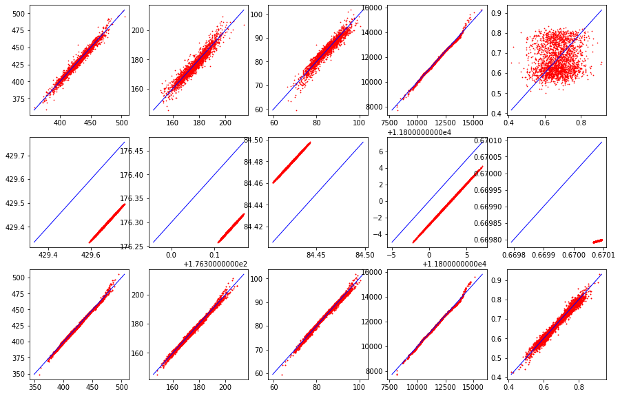
We observe that all the Q-Q plots indicate that the second sample is drawn from a distribution different from the Gaussian distribution with mean and covariance matrix . Notably, the EOT Q-Q plots look very different as compared to the OT and geometric Q-Q plots, possibly due to the regularization parameter not being sufficiently small. Due to computational limitations, we were unable to select smaller than . On the other hand, the OT Q-Q plots more prominently highlight the dissimilarities between the two samples, particularly evident in the -th component (note that the scaling is very different when comparing with other components) of the plots. It is important to note that none of the plots exhibit clear features of the distribution, like heavy tails. Compared to the Q-Q plots conducted after standardizing both samples in Example 6.2 and Section 7.2, this drawback indicates that standardizing the samples when working with real data might be a better approach.