Scalar perturbations from inflation in the presence of gauge fields

Abstract

We study how Abelian-gauge-field production during inflation affects scalar perturbations in the case when the gauge field interacts with the inflaton directly (by means of generic kinetic and axial couplings) and via gravity. The homogeneous background solution is defined by self-consistently taking into account the backreaction of the gauge field on the evolution of the inflaton and the scale factor. For the perturbations on top of this background, all possible scalar contributions coming from the inflaton, the metric, and the gauge field are considered. We derive a second-order differential equation for the curvature perturbation, $\zeta$, capturing the impact of the gauge field, both on the background dynamics and on the evolution of scalar perturbations. The latter is described by a source term in the $\zeta$-equation, which is quadratic in the gauge-field operators and leads to non-Gaussianities in the curvature perturbations. We derive general expressions for the induced scalar power spectrum and bispectrum. Finally, we apply our formalism to the well-known case of axion inflation without backreaction. Numerical results show that, in this example, the effect of including metric perturbations is small for values of the gauge-field production parameter $\xi>3$. This is in agreement with the results of previous studies in the literature. However, in the region of smaller values, $\xi\lesssim 2$, our new results exhibit order-of-unity deviations when compared to previous results.

I Introduction

Inflation is an important pillar of the standard model of cosmology, $\Lambda$CDM. The main role played by this period of very rapid expansion before the hot Big Bang [1, 2, 3, 4, 5, 6] is that it leads to the amplification of vacuum fluctuations of the inflaton field and of the metric [7, 8, 9, 10, 11, 12]. This mechanism for the generation of cosmological perturbations is supported by observations of the cosmic microwave background (CMB) [13, 14, 15] and of the cosmological large scale structure (LSS) [16, 17]; for reviews, see Refs. [18, 19, 20, 21, 22]. In the simplest models of inflation, the scalar fluctuations generated during inflation, which are the seeds of the small density fluctuations in the hot cosmic plasma after inflation, are very close to Gaussian, which is in good agreement with observations [23, 24, 25]. Thus far, no primordial non-Gaussianities (PNG) have been observed, and inflation is characterized purely by the primordial power spectrum of scalar perturbations. Clearly, the detection of PNG would open a new window to study the physics of inflation, making it a vitally important observable. Processes during inflation that may lead to a measurable PNG are, therefore, of great interest.

Another subject of great interest is the origin of magnetic fields in cosmology. Magnetic fields are ubiquitous in the Universe [26, 27, 28, 29] and have been observed in galaxies, even at high redshifts [30], in clusters [31, 32], in filaments [33, 34], and, albeit indirectly through the observation of blazar spectra, even in voids [35, 36, 37, 38, 39, 40, 41, 42, 43, 44, 45, 46] (for a review, see Ref. [47]). In Ref. [48], a lower limit of about $10^{-17}\,$Gauss was derived for the amplitude of large-scale magnetic fields in voids. Such fields are difficult to generate in the late stages of the evolution of the Universe. Therefore, processes in the early Universe leading to the generation of magnetic fields seem more plausible. The authors of Ref. [49] recently argued that blazar observations require the intergalactic magnetic field to fill a fraction $f\gtrsim 0.67$ of space, which again points to a primordial origin, through processes during inflation or cosmological phase transitions.

To generate magnetic fields during inflation, the conformal symmetry of the electromagnetic field has to be broken [50]. This can be done through a coupling of the gauge field to the inflaton, to the Ricci scalar or to the Riemann tensor [51]. During a phase of nearly de Sitter inflation, all these couplings are in fact equivalent. The amplification of gauge-field vacuum fluctuations coupled to the inflaton during inflation has been studied intensively in the past; see the seminal works [51, 52, 53, 54, 55] and the review articles [56, 57, 58, 59, 60]. The homogeneous dynamics of the inflaton leads to the production of gauge fields due to coupling between the fields. On the other hand, these gauge fields, through their interaction with the inflaton and gravity, affect the inflaton and the metric fluctuations. A systematic perturbative study of this effect is the goal of the present paper.

There is a big body of literature in which the production of curvature perturbations in the presence of vector fields during inflation is studied. They consider the kinetic coupling $\propto I(\phi)F_{\mu\nu}F^{\mu\nu}$ [61, 62, 63, 64, 65, 66, 67, 68, 69, 70, 71, 72, 73, 74, 75, 76, 77, 78, 79, 80, 81] or the axial coupling $\propto I(\phi)F_{\mu\nu}\tilde{F}^{\mu\nu}$ [82, 83, 84, 85, 86, 87, 88, 89, 90, 91, 92, 93, 94, 95, 96, 97, 98, 99, 100] of the gauge field to the (pseudo)scalar inflaton or spectator field. In most cases, Abelian gauge fields were studied, except for Refs. [63, 92, 95, 96, 98], which deal with non-Abelian fields. References [101, 102, 103, 104] derive model-independent results for scalar perturbations in the presence of gauge fields. In addition to perturbative studies, numerical simulations on a lattice have been performed in Refs. [105, 106, 107].

In a previous paper [108], some of us found that the interaction of the gauge field with the inflaton leads to considerable backreaction onto the inflaton dynamics, which actually prolongs inflation. This is in agreement with similar analyses [97, 109, 110] and fully numerical studies [107]. For this reason, we expect that the influence of gauge-field perturbations on the scalar perturbations of the metric and the inflaton, which seed the density fluctuations observed in the Universe today, can be considerable. Especially, as we shall see, because these fluctuations are non-Gaussian and may lead to observable PNGs. However, to the best of our knowledge, a self-consistent treatment of the impact of gauge fields on both the background evolution and the scalar perturbations (including those of metric) is still missing in the literature. This provides the main motivation for the present work.

We treat the gauge fields as sources of perturbations in the curvature and neglect the backreaction of metric perturbations on the evolution of the gauge field sources. This formalism has been first used in [111] and later generalized in Ref. [112]. In the present situation, however, the sources also interact with the inflaton field via nongravitational interactions and thus backreact on the evolution of the universe. Therefore, metric perturbations have to be taken into account also in the evolution equations of the source terms. We extend the formalism derived in the above references to take these modifications consistently into account.

The remainder of this paper is organized as follows: In the next section, we present the Lagrangian for the type of models studied in this paper and the resulting equations of motion for all background quantities. In Section III, which is the heart of the present work, we derive the full set of equations describing the evolution of scalar perturbations, taking into account (i) linear perturbations of the inflaton, (ii) scalar linear perturbations of the metric as well as (iii) perturbations up to second order in the gauge field (which are first order perturbations in its energy momentum tensor). We then derive a master equation for the gauge-invariant curvature fluctuation $\zeta$, which accounts for all sources of scalar perturbations in our model, including the contributions from the gauge fields. In Section IV we derive general expressions for the two- and three-point correlation functions of $\zeta$ in Fourier space, i.e., the power spectrum and the bispectrum. We write these in terms of the gauge-field mode functions and the vacuum inflaton perturbations. In Section V, we illustrate our formalism with a simple example and compare our results to the literature. Finally, in Section VI, we conclude and present an outlook on the future applications of our formalism. Some lengthy derivations of important equations and explicit expressions for the constituents of the differential equation for the variable $\zeta$ are deferred to several Appendices.
Notation: We work with a mostly-negative metric signature, $\left(+,-,-,-\right)$, and denote conformal time by $\eta$. A prime on a quantity denotes the derivative of this quantity w.r.t. $\eta$. For functions depending on a different argument, though, a prime denotes a derivative w.r.t. this argument. In these cases, the argument is always shown explicitly. For instance, $V^{\prime}(\phi)$, $I_{1}^{\prime}(\phi)$, and $I_{2}^{\prime}(\phi)$ denote derivatives of theses functions w.r.t. the scalar field $\phi$. The conformal Hubble rate is denoted by $\mathcal{H}=a^{\prime}/a=aH$, where $H$ is the physical Hubble rate. Spacetime indices are denoted by lower-case Greek letters, while spatial indices are lower-case Latin letters. Spatial vectors are written in boldface. The three-dimensional Levi-Civita symbol is denoted by $\varepsilon_{ijk}=\varepsilon^{ijk}$. Throughout the work, we use natural units and set $\hbar=c=1$. We use the notation $M_{\mathrm{P}}=(8\pi G)^{-1/2}\approx 2.43\times 10^{18}\,{\rm GeV}$ for the reduced Planck mass.

II Model and background evolution

We consider a model of inflation with a real scalar inflaton field, $\phi$, and an Abelian gauge field, $A_{\mu}$, which can have both kinetic and axial couplings to the inflaton. Such general model breaks spatial parity $P$ explicitly. The corresponding action has the form:

$$S[g_{\mu\nu},\phi,A_{\mu}] =\!\int\!\!d^{4}x\sqrt{-g}\Big{[}-\frac{M_{\mathrm{P}}^{2}}{2}R+\frac{1}{2}g^{\mu\nu}\partial_{\mu}\phi\partial_{\nu}\phi-V(\phi)-\frac{1}{4}I_{1}(\phi)(\!\!(F_{\mu\nu}F^{\mu\nu})\!\!)-\frac{1}{4}I_{2}(\phi)(\!\!(F_{\mu\nu}\tilde{F}^{\mu\nu})\!\!)\Big{]}\,,$$ (1)

where $g_{\mu\nu}$ is the spacetime metric, $g=\mathrm{det}\,g_{\mu\nu}$ is its determinant, $R$ is the Ricci curvature scalar, $V(\phi)$ is the inflaton potential, $F_{\mu\nu}=\partial_{\mu}A_{\nu}-\partial_{\nu}A_{\mu}$ is the field-strength tensor and $\tilde{F}^{\mu\nu}=1/2\,\epsilon^{\mu\nu\alpha\beta}F_{\alpha\beta}/\sqrt{-g}$ is its dual. Here, $\varepsilon^{\mu\nu\alpha\beta}$ (with $\varepsilon^{0123}=+1$) is the totally antisymmetric Levi-Civita symbol in four dimensions. In the last two terms in the action, we introduced the notation $(\!\!(\dots)\!\!)$ for the symmetrized product of two operators

$$(\!\!(PQ)\!\!)\equiv\frac{1}{2}(PQ+QP)\,,$$

which, after quantisation, may no longer commute. Introduction of this symmetrization is prescribed by the correspondence principle if we write down the action in terms of quantum fields. This symmetrization, although not strictly necessary yet, is introduced here for convenience in deriving later equations like, for example, Eq. (2).

The functions $I_{1,2}(\phi)$ in the action (1) are, respectively, the kinetic and axial couplings of the gauge field to the inflaton. For the sake of generality, we will not specify explicit forms of the inflaton potential and the coupling functions $I_{1,2}(\phi)$. However, in any case, the kinetic coupling function $I_{1}(\phi)$ must be (i) positive in order to ensure the positive definiteness of the gauge-field energy density and (ii) never much smaller than unity during inflation in order to avoid the strong coupling problem. On the other hand, the axial coupling function $I_{2}(\phi)$ is completely arbitrary, because it does not enter the energy–momentum tensor and does not have any impact on the coupling of other matter to the gauge field.

The energy–momentum tensor is obtained by varying the matter part (inflaton and gauge field) of the action (1) w.r.t. the inverse metric $g^{\mu\nu}$,

$$T_{\mu\nu}=\partial_{\mu}\phi\partial_{\nu}\phi-I_{1}(\phi)g^{\alpha\beta}(\!\!(F_{\mu\alpha}F_{\nu\beta})\!\!)-g_{\mu\nu}\left[\frac{1}{2}\partial_{\alpha}\phi\partial^{\alpha}\phi-V(\phi)-\frac{1}{4}I_{1}(\phi)(\!\!(F_{\alpha\beta}F^{\alpha\beta})\!\!)\right]\,.$$ (2)

The Einstein equations read as

$$G_{\mu\nu}=\frac{1}{M_{\mathrm{P}}^{2}}T_{\mu\nu}\,,$$ (3)

where $G_{\mu\nu}$ is the Einstein tensor. The modified Maxwell equations are obtained by varying the action (1) w.r.t. the gauge field $A_{\mu}$,

$$\frac{1}{\sqrt{-g}}\partial_{\mu}\left[\sqrt{-g}I_{1}(\phi)F^{\mu\nu}\right]=-\tilde{F}^{\mu\nu}\partial_{\mu}I_{2}(\phi)\,.$$ (4)

They are supplemented by the Bianchi identities

$$\frac{1}{\sqrt{-g}}\partial_{\mu}\left[\sqrt{-g}\tilde{F}^{\mu\nu}\right]=0\,.$$ (5)

Finally, varying the action (1) w.r.t. the inflaton field, we obtain the inflaton equation of motion,

$$\frac{1}{\sqrt{-g}}\partial_{\mu}\left[\sqrt{-g}g^{\mu\nu}\partial_{\nu}\phi\right]+V^{\prime}(\phi)=-\frac{1}{4}I^{\prime}_{1}(\phi)(\!\!(F_{\mu\nu}F^{\mu\nu})\!\!)-\frac{1}{4}I^{\prime}_{2}(\phi)(\!\!(F_{\mu\nu}\tilde{F}^{\mu\nu})\!\!)\,.$$ (6)

Let us first describe the solutions to these equations in the case of a spatially flat, homogeneous and isotropic Friedmann–Lemaître–Robertson–Walker (FLRW) geometry. The corresponding metric is given by

$$g^{(0)}_{\mu\nu}dx^{\mu}dx^{\nu}=a^{2}(\eta)[d\eta^{2}-\delta_{ij}dx^{i}dx^{j}]\,,$$ (7)

where $a(\eta)$ is the scale factor. The background inflaton field, which is considered as a spatially homogeneous classical field, is denoted by $\phi_{c}\left(\eta\right)=\left<\phi\left(\eta,\bm{x}\right)\right>$. We define the electric- and magnetic-field three-vectors from the components of the field-strength tensor,

$$F_{0i}=a^{2}E^{i}\,,\quad F_{ij}=-a^{2}\varepsilon_{ijk}B^{k}\,.$$ (8)

These correspond to the electric and magnetic fields as measured by a comoving observer in a background FLRW universe.

In this case, the Einstein equations simply become the Friedmann equations, which, for our matter content, read

$$\frac{a^{\prime 2}}{a^{2}}\equiv\mathcal{H}^{2} =\frac{1}{3M_{\mathrm{P}}^{2}}\bigg{\{}\frac{\phi_{c}^{\prime 2}}{2}+a^{2}V(\phi_{c})+\frac{a^{2}}{2}I_{1}(\phi_{c})\Big{[}\langle\bm{E}^{2}\rangle+\langle\bm{B}^{2}\rangle\Big{]}\bigg{\}}\,,$$ (9)

$$2\mathcal{H}^{\prime}+\mathcal{H}^{2} =-\frac{1}{M_{\mathrm{P}}^{2}}\bigg{\{}\frac{\phi_{c}^{\prime 2}}{2}-a^{2}V(\phi_{c})+\frac{a^{2}}{6}I_{1}(\phi_{c})\Big{[}\langle\bm{E}^{2}\rangle+\langle\bm{B}^{2}\rangle\Big{]}\bigg{\}}\,.$$ (10)

Here, $\langle\bm{E}^{2}\rangle$ and $\langle\bm{B}^{2}\rangle$ are the vacuum expectation values of the gauge-field contributions to the total energy density and pressure.

The Klein–Gordon equation for the scalar field in this background becomes

$$\phi^{\prime\prime}_{c}+2\mathcal{H}\phi^{\prime}_{c}+a^{2}V^{\prime}(\phi_{c})=\frac{1}{2}a^{2}I^{\prime}_{1}(\phi_{c})\Big{[}\langle\bm{E}^{2}\rangle-\langle\bm{B}^{2}\rangle\Big{]}+a^{2}I^{\prime}_{2}(\phi_{c})\langle(\!\!(\bm{E}\cdot\bm{B})\!\!)\rangle\,.$$ (11)

Note that we apply the symmetrization operation explicitly only for the products of the electric and magnetic fields, $(\!\!(E_{j}B_{k})\!\!)$, as the corresponding field operators do not commute, see Refs. [113, 114, 115, 116]. In cases where the operators obviously commute, e.g., for $\bm{E}^{2}$, this operation is omitted for the sake of brevity.

The Maxwell equations read as

$$\operatorname{div}\bm{B} =0\,,$$ (12)

$${\bm{B}}^{\prime}+2\mathcal{H}\bm{B}+\operatorname{rot}\bm{E} =0\,,$$ (13)

$$\operatorname{div}\bm{E} =0\,,$$ (14)

$$\bm{E}^{\prime}+2\mathcal{H}\bm{E}-\operatorname{rot}\bm{B}+\frac{I^{\prime}_{1}(\phi_{c})}{I_{1}(\phi_{c})}\phi^{\prime}_{c}\bm{E}+\frac{I^{\prime}_{2}(\phi_{c})}{I_{1}(\phi_{c})}\phi^{\prime}_{c}\bm{B} =0\,.$$ (15)

With these, we can derive equations for the time derivatives of the vacuum expectation values to which only the background quantities contribute:

$$\langle\bm{E}^{2}\rangle^{\prime} =-\left[4\mathcal{H}+2\frac{I^{\prime}_{1}(\phi_{c})}{I_{1}(\phi_{c})}\phi^{\prime}_{c}\right]\langle\bm{E}^{2}\rangle-2\frac{I^{\prime}_{2}(\phi_{c})}{I_{1}(\phi_{c})}\phi^{\prime}_{c}\langle(\!\!(\bm{E}\cdot\bm{B})\!\!)\rangle+2\langle(\!\!(\bm{E}\cdot\operatorname{rot}\bm{B})\!\!)\rangle\,,$$ (16)

$$\langle\bm{B}^{2}\rangle^{\prime} =-4\mathcal{H}\langle\bm{B}^{2}\rangle-2\langle(\!\!(\bm{E}\cdot\operatorname{rot}\bm{B})\!\!)\rangle\,,$$ (17)

$$\langle(\!\!(\bm{E}\cdot\bm{B})\!\!)\rangle^{\prime} =-\left[4\mathcal{H}+\frac{I^{\prime}_{1}(\phi_{c})}{I_{1}(\phi_{c})}\phi^{\prime}_{c}\right]\langle(\!\!(\bm{E}\cdot\bm{B})\!\!)\rangle-\frac{I^{\prime}_{2}(\phi_{c})}{I_{1}(\phi_{c})}\phi^{\prime}_{c}\langle\bm{B}^{2}\rangle-\langle\bm{E}\cdot\operatorname{rot}\bm{E}\rangle+\langle\bm{B}\cdot\operatorname{rot}\bm{B}\rangle\,.$$ (18)

These equations for the expectation values are not closed as new terms with a larger number of spatial curls appear on their right-hand side. Writing down equations of motion for those new terms leads to an infinite chain of differential equations. However, there is a way to truncate this system at a certain finite order, which allows to solve it numerically. This method, known as the gradient-expansion formalism, was developed in Refs. [117, 118, 109, 108] and can be used to obtain the background solution in the presence of gauge-field backreaction.

III Scalar perturbations

We now switch to a perturbed FLRW universe with spatially flat sections. We consider only scalar perturbations and will work in the longitudinal gauge. However, our final master equation will be gauge-invariant. Of course, gauge fields also generate vector and tensor fluctuations; but we do not study these here.

The situation we have in mind is a phase of slow roll of the scalar field with its energy density dominated by the scalar-field potential leading to nearly de Sitter expansion. The slow roll parameters

$$\epsilon=-\frac{\dot{H}}{H^{2}}\,,\qquad\eta_{V}=\left|\frac{\ddot{\phi}_{c}}{H\dot{\phi}_{c}}\right|$$ (19)

are assumed to be much smaller than unity. An overdot is a derivative w.r.t. cosmic time $t$.

At early times, subhorizon modes with $|k\eta|\gg 1$ (where $k=|\bm{k}|$ is the absolute value of the comoving momentum $\bm{k}$ carried by the perturbation mode) are in the vacuum state. Scalar-field perturbations are then excited by the rapid expansion, while gauge modes are excited due to their coupling to the background inflaton field. How this happens in detail is governed by the perturbation equations that we derive in this section. The quantum vacuum simply determines the initial state for each mode.

The metric is given by

$$g_{\mu\nu}dx^{\mu}dx^{\nu} =(1+2\Psi)a^{2}d\eta^{2}-(1-2\Phi)a^{2}\delta_{ij}dx^{i}dx^{j}\,,$$ (20)

where $\Psi(\eta,\bm{x})$ and $\Phi(\eta,\bm{x})$ are the Bardeen potentials describing small perturbations of the metric, $|\Phi|,\,|\Psi|\ll 1$. The square root of the determinant of the metric up to linear order in the Bardeen potentials reads $\sqrt{-g}\approx a^{4}(1+\Psi-3\Phi)$.

The definitions of the electric- and magnetic-field three-vectors remain unchanged and are given by Eq. (8). The contravariant components of the field-strength tensor and the components of the dual tensor can be expressed in terms of $\bm{E}$, $\bm{B}$ and the metric perturbations, given by Eqs. (124)–(129). While we work to first order in the metric perturbations in these expressions, we have not made any assumptions about the magnitude of the gauge-field amplitude so far.

In addition to the Bardeen potentials, we define the following perturbation variables:

$$\delta\varphi(\eta,\,\bm{x})\equiv\phi(\eta,\,\bm{x})-\phi_{c}(\eta)$$ (21)

for the inflaton perturbation and

$$\delta_{P_{i}Q_{j}}=(\!\!(P_{i}Q_{j})\!\!)-\frac{1}{3}\delta_{ij}\langle(\!\!(\bm{P}\cdot\bm{Q})\!\!)\rangle$$ (22)

for the product of any two gauge-field vector quantities, where $\bm{P}$ and $\bm{Q}$ can each be equal to any spatial vectors out of the set $\{\bm{E}$, $\bm{B}$, $\operatorname{rot}\bm{E}$, $\operatorname{rot}\bm{B},\operatorname{rot}^{2}\bm{E},\dots\}$. Here, again, $\langle\ldots\rangle$ denotes the vacuum expectation value which, as a consequence of the isotropy of the background, is independent of position. In all equations of motion, only the terms up to linear order in these perturbations are retained.

It may appear confusing that we consider terms only to the first order in the inflaton perturbations but to the second order in the gauge fields. However, this is necessary if we want to study the backreaction of the gauge fields onto the inflaton perturbations. As we shall see, only the perturbation variables defined above enter in the inflaton-perturbation equations. To determine the gauge fields generated during inflation, we will, however, have to solve Eqs. (4) and (5), which are linear in the gauge fields.

III.1 Perturbed Einstein equations

In Appendix A, we explicitly write down the perturbed Einstein and energy–momentum tensors. While the contributions from inflaton perturbations are always scalar, this is not the case for the gauge field. In order to isolate the scalar perturbations from the gauge-field energy–momentum tensor, we introduce the following set of sources:

$$F_{\rho} =\frac{a^{2}}{2M_{\mathrm{P}}^{2}}\delta T^{\ 0\,\mathrm{(EM)}}_{0}=\frac{a^{2}I_{1}(\phi_{c})}{4M_{\mathrm{P}}^{2}}\Big{[}\delta_{\bm{E}^{2}}+\delta_{\bm{B}^{2}}\Big{]}\,,$$ (23)

$$F_{v} =\frac{a^{2}}{2M_{\mathrm{P}}^{2}}\frac{\partial_{i}}{\triangle}\delta T^{\ 0\,\mathrm{(EM)}}_{i}=-\frac{a^{2}I_{1}(\phi_{c})}{2M_{\mathrm{P}}^{2}}\frac{\partial_{i}}{\triangle}\varepsilon_{ijk}\delta_{E_{j}B_{k}}\,,$$ (24)

$$F_{p} =-\frac{a^{2}}{2M_{\mathrm{P}}^{2}}\frac{1}{3}\delta^{i}_{j}\ \delta T^{\ j\,\mathrm{(EM)}}_{i}=\frac{a^{2}I_{1}(\phi_{c})}{12M_{\mathrm{P}}^{2}}\Big{[}\delta_{\bm{E}^{2}}+\delta_{\bm{B}^{2}}\Big{]}=\frac{1}{3}F_{\rho}\,,$$ (25)

$$F_{\pi} =-\frac{a^{2}}{2M_{\mathrm{P}}^{2}}\frac{3}{2\triangle^{2}}\Big{(}\partial_{i}\partial_{j}-\frac{1}{3}\delta^{i}_{j}\triangle\Big{)}\delta T^{\ j\,\mathrm{(EM)}}_{i}$$

$$=-\frac{3a^{2}I_{1}(\phi_{c})}{4M_{\mathrm{P}}^{2}}\frac{\partial_{i}\partial_{j}}{\triangle^{2}}\left[\delta_{E_{i}E_{j}}+\delta_{B_{i}B_{j}}\right]+\frac{a^{2}I_{1}(\phi_{c})}{4M_{\mathrm{P}}^{2}}\frac{1}{\triangle}\left[\delta_{\bm{E}^{2}}+\delta_{\bm{B}^{2}}\right]\,.$$ (26)

Here, all spatial indices $i,j,k$ are raised and lowered by the Euclidean metric. Triangle $\triangle$ denotes the spatial Laplacian operator. The inverse Laplacian operators are easily interpreted in Fourier space. Their appearance explicitly shows that the decomposition into scalar, vector and tensor contributions is nonlocal.

With these definitions, the first-order perturbed Einstein equations become

$$\triangle\Phi-3\mathcal{H}\Phi^{\prime}-3\mathcal{H}^{2}\Psi= \frac{a^{2}}{2M_{\mathrm{P}}^{2}}\bigg{\{}\frac{\phi^{\prime}_{c}}{a^{2}}\delta\varphi^{\prime}+\Big{[}V^{\prime}(\phi_{c})\!+\!\frac{1}{2}I^{\prime}_{1}(\phi_{c})\Big{(}\langle\bm{E}^{2}\rangle\!+\!\langle\bm{B}^{2}\rangle\Big{)}\Big{]}\delta\varphi$$

$$-\frac{\phi^{\prime 2}_{c}}{a^{2}}\Psi+I_{1}(\phi_{c})\Big{[}(\Phi-\Psi)\langle\bm{E}^{2}\rangle+2\Phi\langle\bm{B}^{2}\rangle\Big{]}\bigg{\}}+F_{\rho}\,,$$ (27)

$$\Phi^{\prime}+\mathcal{H}\Psi= \frac{\phi^{\prime}_{c}}{2M_{\mathrm{P}}^{2}}\delta\varphi+F_{v}\,,$$ (28)

$$\Phi^{\prime\prime}+\mathcal{H}(\Psi^{\prime}+2\Phi^{\prime})+(2\mathcal{H}^{\prime}+\mathcal{H}^{2})\Psi= \frac{a^{2}}{2M_{\mathrm{P}}^{2}}\bigg{\{}\frac{\phi^{\prime}_{c}}{a^{2}}\delta\varphi^{\prime}-\Big{[}V^{\prime}(\phi_{c})\!-\!\frac{1}{6}I^{\prime}_{1}(\phi_{c})\Big{(}\langle\bm{E}^{2}\rangle\!+\!\langle\bm{B}^{2}\rangle\Big{)}\Big{]}\delta\varphi$$

$$-\frac{\phi^{\prime 2}_{c}}{a^{2}}\Psi+\frac{1}{3}I_{1}(\phi_{c})\Big{[}(\Phi-\Psi)\langle\bm{E}^{2}\rangle+2\Phi\langle\bm{B}^{2}\rangle\Big{]}\bigg{\}}+\frac{1}{3}(F_{\rho}+2\triangle F_{\pi})\,,$$ (29)

$$\Phi-\Psi= 2F_{\pi}\,.$$ (30)

The first two equations are the $00$ and $0i$ constraint equations while the last two are the $ii$ and $i\neq j$ evolution equations. The gauge field enters here in two ways. Firstly, through their coupling to the inflaton field, the background terms $\langle\bm{B}^{2}\rangle$ and $\langle\bm{E}^{2}\rangle$ couple to $\delta\varphi$. Secondly, the energy–momentum tensor generates metric perturbations via the functions $F_{\rho}$, $F_{v}$, and $F_{\pi}$.

Using Eq. (28), we can rewrite Eq. (27) in a simpler form

$$\triangle\Phi= \frac{a^{2}}{2M_{\mathrm{P}}^{2}}\bigg{\{}\frac{\phi^{\prime}_{c}}{a^{2}}(\delta\varphi^{\prime}+3\mathcal{H}\delta\varphi)+\Big{[}V^{\prime}(\phi_{c})+\frac{1}{2}I^{\prime}_{1}(\phi_{c})\Big{(}\langle\bm{E}^{2}\rangle+\langle\bm{B}^{2}\rangle\Big{)}\Big{]}\delta\varphi$$

$$-\frac{\phi^{\prime 2}_{c}}{a^{2}}\Psi+I_{1}(\phi_{c})\Big{[}(\Phi-\Psi)\langle\bm{E}^{2}\rangle+2\Phi\langle\bm{B}^{2}\rangle\Big{]}\bigg{\}}+F_{\rho}+3\mathcal{H}F_{v}\,.$$ (31)

With the help of Eq. (30), $\Psi$ can be replaced by $\Phi$, and, with Eq. (28), $\delta\varphi$ can be eliminated. One thus obtains an equation for $\Phi$ alone, which, however, contains not only the source terms $F_{\alpha}$ but also their time derivatives. Since we prefer to work with the curvature perturbation variable $\zeta$, we do not write the resulting equation here.

III.2 Maxwell’s equations and source terms

In order to determine the source terms $F_{\alpha}$ and their time derivatives, $F^{\prime}_{\alpha}$, we must solve the Maxwell equations. Accounting for the scalar metric and inflaton perturbations in Maxwell’s equations yields

$$\operatorname{div}\bm{B} =0\,,$$ (32)

$$\bm{B}^{\prime}+2\mathcal{H}\bm{B}+\operatorname{rot}\bm{E} =0\,,$$ (33)

$$\operatorname{div}\bm{E}+\Big{[}\frac{I^{\prime}_{1}(\phi_{c})}{I_{1}(\phi_{c})}\bm{E}+\frac{I^{\prime}_{2}(\phi_{c})}{I_{1}(\phi_{c})}\bm{B}\Big{]}\cdot\bm{\nabla}\delta\varphi-\bm{E}\cdot\bm{\nabla}(\Phi+\Psi) =0\,,$$ (34)

$$\bm{E}^{\prime}+2\mathcal{H}\bm{E}-\operatorname{rot}\bm{B}+\Big{[}\frac{I^{\prime}_{1}(\phi_{c})}{I_{1}(\phi_{c})}\bm{E}+\frac{I^{\prime}_{2}(\phi_{c})}{I_{1}(\phi_{c})}\bm{B}\Big{]}(\phi^{\prime}_{c}+\delta\varphi^{\prime})+\Big{[}\Big{(}\frac{I^{\prime}_{1}(\phi_{c})}{I_{1}(\phi_{c})}\bm{B}-\frac{I^{\prime}_{2}(\phi_{c})}{I_{1}(\phi_{c})}\bm{E}\Big{)}\!\times\!\bm{\nabla}\delta\varphi\Big{]}$$

$$+\bigg{[}\Big{(}\frac{I^{\prime\prime}_{1}(\phi_{c})}{I_{1}(\phi_{c})}-\frac{I^{\prime}_{1}(\phi_{c})^{2}}{I_{1}(\phi_{c})^{2}}\Big{)}\bm{E}+\Big{(}\frac{I^{\prime\prime}_{2}(\phi_{c})}{I_{1}(\phi_{c})}-\frac{I^{\prime}_{1}(\phi_{c})I^{\prime}_{2}(\phi_{c})}{I_{1}(\phi_{c})^{2}}\Big{)}\bm{B}\bigg{]}\phi^{\prime}_{c}\delta\varphi$$

$$-(\Phi+\Psi)^{\prime}\bm{E}-2(\Phi+\Psi)\operatorname{rot}\bm{B}+[\bm{B}\!\times\!\bm{\nabla}(\Phi+\Psi)]+\frac{I^{\prime}_{2}(\phi_{c})}{I_{1}(\phi_{c})}\phi^{\prime}_{c}(\Phi+\Psi)\bm{B} =0\,.$$ (35)

With the help of the perturbed Maxwell equations, (32) to (35), we determine the time derivatives of the source terms:

$$F^{\prime}_{\rho}= \Big{[}-2\mathcal{H}+\frac{I^{\prime}_{1}(\phi_{c})}{I_{1}(\phi_{c})}\phi^{\prime}_{c}\Big{]}F_{\rho}+\triangle F_{v}-\frac{a^{2}\phi^{\prime}_{c}}{2M_{\mathrm{P}}^{2}}[I^{\prime}_{1}(\phi_{c})\delta_{\bm{E}^{2}}+I^{\prime}_{2}(\phi_{c})\delta_{\bm{E}\cdot\bm{B}}]$$

$$-\frac{a^{2}I_{1}(\phi_{c})}{2M_{\mathrm{P}}^{2}}\bigg{\{}\langle\bm{E}^{2}\rangle\Big{[}\frac{I^{\prime}_{1}(\phi_{c})}{I_{1}(\phi_{c})}\delta\varphi^{\prime}+\Big{(}\frac{I^{\prime\prime}_{1}(\phi_{c})}{I_{1}(\phi_{c})}-\frac{I^{\prime 2}_{1}(\phi_{c})}{I^{2}_{1}(\phi_{c})}\Big{)}\phi^{\prime}_{c}\delta\varphi-(\Phi+\Psi)^{\prime}\Big{]}$$

$$+\langle(\!\!(\bm{E}\cdot\bm{B})\!\!)\rangle\Big{[}\frac{I^{\prime}_{2}(\phi_{c})}{I_{1}(\phi_{c})}\delta\varphi^{\prime}+\Big{(}\frac{I^{\prime\prime}_{2}(\phi_{c})}{I_{1}(\phi_{c})}-\frac{I^{\prime}_{1}(\phi_{c})I^{\prime}_{2}(\phi_{c})}{I^{2}_{1}(\phi_{c})}\Big{)}\phi^{\prime}_{c}\delta\varphi+\frac{I^{\prime}_{2}(\phi_{c})}{I_{1}(\phi_{c})}\phi^{\prime}_{c}(\Phi+\Psi)\Big{]}$$

$$+2\langle(\!\!(\bm{E}\cdot\operatorname{rot}\bm{B})\!\!)\rangle(\Phi+\Psi)\bigg{\}}\,,$$ (36)

$$F^{\prime}_{v}= -2\mathcal{H}F_{v}+\frac{2}{3}\triangle F_{\pi}+\frac{1}{3}F_{\rho}-\frac{a^{2}}{2M_{\mathrm{P}}^{2}}\bigg{\{}\frac{1}{3}\langle\bm{E}^{2}\rangle\big{[}I^{\prime}_{1}(\phi_{c})\delta\varphi-I_{1}(\phi_{c})(\Phi+\Psi)\big{]}+\langle(\!\!(\bm{E}\cdot\bm{B})\!\!)\rangle I^{\prime}_{2}(\phi_{c})\delta\varphi$$

$$-\frac{2}{3}\langle\bm{B}^{2}\rangle\big{[}I^{\prime}_{1}(\phi_{c})\delta\varphi+I_{1}(\phi_{c})(\Phi+\Psi)\big{]}\bigg{\}}\,,$$ (37)

$$F^{\prime}_{\pi}= \Big{[}-2\mathcal{H}+\frac{I^{\prime}_{1}(\phi_{c})}{I_{1}(\phi_{c})}\phi^{\prime}_{c}\Big{]}F_{\pi}$$

$$-\frac{a^{2}I_{1}(\phi_{c})}{2M_{\mathrm{P}}^{2}}\Big{(}\frac{\delta_{ij}}{\triangle}-3\frac{\partial_{i}\partial_{j}}{\triangle^{2}}\Big{)}\Big{[}\frac{I^{\prime}_{1}(\phi_{c})}{I_{1}(\phi_{c})}\phi^{\prime}_{c}\delta_{E_{i}E_{j}}+\frac{I^{\prime}_{2}(\phi_{c})}{I_{1}(\phi_{c})}\phi^{\prime}_{c}\delta_{E_{i}B_{j}}+\delta_{(\operatorname{rot}\bm{E})_{i}B_{j}}-\delta_{(\operatorname{rot}\bm{B})_{i}E_{j}}\Big{]}\,.$$ (38)

Note that the equations of motion for $F_{\rho}$ and $F_{v}$ contain metric perturbations while the one for $F_{\pi}$ does not. This fact will be important below, where we derive a differential equation for the curvature-perturbation variable $\zeta$.

III.3 Perturbed Klein–Gordon equation

For completeness, we also write down the perturbed Klein–Gordon equation, which can be directly obtained from Eq. (6) or by combining the Einstein equations:

$$\delta\varphi^{\prime\prime}+2\mathcal{H}\delta\varphi^{\prime}-\triangle\delta\varphi+a^{2} \Big{[}V^{\prime\prime}(\phi_{c})-\frac{I^{\prime\prime}_{1}(\phi_{c})}{2}\Big{(}\langle\bm{E}^{2}\rangle-\langle\bm{B}^{2}\rangle\Big{)}-I^{\prime\prime}_{2}(\phi_{c})\langle(\!\!(\bm{E}\cdot\bm{B})\!\!)\rangle\Big{]}\delta\varphi$$

$$=\, \phi^{\prime}_{c}(\Psi^{\prime}+3\Phi^{\prime})+2(\phi^{\prime\prime}_{c}+2\mathcal{H}\phi^{\prime}_{c})\Psi+a^{2}I^{\prime}_{1}(\phi_{c})\Big{[}(\Phi-\Psi)\langle\bm{E}^{2}\rangle-2\Phi\langle\bm{B}^{2}\rangle\Big{]}$$

$$+a^{2}I^{\prime}_{2}(\phi_{c})\langle(\!\!(\bm{E}\cdot\bm{B})\!\!)\rangle(3\Phi-\Psi)+\frac{a^{2}I^{\prime}_{1}(\phi_{c})}{2}\Big{[}\delta_{\bm{E}^{2}}-\delta_{\bm{B}^{2}}\Big{]}+a^{2}I^{\prime}_{2}(\phi_{c})\delta_{\bm{E}\cdot\bm{B}}\,.$$ (39)

Note that this equation is not independent from the Einstein equations (27)–(28). We will use them interchangeably in our computations below.

III.4 Curvature perturbation variable $\zeta$

The curvature-perturbation variable, $\zeta$, can be expressed in terms of the Bardeen variables as [21]

$$\zeta =\Phi+\frac{\mathcal{H}}{\mathcal{H}^{2}-\mathcal{H}^{\prime}}(\Phi^{\prime}+\mathcal{H}\Psi)$$ (40)

$$=\Phi+\frac{\mathcal{H}}{\mathcal{H}^{2}-\mathcal{H}^{\prime}}\Big{(}\frac{\phi^{\prime}_{c}}{2M_{\mathrm{P}}^{2}}\delta\varphi+F_{v}\Big{)}\,,$$ (41)

where we used Eq. (28) for the second equality. In the absence of gauge fields on the hypersurfaces $\delta\varphi=0$ (unitary gauge), this variable describes the curvature of the spatial sections. It is very useful as it is simply related to the canonical perturbation variable which has to be quantized in order to find the scalar perturbations of the inflaton. In the absence of gauge fields, the scalar perturbations of the metric and the inflaton combine to one degree of freedom which is traditionally cast in terms of this $\zeta$-variable. The advantage of $\zeta$ is that it is constant on large, superhorizon scales in the absence of gauge fields. Therefore, the transition from inflation to the radiation-dominated era, at a time when all relevant modes are superhorizon, is especially simple in terms of this variable. Even though these nice properties are in general lost when gauge fields are present, and despite its rather contrived derivation, we nonetheless aim to find a second-order differential equation for $\zeta$ alone in which the source terms, $F_{\alpha}$, appear on the right-hand side. Standard inflationary predictions are then easily obtained by just setting the right-hand side to zero. This will also allow us to split $\zeta$ into a homogeneous solution, describing the inflaton perturbations, and a peculiar solution, due to the gauge-field source terms.

The derivation of this differential equation for the $\zeta$ variable is presented in full detail in Appendix B. It can be summarized as follows: we use Eqs. (30) and (III.1) to express $\delta\varphi^{\prime}$ as a function of $\Phi$, $\delta\varphi$, and the sources $F_{v}$, $F_{\rho}$, $F_{\pi}$. Then, we write $\Phi^{\prime}$ in terms of $\Phi$, $\delta\varphi$, and the sources with the help of Eqs. (28) and (30). Using Eqs. (29) and (30), we can now find $(\Phi^{\prime}+\mathcal{H}\Psi)^{\prime}$ as a function of $\Phi$, $\delta\varphi$, and the sources. Taking the time derivative of Eq. (41), we can also express $\zeta^{\prime}$ as a function of $\Phi$, $\delta\varphi$, and the sources. We then invert the relations $\zeta=\zeta(\Phi,\,\delta\varphi,\ F_{\alpha})$ and $\zeta^{\prime}=\zeta^{\prime}(\Phi,\,\delta\varphi,\ F_{\alpha})$ to determine $\Phi=\Phi(\zeta,\,\zeta^{\prime},\,F_{\alpha})$ and $\delta\varphi=\delta\varphi(\zeta,\,\zeta^{\prime},\,F_{\alpha})$. Next, we take the time derivative of $\zeta^{\prime}$ and express it as a function of $\Phi$, $\delta\varphi$, the sources and their first time derivatives. Finally, we use the equations of motion for the sources derived in the previous section in order to express $\zeta^{\prime\prime}$ as a function of $\zeta^{\prime}$, $\zeta$, the sources and $F_{\pi}^{\prime}$. This results in the desired second-order differential equation for $\zeta$. This derivation is best performed in Fourier space, where Laplacians simply generate a factor $-k^{2}$. The final equation takes the form:

$$\zeta^{\prime\prime}+p\zeta^{\prime}+q\zeta=r^{(v)}F_{v}+r^{(\rho)}F_{\rho}+r^{(\pi)}_{1}F_{\pi}+r^{(\pi)}_{2}F^{\prime}_{\pi}+r^{(\bm{E}^{2})}\delta_{\bm{E}^{2}}+r^{(\bm{E}\cdot\bm{B})}\delta_{\bm{E}\cdot\bm{B}}\,.$$ (42)

The coefficients $p$, $q$ and $r^{(\alpha)}$ are functions of time which depend only on the background evolution, including the zero-modes, $\langle\bm{E}^{2}\rangle$, $\langle\bm{B}^{2}\rangle$ and $\langle(\!\!(\bm{E}\cdot\bm{B})\!\!)\rangle$. They are determined and presented in detail in Appendix B. We emphasize that the decomposition of the source on the right-hand side of Eq. (42) into six terms is performed merely for convenience. These terms are not independent, but rather depend on the same gauge-field mode functions.

In the case where we may neglect backreaction and set $\langle\bm{E}^{2}\rangle=\langle\bm{B}^{2}\rangle=\langle(\!\!(\bm{E}\cdot\bm{B})\!\!)\rangle=0$, it is easy to check that the coefficients $p$ and $q$ reduce to the usual form,

$$q =k^{2}\,,$$ (43)

$$p =2\frac{\mathcal{H}^{2}-\mathcal{H}^{\prime}}{\mathcal{H}}+\frac{\left(\mathcal{H}^{2}-\mathcal{H}^{\prime}\right)^{\prime}}{\mathcal{H}^{2}-\mathcal{H}^{\prime}}=2\frac{z^{\prime}}{z}\,,$$ (44)

where $$z$$ is the Mukhanov–Sasaki variable,

$$z =\frac{a\,M_{\mathrm{P}}\sqrt{2(\mathcal{H}^{2}-\mathcal{H}^{\prime})}}{\mathcal{H}}=\frac{a\phi_{c}^{\prime}}{\mathcal{H}}\,.$$ (45)

As we have seen in our previous work [108], while the contribution of the gauge fields to the energy momentum tensor remains small, they do significantly affect the inflaton evolution. Therefore, terms like $I^{\prime}_{1}(\phi_{c})\langle\bm{E}^{2}\rangle$ or $I^{\prime}_{2}(\phi_{c})\langle(\!\!(\bm{E}\cdot\bm{B})\!\!)\rangle$ cannot be neglected when compared to $\mathcal{H}\phi_{c}^{\prime}$ or $V^{\prime}$. These are exactly the kind of correction terms which enter $p$ and $q$; see Appendix B for details.

In general, one should treat the scalar variable $\zeta$ on the same footing as the gauge-field sources. For this, one would need to consider a coupled system of equations consisting of Eq. (42), the equations of motion for the sources, Eqs. (36)–(38) for $F_{\rho}$, $F_{v}$, and $F_{\pi}$, and analogous equations for the other source terms. Then, this system of equations would have to be solved with the appropriate initial conditions in a similar way as it is done for the adiabatic and entropy perturbations in multi-field inflationary models; see, e.g., Refs. [119, 120, 121]. This would allow one to take into account the impact of scalar inflaton and metric perturbations on the gauge-field modes. However, we expect this effect to be small compared to the mode amplification which comes from the background evolution via the kinetic and/or axial couplings. Therefore, in what follows, we compute the sources using the gauge-field mode functions determined on a spatially homogeneous background. Hence, we assume in Eq. (42) that the sources on the right-hand side are known as soon as the background solution of the system is obtained.

In order to solve this inhomogeneous equation, we first have to determine its homogeneous solutions, $\zeta_{1}$ and $\zeta_{2}$, which obey

$$\zeta_{1,2}^{\prime\prime}+p\zeta_{1,2}^{\prime}+q\zeta_{1,2}\equiv\mathcal{D}\zeta=0\,.$$ (46)

The Green’s function is then given by

$$G_{\bm{k}}(\eta,\eta^{\prime})=\frac{-\zeta_{1}(\bm{k},\eta)\zeta_{2}(\bm{k},\eta^{\prime})+\zeta_{2}(\bm{k},\eta)\zeta_{1}(\bm{k},\eta^{\prime})}{W(\bm{k},\eta^{\prime})}\theta(\eta-\eta^{\prime})\,,$$ (47)

where $W$ is the Wronskian of the solutions $(\zeta_{1},\leavevmode\nobreak\ \zeta_{2})$,

$$W(\bm{k},\eta^{\prime})=\zeta_{1}(\bm{k},\eta^{\prime})\zeta^{\prime}_{2}(\bm{k},\eta^{\prime})-\zeta_{2}(\bm{k},\eta^{\prime})\zeta^{\prime}_{1}(\bm{k},\eta^{\prime})\,.$$ (48)

It is straightforward to check that the Green’s function (47) satisfies

$$\mathcal{D}G_{\bm{k}}(\eta,\eta^{\prime})=\delta(\eta-\eta^{\prime})$$ (49)

together with the boundary conditions

$$G_{\bm{k}}(\eta,\eta^{\prime}\geq\eta)\equiv 0\,,\quad\frac{\partial}{\partial\eta}G_{\bm{k}}(\eta,\eta^{\prime})\Big{|}_{\eta^{\prime}\to\eta}=1\,,$$ (50)

corresponding to the retarded Green’s function. Then, a particular solution of (42), with the source term $\mathcal{S}_{\bm{k}}(\eta)$ given by the right-hand side of (42), can be written as

$$\zeta_{p}(\bm{k},\eta)=\int\limits_{-\infty}^{\eta}d\eta^{\prime}\,G_{\bm{k}}(\eta,\eta^{\prime})\mathcal{S}_{\bm{k}}(\eta^{\prime})\,.$$ (51)

The general solution of the equation (42) is the sum of a homogeneous- and this particular solution and has the form

$$\zeta_{\bm{k}}(\eta)=\zeta^{(0)}_{\bm{k}}(\eta)+\int\limits_{-\infty}^{\eta}d\eta^{\prime}\,G_{\bm{k}}(\eta,\eta^{\prime})\mathcal{S}_{\bm{k}}(\eta^{\prime})\,.$$ (52)

In general, $\zeta^{(0)}_{\bm{k}}$ is an arbitrary linear combination of $\zeta_{1}$ and $\zeta_{2}$. In our situation, the coefficients have to be chosen such that the homogeneous solution corresponds to the vacuum fluctuations of the canonical variable $v=z\zeta$ on subhorizon scales, $|k\eta|\gg 1$.

IV Two-point and three-point correlation functions

The two contributions in Eq. (52) are statistically independent since the first one can be interpreted as the vacuum fluctuations of the inflaton and the metric scalar degrees of freedom, i.e., the standard inflationary scalar perturbation, while the second one is induced by the gauge-field source $\mathcal{S}$. In practice, this means that there are no correlations between the two terms,

$$\langle\zeta_{\bm{k}}(\eta)\zeta_{\bm{k}^{\prime}}(\eta)\rangle=\langle\zeta^{(0)}_{\bm{k}}(\eta)\zeta^{(0)}_{\bm{k}^{\prime}}(\eta)\rangle+\int\limits_{-\infty}^{\eta}d\eta^{\prime}\int\limits_{-\infty}^{\eta}d\eta^{\prime\prime}\,G_{\bm{k}}(\eta,\eta^{\prime})G_{\bm{k}^{\prime}}(\eta,\eta^{\prime\prime})\langle\mathcal{S}_{\bm{k}}(\eta^{\prime})\mathcal{S}_{\bm{k}^{\prime}}(\eta^{\prime\prime})\rangle\,.$$ (53)

The part of the scalar power spectrum induced by the gauge fields is fully determined by the unequal-time correlation function of the source terms.

In a similar way, we express the three-point correlation function of $\zeta$ Fourier modes, also called the bispectrum. This non-Gaussian contribution is especially constraining since CMB observations have led to stringent limits on the bispectrum [25]. Using Eq. (52) and neglecting the three-point correlation function of the inflaton perturbations, which is slow-roll suppressed during inflation [122, 123, 124], we obtain

$$\langle\zeta_{\bm{k}_{1}}(\eta)\zeta_{\bm{k}_{2}}(\eta)\zeta_{\bm{k}_{3}}(\eta)\rangle=\int\limits_{-\infty}^{\eta}d\eta_{1}\int\limits_{-\infty}^{\eta}d\eta_{2}\int\limits_{-\infty}^{\eta}d\eta_{3}\,G_{\bm{k}_{1}}(\eta,\eta_{1})G_{\bm{k}_{2}}(\eta,\eta_{2})G_{\bm{k}_{3}}(\eta,\eta_{3})\langle\mathcal{S}_{\bm{k}_{1}}(\eta_{1})\mathcal{S}_{\bm{k}_{2}}(\eta_{2})\mathcal{S}_{\bm{k}_{3}}(\eta_{3})\rangle\,,$$ (54)

which involves the unequal-time three-point correlation function of the sources.

Below, we consider the source term in more detail and compute these unequal-time two- and three-point correlation functions.

IV.1 Structure of the source term

In this subsection, we derive the explicit expression for the gauge-field source terms on the right-hand side of Eq. (42), needed to compute the scalar power spectrum and bispectrum. As discussed above Eq. (46), one can compute the source using the gauge-field operators determined on a spatially homogeneous background. This implies that one can use the temporal gauge for the gauge field $A_{\mu}=(0,\,-\bm{A})$ with Coulomb gauge condition $\operatorname{div}\bm{A}=0$. The electric and magnetic field three-vectors are then given by

$$\bm{E}\equiv-\frac{1}{a^{2}}\bm{A}^{\prime}\,,\qquad\bm{B}\equiv\frac{1}{a^{2}}{\rm rot\,}\bm{A}\,.$$ (55)

We now decompose the quantized gauge-field vector potential into a set of annihilation and creation operators of Fourier modes with different momenta $\bm{p}$ and circular polarizations $\lambda$:

$$\hat{\bm{A}}(\eta,\bm{x})=\int\frac{d^{3}\bm{p}}{(2\pi)^{3/2}\sqrt{I_{1}(\phi_{c})}}\sum_{\lambda=\pm}\Big{[}\bm{\epsilon}_{\lambda}(\bm{p})\mathcal{A}_{\lambda,\bm{p}}(\eta)\hat{b}_{\lambda,\bm{p}}e^{i\bm{p}\cdot\bm{x}}+\bm{\epsilon}^{\ast}_{\lambda}(\bm{p})\mathcal{A}^{\ast}_{\lambda,\bm{p}}(\eta)\hat{b}^{\dagger}_{\lambda,\bm{p}}e^{-i\bm{p}\cdot\bm{x}}\Big{]}\,,$$ (56)

where $\mathcal{A}_{\lambda,\bm{p}}(\eta)$ is the mode function satisfying the Wronskian normalization condition

$$\mathcal{A}^{\ast\prime}_{\lambda,\bm{p}}(\eta)\mathcal{A}_{\lambda,\bm{p}}(\eta)-\mathcal{A}^{\prime}_{\lambda,\bm{p}}(\eta)\mathcal{A}^{\ast}_{\lambda,\bm{p}}(\eta)=i\,,$$ (57)

$\bm{\epsilon}_{\lambda}(\bm{p})$ is the polarization vector with the properties

$$\bm{p}\cdot\bm{\epsilon}_{\lambda}(\bm{p})=0\,,\quad\bm{\epsilon}^{\ast}_{\lambda}(\bm{p})\cdot\bm{\epsilon}_{\lambda^{\prime}}(\bm{p})=\delta_{\lambda\lambda^{\prime}}\,,\quad\bm{\epsilon}^{*}_{\lambda}(\bm{p})=\bm{\epsilon}_{-\lambda}(\bm{p})=\bm{\epsilon}_{\lambda}(-\bm{p})\,,\quad[i\bm{p}\times\bm{\epsilon}_{\lambda}(\bm{p})]=\lambda p\bm{\epsilon}_{\lambda}(\bm{p})\,,$$ (58)

and $\hat{b}_{\lambda,\bm{p}}$ ($\hat{b}^{\dagger}_{\lambda,\bm{p}}$) are the annihilation (creation) operators satisfying the canonical commutation relations

$$[\hat{b}_{\lambda,\bm{p}},\hat{b}^{\dagger}_{\lambda^{\prime},\bm{p}^{\prime}}]=\delta_{\lambda\lambda^{\prime}}\delta(\bm{p}-\bm{p}^{\prime})\,.$$ (59)

Using the expressions for the electric and magnetic field operators in Eq. (55), it can be readily shown that they are of the same form as Eq. (56) with the mode functions $\mathcal{A}_{\lambda,\bm{p}}(\eta)$ replaced by

$$\mathcal{E}_{\lambda,\bm{p}}(\eta)=-\frac{1}{a^{2}(\eta)}\Big{[}\mathcal{A}^{\prime}_{\lambda,\bm{p}}(\eta)-\frac{I^{\prime}_{1}(\phi_{c})\phi^{\prime}_{c}(\eta)}{2I_{1}(\phi_{c})}\mathcal{A}_{\lambda,\bm{p}}(\eta)\Big{]}$$ (60)

for the operator of the electric field $\hat{\bm{E}}(\eta,\bm{x})$, or by

$$\mathcal{B}_{\lambda,\bm{p}}(\eta)=\frac{\lambda p}{a^{2}(\eta)}\mathcal{A}_{\lambda,\bm{p}}(\eta)$$ (61)

for the operator of the magnetic field $\hat{\bm{B}}(\eta,\bm{x})$.

The right-hand side of Eq. (42) contains six different terms. As already remarked upon previously, this decomposition is made for the sake of convenience and does not represent the expansion w.r.t. a particular basis. Upon realising that all six terms are quadratic in the gauge fields, one can simply summarize them as one source-term operator which is quadratic in the gauge-field operators. This allows us to generically write the Fourier representation of the source as

$$\mathcal{S}_{\bm{k}}(\eta)=\int\frac{d^{3}\bm{p}}{(2\pi)^{3/2}}\,\sum_{\lambda,\lambda^{\prime}=\pm}\Big{[} K_{1}(\lambda,\bm{p};\lambda^{\prime},\bm{k}-\bm{p};\eta,\bm{k})\hat{b}_{\lambda,\bm{p}}\hat{b}_{\lambda^{\prime},\bm{k}-\bm{p}}+K_{2}(\lambda,\bm{p};\lambda^{\prime},\bm{p}-\bm{k};\eta,\bm{k})\hat{b}_{\lambda,\bm{p}}\hat{b}^{\dagger}_{\lambda^{\prime},\bm{p}-\bm{k}}$$

$$+ K_{3}(\lambda,\bm{p};\lambda^{\prime},\bm{k}+\bm{p};\eta,\bm{k})\hat{b}^{\dagger}_{\lambda,\bm{p}}\hat{b}_{\lambda^{\prime},\bm{k}+\bm{p}}+K_{4}(\lambda,\bm{p};\lambda^{\prime},-\bm{k}-\bm{p};\eta,\bm{k})\hat{b}^{\dagger}_{\lambda,\bm{p}}\hat{b}^{\dagger}_{\lambda^{\prime},-\bm{k}-\bm{p}}\Big{]}\,,$$ (62)

where the functions $K_{1}$, $K_{2}$, $K_{3}$, and $K_{4}$ are expressed in terms of the polarization vectors and the mode functions of the gauge field. Not all of these functions are independent as they satisfy the relations

$$K_{1}(\lambda,\bm{p};\lambda^{\prime},\bm{p}^{\prime};\eta,\bm{k}) =K_{1}(\lambda^{\prime},\bm{p}^{\prime};\lambda,\bm{p};\eta,\bm{k}),$$ (63)

$$K_{4}(\lambda,\bm{p};\lambda^{\prime},\bm{p}^{\prime};\eta,\bm{k}) =K_{4}(\lambda^{\prime},\bm{p}^{\prime};\lambda,\bm{p};\eta,\bm{k}),$$ (64)

$$K_{2}(\lambda,\bm{p};\lambda^{\prime},\bm{p}^{\prime};\eta,\bm{k}) =K_{3}(\lambda^{\prime},\bm{p}^{\prime};\lambda,\bm{p};\eta,\bm{k})\,,$$ (65)

which follow directly from the definition (IV.1), the fact that one can freely change the dummy integration and summation variables, and that the creation/annihilation operators in each pair in Eq. (IV.1) commute if $\bm{k}\neq 0$. Moreover, the functions $K_{1}$ and $K_{4}$ are complex conjugates of each other,

$$K_{4}(\lambda,\bm{p};\lambda^{\prime},\bm{p}^{\prime};\eta,-\bm{k})=K^{\ast}_{1}(\lambda,\bm{p};\lambda^{\prime},\bm{p}^{\prime};\eta,\bm{k})\,.$$ (66)

This property follows from the fact that the source $\mathcal{S}_{\bm{k}}$ is a hermitian operator. Thus, it is sufficient to only find the expressions for two independent functions, e.g., $K_{1}$ and $K_{3}$.

Given our representation of the source term in Eq. (42), it is convenient to compute the functions $K_{1}$ and $K_{3}$ for each of the six terms separately. For this purpose, we introduce the additional upper index $L$ which runs from 1 to 6, enumerating the six terms in the source. The explicit expressions for the functions $K_{1}^{L}$ and $K_{3}^{L}$ are listed in Appendix C.

IV.2 Scalar power spectrum

Taking the expression for the source in Eq. (IV.1), we can now compute the unequal-time two-point correlation function of the sources. Using Wick’s theorem and $\hat{b}_{\lambda,\bm{p}}|0\rangle=\langle 0|\hat{b}^{\dagger}_{\lambda,\bm{p}}=0$, we find the following expression for the correlator:

$$\langle\mathcal{S}_{\bm{k}}(\eta^{\prime})\mathcal{S}_{\bm{k}^{\prime}}(\eta^{\prime\prime})\rangle=\delta(\bm{k}+\bm{k}^{\prime})\int\frac{d^{3}\bm{p}}{(2\pi)^{3}}\sum_{\lambda,\lambda^{\prime}=\pm}2K_{1}(\lambda,\bm{p};\lambda^{\prime},\bm{k}-\bm{p};\eta^{\prime},\bm{k})K^{\ast}_{1}(\lambda,\bm{p};\lambda^{\prime},\bm{k}-\bm{p};\eta^{\prime\prime},\bm{k})\,,$$ (67)

where we used the identity in Eq. (66) in order to eliminate $K_{4}$. Note that the two-point correlation function of the sources depends only on the function $K_{1}$. The terms proportional to $K_{2}$ and $K_{3}$ for nonvanishing momenta $\bm{k}$ always contain either at least one $\hat{b}_{\lambda,\bm{p}}$ on the right or a $\hat{b}^{\dagger}_{\lambda,\bm{p}}$ on the left and therefore do not contribute to the expectation value.

We can now exploit Eq. (67) in order to derive the expression for the scalar power spectrum. We substitute it into Eq. (53), the two-point correlation function of the $\zeta$ functions, and use the definition of the power spectrum,

$$\langle\zeta_{\bm{k}}(\eta)\zeta_{\bm{k}^{\prime}}(\eta)\rangle=\frac{2\pi^{2}}{k^{3}}P_{\zeta}(k,\eta)\delta(\bm{k}+\bm{k}^{\prime}),$$ (68)

to obtain

$$P_{\zeta}(k,\eta)=P^{(0)}_{\zeta}(k,\eta)+\frac{k^{3}}{\pi^{2}}\int\frac{d^{3}\bm{p}}{(2\pi)^{3}}\sum_{\lambda,\lambda^{\prime}=\pm}\bigg{|}\int\limits_{-\infty}^{\eta}d\eta^{\prime}\,G_{\bm{k}}(\eta,\eta^{\prime})K_{1}(\lambda,\bm{p};\lambda^{\prime},\bm{k}-\bm{p};\eta^{\prime},\bm{k})\bigg{|}^{2}.$$ (69)

Here, the first term originates from the vacuum fluctuations of $\zeta$ and the second one represents the induced contribution due to the presence of the gauge fields, which is sometimes referred to as “the inverse decay” term [84].

IV.3 Scalar bispectrum

In order to compute the scalar bispectrum in Eq. (54), we need the unequal-time three-point correlation function of the sources. This correlation function can be found by using the representation of the source function obtained in Eq. (IV.1) and computing the vacuum expectation value of the products of six annihilation and creation operators using Wick’s theorem. The final expression reads as

$$\langle\mathcal{S}_{\bm{k}_{1}}(\eta_{1})\mathcal{S}_{\bm{k}_{2}}(\eta_{2})\mathcal{S}_{\bm{k}_{3}}(\eta_{3})\rangle= \ \delta(\bm{k}_{1}+\bm{k}_{2}+\bm{k}_{3})\int\frac{d^{3}\bm{p}}{(2\pi)^{9/2}}\sum\limits_{\lambda_{1},\lambda_{2},\lambda_{3}=\pm}8K_{1}(\lambda_{1},\bm{p};\lambda_{2},\bm{k}_{1}-\bm{p};\eta_{1},\bm{k}_{1})$$

$$\times K_{3}(\lambda_{2},\bm{k}_{1}-\bm{p};\lambda_{3},-\bm{k}_{3}-\bm{p};\eta_{2},\bm{k}_{2})K_{4}(\lambda_{3},-\bm{k}_{3}-\bm{p};\lambda_{1},\bm{p};\eta_{3},\bm{k}_{3})\,,$$ (70)

where we used the symmetry properties of the functions $K_{1}$ to $K_{4}$ given in Eqs. (63)–(65) in order to simplify the final result.

Substituting Eq. (IV.3) into the equal-time three-point correlation function for $\zeta$, Eq. (54), we obtain

$$\langle\zeta_{\bm{k}_{1}}(\eta)\zeta_{\bm{k}_{2}}(\eta)\zeta_{\bm{k}_{3}}(\eta)\rangle=\delta(\bm{k}_{1}+\bm{k}_{2}+\bm{k}_{3})\mathscr{B}_{\zeta}(k_{1},\,k_{2},\,k_{3})\,,$$ (71)

where the bispectrum $\mathscr{B}_{\zeta}$ is given by

$$\mathscr{B}_{\zeta}(k_{1},\,k_{2},\,k_{3}) =\Big{(}\frac{2}{\pi}\Big{)}^{3/2}\!\int\frac{d^{3}\bm{p}}{(2\pi)^{3}}\sum\limits_{\lambda_{1},\lambda_{2},\lambda_{3}=\pm}\ \ \int\limits_{-\infty}^{\eta}d\eta_{1}G_{\bm{k}_{1}}(\eta,\eta_{1})K_{1}(\lambda_{1},\bm{p};\lambda_{2},\bm{k}_{1}-\bm{p};\eta_{1},\bm{k}_{1})$$

$$\times\!\!\int\limits_{-\infty}^{\eta}d\eta_{2}G_{\bm{k}_{2}}(\eta,\eta_{2})K_{3}(\lambda_{2},\bm{k}_{1}-\bm{p};\lambda_{3},-\bm{k}_{3}-\bm{p};\eta_{2},\bm{k}_{2})\int\limits_{-\infty}^{\eta}d\eta_{3}G_{\bm{k}_{3}}(\eta,\eta_{3})K_{4}(\lambda_{3},-\bm{k}_{3}-\bm{p};\lambda_{1},\bm{p};\eta_{3},\bm{k}_{3})\,.$$ (72)

Note that this quantity also depends on time, $\eta$; however, for brevity, we do not write this dependence explicitly in the arguments. As a consequence of statistical homogeneity, the bispectrum is nonvanishing only for $\bm{k}_{1}+\bm{k}_{2}+\bm{k}_{3}=0$, i.e., for configurations of momenta which form a triangle. Due to the statistical spatial isotropy of the system under study, the orientation of this triangle in space does not matter and the bispectrum depends only on the shape of the triangle, which can be parametrized, e.g., by the moduli of its sides $k_{1}$, $k_{2}$, and $k_{3}$. They satisfy the triangle inequality

$$k_{i}+k_{j}\geq k_{l}\,,$$ (73)

where $(ijl)$ runs over all permutations of the indices 1, 2, and 3. Note that the integrand in Eq. (72) depends on the three-vectors $\bm{k}_{1}$, $\bm{k}_{2}$, and $\bm{k}_{3}$; however, the dependence on the orientation will disappear after an integration over the momentum $\bm{p}$. Moreover, the bispectrum does not change under a permutation of the sides of the triangle since any of the resulting triangles can be brought back to the original one by means of a spatial rotation. The latter property allows us to consider only configurations of momenta for which $k_{1}\geq k_{2}\geq k_{3}$.

Thus, the bispectrum has a more complicated structure than the scalar power spectrum in Eq. (69). Similarly to the latter case, there is a dependence on the overall momentum scale, which can be determined, for instance, from the equilateral configuration $k_{1}=k_{2}=k_{3}=k$

$$\mathscr{B}^{\mathrm{eq}}_{\zeta}(k)\equiv\mathscr{B}_{\zeta}(k,\,k,\,k)\,.$$ (74)

In addition, the dependence on the shape of the triangle for a fixed overall momentum scale $k\equiv\max\limits_{i=1,2,3}k_{i}=k_{1}$ can be described by a dimensionless shape function

$$\Sigma(k;\,x_{2},\,x_{3})\equiv\mathcal{N}(k_{1}k_{2}k_{3})^{2}\mathscr{B}_{\zeta}(k_{1},\,k_{2},\,k_{3})\,,$$ (75)

where $x_{2}=k_{2}/k$, $x_{3}=k_{3}/k$ and the normalization factor $\mathcal{N}$ depends on the convention. For example, it can be chosen in such a way that the shape function equals to unity in the equilateral configuration, $\Sigma(k;\,1,\,1)=1$. Note that the choice of the overall momentum scale $k$, and, therefore, the arguments of the shape function, is not unique and one may find different conventions in the literature [125, 126]; however, the right-hand side of the definition (75) is always the same. In this work, we stick to the convention of Ref. [125]. In the simplest cases, when the dependence on the overall momentum is very weak or absent (like in the case considered in Sec. V), the shape function depends only on the ratios of momenta, $x_{2}$ and $x_{3}$.

Observational constraints for PNG follow from the CMB observations [25] and are only known for a few particular patterns (shapes) of the bispectrum, such as the local [122, 127], equilateral [128], or orthogonal [129] shapes. The corresponding shape functions (normalized to unity in the equilateral configuration) take the following form:

$$\Sigma_{\mathrm{local}}(x_{2},\,x_{3}) =\frac{1+x_{2}^{3}+x_{3}^{3}}{3x_{2}x_{3}}\,,$$ (76)

$$\Sigma_{\mathrm{equil}}(x_{2},\,x_{3}) =\frac{(1+x_{2}-x_{3})(1-x_{2}+x_{3})(x_{2}+x_{3}-1)}{x_{2}x_{3}}\,,$$ (77)

$$\Sigma_{\mathrm{ortho}}(x_{2},\,x_{3}) =3\Sigma_{\mathrm{equil}}(x_{2},\,x_{3})-2\,.$$ (78)

In order to compare the predictions of any particular model to the CMB constraints, one needs to compare the shape function obtained for this model to each of the reference patterns. Usually, to quantify the “similarity” of two shapes $\Sigma$ and $\Sigma^{\prime}$, one defines a scalar product on the space of shape functions and then computes the cosine of the “angle” between the two shape functions. Here, again, there are different conventions in the literature [125, 126]. For simplicity, in this article, we stick to the definition given in Ref. [125]. For the scalar product, we simply use

$$(\Sigma\,,\Sigma^{\prime})=\int dx_{2}dx_{3}\,\Sigma(x_{2},x_{3})\Sigma^{\prime}(x_{2},x_{3})\,,$$ (79)

where the integration is performed over the region constrained by the inequalities

$$x_{2}+x_{3}\geq 1\,,\qquad x_{3}\leq x_{2}\leq 1,$$ (80)

which follow from the triangle inequality and our ordering of the variables, $k_{1}\geq k_{2}\geq k_{3}$. The cosine of the generalized angle $\Theta_{\Sigma,\Sigma^{\prime}}$ between two shapes in the vector space of shape functions is then given by

$$\cos\Theta_{\Sigma,\Sigma^{\prime}}=\frac{(\Sigma\,,\Sigma^{\prime})}{\sqrt{(\Sigma\,,\Sigma)(\Sigma^{\prime}\,,\Sigma^{\prime})}}\,.$$ (81)

In the next section we apply these equations to a particular physical model: Axion inflation with negligible backreaction.

V Application: Axion inflation without backreaction

We apply our general formalism to a simple, particular case of axion inflation where we have purely axial coupling to the gauge fields. For simplicity, we also neglect backreaction in this first study.

V.1 Inventory

V.1.1 Formulation of the model

In the case under consideration, the kinetic coupling is trivial,

$$I_{1}(\phi_{c})\equiv 1\,,\qquad I^{\prime}_{1}(\phi_{c})=I^{\prime\prime}_{1}(\phi_{c})=0\,;$$ (82)

the axial coupling function is assumed to be linear in the inflaton field

$$I_{2}(\phi_{c})=\frac{\alpha}{f}\phi_{c}\,,\quad I^{\prime}_{2}(\phi_{c})=\frac{\alpha}{f}=\text{const}\,,\quad I^{\prime\prime}_{2}(\phi_{c})=0\,;$$ (83)

all gauge-field zero-mode contributions are neglected, i.e.,

$$\langle\bm{E}^{2}\rangle\approx 0\,,\quad\langle\bm{B}^{2}\rangle\approx 0\,,\quad\langle(\!\!(\bm{E}\cdot\bm{B})\!\!)\rangle\approx 0\,,$$ (84)

in all equations for perturbations. This implies that the left-hand side of Eq. (42) takes the same form as in the Mukhanov–Sasaki equation,

$$\mathrm{LHS}=\zeta^{\prime\prime}+2\frac{z^{\prime}}{z}\zeta^{\prime}+k^{2}\zeta\,,$$ (85)

where $z=a\phi^{\prime}_{c}/\mathcal{H}$. The coefficients $r^{(L)}$ in the source terms on the right-hand side of Eq. (42) for this particular case are listed in Appendix B.2.

For further convenience, we introduce the dimensionless parameter

$$\xi=\frac{I^{\prime}_{2}(\phi_{c})\phi^{\prime}_{c}}{2\mathcal{H}}=\frac{\alpha\dot{\phi}_{c}}{2Hf}\,,$$ (86)

which characterizes the gauge-field production during axion inflation.

We determine the contribution to $\zeta$ coming from the gauge fields by neglecting slow-roll corrections. This corresponds to the assumption that the Hubble parameter $H$ and the inflaton velocity $\dot{\phi}_{c}$ are constant, implying that the parameter $\xi$ is constant as well. In this approximation, the scale factor is given by the de Sitter solution,

$$a(\eta)=-\frac{1}{H\eta}\,.$$ (87)

V.1.2 The Green’s function

The Green’s function for $\zeta$ satisfies the equation

$$\Big{(}\frac{\partial^{2}}{\partial\eta^{2}}+2\frac{z^{\prime}}{z}\frac{\partial}{\partial\eta}+k^{2}\Big{)}G_{\bm{k}}(\eta,\eta^{\prime})=\delta(\eta-\eta^{\prime})\,.$$ (88)

where again $z=a\dot{\phi}_{c}/H$. In order to find $G_{\bm{k}}(\eta,\eta^{\prime})$, we follow the procedure described at the end of Sec. III, i.e., we look for two independent solutions to the corresponding homogeneous equation.

The Mukhanov–Sasaki variable $z$ behaves as $z\propto a\propto\eta^{-1}$ leading to the following homogeneous equation of motion:

$$\zeta^{\prime\prime}_{1,2}-\frac{2}{\eta}\zeta^{\prime}_{1,2}+k^{2}\zeta_{1,2}=0\,.$$ (89)

Its positive- and negative-frequency solutions can be expressed in terms of Hankel functions,

$$\zeta_{1,2}(\bm{k},\eta) =C\,(-k\eta)^{3/2}H^{(1,2)}_{3/2}(-k\eta)=-C\sqrt{\frac{2}{\pi}}(-k\eta\pm i)e^{\mp ik\eta}\,,$$ (90)

where $C$ is a normalization constant, which is not relevant for the Green function, and the upper (lower) sign corresponds to the first (second) solution. Substituting these solutions to Eq. (47), we obtain the following expression for the Green’s function:

$$G_{\bm{k}}(\eta,\eta^{\prime}) =\theta(y^{\prime}-y)\frac{1}{ky^{\prime 2}}\big{[}(y-y^{\prime})\cos(y-y^{\prime})-(1+yy^{\prime})\sin(y-y^{\prime})\big{]}\,,$$ (91)

where $y=-k\eta$ and $y^{\prime}=-k\eta^{\prime}$. If we further assume that the mode under consideration is well beyond the Hubble horizon at the moment of time $\eta$, i.e., $y=-k\eta\ll 1$, the expression for the Green’s function can be further simplified to

$$G_{\bm{k}}(\eta,\eta^{\prime})\simeq\theta(y^{\prime}-y)\frac{1}{ky^{\prime 2}}\big{(}\sin y^{\prime}-y^{\prime}\cos y^{\prime}\big{)}\,.$$ (92)

In what follows, we use this approximation to compute the scalar power spectrum and bispectrum.

V.1.3 Gauge-field mode functions

In the case of $\xi=\mathrm{const}$ in a de Sitter universe, the equation of motion for the gauge-field mode function $\mathcal{A}_{\lambda,\bm{p}}(\eta)$ [see Eq. (56)] has the form [82]:

$$\mathcal{A}^{\prime\prime}_{\lambda,\bm{p}}(\eta)+\Big{[}p^{2}+\lambda p\frac{2\xi}{\eta}\Big{]}\mathcal{A}_{\lambda,\bm{p}}(\eta)=0\,.$$ (93)

Since the sign of the second term in brackets depends on the polarization of the mode, only one mode becomes tachyonically unstable and exponentially enhanced. This is a manifestation of the spontaneous parity violation introduced by the axial coupling.

The solution to Eq. (93) must satisfy the Bunch–Davies initial condition deep inside the horizon,

$$\mathcal{A}_{\lambda,\bm{p}}(\eta)\simeq\frac{1}{\sqrt{2k}}e^{-ik\eta}\,,\quad|k\eta|\gg 1,$$ (94)

which corresponds to the positive-frequency solution in the asymptotic past.

By introducing the dimensionless variable $\rho=-p\eta$ and the function $\mathcal{W}_{\lambda}(\rho)$ via the relation

$$\mathcal{A}_{\lambda,\bm{p}}(\eta)=\frac{1}{\sqrt{2p}}\mathcal{W}_{\lambda}(\rho),$$ (95)

we eliminate the momentum dependence both from the mode equation (93) and from the initial condition (94):

$$\mathcal{W}^{\prime\prime}_{\lambda}(\rho) +\Big{[}1-\lambda\frac{2\xi}{\rho}\Big{]}\mathcal{W}_{\lambda}(\rho)=0\,,$$ (96)

$$\mathcal{W}_{\lambda}(\rho) \simeq e^{i\rho}\,,\quad\rho\gg 1\,.$$ (97)

The exact solution to these equations is expressed in terms of special functions as

$$\mathcal{W}_{\lambda}(\rho) =e^{\lambda\pi\xi/2}W_{-i\lambda\xi,1/2}(-2i\rho)\,$$ (98)

$$=G_{0}(\lambda\xi,\rho)+iF_{0}(\lambda\xi,\rho)\,,$$ (99)

where $W_{\kappa,\mu}(z)$ is the Whittaker function while $F_{0}(\varkappa,\rho)$ and $G_{0}(\varkappa,\rho)$ are the regular and irregular Coulomb wave functions respectively, with the angular momentum $\ell=0$.

For further convenience, we introduce an auxiliary function $\mathcal{U}_{\lambda}(\rho)$ by the relation:

$$\mathcal{A}^{\prime}_{\lambda,\bm{p}}(\eta)=\sqrt{\frac{p}{2}}\mathcal{U}_{\lambda}(\rho)\,.$$ (100)

The exact mode function, $\mathcal{U}_{\lambda}(\rho)=-\mathcal{W}^{\prime}_{\lambda}(\rho)$, then takes the form:

$$\mathcal{U}_{\lambda}(\rho) =e^{\lambda\pi\xi/2}\frac{1}{\rho}\big{[}i(\rho-\lambda\xi)W_{-i\lambda\xi,1/2}(-2i\rho)+W_{1-i\lambda\xi,1/2}(-2i\rho)\big{]}\,,$$ (101)

$$=-\big{[}G^{\prime}_{0}(\lambda\xi,\rho)+iF^{\prime}_{0}(\lambda\xi,\rho)\big{]}\,,$$ (102)

where we used the expression for the derivative of the Whittaker function given in Eq. (13.4.33) in Ref. [130]. We show the mode functions $\mathcal{W}_{+}(\rho)$ and $\mathcal{U}_{+}(\rho)$ for a positive helicity in Fig. 4 in Appendix E.

Finally, the mode functions for the electric- and magnetic-field operators are expressed in terms of the dimensionless functions $\mathcal{W}_{\lambda}(\rho)$ and $\mathcal{U}_{\lambda}(\rho)$ as follows:

$$\mathcal{E}_{\lambda,\bm{p}}(\eta)=-\frac{1}{a^{2}}\sqrt{\frac{p}{2}}\mathcal{U}_{\lambda}(\rho)\,,\qquad\mathcal{B}_{\lambda,\bm{p}}(\eta)=\frac{\lambda}{a^{2}}\sqrt{\frac{p}{2}}\mathcal{W}_{\lambda}(\rho)\,.$$ (103)

V.1.4 Functions $K_{1}$ and $K_{3}$

For the following calculations, we will use the explicit expressions for the coefficients $r^{(L)}$ derived in Appendix B.2, and compute the functions $K_{1}$ and $K_{3}$ in this simple case. All six terms of the source term in Eq. (42) can be combined, yielding

$$K_{1}(\lambda,\bm{p};\lambda^{\prime},\bm{p}^{\prime};\eta,\bm{k})=\big{(}\bm{\epsilon}_{\lambda}(\bm{p})\cdot\bm{\epsilon}_{\lambda^{\prime}}(\bm{p}^{\prime})\big{)}\frac{a^{2}\mathcal{H}^{2}}{\phi^{\prime 2}_{c}}\bigg{\{}\xi\big{[}1+h_{1}(\eta)\big{]}\Big{[}\mathcal{E}_{\lambda,\bm{p}}(\eta)\mathcal{B}_{\lambda^{\prime},\bm{p}^{\prime}}(\eta)+\mathcal{B}_{\lambda,\bm{p}}(\eta)\mathcal{E}_{\lambda^{\prime},\bm{p}^{\prime}}(\eta)\Big{]}\\ +h_{2}(\eta)\Big{[}\mathcal{E}_{\lambda,\bm{p}}(\eta)\mathcal{E}_{\lambda^{\prime},\bm{p}^{\prime}}(\eta)+\mathcal{B}_{\lambda,\bm{p}}(\eta)\mathcal{B}_{\lambda^{\prime},\bm{p}^{\prime}}(\eta)\Big{]}+h_{3}(\eta)\frac{k}{\mathcal{H}}\Big{[}\mathcal{E}_{\lambda,\bm{p}}(\eta)\mathcal{B}_{\lambda^{\prime},\bm{p}^{\prime}}(\eta)-\mathcal{B}_{\lambda,\bm{p}}(\eta)\mathcal{E}_{\lambda^{\prime},\bm{p}^{\prime}}(\eta)\Big{]}\bigg{\}}\,,$$ (104)

$$K_{3}(\lambda,-\bm{p};\lambda^{\prime},\bm{p}^{\prime};\eta,\bm{k})=\big{(}\bm{\epsilon}_{\lambda}(\bm{p})\cdot\bm{\epsilon}_{\lambda^{\prime}}(\bm{p}^{\prime})\big{)}\frac{a^{2}\mathcal{H}^{2}}{\phi^{\prime 2}_{c}}\bigg{\{}\xi\big{[}1+h_{1}(\eta)]\Big{[}\mathcal{E}^{\ast}_{\lambda,-\bm{p}}(\eta)\mathcal{B}_{\lambda^{\prime},\bm{p}^{\prime}}(\eta)+\mathcal{B}^{\ast}_{\lambda,-\bm{p}}(\eta)\mathcal{E}_{\lambda^{\prime},\bm{p}^{\prime}}(\eta)\Big{]}\\ +h_{2}(\eta)\Big{[}\mathcal{E}^{\ast}_{\lambda,-\bm{p}}(\eta)\mathcal{E}_{\lambda^{\prime},\bm{p}^{\prime}}(\eta)+\mathcal{B}^{\ast}_{\lambda,-\bm{p}}(\eta)\mathcal{B}_{\lambda^{\prime},\bm{p}^{\prime}}(\eta)\Big{]}+h_{3}(\eta)\frac{k}{\mathcal{H}}\Big{[}\mathcal{E}^{\ast}_{\lambda,-\bm{p}}(\eta)\mathcal{B}_{\lambda^{\prime},\bm{p}^{\prime}}(\eta)-\mathcal{B}^{\ast}_{\lambda,-\bm{p}}(\eta)\mathcal{E}_{\lambda^{\prime},\bm{p}^{\prime}}(\eta)\Big{]}\bigg{\}}\,,$$ (105)

where $\bm{p}+\bm{p}^{\prime}=\bm{k}$ and the dimensionless factors $h_{i}(\eta)$ are

$$h_{1}(\eta) =\frac{2\big{(}\bm{p}\cdot\bm{p}^{\prime}+\lambda\lambda^{\prime}pp^{\prime}\big{)}}{k^{2}}-1=-\frac{(\lambda p-\lambda^{\prime}p^{\prime})^{2}}{k^{2}}\,,$$ (106)

$$h_{2}(\eta) =\Big{(}1+\frac{\phi^{\prime\prime}_{c}}{\mathcal{H}\phi^{\prime}_{c}}\Big{)}+\frac{\big{(}\bm{p}\cdot\bm{p}^{\prime}+\lambda\lambda^{\prime}pp^{\prime}\big{)}}{k^{2}}\Big{(}1+\frac{\mathcal{H}^{\prime}}{\mathcal{H}^{2}}+2\frac{\phi^{\prime\prime}_{c}}{\mathcal{H}\phi^{\prime}_{c}}\Big{)}\,,$$ (107)

$$h_{3}(\eta) =\bigg{[}\frac{a^{2}\mathcal{H}V^{\prime}(\phi_{c})}{k^{2}\phi^{\prime}_{c}}\Big{(}2-\frac{\mathcal{H}^{\prime}}{\mathcal{H}^{2}}-\frac{\phi^{\prime\prime}_{c}}{\mathcal{H}\phi^{\prime}_{c}}+\frac{V^{\prime\prime}(\phi_{c})\phi^{\prime}_{c}}{\mathcal{H}V^{\prime}(\phi_{c})}\Big{)}+\frac{\big{(}\bm{p}\cdot\bm{p}^{\prime}+\lambda\lambda^{\prime}pp^{\prime}\big{)}}{k^{2}}\bigg{]}\frac{\big{(}\lambda p-\lambda^{\prime}p^{\prime}\big{)}}{k}\,.$$ (108)

To the leading order in the slow-roll parameters $\epsilon$ and $\eta_{V}$, we have

$$h_{1}(\eta) =-\frac{(\lambda p-\lambda^{\prime}p^{\prime})^{2}}{k^{2}}\,,$$ (109)

$$h_{2}(\eta) \simeq-2\frac{(\lambda p-\lambda^{\prime}p^{\prime})^{2}}{k^{2}}+\mathcal{O}(\epsilon)\,,$$ (110)

$$h_{3}(\eta) \simeq\frac{1}{2}\bigg{[}1-\frac{(\lambda p-\lambda^{\prime}p^{\prime})^{2}}{k^{2}}\bigg{]}\frac{\big{(}\lambda p-\lambda^{\prime}p^{\prime}\big{)}}{k}+\mathcal{O}(\epsilon,\eta_{V})\,.$$ (111)

Under the assumptions of constant $H$ and $\dot{\phi}_{c}$, the slow-roll parameters identically vanish and the above-mentioned expressions are exact. Note that in this case, all three functions $h_{i}(\eta)$ do not depend on time and we will omit this argument in what follows. They depend only on polarizations and ratios of the momenta.

Note that in the first term in the curly brackets in Eqs. (104) and (105), we have explicitly separated the unity from the function $h_{1}(\eta)$. This term is the only one remaining in the functions $K_{1}$ and $K_{3}$ if metric perturbations are neglected. This approximation was used in all the previous studies of scalar perturbations from axion inflation, see, e.g., Refs. [84, 83]. In what follows, we use a tilde to denote the quantities computed in the case where the metric perturbations are neglected. Therefore, with the definitions above, we obtain the corresponding expressions for the functions $\tilde{K}_{1}$ and $\tilde{K}_{3}$ simply by setting $h_{1}=h_{2}=h_{3}=0$.

For further convenience, we introduce the dimensionless momenta

$$\bm{p}_{\ast}\equiv\frac{1}{q}\bm{p}\,,\quad\bm{p}^{\prime}_{\ast}\equiv\frac{1}{q}\bm{p}^{\prime}\,,\quad x\equiv\frac{|\bm{k}|}{q}\,,$$ (112)

where $q$ is an overall momentum scale, which we keep arbitrary for now. Using this rescaling together with Eqs. (92), (104) and (105), the integral over conformal time which occurs in Eq. (69) for the scalar power spectrum and in Eq. (72) for the bispectrum can be presented in the following form:

$$\int\limits_{-\infty}^{\eta}d\eta^{\prime}G_{\bm{k}}(\eta,\eta^{\prime})K_{1}(\lambda,\bm{p};\lambda^{\prime},\bm{p}^{\prime};\eta^{\prime},\bm{k})=-\frac{H^{4}}{2q^{3}\dot{\phi}_{c}^{2}}\big{(}\epsilon_{\lambda}(\bm{p}_{\ast})\cdot\epsilon_{\lambda^{\prime}}(\bm{p}^{\prime}_{\ast})\big{)}\frac{\sqrt{p_{\ast}p^{\prime}_{\ast}}}{x^{4}}\mathcal{I}(\lambda,p_{\ast};\lambda^{\prime},p^{\prime}_{\ast};x)\,,$$ (113)

where

$$\mathcal{I}\big{(}\lambda,p_{\ast};\lambda^{\prime},p^{\prime}_{\ast};x\big{)} =\int\limits_{0}^{y_{{}_{\mathrm{UV}}}}dy\,(\sin y-y\cos y)\bigg{\{}(\xi+\xi h_{1}+yh_{3})\lambda^{\prime}\mathcal{U}_{\lambda}\Big{(}\frac{p_{\ast}}{x}y\Big{)}\mathcal{W}_{\lambda^{\prime}}\Big{(}\frac{p^{\prime}_{\ast}}{x}y\Big{)}$$

$$+(\xi+\xi h_{1}-yh_{3})\lambda\mathcal{W}_{\lambda}\Big{(}\frac{p_{\ast}}{x}y\Big{)}\mathcal{U}_{\lambda^{\prime}}\Big{(}\frac{p^{\prime}_{\ast}}{x}y\Big{)}-h_{2}\Big{[}\mathcal{U}_{\lambda}\Big{(}\frac{p_{\ast}}{x}y\Big{)}\mathcal{U}_{\lambda^{\prime}}\Big{(}\frac{p^{\prime}_{\ast}}{x}y\Big{)}+\lambda\lambda^{\prime}\mathcal{W}_{\lambda}\Big{(}\frac{p_{\ast}}{x}y\Big{)}\mathcal{W}_{\lambda^{\prime}}\Big{(}\frac{p^{\prime}_{\ast}}{x}y\Big{)}\Big{]}\bigg{\}}$$ (114)

and the factors $h_{1}$, $h_{2}$, and $h_{3}$ depend on the same arguments as the integral $\mathcal{I}$ itself, i.e., on the polarizations and rescaled momenta; we omit these arguments for brevity. The integrals with the functions $K_{3}$ or $K_{1}$ have exactly the same form with the only difference being in the mode functions $\mathcal{W}_{\lambda}(p_{\ast}y/x)$ and $\mathcal{U}_{\lambda}(p_{\ast}y/x)$, which have to be replaced with their complex conjugates. As a simple way to denote this fact while keeping the same notation $\mathcal{I}$ for the integral, we add a complex conjugation acting on the corresponding pair of arguments:

$$\int\limits_{-\infty}^{\eta}d\eta^{\prime}G_{\bm{k}}(\eta,\eta^{\prime})K_{3}(\lambda,-\bm{p};\lambda^{\prime},\bm{p}^{\prime};\eta^{\prime},\bm{k})=-\frac{H^{4}}{2q^{3}\dot{\phi}_{c}^{2}}\big{(}\epsilon_{\lambda}(\bm{p}_{\ast})\cdot\epsilon_{\lambda^{\prime}}(\bm{p}^{\prime}_{\ast})\big{)}\frac{\sqrt{p_{\ast}p^{\prime}_{\ast}}}{x^{4}}\mathcal{I}\big{(}(\lambda,p_{\ast})^{\ast};\lambda^{\prime},p^{\prime}_{\ast};x\big{)}\,.$$ (115)

The integration variable in Eq. (114), $y=-k\eta^{\prime}$, in principle should run from $-k\eta$ to infinity. However, since we are interested in computing the spectra for modes well outside the Hubble horizon, $k/(aH)\ll 1$, the lower integration boundary in $\mathcal{I}$ was set to zero. Keeping the infinite upper integration boundary leads to an ultraviolet divergence in the integral $\mathcal{I}$. This is the well known UV divergence which arises in loop computations in quantum field theory. It could be regularized with one of the conventional methods like, e.g., dimensional regularization, and then renormalized by introducing the counter terms to the Lagrangian. However, we use an approximation commonly adopted in the cosmology literature, and cut off the integral at a finite $y_{{}_{\mathrm{UV}}}$. The reasoning behind this approximation is the following. The gauge field modes undergo amplification only when their momentum crosses the instability scale which, for axion inflation, is $k_{\mathrm{inst}}=2\xi aH$; see Ref. [82]. The modes with higher momenta are not amplified and correspond to vacuum fluctuations of the gauge field. The common prescription is to exclude the latter modes from all observables. However, it is not clear whether one should set the cutoff directly at $k_{\mathrm{inst}}$ or somewhere else. We, therefore, require that the momenta of all gauge-field mode functions inside the integral in Eq. (114) are smaller than the cutoff scale of the same order as the instability threshold. This gives the following expression for the upper integration limit:

$$y_{{}_{\mathrm{UV}}}=\gamma_{{}_{\mathrm{UV}}}\,\operatorname{min}\Big{\{}\frac{x}{p_{\ast}},\frac{x}{p^{\prime}_{\ast}}\Big{\}}\,,$$ (116)

where we introduced an additional parameter $\gamma_{{}_{\mathrm{UV}}}$ which accounts for the possible theoretical uncertainties in the choice of the cutoff. Its reference value is $\gamma_{{}_{\mathrm{UV}}}=2\xi$ and we study the impact of its variation on the numerical results for the scalar spectrum and bispectrum in the next subsections.

V.2 Numerical results

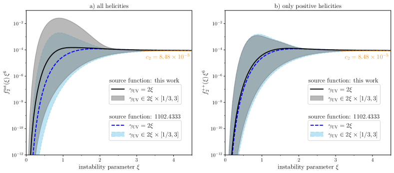
Figure 1: The function $f_{2}(\xi)$ parametrizing the gauge-field induced part of the scalar power spectrum, rescaled by the factor $\xi^{6}$, including contributions (a) from both circular polarizations of the gauge field, (b) only from the positive circular polarization which is exponentially enhanced w.r.t. the negative one. The black solid lines and gray shaded regions represent the results of full computation which takes into account the metric perturbations while the blue dashed line and light-blue shaded region correspond to the function $\tilde{f}_{2}(\xi)$ in the case when the metric perturbations are neglected. The thick black and blue lines correspond to the UV cutoff in the integral (114) at the instability scale, $\gamma_{{}_{\mathrm{UV}}}=2\xi$, while the shaded bands of the corresponding color show the variation of the final result under an increase or a decrease of the UV cutoff by a factor of 3. The orange dashed lines starting at $\xi=3$ show the leading term in the expansion of $f_{2}(\xi)$ in the large-$\xi$ approximation, see Eq. (119) and Appendix E.

V.2.1 Scalar power spectrum

We now compute the scalar power spectrum for inflation using Eq. (69). The second term in this equation, which describes the contribution induced by the presence of gauge fields, i.e., the inverse decay contribution, can be parametrized in the following form:

$$P_{\zeta}^{(\text{inv. dec.})}(k)=e^{4\pi\xi}\Big{(}\frac{H^{2}}{2\pi|\dot{\phi}_{c}|}\Big{)}^{4}f_{2}(\xi)\,,$$ (117)

where $f_{2}(\xi)$ is a dimensionless function introduced in Refs. [83, 84]. Using Eq. (113) and choosing $k$ (the only momentum scale) to be the overall momentum scale $q$, we find the following expression for the function $f_{2}(\xi)$:

$$f_{2}(\xi)=\frac{e^{-4\pi\xi}}{8\pi}\int d^{3}\bm{p}_{\ast}\sum\limits_{\lambda,\lambda^{\prime}=\pm}\Big{(}1-\lambda\lambda^{\prime}\frac{\bm{p}_{\ast}\cdot\bm{p}^{\prime}_{\ast}}{p_{\ast}p^{\prime}_{\ast}}\Big{)}^{2}p_{\ast}p^{\prime}_{\ast}\big{|}\mathcal{I}\big{(}\lambda,p_{\ast};\lambda^{\prime},p^{\prime}_{\ast};1\big{)}\big{|}^{2}\,,$$ (118)

where $\bm{p}^{\prime}_{\ast}=\hat{\bm{k}}-\bm{p}_{\ast}$, $\hat{\bm{k}}=\bm{k}/k$, the integral $\mathcal{I}$ is given by Eq. (114), and we used Eq. (217) for the scalar product of the polarization vectors.

In order to get some intuition about the analytic form of $f_{2}(\xi)$ and to compare with the well-known results in the literature, we first compute this function in the large-$\xi$ approximation in Appendix E. We call it an approximation because it is based on using the approximate expressions (218)–(219) for the gauge-field mode functions. These exponential functions are rather close to the exact solutions in Eqs. (98)–(102) but still never reproduce them exactly for arbitrarily large $\xi$. Moreover, only one circular polarization of the gauge field (the one which is amplified due to the axial coupling to the inflaton) is taken into account. Nevertheless, this approximation allows to compute the integral in Eq. (118) analytically in the form of a series in inverse powers of $\xi$. The leading term in this expansion behaves as

$$f_{2}(\xi)\simeq\frac{c_{2}}{\xi^{6}}$$ (119)

with the coefficient $c_{2}\approx$8.48\text{\times}{10}^{-5}$$, see Appendix E for more details. Note that this value of $c_{2}$ is about 12 larger than the one reported in Ref. [84] in the case when the metric perturbations are neglected.

We also compute the function $f_{2}(\xi)$ numerically for different values of $\xi$ and plot it rescaled by the factor of $\xi^{6}$ in Fig. 1. The rescaling compensates for the decrease of the function $f_{2}(\xi)$ in the region of large $\xi$. The black solid lines and the gray shaded regions around them represent the results of the computations which self-consistently include the metric perturbations while the blue dashed lines and the light-blue shaded regions show the results of the computations performed with the source term of Ref. [84] where the metric perturbations are neglected. Both the source terms are evaluated using the exact mode functions reported in Eqs. (98)–(102). The shaded bands show the variation of the corresponding results under a change of the UV cutoff in the integral in Eq. (114): the thick line in the middle corresponds to the reference value $\gamma_{{}_{\mathrm{UV}}}=2\xi$ which is the cutoff at the largest mode experiencing the tachyonic instability; the upper (lower) boundary of the shaded region corresponds to $\gamma_{{}_{\mathrm{UV}}}$ increased (decreased) by a factor of 3. Panel (a) shows the result including both circular polarizations of the gauge field while panel (b) shows the contribution of the positive polarization only. The orange dashed lines correspond to the leading term in the expansion over the inverse powers of $\xi$ derived in the large-$\xi$ approximation in Appendix E. Note that the number $c_{2}=$8.48\text{\times}{10}^{-5}$$ does not exactly coincide with the true asymptotic behavior of $\xi^{6}f_{2}(\xi)$ computed on the exact mode functions. But still, numerically, it appears to be rather close.

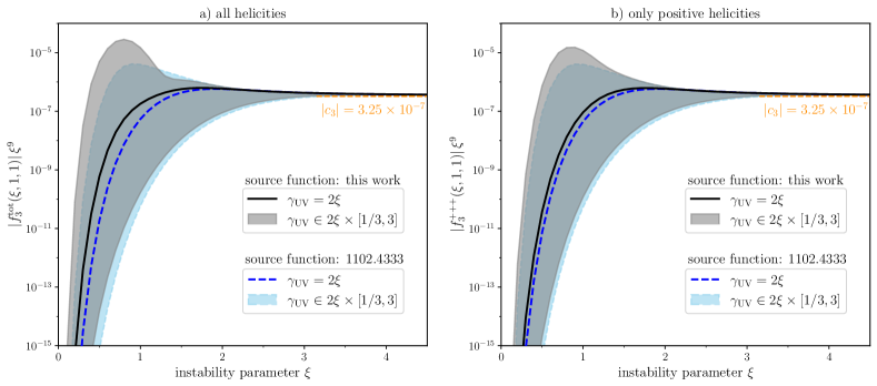
Figure 2: The function $f_{3}(\xi,1,1)$ parametrizing the equilateral scalar bispectrum rescaled by the factor of $\xi^{9}$, including contributions (a) from both circular polarizations of the gauge field, (b) only from the positive circular polarization which is exponentially enhanced w.r.t.  the negative one. The black solid lines and gray shaded regions represent the results of full computation which takes into account the metric perturbations while the blue dashed line and light-blue shaded region correspond to the function $\tilde{f}_{3}(\xi,1,1)$ in the case when the metric perturbations are neglected. The thick black and blue lines correspond to the UV cutoff in the integral (114) at the instability scale while the shaded bands of the corresponding color show the variation of the final result under an increase or a decrease of the UV cutoff by a factor of 3. The orange dashed lines show the leading term in the expansion of $f_{3}(\xi,1,1)$ in the large-$\xi$ approximation, see Eq. (122) and Appendix E.

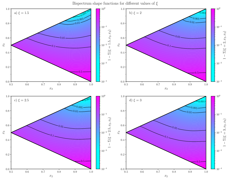
Figure 3: The bispectrum shape function $\Sigma(\xi,x_{2},x_{3})$ in the part of the $(x_{2},x_{3})$ plane limited by the inequalities (80) for four fixed values of $\xi$: (a) $\xi=1.5$, (b) $\xi=2$, (c) $\xi=2.5$, and (d) $\xi=3$. Since in all cases the shape function exhibits a broad maximum at the equilateral configuration, the color scheme and contour labels corresponds to the deviation of the shape function from unity, $1-\Sigma(\xi,x_{2},x_{3})$ in a logarithmic scale.

V.2.2 Scalar bispectrum

Let us now focus on the scalar bispectrum generated in the axion inflation model. Following Ref. [84], we introduce the function $f_{3}(\xi,\,x_{2},\,x_{3})$ defined by

$$\mathscr{B}_{\zeta}(k_{1},k_{2},k_{3})=\frac{3}{10}(2\pi)^{5/2}\Big{(}\frac{H^{2}}{2\pi|\dot{\phi}|}\Big{)}^{6}\frac{e^{6\pi\xi}}{k^{6}}\frac{1+x_{2}^{3}+x_{3}^{3}}{x_{2}^{3}x_{3}^{3}}f_{3}(\xi,\,x_{2},\,x_{3})\,.$$ (120)

Here, $k=k_{1}$ is the largest of the three momenta $k_{1}$, $k_{2}$, and $k_{3}$; the variables $x_{2}=k_{2}/k$ and $x_{3}=k_{3}/k$ satisfy the conditions detailed in Eq. (80).

Using Eq. (72) for the bispectrum, and substituting Eqs. (113) and (115), we arrive at the following expression for the function $f_{3}$:

$$f_{3}(\xi,x_{2},x_{3}) =-\frac{5}{3\pi}\frac{e^{-6\pi\xi}}{x_{2}x_{3}(1+x_{2}^{3}+x_{3}^{3})}\int d^{3}\bm{p}_{\ast}\sum\limits_{\lambda_{1},\lambda_{2},\lambda_{3}=\pm}p_{\ast}|\bm{p}_{\ast}-\hat{\bm{k}}_{1}||\hat{\bm{k}}_{3}x_{3}+\bm{p}_{\ast}|$$

$$\times\big{(}\bm{\epsilon}_{\lambda_{1}}(\bm{p}_{\ast})\cdot\bm{\epsilon}_{\lambda_{2}}(\hat{\bm{k}}_{1}-\bm{p}_{\ast})\big{)}\big{(}\bm{\epsilon}_{\lambda_{2}}(\bm{p}_{\ast}-\hat{\bm{k}}_{1})\cdot\bm{\epsilon}_{\lambda_{3}}(-\hat{\bm{k}}_{3}x_{3}-\bm{p}_{\ast})\big{)}\big{(}\bm{\epsilon}_{\lambda_{3}}(\hat{\bm{k}}_{3}x_{3}+\bm{p}_{\ast})\big{)}\cdot\bm{\epsilon}_{\lambda_{1}}(-\bm{p}_{\ast})\big{)}$$

$$\times\mathcal{I}\big{(}\lambda_{1},p_{\ast};\lambda_{2},|\bm{p}_{\ast}-\hat{\bm{k}}_{1}|;1\big{)}\mathcal{I}\big{(}(\lambda_{2},|\bm{p}_{\ast}-\hat{\bm{k}}_{1}|)^{\ast};\lambda_{3},|\hat{\bm{k}}_{3}x_{3}+\bm{p}_{\ast}|;x_{2}\big{)}\mathcal{I}\big{(}(\lambda_{3},|\hat{\bm{k}}_{3}x_{3}+\bm{p}_{\ast}|)^{\ast};(\lambda_{1},p_{\ast})^{\ast};x_{3}\big{)}\,,$$ (121)

where $\hat{\bm{k}}_{i}=\bm{k}_{i}/k_{i}$. We also used the relation (66) in order to express the function $K_{4}$ through $K_{1}$.

We first compute this function for the equilateral configuration, $x_{2}=x_{3}=1$. In the large-$\xi$ approximation, it behaves as

$$f_{3}(\xi,1,1)\simeq\frac{c_{3}(1,1)}{\xi^{9}}$$ (122)

with $c_{3}(1,1)\approx$-3.25\text{\times}{10}^{-7}$$; for more details, see Appendix E. Like for the power spectrum, this number is about 15 larger in absolute value than the corresponding quantity reported in Ref. [84] where the metric perturbations are neglected. Note the difference of the overall sign of the bispectrum compared to Refs. [83, 84] due to a different sign in the definition of the scalar perturbation variable $\zeta$; see also the footnote on page 9.

Further, we perform the numerical computations of the function $f_{3}(\xi,1,1)$ using the exact gauge-field mode functions. The results are shown in Fig. 2, where we rescaled $f_{3}(\xi,1,1)$ by a factor of $\xi^{9}$ in order to compensate for its decrease in the limit of large $\xi$ values. The color scheme and notations are exactly the same as in Fig. 1.

$\xi$	$\cos\Theta$ in Eq. (81) w.r.t. patterns:
	local (76)	equil. (77)	orth. (78)
$1.5$	$0.47$	$0.97$	$-0.10$
$2.0$	$0.47$	$0.97$	$-0.10$
$2.5$	$0.47$	$0.94$	$-0.10$
$3.0$	$0.49$	$0.94$	$-0.10$
large $\xi$	$0.51$	$0.92$	$-0.18$

Table 1: Cosines of the angles (81) between the shape functions $\Sigma(\xi,x_{2},x_{3})$ and the standard (local, equilateral, and orthogonal) patterns computed for four values of $\xi=1.5$, $2$, $2.5$, $3$ and in the large-$\xi$ approximation (see Appendix E). Note that, for the local case, $(\Sigma_{\mathrm{local}}\,,\Sigma_{\mathrm{local}})$ diverges and $\cos\Theta\to 0$ for $k_{\min}\to 0$. The value given in the table corresponds to the choice described in footnote 6.

The relative value of the bispectrum for arbitrary configurations of momenta compared to its value for the equilateral configuration is characterized by the shape function $\Sigma$ given by Eq. (75). It can be expressed in terms of the function $f_{3}$ as follows:

$$\Sigma(\xi,x_{2},x_{3})=\frac{1+x_{2}^{3}+x_{3}^{3}}{3x_{2}x_{3}}\frac{f_{3}(\xi,x_{2},x_{3})}{f_{3}(\xi,1,1)}\,.$$ (123)

We plot the shape functions for fixed values of $\xi=1.5$, $2$, $2.5$, and $3$ in the contour and density plots in Fig. 3. The shape functions exhibit a broad peak around the equilateral configuration; therefore, the numbers on the contours and the color scheme of the density plots correspond to the deviations of the shape functions from unity. The shape function is smallest in the local configuration, $x_{3}\to 0$. In these calculations, we used the reference value $\gamma_{{}_{\mathrm{UV}}}=2\xi$ for the UV cutoff. The shape function in the large-$\xi$ approximation is shown in Fig. 5 in Appendix E.

Finally, in order to see how similar the actual shape of non-Gaussianity is to the standard patterns (76)–(78), we compute the cosines of the angles between the obtained shape functions and the standard patterns using Eq. (81). They are listed in Table 1. The numbers show that the shape appears to be rather close to the equilateral pattern with the corresponding $\cos\Theta$ varying in the range from 0.92 in the large-$\xi$ approximation to 0.97 for small values of $\xi$.

V.3 Discussion

Even though in Ref. [84], only inflaton perturbations and the coupling of the inflaton to the gauge field were considered, and gravitational contributions to $\zeta$ were neglected, the final result agrees reasonably well with our more comprehensive treatment. We observe especially good agreement for $\xi\gtrsim 2$, where the black solid and blue dashed lines in Figs. 1 and 2 coincide almost perfectly (note that this accuracy is much better that the above mentioned 12–15 disagreement in the large-$\xi$ approximation). This remarkable agreement can be explained as follows. For moderate and large values of $\xi$, the dominant contribution to the functions $f_{2}$, $f_{3}$, as well as to any other quantity of interest in this paper, is made by the gauge-field modes with positive circular polarization; compare panels (a) and (b) in Figs. 1 and 2. The corresponding mode functions are highly peaked and take the largest values for $\rho\simeq 1/(8\xi)$; see Fig. 4 in Appendix E. Therefore, the maximal overlap of these peaked functions in the integral (114) occurs for the case $p_{\ast}\simeq p^{\prime}_{\ast}$ and quickly decreases when $p_{\ast}$ and $p^{\prime}_{\ast}$ become different. However, all differences between the new source term derived in the present work and the old one in Ref. [84] are proportional to the functions $h_{1}$, $h_{2}$, and $h_{3}$, which, in the slow-roll approximation, are given by Eqs. (109)–(111). Note that all three of them are proportional to $(\lambda p_{\ast}-\lambda^{\prime}p^{\prime}_{\ast})=(p_{\ast}-p^{\prime}_{\ast})$ or the same combination squared and, thus, vanish in the region $p_{\ast}\simeq p^{\prime}_{\ast}$, which is required for the maximal overlap of the mode functions.

Note that the above mentioned agreement is obtained in the simple case of axion inflation without backreaction where the slow-roll regime is realized. We expect that in other, physically more realistic and interesting cases, the effect of a self-consistent treatment of the metric perturbation may be important and may lead to $\mathcal{O}(1)$ corrections to the power spectrum and bispectrum. Especially interesting in this regard is the regime of strong gauge-field backreaction, whose background dynamics was studied, e.g., in Refs. [97, 109, 110, 108]. In this regime, at least two of the above-mentioned arguments are modified. Indeed, in the strong backreaction regime, the inflaton and the gauge-field background quantities exhibit oscillations during which the slow-roll conditions are violated, e.g., $\ddot{\phi}_{c}$ is as important as other terms in the Klein–Gordon equation. This means that the functions $h_{1}$, $h_{2}$, and $h_{3}$ will have other contributions which do not vanish for $p_{\ast}\simeq p^{\prime}_{\ast}$. Also, due to the oscillations, the peaks in the gauge-field mode functions may become broader, which will allow for a nonnegligible overlap in the integral (114) even for $p_{\ast}\neq p^{\prime}_{\ast}$. Furthermore, even the left-hand side of the differential equation for $\zeta$ will be strongly modified by the backreaction (modified in a different way than in the absence of metric perturbations). This will also lead to modifications in the vacuum contribution to the scalar power spectrum and consequently to a different expression for the Green’s function (47) which enters the power spectrum and bispectrum. The numerical study of perturbations in the strong-backreaction regime is much more involved compared to the case considered in the present article. We plan to address this problem in a future work.

The impact of the metric perturbations appears to be much more important for small values of $\xi$. Physically, this corresponds to early times during slow roll, when the cosmologically relevant scales exit the horizon. Here, one typically expects $\dot{\phi}_{c}/H$ to be very small so that $\xi$ may also be less than unity. In this case, the gauge-field amplification due to axial coupling is rather weak and the mode function is not as highly peaked as in the case of large $\xi$; see Fig. 4 in Appendix E. This means that the configurations of momenta with $p_{\ast}\neq p^{\prime}_{\ast}$ also make a significant contribution to the integral (114) and the new terms in the source proportional to the functions $h_{1}$, $h_{2}$, and $h_{3}$ become as important as the old source term. Note, however, that, in the region of small $\xi$, the numerical results presented in Figs. 1 and 2 are subject to considerable theoretical uncertainties for at least two different reasons. The first one is related to the UV cutoff in the integral $\mathcal{I}$ to which the functions $f_{2}$ and $f_{3}$ appear to be very sensitive. Although our reference value $\gamma_{{}_{\mathrm{UV}}}=2\xi$ is well motivated, the fact that even a mild change of this parameter within one order of magnitude leads to a large change in the numerical results spanning over 4–6 orders of magnitude, points towards the need for a more rigorous and accurate treatment of the UV divergence present in the problem. The second reason is related to the question of whether one has to take into account the contribution coming from the gauge-field mode functions of negative helicity, which appears to be comparable to that of the positive helicity in the region of small $\xi$. If we include it, it is unclear what the UV cutoff should be for these modes since they do not experience the tachyonic instability at all. In the present work, for definiteness, we took it to be the same as for the positive-helicity modes. Both issues can be resolved by employing a systematic QFT approach including conventional regularization and renormalization techniques. To the best of our knowledge, such an approach was only applied to the problem of gauge-field production during inflation in Ref. [134]. Undoubtedly, its application to the problem of induced scalar perturbations would require a separate, thorough investigation.

VI Conclusion and outlook

The production of gauge fields during inflation leads to new sources of cosmological perturbations. The slow roll of the inflaton amplifies the gauge fields, which in turn produce scalar fluctuations. These additional cosmological perturbations are statistically independent from the vacuum perturbations of the inflaton and can be highly non-Gaussian. Hence, for any scenario of inflation where gauge fields are generated, it is very important to keep track of the effect of these new source terms on the generation of scalar perturbations. Potentially, they can yield an additional contribution of perturbations which are both, non-Gaussian and, in general, not scale invariant. These properties are observable and can be used to constrain inflationary models that involve the production of gauge fields.

To the best of our knowledge, the majority of the current literature devoted to the investigation of this problem is based on the assumption that all the relevant effects arise from the coupling between the inflaton and the gauge fields while scalar metric perturbations are neglected (i.e., working with the unperturbed FLRW metric).

In the present work, we consider a generic model including the kinetic and axial coupling between the inflaton and an Abelian gauge field, and self-consistently take into account all scalar perturbations existing in the problem. Indeed, in the presence of arbitrary sources, the curvature perturbation variable is given by Eq. (41) and contains inflaton, metric, and source perturbations. In the absence of sources, this variable describes the curvature of the spatial sections in unitary gauge. We have derived a second order differential equation for the variable $\zeta$, Eq. (42), which is sourced by gauge-field perturbations. Standard inflationary predictions are obtained by simply setting the right hand side of this equation to zero.

Equation  (42) for the variable $\zeta$ is an inhomogeneous linear differential equation; therefore, its general solution consists of two parts. The first part represents the general solution of the corresponding homogeneous equation and describes the vacuum scalar perturbations arising on a homogeneous background which includes the inflaton as well as the gauge-field zero modes. The second part is induced by the source terms and corresponds to the scalar perturbations sourced by inhomogeneities in the gauge field. Note also that the sources $F_{\alpha}$ themselves evolve according to equations of motion which include $\zeta$. Hence, one may try to solve this coupled system of equations treating all perturbations on the same footing as, e.g., it is done with the adiabatic and the entropy modes in the multi-field inflationary models; see, e.g., Refs. [119, 120, 121]. However, since the gauge fields are already produced by the background inflaton motion, one may expect that the impact of scalar perturbations on the gauge-field evolution is small (provided that the former are small compared to the corresponding background quantities). In this work, we assume this and, as a first step, we neglect the impact of the inflaton and metric perturbations on the gauge-field mode functions. This allows us to derive closed expressions for the induced contributions to the scalar power spectrum and bispectrum given in Eqs. (69) and (72), respectively.

Although the main goal of this paper is to develop the formalism and to derive all equations needed to compute the scalar perturbations during inflation in the presence of the gauge field, in Sec. V, we apply our formalism to the well-known case of axion inflation neglecting backreaction. This case, which has been previously studied extensively, allows a comparison with the literature. For simplicity, we assume that the Hubble parameter $H$ as well as the gauge-field production parameter $\xi$ are both constant during inflation. This assumption allows us to solve the equations for the gauge-field mode functions and the Green’s function of the curvature perturbation analytically. We then use these in order to compute the induced scalar power spectrum and bispectrum. Comparing to Ref. [84], where metric perturbations are neglected, the source term in the equation for $\zeta$ (42) contains additional contributions. However, in the region of $\xi\gg 3$, the impact of extra terms is small and the power spectrum as well as the bispectrum (computed on the exact mode functions) arising from the sources in Ref. [84] and in the present work differ little, see Figs. 1 and 2. Nevertheless, we argue that this result strongly depends on the gauge-field mode functions. Indeed, if we use the approximate exponential form for the gauge-field mode function, we obtain a $\sim 10\,\%$ deviation between the our results and the ones of Ref. [84]. A larger disagreement is observed in the region of small $\xi\lesssim 2$. These deviations lead us to the conclusion that there is no fundamental reason for the impact of metric perturbations to be small, providing the main motivation for the revision of the formalism performed in this work.

A more interesting case, which potentially has many phenomenological applications, is the regime of strong backreaction of the gauge field on the background evolution. It is well known that the inflaton field and the gauge-field energy density both exhibit oscillatory behavior which is due to the delay between the moment of time when the gauge-field modes are enhanced and the moment of time they start to backreact on the expansion of the universe [135, 109, 108, 110]. It was shown that these oscillations lead to oscillatory features in the tensor power spectrum [136], which are potentially observable by space interferometers like LISA and by Pulsar Timing Arrays. Similar features are also expected to appear in the scalar power spectrum. Moreover, the periodic decrease of the inflaton velocity (sometimes even crossing zero) in the backreaction regime may lead to a strong enhancement of the vacuum scalar power spectrum, which can potentially lead to the creation of primordial black holes during radiation domination stage of universe. The formalism developed in our paper allows us to investigate these phenomena, which requires, as a first step, the computation of the scalar power spectrum and bispectrum of scalar fluctuations in the presence of backreaction. We intend to address these questions in more realistic physical models, including backreaction, with our new formalism in future studies.

Appendix A Details of the derivation of the perturbation equations

The components of the field-strength tensor read as

$$F_{0i} =a^{2}E^{i}\,,$$ (124)

$$F_{ij} =-a^{2}\varepsilon_{ijk}B^{k}\,,$$ (125)

$$F^{0i} =-\frac{1}{a^{2}}(1-2\Psi+2\Phi)E^{i}\,,$$ (126)

$$F^{ij} =-\frac{1}{a^{2}}(1+4\Phi)\varepsilon^{ijk}B^{k}\,.$$ (127)

The components of the dual tensor are given by

$$\tilde{F}^{0i} =-\frac{1}{a^{2}}(1-\Psi+3\Phi)B^{i}\,,$$ (128)

$$\tilde{F}^{ij} =\frac{1}{a^{2}}(1-\Psi+3\Phi)\varepsilon^{ijk}E^{k}\,.$$ (129)

$$\tilde{F}_{0i} =a^{2}(1+\Psi+\Phi)B^{i}\,,$$ (130)

$$\tilde{F}_{ij} =a^{2}(1-\Psi-\Phi)\varepsilon_{ijk}E^{k}\,,$$ (131)

The gauge-field invariants are of the form

$$(\!\!(F_{\mu\nu}F^{\mu\nu})\!\!)\! =2[(1+4\Phi)\bm{B}^{2}\!-\!(1-2\Psi+2\Phi)\bm{E}^{2}]\,,$$ (132)

$$(\!\!(F_{\mu\nu}\tilde{F}^{\mu\nu})\!\!)\! =-4(1-\Psi+3\Phi)(\!\!(\bm{E}\cdot\bm{B})\!\!)\,.$$ (133)

A.1 The Einstein tensor

The Einstein tensor in a linearly perturbed spatially flat FLRW universe in longitudinal gauge is given by

$$\langle G^{\ 0}_{0}\rangle = 3\frac{a^{\prime 2}}{a^{4}}=3\frac{\mathcal{H}^{2}}{a^{2}}\,,$$ (134)

$$\delta G^{\ 0}_{0} = \frac{2}{a^{2}}\big{[}\triangle\Phi-3\mathcal{H}\Phi^{\prime}-3\mathcal{H}^{2}\Psi\big{]}\,,$$ (135)

$$\langle G^{\ 0}_{i}\rangle = 0\,,$$ (136)

$$\delta G^{\ 0}_{i} = \frac{2}{a^{2}}\partial_{i}\big{[}\Phi^{\prime}+\mathcal{H}\Psi\big{]}\,,$$ (137)

$$\langle G_{\ j}^{i}\rangle = \delta_{j}^{i}\frac{1}{a^{2}}\left[2\frac{a^{\prime\prime}}{a}-\left(\frac{a^{\prime}}{a}\right)^{2}\right]=\delta_{j}^{i}\frac{1}{a^{2}}\big{[}2\mathcal{H}^{\prime}+\mathcal{H}^{2}\big{]}\,,$$ (138)

$$\delta G^{\ j}_{i} = -\frac{1}{a^{2}}\partial_{i}\partial_{j}(\Phi-\Psi)-\frac{2}{a^{2}}\delta_{j}^{i}\bigg{\{}\Phi^{\prime\prime}+\frac{1}{2}\triangle(\Psi\!-\!\Phi)\!+\!\mathcal{H}(\Psi^{\prime}\!+\!2\Phi^{\prime})+(2\mathcal{H}^{\prime}\!+\!\mathcal{H}^{2})\Psi\bigg{\}}\,,$$ (139)

where $\langle G^{\mu}_{\nu}\rangle$ are the background quantities.

A.2 The energy–momentum tensor

The energy–momentum tensor (2) can be represented as $T_{\mu}^{\ \nu}=\langle T_{\mu}^{\ \nu}\rangle+\delta T_{\mu}^{\ \nu}$, where

$$\langle T^{0}_{\ 0}\rangle =\frac{\phi_{c}^{\prime 2}}{2a^{2}}+V(\phi_{c})+\frac{1}{2}I_{1}(\phi_{c})\Big{[}\langle\bm{E}^{2}\rangle+\langle\bm{B}^{2}\rangle\Big{]}\,,$$ (140)

$$\delta T^{0}_{\ 0} =\frac{\phi^{\prime}_{c}}{a^{2}}\delta\varphi^{\prime}+\Big{[}V^{\prime}(\phi_{c})+\frac{1}{2}I^{\prime}_{1}(\phi_{c})\Big{(}\langle\bm{E}^{2}\rangle+\langle\bm{B}^{2}\rangle\Big{)}\Big{]}\delta\varphi+\frac{1}{2}I_{1}(\phi_{c})\Big{[}\delta_{\bm{E}^{2}}+\delta_{\bm{B}^{2}}\Big{]}-\frac{\phi_{c}^{\prime 2}}{a^{2}}\Psi$$

$$\qquad+I_{1}(\phi_{c})\Big{[}(\Phi-\Psi)\langle\bm{E}^{2}\rangle+2\Phi\langle\bm{B}^{2}\rangle\Big{]}\,,$$ (141)

$$\langle T_{i}^{\ 0}\rangle =\langle T_{0}^{\ i}\rangle=0\,,$$ (142)

$$\delta T_{i}^{\ 0} =-\delta T_{0}^{\ i}=\frac{\phi^{\prime}_{c}}{a^{2}}\partial_{i}\delta\varphi-I_{1}(\phi_{c})\varepsilon_{ijk}\delta_{E_{j}B_{k}}\,,$$ (143)

$$\langle T_{i}^{\ j}\rangle =-\delta_{i}^{j}\bigg{[}\frac{\phi_{c}^{\prime 2}}{2a^{2}}-V(\phi_{c})+\frac{1}{6}I_{1}(\phi_{c})\Big{(}\langle\bm{E}^{2}\rangle+\langle\bm{B}^{2}\rangle\Big{)}\bigg{]}\,,$$ (144)

$$\delta T_{i}^{\ j} =I_{1}(\phi_{c})\left[\delta_{E_{i}E_{j}}+\delta_{B_{i}B_{j}}\right]-\delta_{i}^{j}\bigg{\{}\frac{\phi^{\prime}_{c}}{a^{2}}\delta\varphi^{\prime}+\Big{[}-V^{\prime}(\phi_{c})+\frac{1}{6}I^{\prime}_{1}(\phi_{c})\Big{(}\langle\bm{E}^{2}\rangle+\langle\bm{B}^{2}\rangle\Big{)}\Big{]}\delta\varphi$$

$$\qquad-\frac{\phi_{c}^{\prime 2}}{a^{2}}\Psi+\frac{1}{3}I_{1}(\phi_{c})\Big{[}(\Phi-\Psi)\langle\bm{E}^{2}\rangle+2\Phi\langle\bm{B}^{2}\rangle\Big{]}+\frac{1}{2}I_{1}(\phi_{c})\Big{[}\delta_{\bm{E}^{2}}+\delta_{\bm{B}^{2}}\Big{]}\bigg{\}}\,.$$ (145)

With the aim to extract only the scalar contribution to the energy-momentum tensor, we introduce the scalar gauge-field sources in Eqs. (23)–(26), where $\delta T^{\ \nu\,\mathrm{(EM)}}_{\mu}$ is the part of the energy–momentum tensor perturbation containing gauge-field perturbations, e.g., $\delta_{E_{i}E_{j}}$ etc. Applying the corresponding projectors, we eventually get the following expressions:

$$\delta T^{\ 0\,\mathrm{(s)}}_{0} =\delta T^{\ 0}_{0}=\frac{\phi^{\prime}_{c}}{a^{2}}\delta\varphi^{\prime}+\Big{[}V^{\prime}(\phi_{c})+\frac{1}{2}I^{\prime}_{1}(\phi_{c})\Big{(}\langle\bm{E}^{2}\rangle+\langle\bm{B}^{2}\rangle\Big{)}\Big{]}\delta\varphi-\Big{[}\frac{\phi^{\prime 2}_{c}}{a^{2}}+I_{1}(\phi_{c})\langle\bm{E}^{2}\rangle\Big{]}\Psi$$

$$\hskip 256.0748pt+I_{1}(\phi_{c})\Big{[}\langle\bm{E}^{2}\rangle+2\langle\bm{B}^{2}\rangle\Big{]}\Phi+\frac{2M_{\mathrm{P}}^{2}}{a^{2}}F_{\rho}\,,$$ (146)

$$\delta T^{\ 0\,\mathrm{(s)}}_{i} =\frac{\partial_{i}\partial_{j}}{\triangle}\delta T^{\ 0}_{j}=\partial_{i}\Big{[}\frac{\phi^{\prime}_{c}}{a^{2}}\delta\varphi+\frac{2M_{\mathrm{P}}^{2}}{a^{2}}F_{v}\Big{]}\,,$$ (147)

$$\delta T^{\ j\,\mathrm{(s)}}_{i} =-\delta^{j}_{i}\bigg{\{}\frac{\phi^{\prime}_{c}}{a^{2}}\delta\varphi^{\prime}+\Big{[}-V^{\prime}(\phi_{c})+\frac{1}{6}I^{\prime}_{1}(\phi_{c})\Big{(}\langle\bm{E}^{2}\rangle+\langle\bm{B}^{2}\rangle\Big{)}\Big{]}\delta\varphi-\Big{[}\frac{\phi^{\prime 2}_{c}}{a^{2}}+\frac{1}{3}I_{1}(\phi_{c})\langle\bm{E}^{2}\rangle\Big{]}\Psi$$

$$\hskip 156.49014pt+\frac{1}{3}I_{1}(\phi_{c})\Big{[}\langle\bm{E}^{2}\rangle+2\langle\bm{B}^{2}\rangle\Big{]}\Phi+f_{p}\bigg{\}}-\Big{(}\partial_{i}\partial_{j}-\frac{2M_{\mathrm{P}}^{2}}{a^{2}}\frac{1}{3}\delta^{j}_{i}\triangle\Big{)}F_{\pi}\,.$$ (148)

Combining Eqs. (135), (137), and (139) with Eqs. (146)–(148) into the perturbed Einstein equations $\delta G_{\mu}^{\ \nu}=M_{\mathrm{P}}^{-2}\delta T_{\mu}^{\ \nu}$, we obtain Eqs. (27)–(30) in the main text.

Appendix B Details of the derivation of the equation for the curvature perturbation $\zeta$-variable

B.1 The $\zeta$ equation

In order to derive the equation for the variable $\zeta$, one should follow the next steps:

• Step 1. Substituting $\Psi=\Phi-2F_{\pi}$ into Eq. (III.1) in the Fourier space (i.e., replacing $\triangle\to-k^{2}$), we solve it with respect to $\delta\varphi^{\prime}$ and obtain the following result:

  $$\delta\varphi^{\prime}=\frac{2M_{\mathrm{P}}^{2}}{\phi^{\prime}_{c}}\bigg{\{}\Big{[}-k^{2}+\frac{\phi^{\prime 2}_{c}}{2M_{\mathrm{P}}^{2}}-\frac{a^{2}}{M_{\mathrm{P}}^{2}}I_{1}(\phi_{c})\langle\bm{B}^{2}\rangle\Big{]}\Phi-\frac{1}{2M_{\mathrm{P}}^{2}}\Big{[}3\mathcal{H}\phi^{\prime}_{c}+a^{2}V^{\prime}(\phi_{c})+\frac{1}{2}a^{2}I^{\prime}_{1}(\phi_{c})\big{(}\langle\bm{E}^{2}\rangle+\langle\bm{B}^{2}\rangle\big{)}\Big{]}\delta\varphi\\ -F_{\rho}-3\mathcal{H}F_{v}-\Big{[}\frac{\phi^{\prime 2}_{c}}{M_{\mathrm{P}}^{2}}+\frac{a^{2}}{M_{\mathrm{P}}^{2}}I_{1}(\phi_{c})\langle\bm{E}^{2}\rangle\Big{]}F_{\pi}\bigg{\}}\,.$$ (149)

• Step 2. Substituting $\Psi=\Phi-2F_{\pi}$ into Eq. (28), we solve it with respect to $\Phi^{\prime}$ and obtain the following result:

  $$\Phi^{\prime}=-\mathcal{H}\Phi+\frac{\phi^{\prime}_{c}}{2M_{\mathrm{P}}^{2}}\delta\varphi+F_{v}+2\mathcal{H}F_{\pi}\,.$$ (150)

• Step 3. Using Eq. (29), we determine the combination $(\Phi^{\prime}+\mathcal{H}\Psi)^{\prime}=\Phi^{\prime\prime}+\mathcal{H}\Psi^{\prime}+\mathcal{H}^{\prime}\Psi$:

  $$\Phi^{\prime\prime}+\mathcal{H}\Psi^{\prime}+\mathcal{H}^{\prime}\Psi=-2\mathcal{H}\Phi^{\prime}-(\mathcal{H}^{\prime}+\mathcal{H}^{2})\Psi+\frac{a^{2}}{2M_{\mathrm{P}}^{2}}\bigg{\{}\frac{\phi^{\prime}_{c}}{a^{2}}\delta\varphi^{\prime}+\Big{[}-V^{\prime}(\phi_{c})+\frac{1}{6}I^{\prime}_{1}(\phi_{c})\Big{(}\langle\bm{E}^{2}\rangle+\langle\bm{B}^{2}\rangle\Big{)}\Big{]}\delta\varphi\\ -\Big{[}\frac{\phi^{\prime 2}_{c}}{a^{2}}+\frac{1}{3}I_{1}(\phi_{c})\langle\bm{E}^{2}\rangle\Big{]}\Psi+\frac{1}{3}I_{1}(\phi_{c})\Big{[}\langle\bm{E}^{2}\rangle+2\langle\bm{B}^{2}\rangle\Big{]}\Phi\bigg{\}}+\frac{1}{3}F_{p}-\frac{2}{3}k^{2}F_{\pi}\,.$$ (151)

  Substituting also here $\Psi=\Phi-2F_{\pi}$ and Eq. (150), we obtain the following result:

  $$(\Phi^{\prime}+\mathcal{H}\Psi)^{\prime}=\Big{[}-k^{2}+\frac{\phi^{\prime 2}_{c}}{2M_{\mathrm{P}}^{2}}+\frac{a^{2}}{3M_{\mathrm{P}}^{2}}I_{1}(\phi_{c})\big{(}\langle\bm{E}^{2}\rangle-\langle\bm{B}^{2}\rangle\big{)}\Big{]}\Phi-\frac{1}{2M_{\mathrm{P}}^{2}}\Big{[}5\mathcal{H}\phi^{\prime}_{c}+2a^{2}V^{\prime}(\phi_{c})+\frac{a^{2}}{3}I^{\prime}_{1}(\phi_{c})\big{(}\langle\bm{E}^{2}\rangle+\langle\bm{B}^{2}\rangle\big{)}\Big{]}\delta\varphi\\ -\frac{2}{3}F_{\rho}-5\mathcal{H}F_{v}-\Big{[}\frac{2}{3}k^{2}+\frac{\phi^{\prime 2}_{c}}{M_{\mathrm{P}}^{2}}+\frac{2a^{2}}{3M_{\mathrm{P}}^{2}}I_{1}(\phi_{c})\big{(}2\langle\bm{E}^{2}\rangle+\langle\bm{B}^{2}\rangle\big{)}\Big{]}F_{\pi}\,.$$ (152)

  The same expression can also be obtained by direct differentiation of Eq. (28) and substituting $F^{\prime}_{v}$ from Eq. (37), $\delta\varphi^{\prime}$ from Eq. (149), and $\phi^{\prime\prime}_{c}$ from Eq. (11).

• Step 4. Equation (41) can be represented in the following form:

  $$\zeta=M_{11}\Phi+M_{12}\delta\varphi+c_{1}^{(\rho)}F_{\rho}+c_{1}^{(v)}F_{v}+c_{1}^{(\pi)}F_{\pi}\,,$$ (153)

  where

  $$M_{11}=1,\qquad M_{12}=\frac{\mathcal{H}}{\mathcal{H}^{2}-\mathcal{H}^{\prime}}\frac{\phi^{\prime}_{c}}{2M_{\mathrm{P}}^{2}},\qquad c_{1}^{(\rho)}=c_{1}^{(\pi)}=0,\qquad c_{1}^{(v)}=\frac{\mathcal{H}}{\mathcal{H}^{2}-\mathcal{H}^{\prime}}\,.$$ (154)

  We want to represent $\zeta^{\prime}$ in a similar form. For this, we take the time derivative of the right-hand side of Eq. (40) and use Eqs. (150) and (152) to get rid of the derivatives of the perturbation variables. We obtain

  $$\zeta^{\prime}=M_{21}\Phi+M_{22}\delta\varphi+c_{2}^{(\rho)}F_{\rho}+c_{2}^{(v)}F_{v}+c_{2}^{(\pi)}F_{\pi}\,,$$ (155)

  with

  $$M_{21} =-\frac{\mathcal{H}}{\mathcal{H}^{2}-\mathcal{H}^{\prime}}\Big{[}k^{2}+\frac{2a^{2}}{3M_{\mathrm{P}}^{2}}I_{1}(\phi_{c})\langle\bm{B}^{2}\rangle\big{)}\Big{]}\,,$$ (156)

  $$M_{22} =-\frac{\mathcal{H}}{M_{\mathrm{P}}^{2}(\mathcal{H}^{2}-\mathcal{H}^{\prime})^{2}}\bigg{\{}\frac{\phi^{\prime 2}_{c}a^{2}}{6M_{\mathrm{P}}^{2}}\big{[}I^{\prime}_{1}(\phi_{c})\langle\bm{E}^{2}\rangle+I^{\prime}_{2}(\phi_{c})\langle(\!\!(\bm{E}\cdot\bm{B})\!\!)\rangle\big{]}$$

  $$\hskip 85.35826pt+\frac{a^{2}}{3M_{\mathrm{P}}^{2}}I_{1}(\phi_{c})\big{(}\langle\bm{E}^{2}\rangle+\langle\bm{B}^{2}\rangle\big{)}\,\Big{[}\mathcal{H}\phi^{\prime}_{c}+a^{2}V^{\prime}(\phi_{c})+\frac{a^{2}}{6}I^{\prime}_{1}(\phi_{c})\big{(}\langle\bm{E}^{2}\rangle+\langle\bm{B}^{2}\rangle\big{)}\Big{]}\bigg{\}}\,,$$ (157)

  $$c_{2}^{(\rho)} =-\frac{2}{3}\frac{\mathcal{H}}{\mathcal{H}^{2}-\mathcal{H}^{\prime}}\,,$$ (158)

  $$c_{2}^{(\pi)} =-\frac{2}{3}\frac{\mathcal{H}}{\mathcal{H}^{2}-\mathcal{H}^{\prime}}\Big{[}k^{2}+\frac{a^{2}}{M_{\mathrm{P}}^{2}}I_{1}(\phi_{c})\langle\bm{E}^{2}\rangle\Big{]}\,,$$ (159)

  $$c_{2}^{(v)} =1+\Big{(}\frac{\mathcal{H}}{\mathcal{H}^{2}-\mathcal{H}^{\prime}}\Big{)}^{\prime}-5\frac{\mathcal{H}^{2}}{\mathcal{H}^{2}-\mathcal{H}^{\prime}}=\frac{\mathcal{H}a^{2}}{M_{\mathrm{P}}^{2}(\mathcal{H}^{2}-\mathcal{H}^{\prime})^{2}}\bigg{\{}\phi^{\prime}_{c}\Big{[}V^{\prime}(\phi_{c})-\frac{1}{6}I^{\prime}_{1}(\phi_{c})\big{(}\langle\bm{E}^{2}\rangle-\langle\bm{B}^{2}\rangle\big{)}$$

  $$\hskip 199.16928pt-\frac{1}{3}I^{\prime}_{2}(\phi_{c})\langle(\!\!(\bm{E}\cdot\bm{B})\!\!)\rangle\Big{]}-\frac{2}{3}\mathcal{H}I_{1}(\phi_{c})\big{(}\langle\bm{E}^{2}\rangle+\langle\bm{B}^{2}\rangle\big{)}\bigg{\}}\,.$$ (160)

• Step 5. Solving Eqs. (153) and (155) for $\Phi$ and $\delta\varphi$, we find the following results:

  $$\Phi =\big{(}M^{-1}\big{)}_{11}\zeta+\big{(}M^{-1}\big{)}_{12}\zeta^{\prime}-\sum_{\alpha=\rho,\pi,v}\Big{[}\big{(}M^{-1}\big{)}_{11}c_{1}^{(\alpha)}+\big{(}M^{-1}\big{)}_{12}c_{2}^{(\alpha)}\Big{]}F_{\alpha}\,,$$ (161)

  $$\delta\varphi =\big{(}M^{-1}\big{)}_{21}\zeta+\big{(}M^{-1}\big{)}_{22}\zeta^{\prime}-\sum_{\alpha=\rho,\pi,v}\Big{[}\big{(}M^{-1}\big{)}_{21}c_{1}^{(\alpha)}+\big{(}M^{-1}\big{)}_{22}c_{2}^{(\alpha)}\Big{]}F_{\alpha}\,,$$ (162)

  where $M^{-1}$ denotes the inverse matrix of the matrix $M$.

• Step 6. We now take the time derivative of Eq. (155):

  $$\zeta^{\prime\prime}=M_{21}\Phi^{\prime}+M^{\prime}_{21}\Phi+M_{22}\delta\varphi^{\prime}+M^{\prime}_{22}\delta\varphi+\sum_{\alpha=\rho,\pi,v}\big{[}c_{2}^{(\alpha)}F^{\prime}_{\alpha}+(c_{2}^{(\alpha)})^{\prime}F_{\alpha}\big{]}\,.$$ (163)

  Inserting Eqs. (150), (149), and the equations of motion for the sources Eqs. (36) and (37) in (163), we can express $\zeta^{\prime\prime}$ in terms of $\Phi$, $\varphi$, and the sources $F_{\alpha}$, $F^{\prime}_{\pi}$, $\delta_{\bm{E}^{2}}$, and $\delta_{\bm{E}\cdot\bm{B}}$ as follows:

  $$\zeta^{\prime\prime}=d^{(\Phi)}\Phi+d^{(\delta\varphi)}\delta\varphi+d^{(v)}F_{v}+d^{(\rho)}F_{\rho}+d^{(\pi)}_{1}F_{\pi}+d^{(\pi)}_{2}F^{\prime}_{\pi}+d^{(\bm{E}^{2})}\delta_{\bm{E}^{2}}+d^{(\bm{E}\cdot\bm{B})}\delta_{\bm{E}\cdot\bm{B}}\,,$$ (164)

  where

  $$d^{(\Phi)} =M^{\prime}_{21}-\mathcal{H}M_{21}+\frac{2M_{\mathrm{P}}^{2}}{\phi^{\prime}_{c}}\Big{[}-k^{2}+\frac{\phi^{\prime 2}_{c}}{2M_{\mathrm{P}}^{2}}-\frac{a^{2}}{M_{\mathrm{P}}^{2}}I_{1}(\phi_{c})\langle\bm{B}^{2}\rangle\Big{]}M_{22}+\frac{a^{2}}{3M_{\mathrm{P}}^{2}}I_{1}(\phi_{c})\big{(}\langle\bm{E}^{2}\rangle+2\langle\bm{B}^{2}\rangle\big{)}c_{2}^{(v)}$$

  $$+\bigg{\{}\frac{a^{2}}{\phi^{\prime}_{c}}\big{[}I^{\prime}_{1}(\phi_{c})\langle\bm{E}^{2}\rangle+I^{\prime}_{2}(\phi_{c})\langle(\!\!(\bm{E}\cdot\bm{B})\!\!)\rangle\big{]}\Big{[}k^{2}+\frac{a^{2}}{M_{\mathrm{P}}^{2}}I_{1}(\phi_{c})\langle\bm{B}^{2}\rangle\Big{]}-\frac{a^{2}\phi^{\prime}_{c}}{2M_{\mathrm{P}}^{2}}\big{[}I^{\prime}_{1}(\phi_{c})\langle\bm{E}^{2}\rangle+3I^{\prime}_{2}(\phi_{c})\langle(\!\!(\bm{E}\cdot\bm{B})\!\!)\rangle\big{]}$$

  $$\hskip 227.62204pt-\frac{a^{2}}{M_{\mathrm{P}}^{2}}I_{1}(\phi_{c})\big{[}\mathcal{H}\langle\bm{E}^{2}\rangle-2\langle(\!\!(\bm{E}\cdot\operatorname{rot}\bm{B})\!\!)\rangle\big{]}\bigg{\}}c_{2}^{(\rho)}\,,$$ (165)

  $$d^{(\delta\varphi)} =M^{\prime}_{22}+\frac{\phi^{\prime}_{c}}{2M_{\mathrm{P}}^{2}}M_{21}-\Big{[}3\mathcal{H}+\frac{a^{2}}{\phi^{\prime}_{c}}V^{\prime}(\phi_{c})+\frac{a^{2}}{2\phi^{\prime}_{c}}I^{\prime}_{1}(\phi_{c})\big{(}\langle\bm{E}^{2}\rangle+\langle\bm{B}^{2}\rangle\big{)}\Big{]}M_{22}$$

  $$-\frac{a^{2}}{6M_{\mathrm{P}}^{2}}\big{[}I^{\prime}_{1}(\phi_{c})\big{(}\langle\bm{E}^{2}\rangle-2\langle\bm{B}^{2}\rangle\big{)}+3I^{\prime}_{2}(\phi_{c})\langle(\!\!(\bm{E}\cdot\bm{B})\!\!)\rangle\big{]}c_{2}^{(v)}$$

  $$+\frac{a^{2}}{2M_{\mathrm{P}}^{2}}\bigg{\{}\big{[}I^{\prime}_{1}(\phi_{c})\langle\bm{E}^{2}\rangle+I^{\prime}_{2}(\phi_{c})\langle(\!\!(\bm{E}\cdot\bm{B})\!\!)\rangle\big{]}\Big{[}3\mathcal{H}+\frac{a^{2}}{\phi^{\prime}_{c}}V^{\prime}(\phi_{c})+\frac{a^{2}}{2\phi^{\prime}_{c}}I^{\prime}_{1}(\phi_{c})\big{(}\langle\bm{E}^{2}\rangle+\langle\bm{B}^{2}\rangle\big{)}\Big{]}$$

  $$-\phi^{\prime}_{c}\Big{[}\Big{(}I^{\prime\prime}_{1}(\phi_{c})-\frac{I^{\prime 2}_{1}(\phi_{c})}{I_{1}(\phi_{c})}\Big{)}\langle\bm{E}^{2}\rangle+\Big{(}I^{\prime\prime}_{2}(\phi_{c})-\frac{I^{\prime}_{1}(\phi_{c})I^{\prime}_{2}(\phi_{c})}{I_{1}(\phi_{c})}\Big{)}\langle(\!\!(\bm{E}\cdot\bm{B})\!\!)\rangle\Big{]}+\frac{\phi^{\prime}_{c}}{M_{\mathrm{P}}^{2}}I_{1}(\phi_{c})\langle\bm{E}^{2}\rangle\bigg{\}}c_{2}^{(\rho)}\,,$$ (166)

  $$d^{(v)} =c_{2}^{(v)\prime}-2\mathcal{H}c_{2}^{(v)}+M_{21}-\frac{6M_{\mathrm{P}}^{2}\mathcal{H}}{\phi^{\prime}_{c}}M_{22}+\Big{\{}-k^{2}+\frac{a^{2}}{M_{\mathrm{P}}^{2}}I_{1}(\phi_{c})\langle\bm{E}^{2}\rangle+\frac{3\mathcal{H}a^{2}}{\phi^{\prime}_{c}}\big{[}I^{\prime}_{1}(\phi_{c})\langle\bm{E}^{2}\rangle$$

  $$\hskip 298.75394pt+I^{\prime}_{2}(\phi_{c})\langle(\!\!(\bm{E}\cdot\bm{B})\!\!)\rangle\big{]}\Big{\}}c_{2}^{(\rho)}\,,$$ (167)

  $$d^{(\rho)} =c_{2}^{(\rho)\prime}+\Big{\{}-2\mathcal{H}+\frac{I^{\prime}_{1}(\phi_{c})}{I_{1}(\phi_{c})}\phi^{\prime}_{c}+\frac{a^{2}}{\phi^{\prime}_{c}}\big{[}I^{\prime}_{1}(\phi_{c})\langle\bm{E}^{2}\rangle+I^{\prime}_{2}(\phi_{c})\langle(\!\!(\bm{E}\cdot\bm{B})\!\!)\rangle\big{]}\Big{\}}c_{2}^{(\rho)}+\frac{1}{3}c_{2}^{(v)}-\frac{2M_{\mathrm{P}}^{2}}{\phi^{\prime}_{c}}M_{22}\,,$$ (168)

  $$d^{(\pi)}_{1} =c_{2}^{(\pi)\prime}+2\mathcal{H}M_{21}-\Big{[}2\phi^{\prime}_{c}+\frac{2a^{2}}{\phi^{\prime}_{c}}I_{1}(\phi_{c})\langle\bm{E}^{2}\rangle\Big{]}M_{22}-\Big{[}\frac{2}{3}k^{2}+\frac{a^{2}}{3M_{\mathrm{P}}^{2}}I_{1}(\phi_{c})\big{(}\langle\bm{E}^{2}\rangle+2\langle\bm{B}^{2}\rangle\big{)}\Big{]}c_{2}^{(v)}$$

  $$+\frac{a^{2}}{M_{\mathrm{P}}^{2}}\Big{\{}\phi^{\prime}_{c}\big{[}I^{\prime}_{1}(\phi_{c})\langle\bm{E}^{2}\rangle+2I^{\prime}_{2}(\phi_{c})\langle(\!\!(\bm{E}\cdot\bm{B})\!\!)\rangle\big{]}+\frac{a^{2}}{\phi^{\prime}_{c}}I_{1}(\phi_{c})\langle\bm{E}^{2}\rangle\big{[}I^{\prime}_{1}(\phi_{c})\langle\bm{E}^{2}\rangle+I^{\prime}_{2}(\phi_{c})\langle(\!\!(\bm{E}\cdot\bm{B})\!\!)\rangle\big{]}$$

  $$\hskip 241.84842pt+2I_{1}(\phi_{c})\big{[}\mathcal{H}\langle\bm{E}^{2}\rangle-\langle(\!\!(\bm{E}\cdot\operatorname{rot}\bm{B})\!\!)\rangle\big{]}\Big{\}}c_{2}^{(\rho)}\,,$$ (169)

  $$d^{(\pi)}_{2} =c_{2}^{(\pi)}-\frac{a^{2}}{M_{\mathrm{P}}^{2}}I_{1}(\phi_{c})\langle\bm{E}^{2}\rangle c_{2}^{(\rho)}=-\frac{2k^{2}}{3}\frac{\mathcal{H}}{\mathcal{H}^{2}-\mathcal{H}^{\prime}}\,,$$ (170)

  $$d^{(\bm{E}^{2})} =-\frac{a^{2}\phi^{\prime}_{c}}{2M_{\mathrm{P}}^{2}}I^{\prime}_{1}(\phi_{c})c_{2}^{(\rho)}=\frac{a^{2}I^{\prime}_{1}(\phi_{c})\phi^{\prime}_{c}}{3M_{\mathrm{P}}^{2}}\frac{\mathcal{H}}{\mathcal{H}^{2}-\mathcal{H}^{\prime}}\,,$$ (171)

  $$d^{(\bm{E}\cdot\bm{B})} =-\frac{a^{2}\phi^{\prime}_{c}}{2M_{\mathrm{P}}^{2}}I^{\prime}_{2}(\phi_{c})c_{2}^{(\rho)}=\frac{a^{2}I^{\prime}_{2}(\phi_{c})\phi^{\prime}_{c}}{3M_{\mathrm{P}}^{2}}\frac{\mathcal{H}}{\mathcal{H}^{2}-\mathcal{H}^{\prime}}\,.$$ (172)

  Finally, we use Eqs. (161)–(162) to write an equation of motion for the $\zeta$ variable alone in the following form:

  $$\zeta^{\prime\prime}+p\zeta^{\prime}+q\zeta=r^{(v)}F_{v}+r^{(\rho)}F_{\rho}+\\ +r^{(\pi)}_{1}F_{\pi}+r^{(\pi)}_{2}F^{\prime}_{\pi}+r^{(\bm{E}^{2})}\delta_{\bm{E}^{2}}+r^{(\bm{E}\cdot\bm{B})}\delta_{\bm{E}\cdot\bm{B}}\,,$$ (173)

  where

  $$p =-\big{(}M^{-1}\big{)}_{12}d^{(\Phi)}-\big{(}M^{-1}\big{)}_{22}d^{(\delta\varphi)}\,,$$ (174)

  $$q =-\big{(}M^{-1}\big{)}_{11}d^{(\Phi)}-\big{(}M^{-1}\big{)}_{21}d^{(\delta\varphi)}\,,$$ (175)

  $$r^{(v)} =d^{(v)}-\Big{[}\big{(}M^{-1}\big{)}_{11}c_{1}^{(v)}+\big{(}M^{-1}\big{)}_{12}c_{2}^{(v)}\Big{]}d^{(\Phi)}-\Big{[}\big{(}M^{-1}\big{)}_{21}c_{1}^{(v)}+\big{(}M^{-1}\big{)}_{22}c_{2}^{(v)}\Big{]}d^{(\delta\varphi)}\,,$$ (176)

  $$r^{(\rho)} =d^{(\rho)}-\Big{[}\big{(}M^{-1}\big{)}_{11}c_{1}^{(\rho)}+\big{(}M^{-1}\big{)}_{12}c_{2}^{(\rho)}\Big{]}d^{(\Phi)}-\Big{[}\big{(}M^{-1}\big{)}_{21}c_{1}^{(\rho)}+\big{(}M^{-1}\big{)}_{22}c_{2}^{(\rho)}\Big{]}d^{(\delta\varphi)}\,,$$ (177)

  $$r^{(\pi)}_{1} =d^{(\pi)}_{1}-\Big{[}\big{(}M^{-1}\big{)}_{11}c_{1}^{(\pi)}+\big{(}M^{-1}\big{)}_{12}c_{2}^{(\pi)}\Big{]}d^{(\Phi)}-\Big{[}\big{(}M^{-1}\big{)}_{21}c_{1}^{(\pi)}+\big{(}M^{-1}\big{)}_{22}c_{2}^{(\pi)}\Big{]}d^{(\delta\varphi)}\,,$$ (178)

  $$r^{(\pi)}_{2} =d^{(\pi)}_{2}\,,\qquad r^{(\bm{E}^{2})}=d^{(\bm{E}^{2})}\,,\qquad r^{(\bm{E}\cdot\bm{B})}=d^{(\bm{E}\cdot\bm{B})}\,.$$ (179)

B.2 Particular case: axion inflation in the absence of backreaction

In Section V, we apply our formalism to axion inflation, where $I_{1}=1$, neglecting backreaction. In this case our general $\zeta$-equation simplifies as follows:

$$\zeta^{\prime\prime}+2\Big{(}\frac{\phi^{\prime\prime}_{c}}{\phi^{\prime}_{c}}-\frac{\mathcal{H}^{\prime}}{\mathcal{H}}+\mathcal{H}\Big{)}\zeta^{\prime}+k^{2}\zeta=r^{(v)}F_{v}+r^{(\rho)}F_{\rho}+r^{(\pi)}_{1}F_{\pi}+r^{(\pi)}_{2}F^{\prime}_{\pi}+r^{(\bm{E}^{2})}\delta_{\bm{E}^{2}}+r^{(\bm{E}\cdot\bm{B})}\delta_{\bm{E}\cdot\bm{B}}\,,$$ (180)

where

$$r^{(v)} = \frac{4M_{\mathrm{P}}^{2}\mathcal{H}}{\phi_{c}^{\prime 2}}\bigg{[}\frac{k^{2}}{3}+\frac{a^{2}V^{\prime}(\phi_{c})}{\phi^{\prime}_{c}}\bigg{(}2\mathcal{H}-\frac{\mathcal{H}^{\prime}}{\mathcal{H}}-\frac{\phi^{\prime\prime}_{c}}{\phi^{\prime}_{c}}+\frac{V^{\prime\prime}(\phi_{c})\phi^{\prime}_{c}}{V^{\prime}(\phi_{c})}\bigg{)}\bigg{]}\,,$$ (181)

$$r^{(\rho)} = \frac{4M_{\mathrm{P}}^{2}\mathcal{H}}{3\phi_{c}^{\prime 2}}\bigg{(}-2\mathcal{H}+\frac{\mathcal{H}^{\prime}}{\mathcal{H}}-\frac{\phi^{\prime\prime}_{c}}{\phi^{\prime}_{c}}\bigg{)}\,,$$ (182)

$$r^{(\pi)}_{1} = \frac{4M_{\mathrm{P}}^{2}k^{2}\mathcal{H}}{3\phi_{c}^{\prime 2}}\bigg{(}-\mathcal{H}+\frac{\mathcal{H}^{\prime}}{\mathcal{H}}+2\frac{\phi^{\prime\prime}_{c}}{\phi^{\prime}_{c}}\bigg{)}\,,$$ (183)

$$r^{(\pi)}_{2} = -\frac{4M_{\mathrm{P}}^{2}k^{2}\mathcal{H}}{3\phi_{c}^{\prime 2}},$$ (184)

$$r^{(\bm{E}^{2})} = 0\,,$$ (185)

$$r^{(\bm{E}\cdot\bm{B})} = \frac{2}{3}a^{2}I^{\prime}_{2}(\phi_{c})\frac{\mathcal{H}}{\phi^{\prime}_{c}}\,.$$ (186)

Note that when neglecting backreaction the left-hand side of Eq. (180) can be rewritten in the same form as in the Mukhanov–Sasaki equation

$$\zeta^{\prime\prime}+2\frac{z^{\prime}}{z}\zeta^{\prime}+k^{2}\zeta=0\,,$$ (187)

where $z=a\phi^{\prime}_{c}/\mathcal{H}$ is the Mukhanov–Sasaki variable.

We stress that the decomposition of the source into six terms is performed just for convenience and different terms do not correspond to different physical effects. In particular, one may guess that the last term $r^{(\bm{E}\cdot\bm{B})}\delta_{\bm{E}\cdot\bm{B}}$ is the only term which comes directly from the axial coupling and that one has to keep only this term in order to get the results of Ref. [84]. This is not correct. In particular, the axial coupling $I^{\prime}_{2}$ is also present in the term $r^{(\pi)}_{2}F^{\prime}_{\pi}$; see Eq. (38). Moreover, other terms, although not directly proportional to $I^{\prime}_{2}$, depend on it implicitly through the gauge-field mode functions. Therefore, the presence of the metric perturbations does not simply lead to new terms in the source but changes its entire structure. A detailed comparison with the earlier results in the literature is performed in Sec. V.

Appendix C Expressions for the functions $K_{1}$ and $K_{3}$

The source in Eq. (42) for convenience was divided into six terms. Here we introduce the capital Latin index $L$ running from 1 to 6 and denote each term as $\mathcal{S}^{(L)}$ with $L$ corresponding to its number; e.g., $\mathcal{S}^{(1)}=r^{(v)}F_{v},$ $\mathcal{S}^{(4)}=r^{(\pi)}_{2}F^{\prime}_{\pi}$ etc. In Fourier space, each of the terms can be characterized by the functions $K_{1}^{(L)}$ to $K_{4}^{(L)}$ as it is shown in Eq. (IV.1). Due to the relations (63)–(66), not all of them are independent. One can choose, e.g., the functions $K^{(L)}_{1}$ and $K^{(L)}_{3}$ to form the minimal set of independent quantities. In this appendix we give explicit expressions for these functions. They are listed below.

$$K^{(1)}_{1}(\lambda,\bm{p};\lambda^{\prime},\bm{p}^{\prime};\eta,\bm{k}) =\frac{a^{2}r^{(v)}}{4M_{\mathrm{P}}^{2}}\frac{i}{k^{2}}\big{(}\bm{k}\cdot[\bm{\epsilon}_{\lambda}(\bm{p})\times\bm{\epsilon}_{\lambda^{\prime}}(\bm{p}^{\prime})]\big{)}\Big{[}\mathcal{E}_{\lambda,\bm{p}}(\eta)\mathcal{B}_{\lambda^{\prime},\bm{p}^{\prime}}(\eta)-\mathcal{B}_{\lambda,\bm{p}}(\eta)\mathcal{E}_{\lambda^{\prime},\bm{p}^{\prime}}(\eta)\Big{]}\,,$$ (188)

$$K^{(1)}_{3}(\lambda,\bm{p};\lambda^{\prime},\bm{p}^{\prime};\eta,\bm{k}) =\frac{a^{2}r^{(v)}}{4M_{\mathrm{P}}^{2}}\frac{i}{k^{2}}\big{(}\bm{k}\cdot[\bm{\epsilon}^{\ast}_{\lambda}(\bm{p})\times\bm{\epsilon}_{\lambda^{\prime}}(\bm{p}^{\prime})]\big{)}\Big{[}\mathcal{E}^{\ast}_{\lambda,\bm{p}}(\eta)\mathcal{B}_{\lambda^{\prime},\bm{p}^{\prime}}(\eta)-\mathcal{B}^{\ast}_{\lambda,\bm{p}}(\eta)\mathcal{E}_{\lambda^{\prime},\bm{p}^{\prime}}(\eta)\Big{]}\,,$$ (189)

$$K^{(2)}_{1}(\lambda,\bm{p};\lambda^{\prime},\bm{p}^{\prime};\eta,\bm{k}) =\frac{a^{2}r^{(\rho)}}{4M_{\mathrm{P}}^{2}}\big{(}\bm{\epsilon}_{\lambda}(\bm{p})\cdot\bm{\epsilon}_{\lambda^{\prime}}(\bm{p}^{\prime})\big{)}\Big{[}\mathcal{E}_{\lambda,\bm{p}}(\eta)\mathcal{E}_{\lambda^{\prime},\bm{p}^{\prime}}(\eta)+\mathcal{B}_{\lambda,\bm{p}}(\eta)\mathcal{B}_{\lambda^{\prime},\bm{p}^{\prime}}(\eta)\Big{]}\,,$$ (190)

$$K^{(2)}_{3}(\lambda,\bm{p};\lambda^{\prime},\bm{p}^{\prime};\eta,\bm{k}) =\frac{a^{2}r^{(\rho)}}{4M_{\mathrm{P}}^{2}}\big{(}\bm{\epsilon}^{\ast}_{\lambda}(\bm{p})\cdot\bm{\epsilon}_{\lambda^{\prime}}(\bm{p}^{\prime})\big{)}\Big{[}\mathcal{E}^{\ast}_{\lambda,\bm{p}}(\eta)\mathcal{E}_{\lambda^{\prime},\bm{p}^{\prime}}(\eta)+\mathcal{B}^{\ast}_{\lambda,\bm{p}}(\eta)\mathcal{B}_{\lambda^{\prime},\bm{p}^{\prime}}(\eta)\Big{]}\,,$$ (191)

$$K^{(3)}_{1}(\lambda,\bm{p};\lambda^{\prime},\bm{p}^{\prime};\eta,\bm{k}) =-\frac{a^{2}r^{(\pi)}_{1}}{4M_{\mathrm{P}}^{2}k^{2}}\Big{(}\delta_{ij}-3\frac{k_{i}k_{j}}{k^{2}}\Big{)}\epsilon^{i}_{\lambda}(\bm{p})\epsilon^{j}_{\lambda^{\prime}}(\bm{p}^{\prime})\Big{[}\mathcal{E}_{\lambda,\bm{p}}(\eta)\mathcal{E}_{\lambda^{\prime},\bm{p}^{\prime}}(\eta)+\mathcal{B}_{\lambda,\bm{p}}(\eta)\mathcal{B}_{\lambda^{\prime},\bm{p}^{\prime}}(\eta)\Big{]}\,,$$ (192)

$$K^{(3)}_{3}(\lambda,\bm{p};\lambda^{\prime},\bm{p}^{\prime};\eta,\bm{k}) =-\frac{a^{2}r^{(\pi)}_{1}}{4M_{\mathrm{P}}^{2}k^{2}}\Big{(}\delta_{ij}-3\frac{k_{i}k_{j}}{k^{2}}\Big{)}\epsilon^{\ast i}_{\lambda}(\bm{p})\epsilon^{j}_{\lambda^{\prime}}(\bm{p}^{\prime})\Big{[}\mathcal{E}^{\ast}_{\lambda,\bm{p}}(\eta)\mathcal{E}_{\lambda^{\prime},\bm{p}^{\prime}}(\eta)+\mathcal{B}^{\ast}_{\lambda,\bm{p}}(\eta)\mathcal{B}_{\lambda^{\prime},\bm{p}^{\prime}}(\eta)\Big{]}\,,$$ (193)

$$K^{(4)}_{1}(\lambda,\bm{p};\lambda^{\prime},\bm{p}^{\prime};\eta,\bm{k}) =\frac{a^{2}r^{(\pi)}_{2}}{4M_{\mathrm{P}}^{2}k^{2}}\Big{(}\delta_{ij}-3\frac{k_{i}k_{j}}{k^{2}}\Big{)}\epsilon^{i}_{\lambda}(\bm{p})\epsilon^{j}_{\lambda^{\prime}}(\bm{p}^{\prime})\bigg{\{}\Big{(}2\mathcal{H}+\frac{I^{\prime}_{1}(\phi_{c})\phi^{\prime}_{c}}{I_{1}(\phi_{c})}\Big{)}\mathcal{E}_{\lambda,\bm{p}}(\eta)\mathcal{E}_{\lambda^{\prime},\bm{p}^{\prime}}(\eta)$$

$$\qquad+\Big{(}2\mathcal{H}-\frac{I^{\prime}_{1}(\phi_{c})\phi^{\prime}_{c}}{I_{1}(\phi_{c})}\Big{)}\mathcal{B}_{\lambda,\bm{p}}(\eta)\mathcal{B}_{\lambda^{\prime},\bm{p}^{\prime}}(\eta)+\frac{I^{\prime}_{2}(\phi_{c})\phi^{\prime}_{c}}{I_{1}(\phi_{c})}\Big{[}\mathcal{E}_{\lambda,\bm{p}}(\eta)\mathcal{B}_{\lambda^{\prime},\bm{p}^{\prime}}(\eta)+\mathcal{B}_{\lambda,\bm{p}}(\eta)\mathcal{E}_{\lambda^{\prime},\bm{p}^{\prime}}(\eta)\Big{]}$$

$$\hskip 156.49014pt+(\lambda p-\lambda^{\prime}p^{\prime})\Big{[}\mathcal{E}_{\lambda,\bm{p}}(\eta)\mathcal{B}_{\lambda^{\prime},\bm{p}^{\prime}}(\eta)-\mathcal{B}_{\lambda,\bm{p}}(\eta)\mathcal{E}_{\lambda^{\prime},\bm{p}^{\prime}}(\eta)\Big{]}\bigg{\}}\,,$$ (194)

$$K^{(4)}_{3}(\lambda,\bm{p};\lambda^{\prime},\bm{p}^{\prime};\eta,\bm{k}) =\frac{a^{2}r^{(\pi)}_{2}}{4M_{\mathrm{P}}^{2}k^{2}}\Big{(}\delta_{ij}-3\frac{k_{i}k_{j}}{k^{2}}\Big{)}\epsilon^{\ast i}_{\lambda}(\bm{p})\epsilon^{j}_{\lambda^{\prime}}(\bm{p}^{\prime})\bigg{\{}\Big{(}2\mathcal{H}+\frac{I^{\prime}_{1}(\phi_{c})\phi^{\prime}_{c}}{I_{1}(\phi_{c})}\Big{)}\mathcal{E}^{\ast}_{\lambda,\bm{p}}(\eta)\mathcal{E}_{\lambda^{\prime},\bm{p}^{\prime}}(\eta)$$

$$\qquad+\Big{(}2\mathcal{H}-\frac{I^{\prime}_{1}(\phi_{c})\phi^{\prime}_{c}}{I_{1}(\phi_{c})}\Big{)}\mathcal{B}^{\ast}_{\lambda,\bm{p}}(\eta)\mathcal{B}_{\lambda^{\prime},\bm{p}^{\prime}}(\eta)+\frac{I^{\prime}_{2}(\phi_{c})\phi^{\prime}_{c}}{I_{1}(\phi_{c})}\Big{[}\mathcal{E}^{\ast}_{\lambda,\bm{p}}(\eta)\mathcal{B}_{\lambda^{\prime},\bm{p}^{\prime}}(\eta)+\mathcal{B}^{\ast}_{\lambda,\bm{p}}(\eta)\mathcal{E}_{\lambda^{\prime},\bm{p}^{\prime}}(\eta)\Big{]}$$

$$\hskip 156.49014pt+(\lambda p-\lambda^{\prime}p^{\prime})\Big{[}\mathcal{E}^{\ast}_{\lambda,\bm{p}}(\eta)\mathcal{B}_{\lambda^{\prime},\bm{p}^{\prime}}(\eta)-\mathcal{B}^{\ast}_{\lambda,\bm{p}}(\eta)\mathcal{E}_{\lambda^{\prime},\bm{p}^{\prime}}(\eta)\Big{]}\bigg{\}}\,,$$ (195)

$$K^{(5)}_{1}(\lambda,\bm{p};\lambda^{\prime},\bm{p}^{\prime};\eta,\bm{k}) =\frac{r^{(\bm{E}^{2})}}{I_{1}(\phi_{c})}\big{(}\bm{\epsilon}_{\lambda}(\bm{p})\cdot\bm{\epsilon}_{\lambda^{\prime}}(\bm{p}^{\prime})\big{)}\mathcal{E}_{\lambda,\bm{p}}(\eta)\mathcal{E}_{\lambda^{\prime},\bm{p}^{\prime}}(\eta)\,,$$ (196)

$$K^{(5)}_{3}(\lambda,\bm{p};\lambda^{\prime},\bm{p}^{\prime};\eta,\bm{k}) =\frac{r^{(\bm{E}^{2})}}{I_{1}(\phi_{c})}\big{(}\bm{\epsilon}^{\ast}_{\lambda}(\bm{p})\cdot\bm{\epsilon}_{\lambda^{\prime}}(\bm{p}^{\prime})\big{)}\mathcal{E}^{\ast}_{\lambda,\bm{p}}(\eta)\mathcal{E}_{\lambda^{\prime},\bm{p}^{\prime}}(\eta)\,,$$ (197)

$$K^{(6)}_{1}(\lambda,\bm{p};\lambda^{\prime},\bm{p}^{\prime};\eta,\bm{k}) =\frac{r^{(\bm{E}\cdot\bm{B})}}{2I_{1}(\phi_{c})}\big{(}\bm{\epsilon}_{\lambda}(\bm{p})\cdot\bm{\epsilon}_{\lambda^{\prime}}(\bm{p}^{\prime})\big{)}\Big{[}\mathcal{E}_{\lambda,\bm{p}}(\eta)\mathcal{B}_{\lambda^{\prime},\bm{p}^{\prime}}(\eta)+\mathcal{B}_{\lambda,\bm{p}}(\eta)\mathcal{E}_{\lambda^{\prime},\bm{p}^{\prime}}(\eta)\Big{]}\,,$$ (198)

$$K^{(6)}_{3}(\lambda,\bm{p};\lambda^{\prime},\bm{p}^{\prime};\eta,\bm{k}) =\frac{r^{(\bm{E}\cdot\bm{B})}}{2I_{1}(\phi_{c})}\big{(}\bm{\epsilon}^{\ast}_{\lambda}(\bm{p})\cdot\bm{\epsilon}_{\lambda^{\prime}}(\bm{p}^{\prime})\big{)}\Big{[}\mathcal{E}^{\ast}_{\lambda,\bm{p}}(\eta)\mathcal{B}_{\lambda^{\prime},\bm{p}^{\prime}}(\eta)+\mathcal{B}^{\ast}_{\lambda,\bm{p}}(\eta)\mathcal{E}_{\lambda^{\prime},\bm{p}^{\prime}}(\eta)\Big{]}\,.$$ (199)

Note that the functions entering the expressions for the scalar power spectrum in Eq. (69) and the scalar bispectrum in Eq. (72) are just summations over the index $L$ of the above-mentioned expressions, i.e.,

$$K_{1}(\lambda,\bm{p};\lambda^{\prime},\bm{p}^{\prime};\eta,\bm{k}) =\sum\limits_{L=1}^{6}K_{1}^{(L)}(\lambda,\bm{p};\lambda^{\prime},\bm{p}^{\prime};\eta,\bm{k})\,,$$ (200)

$$K_{3}(\lambda,\bm{p};\lambda^{\prime},\bm{p}^{\prime};\eta,\bm{k}) =\sum\limits_{L=1}^{6}K_{3}^{(L)}(\lambda,\bm{p};\lambda^{\prime},\bm{p}^{\prime};\eta,\bm{k})\,.$$ (201)

Appendix D Polarization vectors

In this Appendix expressions for the convolutions of polarization vectors with different tensors are derived. These expressions appear in Eqs. (188)–(199).

First of all, we note that we always deal with expressions involving the product of two polarization vectors with momenta $\bm{p}$ and $\bm{p}^{\prime}$ satisfying

$$\bm{p}+\bm{p}^{\prime}=\bm{k}\,,$$ (202)

where $\bm{k}$ is one of the “external” momenta in the correlation function of perturbations, i.e., is fixed. In all cases, where the complex conjugate of the polarization appears, one may use the property

$$\bm{\epsilon}^{\ast}_{\lambda}(\bm{p})=\bm{\epsilon}_{\lambda}(-\bm{p})$$ (203)

in order to bring the corresponding expression into the above-mentioned form.

One can then show straightforwardly that all three different types of convolutions appearing in the main text can be expressed in terms of a scalar product of the polarization vectors with, possibly, some prefactors:

$$\delta_{ij}\epsilon^{i}_{\lambda}(\bm{p})\epsilon^{j}_{\lambda^{\prime}}(\bm{p}^{\prime}) =\big{(}\bm{\epsilon}_{\lambda}(\bm{p})\cdot\bm{\epsilon}_{\lambda^{\prime}}(\bm{p}^{\prime})\big{)}\,,$$ (204)

$$\frac{k_{i}k_{j}}{k^{2}}\epsilon^{i}_{\lambda}(\bm{p})\epsilon^{j}_{\lambda^{\prime}}(\bm{p}^{\prime}) =\frac{\bm{p}\cdot\bm{p}^{\prime}+\lambda\lambda^{\prime}pp^{\prime}}{k^{2}}\big{(}\bm{\epsilon}_{\lambda}(\bm{p})\cdot\bm{\epsilon}_{\lambda^{\prime}}(\bm{p}^{\prime})\big{)}\,,$$ (205)

$$i\big{(}\bm{k}\cdot[\bm{\epsilon}_{\lambda}(\bm{p})\times\bm{\epsilon}_{\lambda^{\prime}}(\bm{p}^{\prime})]\big{)} =(\lambda p-\lambda^{\prime}p^{\prime})\big{(}\bm{\epsilon}_{\lambda}(\bm{p})\cdot\bm{\epsilon}_{\lambda^{\prime}}(\bm{p}^{\prime})\big{)}\,.$$ (206)

Therefore, in what follows we discuss how to compute the scalar product of two polarization vectors.

Here, we note that the definition of polarization vectors corresponding to the mode with momentum $\bm{p}$ is not unique because one can rotate the coordinate system in the plane orthogonal to $\bm{p}$. In particular, this means that the circular polarization vectors are defined up to a complex phase. However, below we present an algorithm which allows to unambiguously fix both polarization vectors, $\bm{\epsilon}_{\lambda}(\bm{p})$ and $\bm{\epsilon}_{\lambda^{\prime}}(\bm{p}^{\prime})$, and compute their convolutions for given values of $\bm{k}$ and $\bm{p}$.

Let us start from the definition of linear polarization vectors for the mode with momentum $p$. To this end, we need some vector $\bm{q}$ which is not collinear to $\bm{p}$. Then, one of the linear polarization vectors can be defined as, e.g.,

$$\bm{\epsilon}_{2}(\bm{p})=\frac{\bm{q}\times\bm{p}}{|\bm{q}\times\bm{p}|}\,.$$ (207)

Consequently, the other linear polarization vector reads as

$$\bm{\epsilon}_{1}(\bm{p})=\frac{\bm{\epsilon}_{2}(\bm{p})\times\bm{p}}{p}=\frac{\bm{p}(\bm{p}\cdot\bm{q})-\bm{q}p^{2}}{p|\bm{p}\times\bm{q}|}\,.$$ (208)

By construction, $\bm{p}$, $\bm{\epsilon}_{1}(\bm{p})$, and $\bm{\epsilon}_{2}(\bm{p})$ form a right-handed system of vectors, i.e.,

$$[\bm{\epsilon}_{1}(\bm{p})\times\bm{\epsilon}_{2}(\bm{p})]\cdot\frac{\bm{p}}{p}=+1\,.$$ (209)

The circular polarization vectors can be constructed as usual,

$$\bm{\epsilon}_{\lambda}(\bm{p})=\frac{1}{\sqrt{2}}\Big{[}\bm{\epsilon}_{1}(\bm{p})+i\lambda\bm{\epsilon}_{2}(\bm{p})\Big{]}\,,\qquad\lambda=\pm 1\,.$$ (210)

Taking the same vector $\bm{q}$ for the mode with momentum $\bm{p}^{\prime}$, one can derive similar expressions for the corresponding linear polarization vectors. In principle, one could express all the required convolutions of polarization vectors in terms of $\bm{p}$, $\bm{p}^{\prime}$, and the arbitrary vector $\bm{q}$ not co-linear with $\bm{p}$ and $\bm{p}^{\prime}$ ($\bm{q}$ should disappear from all physical quantities in the end). However, it is more convenient to take a specific form of $\bm{q}$ which strongly simplifies the computations.

Here, we will distinguish between two situations. In the case when we have not just one pair of polarization vectors but several different configurations, we need to choose the vector $\bm{q}$ globally for all of them (this is, e.g., the case of computing the bispectrum in Sec. V). Then, one may just choose $\bm{q}=\bm{e}_{z}=(0,\,0,\,1)^{\mathrm{T}}$ (assuming $\bm{p}$ is not parallel to $\bm{e}_{z}$) . In this case, for any given $\bm{p}=p(\sin\theta\cos\varphi,\,\sin\theta\sin\varphi,\,\cos\theta)^{\mathrm{T}}$, the polarization vectors of circular polarization $\lambda$ will then have the form:

$$\bm{\epsilon}_{\lambda}(\bm{p})=\frac{1}{\sqrt{2}}\big{(}\cos\theta\cos\varphi-i\lambda\sin\varphi,\,\cos\theta\sin\varphi+i\lambda\cos\varphi,\,-\sin\theta\big{)}^{\mathrm{T}}\,.$$ (211)

Then, the scalar product of two polarization vectors has the form:

$$\big{(}\bm{\epsilon}_{\lambda}(\bm{p})\cdot\bm{\epsilon}_{\lambda^{\prime}}(\bm{p}^{\prime})\big{)}=\frac{1}{2}\big{[}\sin\theta\sin\theta^{\prime}+\big{(}\cos\theta\cos\theta^{\prime}-\lambda\lambda^{\prime}\big{)}\cos(\varphi-\varphi^{\prime})+i(\lambda^{\prime}\cos\theta-\lambda\cos\theta^{\prime})\sin(\varphi-\varphi^{\prime})\big{]}\,.$$ (212)

One can show that the absolute value of this expression equals to

$$\big{|}\big{(}\bm{\epsilon}_{\lambda}(\bm{p})\cdot\bm{\epsilon}_{\lambda^{\prime}}(\bm{p}^{\prime})\big{)}\big{|}=\frac{1}{2}\big{\{}1-\lambda\lambda^{\prime}[\cos\theta\cos\theta^{\prime}+\sin\theta\sin\theta^{\prime}\cos(\varphi-\varphi^{\prime})]\big{\}}=\frac{1}{2}\Big{(}1-\lambda\lambda^{\prime}\frac{\bm{p}\cdot\bm{p}^{\prime}}{pp^{\prime}}\Big{)}\,,$$ (213)

while the complex phase depends on the choice of $\bm{q}$; however, this dependence always disappears in all physical quantities such as the power spectrum of the bispectrum.

On the other hand, if only one pair of momenta $\bm{p}$ and $\bm{p}^{\prime}$ appears in the computation as, e.g., in the case of the scalar power spectrum, one can choose the vector $\bm{q}$ more conveniently as $\bm{q}=\bm{p}\times\bm{p}^{\prime}$. Then, the linear polarization vectors read as

$$\bm{\epsilon}_{1}(\bm{p}) =\bm{\epsilon}_{1}(\bm{p}^{\prime})=-\frac{\bm{p}\times\bm{p}^{\prime}}{|\bm{p}\times\bm{p}^{\prime}|}\,,$$ (214)

$$\bm{\epsilon}_{2}(\bm{p}) =\frac{\bm{p}^{\prime}p^{2}-\bm{p}(\bm{p}\cdot\bm{p}^{\prime})}{p|\bm{p}\times\bm{p}^{\prime}|}\,,$$ (215)

$$\bm{\epsilon}_{2}(\bm{p}^{\prime}) =\frac{\bm{p}^{\prime}(\bm{p}\cdot\bm{p}^{\prime})-\bm{p}p^{\prime 2}}{p^{\prime}|\bm{p}\times\bm{p}^{\prime}|}\,,$$ (216)

and the circular polarization vectors are constructed according to Eq. (210). Then, the scalar product of two polarization vectors becomes

$$\big{(}\bm{\epsilon}_{\lambda}(\bm{p})\cdot\bm{\epsilon}_{\lambda^{\prime}}(\bm{p}^{\prime})\big{)}=\frac{1}{2}\Big{(}1-\lambda\lambda^{\prime}\frac{\bm{p}\cdot\bm{p}^{\prime}}{pp^{\prime}}\Big{)}\,.$$ (217)

We obtained Eq. (212) in the case when the complex phase vanishes. This is due to the convenient choice of the vector $\bm{q}$. However, we emphasize once again that the above expression cannot be used in a general case when there are more than two different momenta of the gauge-field modes simultaneously in one expression. In this case, one should rather use Eq. (212).

Appendix E Scalar power spectrum and bispectrum in the large $\xi$ approximation during axion inflation

E.1 Large $\xi$ approximation

In order to obtain a simple analytical estimate for the scalar power spectrum and bispectrum generated during axion inflation without gauge-field backreaction, one can follow Ref. [84] and apply the following approximations (in addition to assumptions of a constant Hubble rate $H$ and gauge-field production parameter $\xi$ which were made in Sec. V):

• to take into account only the circular polarization which is amplified by the axion (for definiteness, $\lambda=+$) of the gauge field;

• to use the large-$\xi$ approximation for the mode functions derived in Ref. [82],

  $$\mathcal{W}_{+}(\rho) \simeq\Big{(}\frac{\rho}{2\xi}\Big{)}^{1/4}e^{\pi\xi-\sqrt{8\xi\rho}}\,,$$ (218)

  $$\mathcal{U}_{+}(\rho) \simeq\Big{(}\frac{\rho}{2\xi}\Big{)}^{-1/4}e^{\pi\xi-\sqrt{8\xi\rho}}\,,$$ (219)

  valid for $\xi\gg 1$ and $(8\xi)^{-1}\ll\rho\ll 2\xi$ (we plot these expressions together with the exact mode functions in Fig. 4);

• to approximate the Green’s function in Eq. (92) by the first nontrivial term in its Taylor expansion, namely

  $$G_{\bm{k}}(\eta,\eta^{\prime})\approx\theta(y^{\prime}-y)\frac{y^{\prime}}{3k}\,,$$ (220)

  where $y=-k\eta$ and $y^{\prime}=-k\eta^{\prime}$.

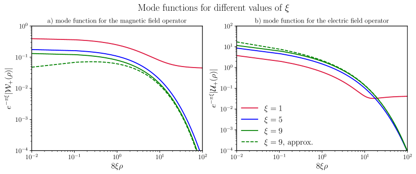
Figure 4: The gauge-field mode functions with positive helicity multiplied by $e^{-\pi\xi}$: (a) $\mathcal{W}_{+}(\rho)$ and (b) $\mathcal{U}_{+}(\rho)$. The red, blue, and green solid curves show the exact mode functions in Eqs. (98)–(102) for $\xi=1$, $5$, and $9$, respectively. The green dashed lines show the approximate mode functions in Eqs. (218)–(219) for $\xi=9$.

With these approximations, the integral in Eq. (114) can be computed analytically. The upper integration limit can be set to infinity since the mode functions in Eqs. (218) and (219) exponentially decay at large arguments and the integral does not diverge in the UV. Keeping only the leading term in the series over the inverse powers of $\xi$, we find the following result:

$$\mathcal{I}(+,p_{\ast};+,p^{\prime}_{\ast};x)=\frac{e^{2\pi\xi}}{\xi^{3}}\frac{15}{128}\frac{x^{4}\big{[}7+Q(p_{\ast},p^{\prime}_{\ast},x)\big{]}}{(p_{\ast}p^{\prime}_{\ast})^{1/4}\big{(}\sqrt{p_{\ast}}+\sqrt{p^{\prime}_{\ast}}\big{)}^{7}}+\mathcal{O}\Big{(}\frac{e^{2\pi\xi}}{\xi^{5}}\Big{)}\,.$$ (221)

Here we have introduced the quantity $Q(p_{\ast},p^{\prime}_{\ast},x)$ defined by

$$Q(p_{\ast},p^{\prime}_{\ast},x)=7h_{1}(+,p_{\ast};+,p^{\prime}_{\ast};x)-4h_{2}(+,p_{\ast};+,p^{\prime}_{\ast};x)=\frac{(p_{\ast}-p^{\prime}_{\ast})^{2}}{x^{2}}$$ (222)

in the case when we take into account the metric perturbations. $Q(p_{\ast},p^{\prime}_{\ast},x)$ is equal to zero if metric perturbations are neglected.

E.2 Scalar power spectrum

Now, let us compute the scalar power spectrum which is parametrized by the function $f_{2}(\xi)$ given by Eq. (118). From Eq. (221), it is obvious that the function $f_{2}(\xi)$ in the limit of large $\xi$ behaves as

$$f_{2}(\xi)=\frac{c_{2}}{\xi^{6}}+\mathcal{O}(\xi^{-8})\,,$$ (223)

and the amplitude $c_{2}$ is given by the integral

$$c_{2}=\frac{15^{2}}{2^{15}\pi}\int d^{3}\bm{p}_{\ast}\sqrt{p_{\ast}|\bm{p}_{\ast}-\hat{\bm{k}}|}\frac{\big{|}\big{(}\bm{\epsilon}_{+}(\bm{p}_{\ast})\cdot\bm{\epsilon}_{+}(\hat{\bm{k}}-\bm{p}_{\ast})\big{)}\big{|}^{2}}{\Big{(}\sqrt{p_{\ast}}+\sqrt{|\bm{p}_{\ast}-\hat{\bm{k}}|}\Big{)}^{14}}\big{[}7+Q(p_{\ast},|\bm{p}_{\ast}-\hat{\bm{k}}|,1)\big{]}^{2}\,,$$ (224)

where $\hat{\bm{k}}=\bm{k}/|\bm{k}|$ and $\bm{p}_{\ast}=\bm{p}/|\bm{k}|$.

Numerically we find

$$c_{2}=\frac{$97\,637$}{$473\,561\,088$}-\frac{195\pi}{$5\,046\,272$}\approx$8.48\text{\times}{10}^{-5}$$$ (225)

for the case when the metric perturbations are included and

$$\tilde{c}_{2}=\frac{172}{$2\,342\,912$}\approx$7.47\text{\times}{10}^{-5}$$$ (226)

for the case where the metric perturbations are neglected (the value reported in Ref. [84]). Thus, taking into account the metric perturbations leads to a change of approximately 12. Note that this difference is only present if one uses the approximate mode functions (218) and (219) for the gauge field. If one takes the exact mode functions instead, both results converge to the same asymptotic value in the limit of large $\xi$, see Fig. 1 and the discussion in the main text.

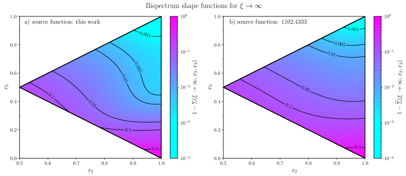
Figure 5: The bispectrum shape function $\Sigma(\xi,x_{2},x_{3})$ in the region of $(x_{2},x_{3})$ plane limited by the inequalities (80) in the large-$\xi$ approximation for the cases when the metric perturbations are (a) included and (b) excluded from the analysis. The latter one coincides with the result of Ref. [84]. Since the shape function exhibits a broad maximum around the equilateral configuration, the color scheme and contour labels corresponds to the deviation of the shape function from unity, $1-\Sigma(\xi,x_{2},x_{3})$, in logarithmic scale.

E.3 Scalar bispectrum

In order to calculate the function $f_{3}(\xi,x_{2},x_{3})$ which describes the scalar bispectrum, we substitute Eq. (221) into Eq. (121). The leading term in the large-$\xi$ expansion has the form

$$f_{3}(\xi,\,x_{2},\,x_{3})=\frac{c_{3}(x_{2},x_{3})}{\xi^{9}}+\mathcal{O}(\xi^{-11})\,,$$ (227)

with

$$c_{3}(x_{2},x_{3}) =-\frac{3^{2}5^{4}}{2^{21}\pi}\frac{x_{2}^{3}x_{3}^{3}}{1+x_{2}^{3}+x_{3}^{3}}\int d^{3}\bm{p}_{\ast}\sqrt{p_{\ast}|\bm{p}_{\ast}-\hat{\bm{k}}_{1}||\hat{\bm{k}}_{3}x_{3}+\bm{p}_{\ast}|}$$

$$\times\frac{\big{(}\bm{\epsilon}_{+}(\bm{p}_{\ast})\cdot\bm{\epsilon}_{+}(\hat{\bm{k}}_{1}-\bm{p}_{\ast})\big{)}\big{(}\bm{\epsilon}_{+}(\bm{p}_{\ast}-\hat{\bm{k}}_{1})\cdot\bm{\epsilon}_{+}(-\hat{\bm{k}}_{3}x_{3}-\bm{p}_{\ast})\big{)}\big{(}\bm{\epsilon}_{+}(\hat{\bm{k}}_{3}x_{3}+\bm{p}_{\ast})\big{)}\cdot\bm{\epsilon}_{+}(-\bm{p}_{\ast})\big{)}}{\Big{(}\sqrt{p_{\ast}}+\sqrt{|\bm{p}_{\ast}-\hat{\bm{k}}_{1}|}\Big{)}^{7}\Big{(}\sqrt{|\hat{\bm{k}}_{3}x_{3}+\bm{p}_{\ast}|}+\sqrt{|\bm{p}_{\ast}-\hat{\bm{k}}_{1}|}\Big{)}^{7}\Big{(}\sqrt{p_{\ast}}+\sqrt{|\hat{\bm{k}}_{3}x_{3}+\bm{p}_{\ast}|}\Big{)}^{7}}$$

$$\times\big{[}7+Q(p_{\ast},|\bm{p}_{\ast}-\hat{\bm{k}}|,1)\big{]}\big{[}7+Q(|\bm{p}_{\ast}-\hat{\bm{k}}|,|\hat{\bm{k}}_{3}x_{3}+\bm{p}_{\ast}|,x_{2})\big{]}\big{[}7+Q(p_{\ast},|\hat{\bm{k}}_{3}x_{3}+\bm{p}_{\ast}|,x_{3})\big{]}\,,$$ (228)

where $\bm{p}_{\ast}=\bm{p}/k$, $\hat{\bm{k}}_{i}=\bm{k}_{i}/|\bm{k}_{i}|$.

In the equilateral configuration $x_{2}=x_{3}=1$, numerically, we obtain

$$c_{3}(1,1)\approx$-3.25\text{\times}{10}^{-7}$\,,$$ (229)

if metric perturbations are included and

$$\tilde{c}_{3}(1,1)\approx$-2.77\text{\times}{10}^{-7}$\,,$$ (230)

when they are neglected which (up to an overall sign) is the same value as reported in Ref. [84]. Again, considering metric perturbations on the same footing with those of the inflaton we obtain a result which is about 15 larger (in the absolute value). Note, however, that in the same manner as for the scalar power spectrum, this difference disappears if one uses the exact gauge-field mode functions instead of the approximate ones, see Fig. 2 in Sec. V.

The bispectrum in nonequilateral momentum configurations is conveniently represented by the shape function $\Sigma$. We show these functions in the large-$\xi$ approximation in Fig. 5 where panel (a) corresponds to the case with metric perturbations included while panel (b) represents the case with the metric perturbations neglected which corresponds to Fig. 6(a) in Ref. [84].

References

- Starobinsky [1980] A. A. Starobinsky, A new type of isotropic cosmological models without singularity, Phys. Lett. B 91, 99 (1980).
- Guth [1981] A. H. Guth, The inflationary universe: A possible solution to the horizon and flatness problems, Phys. Rev. D 23, 347 (1981).
- Linde [1982] A. D. Linde, A new inflationary universe scenario: A possible solution of the horizon, flatness, momogeneity, isotropy and primordial monopole problems, Phys. Lett. B 108, 389 (1982).
- Starobinsky [1982] A. A. Starobinsky, Dynamics of phase transition in the new inflationary universe scenario and generation of perturbations, Phys. Lett. B 117, 175 (1982).
- Albrecht and Steinhardt [1982] A. Albrecht and P. J. Steinhardt, Cosmology for Grand Unified Theories with Radiatively Induced Symmetry Breaking, Phys. Rev. Lett. 48, 1220 (1982).
- Linde [1983] A. D. Linde, Chaotic inflation, Phys. Lett. B 129, 177 (1983).
- Starobinsky [1979] A. A. Starobinsky, Spectrum of relict gravitational radiation and the early state of the universe, JETP Lett. 30, 682 (1979).
- Mukhanov and Chibisov [1981] V. F. Mukhanov and G. V. Chibisov, Quantum fluctuations and a nonsingular universe, JETP Lett. 33, 532 (1981).
- Mukhanov and Chibisov [1982] V. F. Mukhanov and G. V. Chibisov, Vacuum energy and large scale structure of the Universe, Sov. Phys. JETP 56, 258 (1982).
- Guth and Pi [1982] A. H. Guth and S. Y. Pi, Fluctuations in the New Inflationary Universe, Phys. Rev. Lett. 49, 1110 (1982).
- Hawking [1982] S. W. Hawking, The development of irregularities in a single bubble inflationary universe, Phys. Lett. B 115, 295 (1982).
- Bardeen et al. [1983] J. M. Bardeen, P. J. Steinhardt, and M. S. Turner, Spontaneous creation of almost scale-free density perturbations in an inflationary universe, Phys. Rev. D 28, 679 (1983).
- Ade et al. [2014] P. A. R. Ade et al. (Planck), Planck 2013 results. XXII. Constraints on inflation, Astron. Astrophys. 571, A22 (2014), arXiv:1303.5082 [astro-ph.CO] .
- Ade et al. [2016a] P. A. R. Ade et al. (Planck), Planck 2015 results. XX. Constraints on inflation, Astron. Astrophys. 594, A20 (2016a), arXiv:1502.02114 [astro-ph.CO] .
- Akrami et al. [2020a] Y. Akrami et al. (Planck), Planck 2018 results. X. Constraints on inflation, Astron. Astrophys. 641, A10 (2020a), arXiv:1807.06211 [astro-ph.CO] .
- Reid et al. [2010] B. A. Reid et al., Cosmological constraints from the clustering of the Sloan Digital Sky Survey DR7 luminous red galaxies, Mon. Not. Roy. Astron. Soc. 404, 60 (2010), arXiv:0907.1659 [astro-ph.CO] .
- Cabass et al. [2022] G. Cabass, M. M. Ivanov, O. H. E. Philcox, M. Simonović, and M. Zaldarriaga, Constraints on Single-Field Inflation from the BOSS Galaxy Survey, Phys. Rev. Lett. 129, 021301 (2022), arXiv:2201.07238 [astro-ph.CO] .
- Martin et al. [2014] J. Martin, C. Ringeval, and V. Vennin, Encyclopædia inflationaris, Phys. Dark Univ. 5–6, 75 (2014), arXiv:1303.3787 [astro-ph.CO] .
- Chluba et al. [2015] J. Chluba, J. Hamann, and S. P. Patil, Features and new physical scales in primordial observables: Theory and observation, Int. J. Mod. Phys. D 24, 1530023 (2015), arXiv:1505.01834 [astro-ph.CO] .
- Martin [2020] J. Martin, The theory of inflation, Proc. Int. Sch. Phys. Fermi 200, 155 (2020), arXiv:1807.11075 [astro-ph.CO] .
- Durrer [2020] R. Durrer, The Cosmic Microwave Background (Cambridge University Press, Cambridge, 2020).
- [22] J. Martin, C. Ringeval, and V. Vennin, Cosmic inflation at the crossroads, arXiv:2404.10647 [astro-ph.CO] .
- Bartolo et al. [2004] N. Bartolo, E. Komatsu, S. Matarrese, and A. Riotto, Non-Gaussianity from inflation: Theory and observations, Phys. Rept. 402, 103 (2004), arXiv:astro-ph/0406398 .
- Ade et al. [2016b] P. A. R. Ade et al. (Planck), Planck 2015 results: XVII. Constraints on primordial non-Gaussianity, Astron. Astrophys. 594, A17 (2016b), arXiv:1502.01592 [astro-ph.CO] .
- Akrami et al. [2020b] Y. Akrami et al. (Planck), Planck 2018 results: IX. Constraints on primordial non-Gaussianity, Astron. Astrophys. 641, A9 (2020b), arXiv:1905.05697 [astro-ph.CO] .
- Kronberg [1994] P. P. Kronberg, Extragalactic magnetic fields, Rept. Prog. Phys. 57, 325 (1994).
- Ryu et al. [2012] D. Ryu, D. R. G. Schleicher, R. A. Treumann, C. G. Tsagas, and L. M. Widrow, Magnetic fields in the large-scale structure of the Universe, Space Sci. Rev. 166, 1 (2012), arXiv:1109.4055 [astro-ph.CO] .
- Vallee [2011] J. P. Vallee, Magnetic fields in the galactic Universe, as observed in supershells, galaxies, intergalactic and cosmic realms, New Astron. Rev. 55, 91 (2011).
- Vachaspati [2021] T. Vachaspati, Progress on cosmological magnetic fields, Rept. Prog. Phys. 84, 074901 (2021), arXiv:2010.10525 [astro-ph.CO] .
- Bernet et al. [2008] M. L. Bernet, F. Miniati, S. J. Lilly, P. P. Kronberg, and M. Dessauges-Zavadsky, Strong magnetic fields in normal galaxies at high redshifts, Nature 454, 302 (2008), arXiv:0807.3347 [astro-ph] .
- Bonafede et al. [2010] A. Bonafede, L. Feretti, M. Murgia, F. Govoni, G. Giovannini, and V. Vacca, Galaxy cluster magnetic fields from radio polarized emission, PoS ISKAF2010, 006 (2010), arXiv:1009.1233 [astro-ph.CO] .
- Feretti et al. [2012] L. Feretti, G. Giovannini, F. Govoni, and M. Murgia, Clusters of galaxies: Observational properties of the diffuse radio emission, Astron. Astrophys. Rev. 20, 54 (2012), arXiv:1205.1919 [astro-ph.CO] .
- Vacca et al. [2018] V. Vacca et al., Observations of a nearby filament of galaxy clusters with the Sardinia Radio Telescope, Mon. Not. Roy. Astron. Soc. 479, 776 (2018), arXiv:1804.09199 [astro-ph.CO] .
- Carretti et al. [2022] E. Carretti, S. P. O’Sullivan, V. Vacca, F. Vazza, C. Gheller, T. Vernstrom, and A. Bonafede, Magnetic field evolution in cosmic filaments with LOFAR data, Mon. Not. Roy. Astron. Soc. 518, 2273 (2022), arXiv:2210.06220 [astro-ph.CO] .
- Neronov and Vovk [2010] A. Neronov and I. Vovk, Evidence for strong extragalactic magnetic fields from Fermi observations of TeV blazars, Science 328, 73 (2010), arXiv:1006.3504 [astro-ph.HE] .
- Tavecchio et al. [2011] F. Tavecchio, G. Ghisellini, G. Bonnoli, and L. Foschini, Extreme TeV blazars and the intergalactic magnetic field, Mon. Not. Roy. Astron. Soc. 414, 3566 (2011), arXiv:1009.1048 [astro-ph.HE] .
- Tavecchio et al. [2010] F. Tavecchio, G. Ghisellini, L. Foschini, G. Bonnoli, G. Ghirlanda, and P. Coppi, The intergalactic magnetic field constrained by Fermi/LAT observations of the TeV blazar 1ES 0229+200, Mon. Not. Roy. Astron. Soc. 406, L70 (2010), arXiv:1004.1329 [astro-ph.CO] .
- Ando and Kusenko [2010] S. Ando and A. Kusenko, Evidence for gamma-ray halos around active galactic nuclei and the first measurement of intergalactic magnetic fields, Astrophys. J. Lett. 722, L39 (2010), arXiv:1005.1924 [astro-ph.HE] .
- Dermer et al. [2011] C. D. Dermer, M. Cavadini, S. Razzaque, J. D. Finke, J. Chiang, and B. Lott, Time delay of cascade radiation for TeV blazars and the measurement of the intergalactic magnetic field, Astrophys. J. Lett. 733, L21 (2011), arXiv:1011.6660 [astro-ph.HE] .
- Dolag et al. [2011] K. Dolag, M. Kachelriess, S. Ostapchenko, and R. Tomas, Lower limit on the strength and filling factor of extragalactic magnetic fields, Astrophys. J. Lett. 727, L4 (2011), arXiv:1009.1782 [astro-ph.HE] .
- Vovk et al. [2012] I. Vovk, A. M. Taylor, D. Semikoz, and A. Neronov, Fermi/LAT observations of 1ES 0229+200: Implications for extragalactic magnetic fields and background light, Astrophys. J. Lett. 747, L14 (2012), arXiv:1112.2534 [astro-ph.CO] .
- Huan et al. [2011] H. Huan, T. Weisgarber, T. Arlen, and S. P. Wakely, A new model for gamma-ray cascades in extragalactic magnetic fields, Astrophys. J. Lett. 735, L28 (2011), arXiv:1106.1218 [astro-ph.HE] .
- Taylor et al. [2011] A. M. Taylor, I. Vovk, and A. Neronov, Extragalactic magnetic fields constraints from simultaneous GeV-TeV observations of blazars, Astron. Astrophys. 529, A144 (2011), arXiv:1101.0932 [astro-ph.HE] .
- Neronov et al. [2013] A. Neronov, A. M. Taylor, C. Tchernin, and I. Vovk, Measuring the correlation length of intergalactic magnetic fields from observations of gamma-ray induced cascades, Astron. Astrophys. 554, A31 (2013), arXiv:1307.2753 [astro-ph.HE] .
- Caprini and Gabici [2015] C. Caprini and S. Gabici, Gamma-ray observations of blazars and the intergalactic magnetic field spectrum, Phys. Rev. D 91, 123514 (2015), arXiv:1504.00383 [astro-ph.CO] .
- Alves Batista and Saveliev [2020] R. Alves Batista and A. Saveliev, Multimessenger constraints on intergalactic magnetic fields from the flare of TXS 0506+056, Astrophys. J. Lett. 902, L11 (2020), arXiv:2009.12161 [astro-ph.HE] .
- Alves Batista and Saveliev [2021] R. Alves Batista and A. Saveliev, The gamma-ray window to intergalactic magnetism, Universe 7, 223 (2021), arXiv:2105.12020 [astro-ph.HE] .
- Acciari et al. [2023] V. A. Acciari et al. (MAGIC), A lower bound on intergalactic magnetic fields from time variability of 1ES 0229+200 from MAGIC and Fermi/LAT observations, Astron. Astrophys. 670, A145 (2023), arXiv:2210.03321 [astro-ph.HE] .
- Tjemsland et al. [2024] J. Tjemsland, M. Meyer, and F. Vazza, Constraining the astrophysical origin of intergalactic magnetic fields, Astrophys. J. 963, 135 (2024), arXiv:2311.04273 [astro-ph.HE] .
- Parker [1968] L. Parker, Particle Creation in Expanding Universes, Phys. Rev. Lett. 21, 562 (1968).
- Turner and Widrow [1988] M. S. Turner and L. M. Widrow, Inflation produced, large scale magnetic fields, Phys. Rev. D 37, 2743 (1988).
- Ratra [1992] B. Ratra, Cosmological ‘seed’ magnetic field from inflation, Astrophys. J. Lett. 391, L1 (1992).
- Garretson et al. [1992] W. D. Garretson, G. B. Field, and S. M. Carroll, Primordial magnetic fields from pseudo Goldstone bosons, Phys. Rev. D 46, 5346 (1992), arXiv:hep-ph/9209238 .
- Martin and Yokoyama [2008] J. Martin and J. Yokoyama, Generation of large-scale magnetic fields in single-field inflation, J. Cosmol. Astropart. Phys. 01 (2008) 025, arXiv:0711.4307 [astro-ph] .
- Anber and Sorbo [2006] M. M. Anber and L. Sorbo, N-lationary magnetic fields, J. Cosmol. Astropart. Phys. 10 (2006) 018, arXiv:astro-ph/0606534 .
- Giovannini [2004] M. Giovannini, The magnetized Universe, Int. J. Mod. Phys. D 13, 391 (2004), arXiv:astro-ph/0312614 .
- Subramanian [2010] K. Subramanian, Magnetic fields in the early Universe, Astron. Nachr. 331, 110 (2010), arXiv:0911.4771 [astro-ph.CO] .
- Kandus et al. [2011] A. Kandus, K. E. Kunze, and C. G. Tsagas, Primordial magnetogenesis, Phys. Rept. 505, 1 (2011), arXiv:1007.3891 [astro-ph.CO] .
- Durrer and Neronov [2013] R. Durrer and A. Neronov, Cosmological magnetic fields: Their generation, evolution and observation, Astron. Astrophys. Rev. 21, 62 (2013), arXiv:1303.7121 [astro-ph.CO] .
- Subramanian [2016] K. Subramanian, The origin, evolution and signatures of primordial magnetic fields, Rept. Prog. Phys. 79, 076901 (2016), arXiv:1504.02311 [astro-ph.CO] .
- Seery [2009] D. Seery, Magnetogenesis and the primordial non-Gaussianity, J. Cosmol. Astropart. Phys. 08 (2009) 018, arXiv:0810.1617 [astro-ph] .
- Yokoyama and Soda [2008] S. Yokoyama and J. Soda, Primordial statistical anisotropy generated at the end of inflation, J. Cosmol. Astropart. Phys. 08 (2008) 005, arXiv:0805.4265 [astro-ph] .
- Dimastrogiovanni et al. [2010] E. Dimastrogiovanni, N. Bartolo, S. Matarrese, and A. Riotto, Non-Gaussianity and Statistical Anisotropy from Vector Field Populated Inflationary Models, Adv. Astron. 2010, 752670 (2010), arXiv:1001.4049 [astro-ph.CO] .
- Watanabe et al. [2010] M.-a. Watanabe, S. Kanno, and J. Soda, The Nature of Primordial Fluctuations from Anisotropic Inflation, Prog. Theor. Phys. 123, 1041 (2010), arXiv:1003.0056 [astro-ph.CO] .
- Caldwell et al. [2011] R. R. Caldwell, L. Motta, and M. Kamionkowski, Correlation of inflation-produced magnetic fields with scalar fluctuations, Phys. Rev. D 84, 123525 (2011), arXiv:1109.4415 [astro-ph.CO] .
- Bonvin et al. [2012] C. Bonvin, C. Caprini, and R. Durrer, Magnetic fields from inflation: The transition to the radiation era, Phys. Rev. D 86, 023519 (2012), arXiv:1112.3901 [astro-ph.CO] .
- Bartolo et al. [2013] N. Bartolo, S. Matarrese, M. Peloso, and A. Ricciardone, Anisotropic power spectrum and bispectrum in the mechanism, Phys. Rev. D 87, 023504 (2013), arXiv:1210.3257 [astro-ph.CO] .
- Motta and Caldwell [2012] L. Motta and R. R. Caldwell, Non-Gaussian features of primordial magnetic fields in power-law inflation, Phys. Rev. D 85, 103532 (2012), arXiv:1203.1033 [astro-ph.CO] .
- Jain and Sloth [2012] R. K. Jain and M. S. Sloth, Consistency relation for cosmic magnetic fields, Phys. Rev. D 86, 123528 (2012), arXiv:1207.4187 [astro-ph.CO] .
- Jain and Sloth [2013] R. K. Jain and M. S. Sloth, On the non-Gaussian correlation of the primordial curvature perturbation with vector fields, J. Cosmol. Astropart. Phys. 02 (2013) 003, arXiv:1210.3461 [astro-ph.CO] .
- Shiraishi et al. [2012] M. Shiraishi, S. Saga, and S. Yokoyama, CMB power spectra induced by primordial cross-bispectra between metric perturbations and vector fields, J. Cosmol. Astropart. Phys. 11 (2012) 046, arXiv:1209.3384 [astro-ph.CO] .
- Soda [2012] J. Soda, Statistical anisotropy from anisotropic inflation, Class. Quant. Grav. 29, 083001 (2012), arXiv:1201.6434 [hep-th] .
- Suyama and Yokoyama [2012] T. Suyama and J. Yokoyama, Metric perturbation from an inflationary magnetic field and a generic bound on inflation models, Phys. Rev. D 86, 023512 (2012), arXiv:1204.3976 [astro-ph.CO] .
- Abolhasani et al. [2013] A. A. Abolhasani, R. Emami, J. T. Firouzjaee, and H. Firouzjahi, formalism in anisotropic inflation and large anisotropic bispectrum and trispectrum, J. Cosmol. Astropart. Phys. 08 (2013) 016, arXiv:1302.6986 [astro-ph.CO] .
- Nurmi and Sloth [2014] S. Nurmi and M. S. Sloth, Constraints on gauge field production during inflation, J. Cosmol. Astropart. Phys. 07 (2014) 012, arXiv:1312.4946 [astro-ph.CO] .
- Thorsrud et al. [2014] M. Thorsrud, F. R. Urban, and D. F. Mota, Statistics of anisotropies in inflation with spectator vector fields, J. Cosmol. Astropart. Phys. 04 (2014) 010, arXiv:1312.7491 [astro-ph.CO] .
- Giovannini [2013] M. Giovannini, Fluctuations of inflationary magnetogenesis, Phys. Rev. D 87, 083004 (2013), arXiv:1302.2243 [hep-th] .
- Fujita and Yokoyama [2013] T. Fujita and S. Yokoyama, Higher order statistics of curvature perturbations in model and its Planck constraints, J. Cosmol. Astropart. Phys. 09 (2013) 009, arXiv:1306.2992 [astro-ph.CO] .
- Choi et al. [2015] K. Choi, K.-Y. Choi, H. Kim, and C. S. Shin, Primordial perturbations from dilaton-induced gauge fields, J. Cosmol. Astropart. Phys. 10 (2015) 046, arXiv:1507.04977 [astro-ph.CO] .
- Chua et al. [2019] W. Z. Chua, Q. Ding, Y. Wang, and S. Zhou, Imprints of Schwinger effect on primordial spectra, J. High Energy Phys. 04 (2019) 066, arXiv:1810.09815 [hep-th] .
- [81] C.-B. Chen, Inflation with vector fields revisited: Heavy entropy perturbations and primordial black holes, arXiv:2312.06105 [astro-ph.CO] .
- Anber and Sorbo [2010] M. M. Anber and L. Sorbo, Naturally inflating on steep potentials through electromagnetic dissipation, Phys. Rev. D 81, 043534 (2010), arXiv:0908.4089 [hep-th] .
- Barnaby and Peloso [2011] N. Barnaby and M. Peloso, Large Non-Gaussianity in Axion Inflation, Phys. Rev. Lett. 106, 181301 (2011), arXiv:1011.1500 [hep-ph] .
- Barnaby et al. [2011] N. Barnaby, R. Namba, and M. Peloso, Phenomenology of a pseudo-scalar inflaton: naturally large nongaussianity, J. Cosmol. Astropart. Phys. 04 (2011) 009, arXiv:1102.4333 [astro-ph.CO] .
- Barnaby et al. [2012a] N. Barnaby, E. Pajer, and M. Peloso, Gauge field production in axion inflation: Consequences for monodromy, non-Gaussianity in the CMB, and gravitational waves at interferometers, Phys. Rev. D 85, 023525 (2012a), arXiv:1110.3327 [astro-ph.CO] .
- Barnaby et al. [2012b] N. Barnaby, J. Moxon, R. Namba, M. Peloso, G. Shiu, and P. Zhou, Gravity waves and non-Gaussian features from particle production in a sector gravitationally coupled to the inflaton, Phys. Rev. D 86, 103508 (2012b), arXiv:1206.6117 [astro-ph.CO] .
- Linde et al. [2013] A. Linde, S. Mooij, and E. Pajer, Gauge field production in supergravity inflation: Local non-Gaussianity and primordial black holes, Phys. Rev. D 87, 103506 (2013), arXiv:1212.1693 [hep-th] .
- Meerburg and Pajer [2013] P. D. Meerburg and E. Pajer, Observational constraints on gauge field production in axion inflation, J. Cosmol. Astropart. Phys. 02 (2013) 017, arXiv:1203.6076 [astro-ph.CO] .
- Bamba [2015] K. Bamba, Generation of large-scale magnetic fields, non-Gaussianity, and primordial gravitational waves in onflationary cosmology, Phys. Rev. D 91, 043509 (2015), arXiv:1411.4335 [astro-ph.CO] .
- Fujita et al. [2015] T. Fujita, R. Namba, Y. Tada, N. Takeda, and H. Tashiro, Consistent generation of magnetic fields in axion inflation models, J. Cosmol. Astropart. Phys. 05 (2015) 054, arXiv:1503.05802 [astro-ph.CO] .
- Namba et al. [2016] R. Namba, M. Peloso, M. Shiraishi, L. Sorbo, and C. Unal, Scale-dependent gravitational waves from a rolling axion, J. Cosmol. Astropart. Phys. 01 (2016) 041, arXiv:1509.07521 [astro-ph.CO] .
- Dimastrogiovanni et al. [2017] E. Dimastrogiovanni, M. Fasiello, and T. Fujita, Primordial gravitational waves from axion–gauge fields dynamics, J. Cosmol. Astropart. Phys. 01 (2017) 019, arXiv:1608.04216 [astro-ph.CO] .
- Domcke et al. [2016] V. Domcke, M. Pieroni, and P. Binétruy, Primordial gravitational waves for universality classes of pseudoscalar inflation, J. Cosmol. Astropart. Phys. 06 (2016) 031, arXiv:1603.01287 [astro-ph.CO] .
- García-Bellido et al. [2016] J. García-Bellido, M. Peloso, and C. Unal, Gravitational waves at interferometer scales and primordial black holes in axion inflation, J. Cosmol. Astropart. Phys. 12 (2016) 031, arXiv:1610.03763 [astro-ph.CO] .
- Papageorgiou et al. [2018] A. Papageorgiou, M. Peloso, and C. Unal, Nonlinear perturbations from the coupling of the inflaton to a non-Abelian gauge field, with a focus on Chromo-Natural Inflation, J. Cosmol. Astropart. Phys. 09 (2018) 030, arXiv:1806.08313 [astro-ph.CO] .
- Papageorgiou et al. [2019] A. Papageorgiou, M. Peloso, and C. Unal, Nonlinear perturbations from axion–gauge fields dynamics during inflation, J. Cosmol. Astropart. Phys. 07 (2019) 004, arXiv:1904.01488 [astro-ph.CO] .
- Domcke et al. [2020] V. Domcke, V. Guidetti, Y. Welling, and A. Westphal, Resonant backreaction in axion inflation, J. Cosmol. Astropart. Phys. 09 (2020) 009, arXiv:2002.02952 [astro-ph.CO] .
- Dimastrogiovanni et al. [2024] E. Dimastrogiovanni, M. Fasiello, M. Michelotti, and L. Pinol, Primordial gravitational waves in non-minimally coupled chromo-natural inflation, J. Cosmol. Astropart. Phys. 02 (2024) 039, arXiv:2303.10718 [astro-ph.CO] .
- Domcke et al. [2024] V. Domcke, Y. Ema, and S. Sandner, Perturbatively including inhomogeneities in axion inflation, J. Cosmol. Astropart. Phys. 03 (2024) 019, arXiv:2310.09186 [astro-ph.CO] .
- [100] S. P. Corbà and L. Sorbo, Correlated scalar perturbations and gravitational waves from axion inflation, arXiv:2403.03338 [astro-ph.CO] .
- Valenzuela-Toledo and Rodríguez [2010] C. A. Valenzuela-Toledo and Y. Rodríguez, Non-Gaussianity from the trispectrum and vector field perturbations, Phys. Lett. B 685, 120 (2010), arXiv:0910.4208 [astro-ph.CO] .
- Ringeval et al. [2013] C. Ringeval, T. Suyama, and J. Yokoyama, Magneto-reheating constraints from curvature perturbations, J. Cosmol. Astropart. Phys. 09 (2013) 020, arXiv:1302.6013 [astro-ph.CO] .
- Fujita and Yokoyama [2014] T. Fujita and S. Yokoyama, Critical constraint on inflationary magnetogenesis, J. Cosmol. Astropart. Phys. 03 (2014) 013, arXiv:1402.0596 [astro-ph.CO] .
- Kamada et al. [2021] K. Kamada, F. Uchida, and J. Yokoyama, Baryon isocurvature constraints on the primordial hypermagnetic fields, J. Cosmol. Astropart. Phys. 04 (2021) 034, arXiv:2012.14435 [astro-ph.CO] .
- Deskins et al. [2013] J. T. Deskins, J. T. Giblin, and R. R. Caldwell, Gauge field preheating at the end of inflation, Phys. Rev. D 88, 063530 (2013), arXiv:1305.7226 [astro-ph.CO] .
- Caravano et al. [2023] A. Caravano, E. Komatsu, K. D. Lozanov, and J. Weller, Lattice simulations of axion-U(1) inflation, Phys. Rev. D 108, 043504 (2023), arXiv:2204.12874 [astro-ph.CO] .
- Figueroa et al. [2023] D. G. Figueroa, J. Lizarraga, A. Urio, and J. Urrestilla, The Strong Backreaction Regime in Axion Inflation, Phys. Rev. Lett. 131, 151003 (2023), arXiv:2303.17436 [astro-ph.CO] .
- Durrer et al. [2023] R. Durrer, O. Sobol, and S. Vilchinskii, Backreaction from gauge fields produced during inflation, Phys. Rev. D 108, 043540 (2023), arXiv:2303.04583 [gr-qc] .
- Gorbar et al. [2021] E. V. Gorbar, K. Schmitz, O. O. Sobol, and S. I. Vilchinskii, Gauge-field production during axion inflation in the gradient expansion formalism, Phys. Rev. D 104, 123504 (2021), arXiv:2109.01651 [hep-ph] .
- von Eckardstein et al. [2023] R. von Eckardstein, M. Peloso, K. Schmitz, O. Sobol, and L. Sorbo, Axion inflation in the strong-backreaction regime: Decay of the Anber-Sorbo solution, J. High Energy Phys. 11 (2023) 183, arXiv:2309.04254 [hep-ph] .
- Durrer [1990] R. Durrer, Gauge invariant cosmological perturbation theory with seeds, Phys. Rev. D 42, 2533 (1990).
- Durrer [1994] R. Durrer, Gauge invariant cosmological perturbation theory: A general study and its application to the texture scenario of structure formation, Fund. Cosmic Phys. 15, 209 (1994), arXiv:astro-ph/9311041 .
- Jordan and Pauli [1928] P. Jordan and W. Pauli, Zur Quantenelektrodynamik ladungsfreier Felder (On the quantum electrodynamics of charge-free fields), Z. Phys. 47, 151 (1928).
- Heisenberg and Pauli [1929] W. Heisenberg and W. Pauli, Zur Quantendynamik der Wellenfelder (On the quantum dynamics of wave fields), Z. Phys. 56, 1 (1929).
- Bohr and Rosenfeld [1933] N. Bohr and L. Rosenfeld, Zur Frage der Messbarkeit der elektromagnetischen Feldgrössen (On the question of the measurability of electromagnetic field variables), K. Dan. Vidensk. Selsk. Mat.-Fys. Medd. 12, 1 (1933).
- Stewart [2011] A. Stewart, Quantisation of the free electromagnetic field implies quantisation of its angular momentum, J. Mod. Opt. 58, 772 (2011), arXiv:1011.4131 [math-ph] .
- Sobol et al. [2019] O. O. Sobol, E. V. Gorbar, and S. I. Vilchinskii, Backreaction of electromagnetic fields and the Schwinger effect in pseudoscalar inflation magnetogenesis, Phys. Rev. D 100, 063523 (2019), arXiv:1907.10443 [astro-ph.CO] .
- Sobol et al. [2020] O. O. Sobol, A. V. Lysenko, E. V. Gorbar, and S. I. Vilchinskii, Gradient expansion formalism for magnetogenesis in the kinetic coupling model, Phys. Rev. D 102, 123512 (2020), arXiv:2010.13587 [astro-ph.CO] .
- Nakamura and Stewart [1996] T. T. Nakamura and E. D. Stewart, The spectrum of cosmological perturbations produced by a multi-component inflaton to second order in the slow-roll approximation, Phys. Lett. B 381, 413 (1996), arXiv:astro-ph/9604103 .
- Gordon et al. [2000] C. Gordon, D. Wands, B. A. Bassett, and R. Maartens, Adiabatic and entropy perturbations from inflation, Phys. Rev. D 63, 023506 (2000), arXiv:astro-ph/0009131 .
- Gong and Tanaka [2011] J.-O. Gong and T. Tanaka, A covariant approach to general field space metric in multi-field inflation, J. Cosmol. Astropart. Phys. 03 (2011) 015, arXiv:1101.4809 [astro-ph.CO] .
- Gangui et al. [1994] A. Gangui, F. Lucchin, S. Matarrese, and S. Mollerach, The three-point correlation function of the cosmic microwave background in inflationary models, Astrophys. J. 430, 447 (1994), arXiv:astro-ph/9312033 .
- Acquaviva et al. [2003] V. Acquaviva, N. Bartolo, S. Matarrese, and A. Riotto, Gauge-invariant second-order perturbations and non-Gaussianity from inflation, Nucl. Phys. B 667, 119 (2003), arXiv:astro-ph/0209156 .
- Maldacena [2003] J. Maldacena, Non-Gaussian features of primordial fluctuations in single field inflationary models, J. High Energy Phys. 05 (2003) 013, arXiv:astro-ph/0210603 .
- Babich et al. [2004] D. Babich, P. Creminelli, and M. Zaldarriaga, The shape of non-Gaussianities, J. Cosmol. Astropart. Phys. 08 (2004) 009, arXiv:astro-ph/0405356 .
- Fergusson and Shellard [2009] J. R. Fergusson and E. P. S. Shellard, Shape of primordial non-Gaussianity and the CMB bispectrum, Phys. Rev. D 80, 043510 (2009), arXiv:0812.3413 [astro-ph] .
- Komatsu and Spergel [2001] E. Komatsu and D. N. Spergel, Acoustic signatures in the primary microwave background bispectrum, Phys. Rev. D 63, 063002 (2001), arXiv:astro-ph/0005036 .
- Creminelli et al. [2006] P. Creminelli, A. Nicolis, L. Senatore, M. Tegmark, and M. Zaldarriaga, Limits on non-Gaussianities from WMAP data, J. Cosmol. Astropart. Phys. 05 (2006) 004, arXiv:astro-ph/0509029 .
- Senatore et al. [2010] L. Senatore, K. M. Smith, and M. Zaldarriaga, Non-Gaussianities in single field inflation and their optimal limits from the WMAP 5-year data, J. Cosmol. Astropart. Phys. 01 (2010) 028, arXiv:0905.3746 [astro-ph.CO] .
- Abramowitz and Stegun [1972] M. Abramowitz and I. Stegun, eds., Handbook of Mathematical Functions with Formulas, Graphs, and Mathematical Tables, National Bureau of Standards Applied Mathematics Series, Vol. 55 (U.S. Government Printing Office, Washington, D.C., 1972) 10th printing, with corrections.
- Durrer et al. [2011] R. Durrer, L. Hollenstein, and R. K. Jain, Can slow roll inflation induce relevant helical magnetic fields?, J. Cosmol. Astropart. Phys. 03 (2011) 037, arXiv:1005.5322 [astro-ph.CO] .
- Jiménez et al. [2017] D. Jiménez, K. Kamada, K. Schmitz, and X.-J. Xu, Baryon asymmetry and gravitational waves from pseudoscalar inflation, J. Cosmol. Astropart. Phys. 12 (2017) 011, arXiv:1707.07943 [hep-ph] .
- Peloso and Sorbo [2023] M. Peloso and L. Sorbo, Instability in axion inflation with strong backreaction from gauge modes, J. Cosmol. Astropart. Phys. 01 (2023) 038, arXiv:2209.08131 [astro-ph.CO] .
- Ballardini et al. [2019] M. Ballardini, M. Braglia, F. Finelli, G. Marozzi, and A. A. Starobinsky, Energy-momentum tensor and helicity for gauge fields coupled to a pseudo-scalar inflaton, Phys. Rev. D 100, 123542 (2019), arXiv:1910.13448 [gr-qc] .
- Domcke and Mukaida [2018] V. Domcke and K. Mukaida, Gauge field and fermion production during axion inflation, J. Cosmol. Astropart. Phys. 11 (2018) 020, arXiv:1806.08769 [hep-ph] .
- García-Bellido et al. [2024] J. García-Bellido, A. Papageorgiou, M. Peloso, and L. Sorbo, A flashing beacon in axion inflation: Recurring bursts of gravitational waves in the strong backreaction regime, J. Cosmol. Astropart. Phys. 01 (2024) 034, arXiv:2303.13425 [astro-ph.CO] .