Supplemental Material for:
The finite-$T$ Lorentz number and the thermal conductivity.
Aluminum and carbon conductivities from ambient to millions of degrees Kelvin

Abstract

This supplemental material (SM) covers the following topics:
(i) Derivation of the finite-$T$ form of the Lorentz number $L_{n}(t)$
(ii) Electron-electron interactions in DFT and in conventional approaches.
(iii) The electrical conductivity from Pseudopotentials and from the T-matrix form of the scattering cross section.
(iv) Results for $l$-Al at 2.7 g/cm³, $l$-carbon at 10 g/cm³, and at the “diamond-like” density of 3.6 g/cm³.

I Derivation of the finite-$T$ form of the Lorentz number

We use Hartree atomic units, with $\hbar=m_{e}=|e|=1$, and $T$ such that the Boltzmann constant $k_{B}=1$. The symbols defined in the main text are also used in this supplemental material without further definition unless additional clarification is needed.

In the following we use the following normalization of the Fermi function:

$$\bar{n} = \int\frac{d\vec{k}}{4\pi^{3}}f(k)$$ (1)

$$f(k) = f(\epsilon)=1/\left[1+\exp(\epsilon-\mu)/T\right]$$ (2)

$$\epsilon = k^{2}/2.$$ (3)

Then the classical limit is given by

$$f(e) = \exp(\mu/T)\exp(-\epsilon/T)$$ (4)

$$e^{(\mu/T)} = \frac{\bar{n}}{2}\left[\frac{2\pi}{T}\right]^{3/2}.$$ (5)

The above normalization is commonly used AshMer76 , but differs from the usage in some standard texts LLvol10 . Furthermore, in the NPA, the volume occupied by the free electrons is not the ionic Wigner-Seitz sphere of radius $r_{ws}=\{3/4\pi\bar{\rho}\}^{1/3}$, but an infinitely large volume, approximated by a volume of radius $R_{c}$ of the “correlation sphere” of the fluid. It is such that, given a nucleus placed at the origin of the correlation sphere, all pair-distribution functions $g_{ss^{\prime}}(r)$, where the species $s$ or $s^{\prime}$ may be electrons or ions, have decayed to unity when $r\to R_{c}$. For $T<E_{F}$, usually $R_{c}\sim 10r_{ws}$, while for higher $T$ we have used $R_{c}\sim 5r_{ws}$.

The non-interacting electrons (i.e., Kohn-Sham electrons) populating the correlation sphere take the noninteracting value $\mu^{0}$ for its chemical potential, as required by DFT. This model is discussed in more detail in Refs. DWP82 ; eos95 . Average-atom models that confine the free electrons to within the ionic Wigner-Seitz sphere become similar to our NPA model for $T$ sufficiently large, such that $g_{ie}(r)=n(r)/\bar{n}$ has already decayed to unity as $r\to r_{ws}$.

We define the kinetic coefficients $\mathcal{L}^{\alpha}$ as in Ashcroft and Mermin, Chapter 13 AshMer76 . We use the notation $\langle\cdots\rangle$ used in the main text to indicate averaging over $-df(\epsilon)/d\epsilon$. Then,

$$\mathcal{L}^{\alpha} = \langle(\epsilon-\mu)^{\alpha}\tau(\epsilon)I(\epsilon)\rangle$$ (6)

$$I(\epsilon) = \int\frac{d\vec{k}}{4\pi^{3}}\delta(\epsilon-\epsilon(\vec{k}))\vec{V}_{\vec{k}}\vec{V}_{\vec{k}}.$$ (7)

As we are considering a uniform fluid with $\epsilon(\vec{k})=k^{2}/2$, $\vec{V}\vec{V}=(1/3)V^{2}$, the above equation can be written as:

$$\mathcal{L}^{\alpha} = C_{0}\langle(\epsilon-\mu)^{\alpha}\epsilon^{3/2}\tau_{ei}(\epsilon)\rangle$$ (8)

$$C_{0} = \frac{2\surd{2}}{3\pi^{2}}$$ (9)

A generic form for $\tau_{ei}(\epsilon)$ can be obtained from the Rutherford formula for the scattering of an electron by a heavy ion of charge $\bar{Z}$. This leads to the Landau-Spitzer form if written in terms of a Coulomb Logarithm $C_{lg}$ (see Sec 44, of  LLvol10 ). Here we have restored the constants $m_{e}$ and $e$ for clarity.

$$\tau_{ei}(\epsilon) = \frac{m_{e}^{1/2}(2\epsilon)^{3/2}}{4\pi Ze^{4}\bar{n}C_{lg}}$$ (10)

$$= C_{ei}\epsilon^{3/2}$$ (11)

A more sophisticated calculation of the scattering, inclusive of the ion-distribution by including a structure factor, pseudopotentials or a T-matrix usually amounts to an improved form for $C_{lg}$. Our main purpose here is to provide a tractable form for $\tau_{ei}(\epsilon)$ to evaluate the kinetic coefficients analytically, and the analysis remains valid as long as any improved from for $C_{lg}$ does not introduce any additional dependence on $\epsilon$. Then, for $T>0$, the $df/d\epsilon$ can be reduced by a partial integration to give:

$$\mathcal{L}^{(0)} = C_{1}\int d\epsilon f(\epsilon)3\epsilon^{2},\;C_{1}=C_{0}C_{ei}$$ (12)

$$\mathcal{L}^{(1)} = C_{1}\int d\epsilon f(\epsilon)(4\epsilon^{3}-3\mu\epsilon^{2})$$ (13)

$$\mathcal{L}^{(2)} = C_{1}\int d\epsilon f(\epsilon)(5\epsilon^{4}-8\mu\epsilon^{3}+3\mu^{2}\epsilon^{2})$$ (14)

These results can be incorporated into the expression for the Lorentz number $L_{N}$.

$$L_{N} = \frac{1}{T^{2}}\left[\frac{\mathcal{L}^{(2)}}{\mathcal{L}^{(0}}-\left(\frac{\mathcal{L}^{(}1)}{\mathcal{L}^{(0)}}\right)^{2}\right]$$ (15)

$$= \frac{5I_{4}(\eta)}{3I_{2}(\eta)}-\left(\frac{4I_{3}(\eta)}{3I_{2}(\eta)}\right)^{2}$$ (16)

$$I_{n}(\eta) = \int_{0}^{\infty}dx\frac{x^{n}}{1+\exp(x-\eta)},\;\eta=\mu/T$$ (17)

Thus $L_{N}=L_{N}(\eta)$ is dependent only on $t=T/E_{F}$ since $\eta$, the reduced chemical potential depends only on $t$. Furthermore, in a DFT-implementation, $\mu$ is the non-interacting chemical potential $\mu^{0}$ of Kohn-Sham electrons.

The reduction of $\mathcal{L}^{\alpha}$ given above is not applicable in the limit $T=0$ when $df/d\epsilon$ reduces to a delta-function. Then the kinetic coefficients containing any $(\epsilon-\mu)$ factors reduce to zero. Consequently a Sommerfeld expansion about $\epsilon=E_{F}$ is needed. In the limit $T\to 0$ it can be shown that:

$$\kappa=(1/3)C_{e}<V^{2}>\tau_{ie},\;\;t\sim 0$$ (18)

Here $C_{e}$ is the electron specific heat per particle, while $<V^{2}>$ is an electron mean square-velocity evaluated within the thermally smeared scattering region $E_{F}\pm T$ in $k$-space enclosing the Fermi energy. We take this to be

$$<v^{2}> = \langle V^{2}\rangle>/\langle 1\rangle>$$ (19)

$$= 6T\frac{I_{1/2}(\eta)}{I_{-1/2}(\eta)}$$ (20)

The electron specific heat is approximated from the temperature derivative of the total internal energy $E_{e}=E_{0}+E_{xc}$ of the uniform electron fluid (UEF) at the $r_{s}$ and $T$ corresponding to the $\bar{Z}$ of the material studied. Thus, for $l$-Al at 2.35g/cm³ at the melting point $\sim$ 933 K, $\bar{Z}=3$ and $r_{s}$ = 2.171, the case studied by Recoules et al Recou05 . However, we study Al at 2.7 g/cm³, $r_{s}$=2.07322.

The ideal UEF energy $E_{0}$ and $C^{0}_{e}$ are easily calculated, while $E_{xc}$ is available from several analytic models PDWXC ; PDWXC84 , as well as empirically from numerical simulations Brown2013 . The simulation data have been parametrized for the free energy $F(r_{s},t)$ KSDT14 ; Dornheim18 . The second $T$-derivative of the parametrized $F(r_{s},t)$ is needed for $C_{e}$. Consequently, artifacts of the parametrization may affect the calculated $C_{e}$ Karasiev19 .

However, Eq. 18 is applicable only essentially at $T=0$ and the problems with the finite-$T$ XC-parametrization arise only for $t$ well beyond the regime of validity of Eq. 18. The only result that we use from Eq. 18 is the limiting value of $L_{N}$ at $T=0$ that is used in the fit function that extends the domain of Eq. 15 to $T=0$ as well.

The approach used here can also be used to obtain the thermoelectric coefficient as well. However, we will not present calculations of these other transport coefficients. Furthermore, the electron XC-effects, embedding-energy effects etc., neglected here would be treated in a separate study.

II Transport coefficients and electron-electron interactions

The total Hamiltonian of a system of electrons and ions that we consider can be written in a self-evident notation as:

$$H=\sum_{s}H_{0}^{s}+H_{ii}+H_{ei}+H_{ee},$$ (21)

The ideal terms $H_{0}^{s},s=i,e$ contain the kinetic energy of non-interacting particles of type $s$. In the type of systems that we consider in this study, the electric current and the heat current are carried by the electrons, as the ions are treated mainly as heavy scattering centers that provide resistance to electron flow under the applied gradients of temperature or electric potential. If we consider the calculation of the electrical conductivity, this can be done via the Boltzmann equation, or via the current-current correlation function of Kubo theory.

While the scattering of electrons from heavy, essentially static ions is easily addressed by these theoretical methods, the effect of scattering of electrons, and how they affect the electrically conductivity (and other transport coefficients) are more complex. The collision frequencies $\nu_{ei}$ and $\nu_{ee}$ are assumed separable and are usually evaluated independently in such treatments. Systems where $\nu_{ee}$ are neglected are referred to as “Lorentz plasmas”. Here we argue that DFT provides a means of side-stepping this problem by mapping any election-ion plasma to an equivalent Lorentz plasma. The two-body e-e interaction, $H_{ee}$, is replaced by a one-body XC-correlation functional.

Usually the electron distribution function $f(k)$ perturbed by the electric field to $f(k)=f_{0}(k)+\delta f(k)$ is considered. Here $\delta f(k)$ is small and linear in the applied (very weak) field. The effect of $H_{ee}$ enters into transport coefficients via the modification of the screening function (e.g., from the Lindhard function to RPA and beyond) contained in the scattering cross section, and by its effect on $\delta f(k)$. The heat current is additionally modified by the effect of e-e interactions on the electron specific heat. These quantities are evaluated to some order in perturbation theory by traditional treatments of distribution functions, quantum Green’s functions, diagrammatic methods etc., in dealing with $H_{ee}$.

The difficulties and uncertainties inherent in this process may be understood by examining the inclusion of e-e interactions in the dielectric function, or equivalently, in the response function $\chi(k,\omega)$ of the uniform electron fluid at finite-$T$, or even at $T=0$. A treatment using the two-temperature Zubarev Green’s functions has been given by the present author Diel-CDW-76 . A major problem in these approaches is to obtain a conserving approximation, in the sense that the Ward identities, Gauge invariance etc., should be obeyed by the approximation. Richardson and Ashcroft RichAsh94 provided such a finite-$T$ calculation to second order in the screened interaction. Applying the technique to the case of partially degenerate hydrogen plasma CDW-Physica78 leads to results which are extremely difficult to compute. It is difficult to ascertain if existing quantum-kinetic results for e-e corrections to transport coefficients are conserving approximations.

The advent of density functional theory has provided an elegant solution to this problem. DFT shows that the two-body $H_{ee}$ may be replaced by a one-body XC-functional where the interacting electron gas is mapped to an equivalent non-interacting electron system at the interacting-fluid density.

$$H=(H_{0}^{i}+V^{i}_{xc}([\rho]))+(H_{0}^{e}+V^{e}_{xc}([n])+H_{ei}$$ (22)

Here the two-body ion-ion interaction has been replaced an ion-XC potential DWP82 . It is this $V^{i}_{xc}([\rho])$ that enables us to use one-ion DFT, viz., the NPA, instead of the $N$-ion DFT used in QMD. The two-body e-e interaction is replaced by an electron-XC potential $V^{e}_{xc}([n])$ for which many finite-$T$ parametrizations are available. In Eq. 22 the original Hamiltonian is reduced to that of a Lorentz plasma with no two-body e-e scattering. Thus, if transport coefficients are calculated using DFT-generated cross sections, distribution functions etc., then no $\nu_{ee}$ contributions need to be included, although such corrections may be needed in non-DFT theories of Spitzer and Härrm SpHarm53 , Reinholtz et al Reinholz2015 and others.

In our NPA calculations, the scattering cross section is expressed either in terms of a screened pseudopotential $U_{ei}(k)/\varepsilon(k)$, or via a T-matrix. The pseudopotential is $u_{ei}(k)=\Delta n_{f}(k)/\chi(k)$, where $\chi(k)$ is the electron response function. It is for an ion with an effective charge $\bar{Z}=n_{f}$ and a rigid core of bound electrons with $n_{b}$ electrons. The nuclear charge of the ion $Z_{n}=n_{b}+n_{f}$. The electron XC functional enters into the determination of $n_{f}(r)$ and hence into all the distribution functions.

Similarly, the T-matrix provides a scattering cross section which involves the phase shifts that result from interactions with the nucleus as well as all the electrons, bound and free, via the electron XC potential as well as the Coulomb interactions. The collision frequency $\nu_{ei}$ calculated via either the NPA $U_{ei}(k)$, or via the NPA generated T-matrix is for Kohn-Sham electrons constituting a Lorentz plasma which already incorporates the e-e collisions in a non-factorizable way, and to all orders in the e-e interaction.

III The electrical conductivities from the T-matrix and from $U_{ei}(k)$

In Fig. 1 we have displayed a number of calculations of the isochoric conductivity of $l$-aluminum at 2.7 g/cm³.

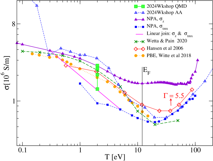
Figure 1: (Color online) The isochoric conductivities $\sigma_{z},\sigma_{tmx}$ calculated via the Ziman formula with NPA inputs, for $l$-aluminum, are compared with representative AA, QMD and other results. Results given in Ref. Stanek24 are labeled “2024 Wkshop”.The five QMD results at 2 eV use several different XC-functionals. Witte et al, 2018 WittePOP18 refers to QMD calculations using the $T=0$ Perdew-Burke-Ernzerhof XC-functional. Wette & Pain 2020 Pain20 ; Hansen et al 2016 Hansen2006 . The value of $E_{F}$ displayed corresponds to $\bar{Z}\sim 3$, but this increases as $T$ increases, as seen in Table 3.

As first noted by Perrot and the present author in 1999 Thermophys99 , these results confirm that $\sigma_{z}$ from pseudopotential-based calculations, and $\sigma_{tmx}$ from T-matrix based calculations, differ significantly. The differences appear when Al³⁺ begins to loose core electrons, with $\bar{Z}$ increasing beyond three. The Al³⁺ ion has a robust filled core with the electronic configuration: $1s^{2}2s^{2}3p^{6}$. An electron moving under an applied field will scatter from it elastically, with no interaction with the core except for a form factor already included in the weak pseudopotential. Interactions between continuum electrons and core electrons are possible but these are not elastic collisions (where the energy change $\omega\neq 0$).

$$U_{ei}(k) = \Delta n_{f}(k)/\chi(k)$$ (23)

$$\chi(k) = \chi^{0}(k)/\left[1+v_{k}(1-G_{k})\chi^{0}(k)\right]$$ (24)

Here $v_{k}=4\pi/k^{2}$, and $\chi^{0}(k)$ is the Lindhard function for non-interacting electrons. The local-field correction $G_{k}$ contains XC-corrections. The use of the pseudopotential corresponds to the use of the Hamiltonian

$$H=H_{0}+\sum_{\vec{k},\vec{k}_{1},\vec{k}_{2}}U_{ei}(k)A^{\dagger}_{\vec{k}_{1}}a^{\dagger}_{(\vec{k}_{2}+\vec{k})}a_{\vec{k}_{2}}A_{(\vec{k}_{1}+\vec{k})}+\mbox{other terms}$$ (25)

Here $A^{\dagger}_{\vec{k}},A_{\vec{k}}$ are creation and annihilation operators for ions, while $a^{\dagger}_{\vec{k}},a_{\vec{k}}$ are for electrons. The matrix elements are written to indicate momentum conservation to be formally exact, but this is irrelevant for massive ions usually treated in the Lorentz plasma model; the momenta of ion-density fluctuations $\rho^{\dagger}_{k}=\sum_{\vec{k}_{1}}A^{\dagger}_{\vec{k}_{1}+\vec{k}}A_{\vec{k}_{1}}$ are not conserved unless ion dynamics is included.

If the ion core is robust, and if $U_{ei}(k)$ is weak, as is the case for Al³⁺, multiple scattering effects, strong-collisions etc., are negligible and the T-matrix results should agree with those from the weak pseudopotential. Numerical limitations in our codes prevent us from extending the T-matrix calculation of the conductivity to low temperatures to verify this explicitly. In fact, our $\sigma_{tmx}$ for Al becomes increasingly inaccurate for $T<3$ eV. In fig. 1 we have joined the $\sigma_{z}$ with $\sigma_{tmx}$ with a straight line to indicate the transition region where the pseudopotential model begins to breakdown, while the T-matrix method becomes appropriate. In this region core states acquire partial occupancies while $\bar{Z}>3$ has a fractional value and an integer part.

The partial occupancies in the core provide a mechanism for some of the conduction electrons to become “hopping electrons” hop1992 , and the value of the conductivity depends on how these electrons are treated in the conductivity model. Partial occupancies of core states make it possible for continuum electrons to interact with core electrons while the overall energy is conserved, as in elastic collisions, while the momentum need not be conserved as the ions are assumed to be infinitely heavy. For instance, an electron in a $k,l$ state of energy $k^{2}/2$ may fall into a partially occupied $3p$ state while an electron in such a $3p$ may be ejected to a $k,l^{\prime}$ state of energy $k^{2}/2$. That is, the T-matrix approach includes additional scattering channels that are not included in the ion with a rigid-core implied by the pseudopotential $U_{ei}(k)$.

The phase shifts that are used to construct the T-matrix are such that:
(i) they satisfy the finite-$T$ Friedel sum rule DWP82 that sets the value of $\bar{Z}$ self-consistently with the ionization balance and thermodynamics;
(ii) they provide a consistent treatment of strong collisions that takes account of the partially ionized states of the core and any continuum resonances.

Given that the numerical results of the pseudopotential model differ very significantly from the strong-collisions model already at, say, $T=2$ eV, one would wonder why the pseudopotential model is successful in accurately predicting the pair-distribution functions of $l$-Al at 1 eV, or 2 eV, etc., in the sense that the $g(r),S(k)$ obtained from the NPA pair-potentials agree very well from QMD calculations. The agreement of NPA pair-distribution functions with those of QMD has been demonstrated in many previous publications (e.g., HarbourDSF18 ; DW-yuk22 ). The reason for this is that the ion-ion pair potential involves a strong repulsive term $\bar{Z}^{2}V_{k}$, which is not there in the electron-ion interaction. The latter is essentially an attractive interaction that encourages close collisions; furthermore, any Pauli blocking that exists in fully occupied core states is removed for partial occupancies.

These same issues affect the accuracy of the Kubo-Greenwood approach in calculating a $\sigma(\omega)$ and extrapolating to $\omega\to 0$ via some rigid-core model, e.g., the Drude model. The sensitivity of $\sigma_{K-G}$ obtained from QMD to the XC-functionals emphasizes this difficulty. In Fig. 1, the QMD K-G $\sigma$ for Al at 2.7g/cm³ takes the highest value of 2.6$\times 10^{6}$ S/m for a calculation using the PBE functional, while the lowest value is nearly half, viz., 1.38$\times 10^{6}$ S/m is for the SCAN functional. It should be noted that as the number $N$ of ions used in a QMD simulation increases, the complex character of possible ionic configurations of “bonding schemes” increases, and the corresponding electron distributions become very complex, demanding more and more complex XC-functionals. In contrast, in the NPA and in AA models there is only one ion and the corresponding electron density is a simple smooth density with the main rapid changes and discontinuity being at the nucleus. Consequently, NPA calculations are insensitive to the XC-functional used.

Furthermore, since QMD implementations do not usually incorporate finite-$T$ XC-functionals, the corrections to the specific heat from XC-effects are not included in such calculations, thus affecting the calculation of $\kappa$.

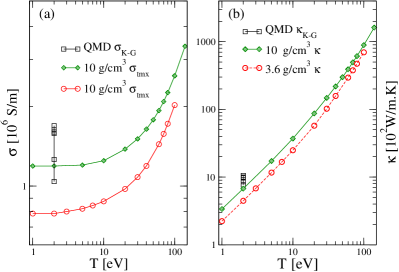
Figure 2: (Color online) (a) The isochoric conductivities $\sigma_{tmx}$ for $l$-carbon at 10 g/cm³ and 3.6g/cm³ from NPA calculations. (b) The corresponding NPA-$\kappa$ obtained via the Lorentz number $L_{n}(t)$. The QMD results for $\sigma$ and $\kappa$ for $l$-C at 10 g/cm³, $T$=2 eV reported in Ref. Stanek24 are also displayed.

IV Tabulated data for Aluminum and Carbon

In this section we provide some representative results for isochoric $\sigma$ and $\kappa$ for $l$-carbon, and $l$-aluminum at 2.70 g/cm³. The $l$-carbon data are at the density 10.0 g/cm³ and at the “diamond-like” density of 3.6 g/cm³. The $\sigma_{tmx}$ is calculated using the NPA, and $\kappa$ is obtained from the numerical fit to the Lorentz number $L_{N}(t)$.

A sample of tabulated results for $l$-carbon at 10 g/cm³ is give in table 1

Table 1: The isobaric conductivity $\sigma_{tmx}$, and $\kappa$ for $l$-C at 10 g/cm³. The thermal conductivity is calculated from $\sigma$ using the finite-$T$ Lorentz number $L_{N}(t)$ defined in the main text. More digits than warranted by physical accuracy are shown for technical reasons (e.g., useful in identifying the version of a code used to generate the results).

Tev	$\sigma_{tmx}$	$\bar{Z}$	$\kappa/10^{2}$
1	1.190	4.000	3.373
2	1.190	4.000	6.743
5	1.191	4.000	16.89
10	1.246	4.000	35.34
20	1.378	4.000	78.40
40	1.640	4.003	193.4
60	1.927	4.042	365.2
80	2.252	4.158	595.4
100	2.608	4.337	879.6
140	3.369	4.733	1613

At low temperatures, the resistivity “saturates” as the $l$-carbon structure factor adjusts to have a maximum at 2$k_{F}$ as $T/E_{F}\to 0$, when electron-ion scattering is maximized as in Friedel-controlled fluids DW-yuk22 . We see essentially the same behaviour in carbon at the “diamond-like” density of 3.6 g/cm³, (see Table 2). The data for $l$-carbon at these two densities are displayed in Fig. 2.

Table 2: The isobaric conductivity $\sigma_{tmx}$, and $\kappa$ for $l$-C at 3.6 g/cm³. The thermal conductivity is calculated from $\sigma$ using the finite-$T$ Lorentz number $L_{N}(t)$ defined in the main text.

Tev	$\sigma_{tmx}$	$\bar{Z}$	$\kappa/10^{2}$
1.0	0.787	4.000	2.233
2.0	0.787	4.000	4.464
3.0	0.801	4.000	6.813
5.0	0.821	4.000	11.64
10.0	0.875	4.000	24.89
20.0	0.975	4.000	57.41
40.0	1.191	4.005	157.6
60.0	1.438	4.073	294.5
80.0	1.719	4.267	472.4
100.0	2.021	4.530	695.5

Table 3: The isobaric conductivity $\sigma_{tmx}$ ($\sigma_{z}$ if in parenthesis), and $\kappa$ for $l$-Al at 2.7 g/cm³. The thermal conductivity is calculated from $\sigma$ using the finite-$T$ Lorentz number $L_{N}(t)$ defined in the main text. More digits than warranted by physical accuracy are shown for technical reasons (e.g., useful in identifying the version of a code used to generate the results).

Tev	$\sigma_{tmx}$	$\bar{Z}$	$\kappa/10^{2}$
0.1	(4.60)	3.000	1.303
0.3	(3.89)	3.000	3.309
5	0.796	3.000	12.83
8	0.678	3.003	15.98
10	0.631	3.016	21.19
20	0.566	3.495	38.62
30	0.615	4.299	63.22
40	0.703	5.085	96.55
60	0.860	6.233	177.5
80	1.046	7.296	288.2
100	1.152	7.720	396.9

References

- (1) N. W. Ashcroft and N. D. Mermin, Solid State Physics, Ch. 13. Saunders College, Philadelphia, USA (1976).
- (2) E. M. Lifshitz and L. P. Pitaevaskii, Physical Kinetics, Pergamon, New York (1981).
- (3) M. W. C. Dharma-wardana and F. Perrot, Phys. Rev. A 26, 2096 (1982).
- (4) F. Perrot and M.W.C. Dharma-wardana, Phys. Rev. E. 52, 5352 (1995).
- (5) V. Recoules and J. P. Crocombette, Phys. Rev. B 72, 104202 (2005).
- (6) F. Perrot and M. W. C. Dharma-wardana, Phys. Rev. B 62, 16536 (2000); Erratum: 67, 79901 (2003); arXive-1602.04734.
- (7) F. Perrot and M. W. C. Dharma-wardana, Phys. Rev. A 30, 2619 (1984).
- (8) Ethan W. BrownJ. L. DuboisJ. L. Dubois, Markus Holzmann, David Ceperley Phys. Rev B 88, 081102(R) (2013).
- (9) V. V. Karasiev, T. Sjostrom, J. W. Dufty, and S. B. Trickey, Phys. Rev. Lett. 112, 076403 (2014).
- (10) Tobias Dornheim, Simon Groth, Michael Bonitz Physics Reports, 744, 1-86 (2018), https://doi.org/10.1016/j.physrep.2018.04.001.
- (11) V. Karasiev, S. B. Trickey and J. W. Dufty. Phys. Rev. B 99, 195134 (2019).
- (12) M. W. C. Dharma-wardana J. Phys. C. 9, 1919 (1976).
- (13) C. F. Richardson and N. W. Ashcroft, Phys. Rev. B 50, 8170 (1994).
- (14) M. W. C. Dharma-wardana, Physica, 92A, 59-86 (1978).
- (15) L. Spitzer and R. Härm, Phys. Rev. 89, 977 (1953).
- (16) H. Reinholz, G. Röpke, S. Rosmej, and R. Redmer, Phys. Rev. E 91, 043105 (2015).
- (17) L. J. Stanek, A. Kononov, S. B. Hansen, et al. Review of the Second Chared-Particle Transport Coefficient Code-Comparison Workshop. Unpublished (2023).
- (18) B. B. L. Witte, P. Sperling, M. French, V. Recoules, S. H. Glenzer, and R. Redmer, Physics of Plasmas 25, 056901 (2018).
- (19) F. Perrot and M. W. C. Dharma-wardana, Int. J. of Thermophys, 20, 1299 (1999).
- (20) M.W.C. Dharma-wardana and F. Perrot, Phys. Rev. A 45, 5883 (1992).
- (21) L Harbour, and G. D. Förster, M. W. C. Dharma-wardana and Laurent J. Lewis, Physical review E 97, 043210 (2018).
- (22) M. W. C. Dharma-wardana, Lucas J. Stanek, and Michael S. Murillo Phys. Rev. E 106, 065208 (2022).
- (23) N. Wetta and J.-C. Pain, Phys. Rev. E 102, 053209 (2020).
- (24) S. B. Hansen, W. A. Isaacs, P. A. Sterne, B. G. Wilson, V. Sonnad, D. A. Young Proceedings of the NEDPC2005; Technical Report: UCRL-PROC-218150 Lawrence Livermore (US) National laboratory, Livermore, USA (2006).