Enhanced twist-and-turn dynamics of spin squeezing in internal bosonic Josephson junctions

Abstract

The twist-and-turn dynamics of spin squeezing results from the interplay of the (nonlinear) one-axis-twisting- and the (linear) transverse-field turning term in the underlying Hamiltonian, both with constant (time-independent) respective coupling strenghts. Using the methods of shortcuts to adiabaticity (STA) and their recently proposed enhanced version (eSTA), we demonstrate here that dynamics of this type can be utilized for a fast and robust preparation of spin-squeezed states in internal bosonic Josephson junctions – condensates of cold bosonic atoms in two different internal (hyperfine) states (single-boson modes). Assuming that the initial state of this system is the coherent spin state with all the bosons in the equal superposition of the two single-boson modes and that the nonlinear-coupling strength in this system remains constant, we set out to determine the time-dependence of the linear-coupling strength using the STA and eSTA approaches. We then quantitatively characterize the modified twist-and-turn dynamics in this system by evaluating the coherent spin-squeezing- and number-squeezing parameters, as well as the fidelity of the target spin-squeezed states. In this manner, we show that the eSTA approach allows for a particularly robust experimental realization of strongly spin-squeezed states in this system, consistently outperforming its adiabatic and STA-based counterparts, even for systems with several hundred particles.

I Introduction

Recent years have witnessed tantalizing progress in the realm of quantum-state engineering Sto (a); Pen ; Sto (b); Zhe ; Haa (a); Zha (a, b); Erh ; Haa (b); Qia ; Fen ; Nau ; Sto (c); StoSal ; StefPaspa ; Wu+ ; Sto (d). Being highly interwoven with the constant improvement of methods for manipulation and control of quantum systems, this steady progress remains of pivotal importance for further development of quantum-enhanced technologies in various physical platforms Dow . In particular, prompted by the anticipated quantum-technology applications of highly entangled multiqubit states a large variety of schemes for fast (compared to the relevant coherence time of the underlying physical system) and robust (against various system-specific sources of decoherence and noise) generation of such states have been proposed in recent years, especially for $W$ Sto (a); Pen ; Sto (b); Zhe ; Haa (a); Zha (a, b), Greenberger-Horne-Zeilinger (GHZ) Erh ; Haa (b); Qia ; Fen ; Nau ; Sto (c), and Dicke Wu+ ; Sto (d) states. Another important example of highly-entangled quantum many-body states of interest for quantum-enhanced metrology is furnished by spin-squeezed states Kit .

Proposed in the seminal work of Kitagawa and Ueda Kit , the concept of spin squeezing – i.e., that of redistributing the spin fluctuations between two orthogonal directions – was demonstrated to allow an enhancement in the precision of atom interferometers Wine ; Win . Much like their photonic counterparts in optical interferometry Cav , spin-squeezed states provide phase sensitivities beyond the standard quantum limit (SQL) for phase uncertainty $\Delta\Theta_{\textrm{SQL}}=1/\sqrt{N}$, the latter being characteristic of probes involving a finite number $N$ of uncorrelated (or classically correlated) particles Gio . Owing to the fact that they allow one to overcome this classical bound, spin-squeezed states established themselves as a valuable resource for quantum metrology Pez . Subsequently, the important link between spin squeezing and entanglement – the ingredient that spin-squeezed states share with other types of states defying the SQL (for instance, GHZ states Lee ) – was also established Sor (a, b).

In their original work, Kitagawa and Ueda investigated the preparation of spin-squeezed states based on one-axis twisting (OAT) and two-axis-countertwisting (2ACT) Hamiltonians, where “twisting” refers to terms that are quadratic in the collective spin operators Kit . While both of these Hamiltonians permit the generation of spin-squeezed states, they show qualitatively different behavior. The OAT Hamiltonian does not saturate the fundamental quantum-metrological bound of sensitivity and leads to the maximal squeezing at a time that scales as $J^{1/\mu}$, where $J$ is the size of the collective spin and $\mu>0$. In contrast to its OAT counterpart, the 2ACT Hamiltonian does saturate the fundamental quantum-mechanical limit on sensitivity and permits the generation of maximal spin squeezing in a time that is logarithmic in the collective-spin size. Subsequently, a model that in addition to the (nonlinear) OAT term involves a linear term describing a transverse field was also investigated by Micheli et al. Mich (b). For this type of spin-squeezing Hamiltonian, which gives rise to what became known as twist-and-turn (TNT) dynamics Haho ; Huho , they demonstrated that it allows the preparation of highly entangled metrologically-relevant states (cat-like states) at times that are – similar to the 2ACT case – logarithmic in the size of the collective spin Mich (b). Finally, in a study complementary to that of Ref. Mich (b), it was demonstrated that this type of dynamics is optimal as far as the generation of spin squeezing is concerned Sor (c), at least in the absence of decoherence and losses.

The most natural physical setting in which to demonstrate the TNT dynamics of spin squeezing and harness the latter for generating strongly spin-squeezed states is provided by Bose-Einstein condensates (BECs) of cold neutral atoms. Indeed, the generation of spin-squeezed states was demonstrated more than a decade ago in proof-of-principle experiments with interacting cold ⁸⁷Rb atoms in bosonic Josephson junctions (BJJs)  Est ; Gro (b); Rie ; Zib ; these systems, where bosons within a condensate can be restricted to occupy only two single-atom states (modes), come in two varieties: internal BJJs [where the two relevant modes correspond to two different internal (hyperfine) atomic states, with a linear, Rabi-type coupling between them] and external ones (in which the two modes correspond to bosons trapped in two spatially separated wells of an external double-well potential) Gat . The TNT-type dynamics was experimentally investigated in an internal BJJ, assuming a constant linear-coupling strength and an abrupt change (i.e. a quench) of a nonlinear-coupling strength from zero to a finite value Muessel+:15 . Finally, an alternative approach for generating spin squeezing in internal BJJs has quite recently been theoretically proposed Odelli+:23 , which makes use of the methods of shortcuts to adiabaticity (STA) Chen2010STA ; chen2010b ; ibanez2012 ; torrontegui2013a ; STA_RMP:19 and their recently proposed enhanced version (eSTA) Whitty+:20 ; Whitty+:22 ; Whitty2022b .

STA are a family of analytical control techniques that mimic adiabatic evolutions, but are typically much faster than their adiabatic counterparts Chen2010STA ; chen2010b ; ibanez2012 ; torrontegui2013a ; STA_RMP:19 . Generally speaking, analytical control approaches are highly desirable because they are usually rather simple, in addition to providing greater physical insight and allowing for superior stability under various experimental imperfections ruschhaupt2012a ; lu2020 . STA have heretofore been utilized in many different contexts, e.g. li2022 ; kiely2016 ; kiely2018 ; torrontegui2011 , including the proposals for the generation of spin-squeezed states in BJJs Jul (a, b); besides, their use was also proposed for engineering other types of entangled states (such as, e.g., NOON states Hat ; Ste ). They proved to yield results comparable to those originating from optimal-control schemes Lap ; Sor (c).

One typical limitation of STA methods is that they often require non-trivial physical implementation (e.g. counterdiabatic driving STA_RMP:19 ); likewise, some STA techniques can only be straightforwardly applied to small or highly symmetric systems (e.g. methods based on Lewis-Riesenfeld invariants) STA_RMP:19 . This served as the primary motivation behind the development of Enhanced Shortcuts to Adiabaticity (eSTA) Whitty+:20 ; Whitty+:22 ; Whitty2022b , an approach that allows one to perturbatively improve STA solutions in an analytical fashion and, even more importantly, design efficient control protocols for systems in which STA are not directly applicable. The eSTA method was shown to outperform its STA counterparts in nontrivial quantum-control problems related to coherent atom transport in optical lattices Whitty+:20 ; Hau (a, b) and anharmonic trap expansion Whitty2022b . Besides, it was demonstrated that eSTA-based control schemes are more robust against various types of imperfections than those based on STA methods Whitty+:22 .

In this paper, we revisit the problem of efficiently preparing spin-squeezed states in internal BJJs by modifying the underlying TNT-type dynamics of spin squeezing in this system. In particular, we assume that the initial state of the system under consideration is the coherent spin state (CSS) with all bosons occupying the same single-particle state – namely, the equal superposition of the two single-boson modes. We also assume that the nonlinear-coupling strength in this system remains constant (i.e. time-independent) and subsequently determine the time-dependence of the linear-coupling strength that allows the preparation of spin-squeezed states using the STA and eSTA methods; we also compare the performance of the latter methods with their adiabatic counterpart - a simple linear sweep of the linear-coupling strength from a large initial- to a small final value. We then quantify the state-preparation process for the desired spin-squeezed states in this system by computing the values of the coherent spin-squeezing- and number-squeezing parameters, as well as the target-state fidelity. In this way, we show that our proposed eSTA-based control scheme allows for a particularly robust experimental realization of strongly spin-squeezed states in internal BJJs. Importantly, we demonstrate that this approach consistently outperforms its STA-based and adiabatic counterparts, even for particle numbers that are in the range of several hundreds.

The remainder of this paper is organized in the following manner. In Sec. II, we set the stage for further discussion by briefly reviewing the essential physics of internal BJJs and introducing their underlying Lipkin-Meshkov-Glick-type Hamiltonian; we also introduce the relevant figures of merit for characterizing spin squeezing. Section III is dedicated to the details of the eSTA formalism as applied to the system at hand. In Sec. IV we present the obtained results for the target-state fidelities and spin-squeezing parameters computed within the proposed eSTA-based scheme; we also compare those results with those corresponding to the conventional STA approach. In this section, we also demonstrate the superior robustness of our proposed, eSTA state-preparation scheme to the STA-based one. The paper is summarized, with some concluding remarks and outlook, in Sec. V.

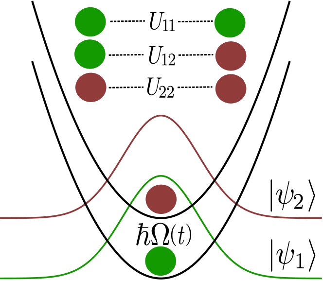
Figure 1: Pictorial illustration of an internal BJJ, i.e. a condensate of bosons in two different hyperfine states (modes) $|\psi_{1}\rangle$ and $|\psi_{2}\rangle$. An external electromagnetic field coherently transfers atoms between these two modes (Rabi rotations); the corresponding linear (Rabi-type) coupling strength $\hbar\Omega$ is assumed to depend on time. The intraspecies interaction strengths $U_{11}$ and $U_{22}$, as well as their interspecies counterpart $U_{12}$, are assumed to be time-independent. The value of $U_{12}$ can be suppressed by means of an external magnetic field in the presence of a Feshbach resonance, leading to an increase in the nonlinear coupling strength $\chi=(U_{11}+U_{22}-2U_{12})/\hbar$.

II System and engineering of spin-squeezed states

II.1 Internal BJJs and their underlying many-body Hamiltonian

An internal BJJ is created with a trapped BEC that consists of cold atoms in two different internal (hyperfine) states Ste (for a pictorial illustration, see Fig. 1 below). A typical example of such a system is a condensate of ⁸⁷Rb atoms, where the role of the two relevant internal states can, for example, be played by the $|F=1,m_{\textrm{F}}=1\rangle$ and $|F=2,m_{\textrm{F}}=-1\rangle$ hyperfine sublevels of the electronic ground state of rubidium. Assuming that the external atomic motion in such a system is not affected by internal dynamics, it is pertinent to use a single-mode approximation for atoms in each of the two hyperfine states; these two single-boson modes will in the following be denoted by $|\psi_{1}\rangle$ and $|\psi_{2}\rangle$. An internal BJJ is typically prepared by trapping the atoms in the two internal states within the wells of a deep one-dimensional optical lattice; the depth of such a lattice ought to be sufficiently large that coherent tunnelling of atoms between different wells is suppressed Gro (b).

The linear, Rabi-type, coupling of atoms in the two relevant internal states of an internal BJJ is enabled by an electromagnetic field that coherently transfers atoms between those states by means of Rabi rotations Hal . At the same time, atoms interact through $s$-wave two-body interactions (nonlinear coupling), both atoms in the same internal state (intraspecies interaction) and those in different states (interspecies interaction). As a result, an internal BJJ is described by a two-state Bose-Hubbard model. Using the Schwinger-boson formalism (see, e.g., Pez ), the corresponding Hamiltonian can be written in the form

$$H_{\textrm{IBJJ}}(t)=\hbar\chi J_{z}^{2}-\hbar\Omega(t)J_{x}\>,$$ (1)

which represents a special case of the Lipkin-Meshkov-Glick family of Hamiltonians Lip . Here $\hbar\Omega$ is the strength of Rabi-type coupling; in the problem at hand, this linear-coupling strength is assumed to depend on time, i.e., $\Omega=\Omega(t)$. The nonlinear-coupling strength $\chi$ is assumed to be constant and positive (corresponding to repulsive two-body interactions between atoms) in the following. $\mathbf{J}\equiv\{J_{x},J_{y},J_{z}\}$ are pseudoangular-momentum operators describing the collective spin of bosons, which is defined as $\mathbf{J}=\sum_{k}\boldsymbol{\sigma}^{(k)}$, with $\boldsymbol{\sigma}^{(k)}\equiv\{\sigma^{(k)}_{x},\sigma^{(k)}_{y},\sigma^{(k)}_{z}\}$ being the Pauli operators representing the pseudospin degree of freedom of the $k$-th atom ($k=1,2,\ldots,N$). These pseudoangular-momentum operators, which satisfy the standard commutation relation $[J_{k},J_{l}]=i\hbar\sum_{m}\epsilon_{klm}J_{m}$ of the $su(2)$ algebra (where $k,l,m=x,y,z$ and $\epsilon_{klm}$ is the Levi-Civita symbol), are given by

$$J_{x} = \frac{1}{2}\>(J_{+}+J_{-})\>,$$

$$J_{y} = \frac{1}{2i}\>(J_{+}+J_{-})\>,$$ (2)

$$J_{z} = \frac{1}{2}\>(n_{1}-n_{2})\>.$$ (3)

In terms of the creation and annihilation operators $a^{\dagger}_{i}$ and $a_{i}$ ($i=1,2$) corresponding to the two relevant single-boson modes, the operators $J_{\pm}$ are expressed as $J_{+}=a^{\dagger}_{2}a_{1}$, $J_{-}=a^{\dagger}_{1}a_{2}$, and $n_{1,2}$ as $n_{1}=a^{\dagger}_{1}a_{1}$, $n_{2}=a^{\dagger}_{2}a_{2}$.

It is important to point out that in a system described by the Hamiltonian with $J_{z}^{2}$ and $J_{x}$ terms [cf. Eq. (1)], the mean collective spin points in the direction of $J_{x}$ and the direction of minimal variance is that of $J_{z}$ [cf. Eq. (2)]; the length of the collective spin is $J\equiv N/2$.

The linear-coupling strength in the Hamiltonian $H_{\textrm{IBJJ}}(t)$ [cf. Eq. (1)] is given by

$$\Omega=\Omega_{R}\int d^{3}\mathbf{r}\>\psi^{*}_{1}(\mathbf{r})\psi_{2}(\mathbf{r})\>,$$ (4)

where $\Omega_{R}$ stands for the Rabi frequency and $\psi_{i}(\mathbf{r})\equiv\langle\mathbf{r}|\psi_{i}\rangle$ ($i=1,2$) are the two internal states in the coordinate representation (i.e. the mode functions of those states). The time dependence of the linear-coupling strength $\Omega=\Omega(t)$ can be manipulated with a high degree of control; for instance, this can be accomplished experimentally by controlling the magnitude of the electromagnetic field used. Importantly, the existing experimental capabilities allow for making rapid changes in both the amplitude and the phase of $\Omega(t)$ Muessel+:15 .

The nonlinear-coupling strength $\chi$ is given by

$$\hbar\chi=U_{11}+U_{22}-2U_{12}\>,$$ (5)

where $U_{ij}$ ($i,j=1,2$) are the (two-body) $s$-wave intraspecies ($i=j$) and interspecies ($i\neq j$) interaction strengths. The latter can be expressed as

$$U_{ij}=\frac{2\pi\hbar^{2}a^{(i,j)}_{s}}{M}\int d^{3}\mathbf{r}|\psi_{i}(\mathbf{r})|^{2}|\psi_{j}(\mathbf{r})|^{2}\>,$$ (6)

where $a^{(i,j)}_{s}$ ($i,j=1,2$) are the corresponding $s$-wave scattering lengths and $M$ is the mass of a single atom. It is important to stress that the interspecies $s$-wave scattering length $a^{(1,2)}_{s}$ for ⁸⁷Rb atoms can be tuned using an external magnetic field owing to the presence of Feshbach resonance Zib ; this mechanism can be utilize to reduce the interspecies $s$-wave scattering length, given that for ⁸⁷Rb atoms there is a nearly perfect compensation of intraspecies and interspecies interactions. Another approach for tuning the nonlinear-coupling strength $U$ relies on controlling the wave-function overlap between the two internal states in a state-dependent microwave potential Rie . The main advantage of the latter approach is that it also works in magnetic traps and in the absence of a convenient Feshbach resonance for the relevant pair of internal atomic states.

The Hamiltonian of the system under consideration [cf. Eq. (1)] is given by the sum of the nonlinear OAT term $\hbar\chi J_{z}^{2}$ and the Rabi-coupling (turning) term $-\hbar\Omega(t)J_{x}$; the latter describes a time-dependent rotation around the $J_{x}$ axis, with the rotation rate $\Omega(t)$. Therefore, this Hamiltonian describes modified – due to the presence of time-dependent $\Omega(t)$ – TNT-type dynamics of spin squeezing in internal BJJs. The dimensionless parameter $\Lambda\equiv N\chi/\Omega$ is conventionally used to quantify the relative importance of the nonlinear- and Rabi couplings in an internal BJJ Gro (a). Because in the problem at hand we assumed that Rabi coupling is time-dependent [i.e. $\Omega=\Omega(t)$], the parameter $\Lambda$ will also have a nontrivial time-dependence in what follows.

Generally speaking, we can distinguish three different regimes for a system described by the Hamiltonian in Eq. (1). The Rabi regime corresponds to the noninteracting limit ($\Lambda\ll 1$) of such a system, where its ground state is a CSS with maximal mean collective-spin length $\langle J_{x}\rangle=N/2$ and equal spin fluctuations in the orthogonal directions (i.e. variances $\Delta J_{y}^{2}=\Delta J_{z}^{2}=N/4$). The latter is a special case of more general CSSs $|\theta,\phi\rangle\equiv e^{-i\phi J_{z}}e^{-i\theta J_{y}}|J,J\rangle$, where $\theta$ and $\phi$ are the spherical polar angles ($0\leq\theta<\pi$, $0\leq\phi<2\pi$) and $|J,J\rangle$ is the joint eigenstate of $J^{2}$ and $J_{z}$ with the highest possible value (equal to $J=N/2$) of $J_{z}$. This state corresponds to all $N$ atoms being in the same single-particle state – namely, an equal linear combination of the two modes $|\psi_{1}\rangle$ and $|\psi_{2}\rangle$ – and is characterized by the complete absence of quantum correlations between particles; it is given by

$$|\theta=\pi/2,\phi=0\rangle=\frac{1}{\sqrt{2^{N}N!}}\>(a^{\dagger}_{1}+a^{\dagger}_{2})^{N}|\textrm{vac}\rangle\>,$$ (7)

where $|\textrm{vac}\rangle$ is the vacuum state.

In the presence of increased interactions ($1<\Lambda<N$), fluctuations in the relative atom number in the two modes – which translates to fluctuations in $J_{z}$ – become energetically unfavorable. This is the Josephson regime, in which the ground state is a coherent spin-squeezed state, in which the spin fluctuations in the $J_{z}$ direction are reduced at the expense of increased fluctuations in the $J_{y}$ direction and reduced mean collective-spin length. Finally, in the strongly-interacting case (Fock regime), i.e. for $\Lambda\gg N$, the ground state of the system is a strongly spin-squeezed state with vanishing mean collective-spin length.

It is pertinent to note that the Hamiltonian of the system under consideration [cf. Eq. (1)] is invariant under the exchange of the single-boson modes $|\psi_{1}\rangle$ and $|\psi_{2}\rangle$. Namely, under the transformation $a_{1}\leftrightarrows a_{2}$, we have that $J_{x}\rightarrow J_{x}$ and $J_{z}\rightarrow-J_{z}$, thus the Hamiltonian in Eq. (1) remains unchanged. Therefore, the system under consideration possesses a parity symmetry, which in turn guarantees the symmetry-protected adiabatic evolution Zhu . Indeed, in the $\chi>0$ case discussed here one possible route towards generating spin-squeezed states is the adiabatic evolution. By initially setting $\Omega(t=0)$ to be sufficiently large and adiabatically sweeping $\Omega(t)/\chi$ to zero, the state obtained from the original CSS will remain an instant ground state of the Hamiltonian of the system and spin-squeezed states (with the same parity) are obtained when $\Omega(t)/\chi$ is close to zero. The simplest way to achieve this is to perform a linear sweep, i.e. $\Omega(t)=\Omega(0)+v_{\Omega}t$. Provided that the constant sweeping rate $v_{\Omega}<0$ is sufficiently small, such an adiabatic evolution of the ground state of the system can be achieved with high fidelity. However, this adiabatic approach for the preparation of spin-squeezed states requires long preparation times, hence motivating one to employ a different, more time-efficient, strategy.

In the following, we set out to determine the time-dependence $\Omega(t)$ of the linear-coupling strength [or, equivalently, that of the parameter $\Lambda(t)$] that allows the preparation of a spin-squeezed state at the time $t=t_{f}$, starting from the CSS in Eq. (7) as the initial ($t=0$) state. This state-control problem will in what follows be addressed using the STA and eSTA approaches (see Sec. III below). Importantly, both the initial- and final states in our envisioned state-preparation scheme are ground states of the total system Hamiltonian at the respective times $t=0$ and $t=t_{f}$. While this is – in general – not a requirement for the application of the STA- and eSTA methods STA_RMP:19 , this circumstance does away with the need to freeze the system dynamics once the sought-after spin-squeezed state is prepared, thus making our state-preparation scheme more robust.

II.2 Figures of merit for spin squeezing

Because in the present work we will be concerned with the preparation of spin-squeezed states, it is pertinent to introduce the figures of merit that can be used to quantify spin squeezing in the system at hand. Two important figures of merit that can be used for this purpose are the number-squeezing- and coherent spin-squeezing parameters.

The number-squeezing parameter, also known as the Kitagawa-Ueda spin-squeezing parameter, is defined as Wine

$$\xi^{2}_{N}(t)=\frac{\Delta J^{2}_{z}}{(\Delta J_{z}^{2})_{\text{bin}}}=\frac{\Delta J^{2}_{z}}{N/4}\>,$$ (8)

with $\Delta J^{2}_{z}\equiv\langle J^{2}_{z}\rangle-\langle J_{z}\rangle^{2}$ being the variance of the operator $J_{z}$; the time argument on the left-hand-side of Eq. (8) reflects the fact that in the time-dependent state-preparation problem under consideration the parameter $\xi^{2}_{N}$ also depends on time. In Eq. (8), $J/2=N/4$ (the shot-noise limit) corresponds to the CSS with $\langle J_{z}\rangle=0$. Accordingly, a many-body state is considered number-squeezed ($\xi_{N}<1$) provided that the corresponding variance of one spin component is smaller than the shot-noise limit.

The coherent spin-squeezing parameter, which is often referred to as the Wineland parameter and in the problem at hand is time dependent, is given by Sor (a)

$$\xi^{2}_{S}(t)=\frac{N\Delta J^{2}_{z}}{\langle J_{x}\rangle^{2}}=\frac{\xi^{2}_{N}(t)}{\alpha^{2}(t)}\>,$$ (9)

where $\alpha(t)\equiv\langle\Psi(t)|2J_{x}/N|\Psi(t)\rangle$ quantifies the phase coherence of the many-body state $|\Psi(t)\rangle$. The parameter $\xi_{S}$ serves to characterize the interplay between an improvement in number squeezing and loss of coherence; it can be used to quantify precision gain in interferometry, given that for spin-squeezed states the interferometric precision is increased to $\Delta\Theta=\xi_{S}/\sqrt{N}$ Gro (a). Furthermore, whenever a many-body state satisfies the inequality $\xi^{2}_{S}<1$ the state in question is entangled Sor (a).

III Improved STA scheme and application of eSTA formalism

In this section, we will present three different approaches to obtain the control function $\Omega(\tau)$ with the goal to drive the system from the initial ground state at $\tau=0$ to the target ground state at $\tau=\tau_{f}$.

The basis of all three schemes is the well-known mapping of the system described by Eq. 1 to the continuum; this mapping will be reviewed first in the following (see Sec. III.1 below).

We will then review the results of yuste2013 and the corresponding STA control scheme $\Omega_{1}$. In the next subsection, we will introduce an improved STA control scheme $\Omega_{2}$. We will then apply the eSTA formalism, proposed and developed by Whitty et al. in Ref. Whitty+:20 , to this improved STA scheme to get an eSTA control scheme $\Omega_{e}$.

III.1 Mapping to the continuum

It is well-known that the two-site (or two-state) Bose-Hubbard model of a BJJ can be mapped to a Schrödinger equation in the continuum with approximately a harmonic potential Mah ; Shc . We will briefly review the main details of this mapping, which will be used frequently in the remainder of this paper.

With $\{\ket{m}\}$ ($m=-N/2,...,N/2$) being the eigenvalues of the operator $J_{z}$, the general state $\ket{\Psi}$ of a BJJ can be written as

$$\ket{\Psi}=\sum_{m=-N/2}^{N/2}c_{m}\ket{m}\>.$$ (10)

The coefficients $c_{m}$ in this expansion ought to satisfy the coupled equations

$$i\hbar\frac{d}{dt}c_{m}(t)$$

$$= -\frac{\hbar\Omega(t)}{2}\left[\beta_{m}c_{m+1}(t)+\beta_{m-1}c_{m-1}(t)\right]+\hbar\chi m^{2}c_{m}(t)\>,$$

where $\beta_{m}=\sqrt{\left(\frac{N}{2}+m+1\right)\left(\frac{N}{2}-m\right)}$. We define now $h=\frac{1}{N/2}$ and $z_{m}=\frac{m}{N/2}$ (the relative population difference between the two relevant hyperfine states). We also switch to the continuum version for the relative population difference ($z_{m}\rightarrow z$), introducing at the same time a dimensionless time $\tau$, such that $t=\tau/\chi$. In this manner, we can recast Eq. (LABEL:eq:numerical) as

$$ih\frac{\partial}{\partial\tau}\psi(\tau,z)$$ (12)

$$= -\frac{\Omega(t)}{\chi}\left[b_{h}(z-h)\psi(\tau,z-h)+b_{h}(z)\psi(\tau,z+h)\right]$$

$$+\frac{N}{2}z^{2}\psi(\tau,z)$$

$$= H_{S}\psi(\tau,z)$$

with

$$b_{h}(z)=\frac{1}{2}\sqrt{\left(1+z+h\right)\left(1-z\right)}\>,$$ (13)

and

$$H_{S}=-\frac{\Omega(t)}{\chi}\left[e^{-ih\partial_{z}}b_{h}(z)+b_{h}(z)e^{ih\partial z}\right]+\frac{N}{2}z^{2}.$$ (14)

We set at this point $b_{h}(z)=0$ for all $z\leq-1-h$ and $z\geq 1$, as well as $\psi(t,z)=0$ for $z\leq-1-h$ and $z\geq 1+h$. It is worthwhile noting that if this equation is satisfied for $z\in[-1-h,1+h]$ (note that it is trivially satisfied outside of this interval) then it is evidently also satisfied for all $z_{m}$ ($m=-N/2,...N/2$) in the previously employed discrete description.

It is interesting to note that if one rewrites the above equation with a different dimensionless time $\bar{\tau}=N\tau$, then the above equation using $\bar{\tau}$ would only depend on the dimensionless quantity $1/\Lambda(t)=\frac{\Omega(t)}{N\chi}$. We will come back to this fact at a later point in the paper.

We now proceed to derive an approximated version of Eq. (12). For small $h$ and by assuming that $z$ is small (i.e. the population difference between the two states is small compared to the total particle number $N$) and neglecting a constant energy shift, we obtain a Schrödinger equation with an approximated Hamiltonian of a harmonic oscillator

$$H_{1}=-h^{2}\frac{\Omega(t)}{2\chi}\frac{\partial^{2}}{\partial z^{2}}+\left[\frac{N}{2}+\frac{\Omega(t)}{2\chi}\right]z^{2}\>.$$ (15)

We can make an additional approximation by assuming that $\frac{N}{2}\gg\frac{\Omega(t)}{2\chi}$, which leads to

$$H_{0}=-h^{2}\frac{\Omega(t)}{2\chi}\frac{\partial^{2}}{\partial z^{2}}+\frac{N}{2}z^{2}\>.$$ (16)

Note that this last Hamiltonian has been the point of departure for deriving the STA scheme in Ref. yuste2013 .

III.2 STA scheme for harmonic approximation $H_{0}$

The STA formalism for the case of internal BJJs is outlined in Ref. yuste2013 . By employing Lewis-Riesenfeld invariants, we can design a solution of the time-dependent Schrödinger equation for the harmonic oscillator Hamiltonian $H_{0}$. By making use of Fourier transform and Lewis-Riesenfeld invariants (for details, see Ref. yuste2013 ), we find that the wave function

$$\chi_{n}(\tau,z) = \frac{\sqrt{b(\tau)}}{\pi^{1/4}\sqrt{2^{n}n!}}\frac{i^{n}\sqrt{k_{0}}}{\sqrt{1-i\beta}}\left(\frac{1+i\beta}{1-i\beta}\right)^{n/2}$$ (17)

$$\times\exp\left(i\varphi(\tau)-\frac{z^{2}b(\tau)^{2}}{2}\frac{k_{0}^{2}}{1-i\beta}\right)$$

$$\times H_{n}\left[\frac{zb(\tau)k_{0}}{\sqrt{1+\beta^{2}}}\right]\>,$$

satisfies the time-dependent Schrödinger equation for the harmonic oscillator Hamiltonian $H_{0}$. Here, we have $k_{0}=\sqrt[4]{\Lambda_{0}}\sqrt{\frac{N}{2}}$ and $\beta=\frac{1}{2\sqrt{\Lambda_{0}}}b(\tau)b^{\prime}(\tau)$. The auxiliary function $b(\tau)$ must be a solution of the Ermakov equation

$$b^{\prime\prime}(\tau)-\frac{N^{2}}{\Lambda_{0}b(\tau)^{3}}+b(\tau)\frac{\Omega(\tau)}{\Omega_{0}}=0\>.$$

We have here also $\varphi(t)=-\int_{0}^{t}ds\,(1+2n)\frac{\sqrt{\Lambda_{0}}}{b(t)^{2}}$. We now employ inverse engineering to first fix a function $b(\tau)$ that satisfies the boundary conditions $b(0)=1$, $b(\tau_{f})=\sqrt[4]{\Omega_{0}/\Omega_{f}}$, $b^{\prime}(0)=b^{\prime}(\tau_{f})=b^{\prime\prime}(0)=b^{\prime\prime}(\tau_{f})=0$. We choose here a polynomial of degree $6$ that satisfies these conditions. By inverting the above equation, we obtain an explicit expression for the sought-after physical control function $\Omega(\tau)$:

$$\Omega(\tau)=\Omega_{0}\left[\frac{1}{b(\tau)^{4}}-\frac{\Lambda_{0}}{N^{2}}\frac{1}{b(\tau)}\frac{\partial^{2}b}{\partial\tau^{2}}\right]\>,$$ (18)

where $\Lambda_{0}\equiv\chi N/\Omega_{0}$. We will call this the first STA scheme in the remainder of this paper and we denote the corresponding control function with $\Omega_{1}$.

III.3 Improved STA scheme for harmonic approximation $H_{0}$

We now proceed to introduce an improved STA scheme. The idea is that while the above approximation is still used for the time evolution, we consider the exact initial and final stated without this approximation for designing the boundary condition of the auxiliary function. In detail, we calculate the exact ground state of the Hamiltonian (15) at initial and final time. For the ground state at initial time $\tau=0$, we get the function of the form of (17) with

$$b(\tau)=\sqrt[4]{1+1/\Lambda_{0}}\>,\quad b^{\prime}(0)=0\>.$$ (19)

For the ground state at final time $\tau=\tau_{f}$, we get the function of the form of (17) with

$$b(\tau_{f})=\sqrt[4]{\frac{\Omega_{0}}{\Omega_{f}}\left(1+\frac{\Omega_{f}}{\Omega_{0}\Lambda_{0}}\right)}\>,\quad b^{\prime}(\tau_{f})=0\>.$$ (20)

We choose now a polynomial satisfying the boundary conditions (19) and (20). In addition, we demand that (18) is also satisfied at the initial- and final times with these new boundary conditions. This leads to two additional boundary conditions

$$b^{\prime\prime}(0) = -\frac{4}{\left(1+1/\Lambda_{0}\right)^{3/4}}\>,$$

$$b^{\prime\prime}(\tau_{f}) = -\frac{4\Omega_{f}/\Omega_{0}}{\left(\Omega_{0}/\Omega_{f}+1/\Lambda_{0}\right)^{3/4}}\>.$$ (21)

We choose here again a polynomial of degree $6$ that satisfies the fix conditions (19),(20) and (21). We will then use (18) with this polynomial to calculate the control function. We will call this the improved STA scheme in the following and will denote the corresponding control function with $\Omega_{2}$.

III.4 eSTA-corrected control function

We will now derive an eSTA correction to the improved STA scheme from the last subsection. The principal idea behind the eSTA formalism is to modify the STA control function by taking into account that the approximated Hamiltonian $H_{0}$ is different from the exact system Hamiltonian $H_{S}$ [cf. Eq. (16)]. Let $\Delta H=H_{S}-H_{0}$ be the difference between these two Hamiltonians and $\boldsymbol{\lambda}=(\lambda_{1},\lambda_{2})$. We consider now the modified control function $\Omega_{e}(\tau)=\Omega_{2}(\tau)+P_{\boldsymbol{\lambda}}(\tau)$. Here, $P_{\boldsymbol{\lambda}}(\tau)$ is a polynomial of degree $4$ that fulfills the following conditions:

$$P_{\boldsymbol{\lambda}}(0)=P_{\boldsymbol{\lambda}}(\tau_{f})=0,$$

$$P_{\boldsymbol{\lambda}}(\tau_{f}/3)=\lambda_{1},P_{\boldsymbol{\lambda}}(2\tau_{f}/3)=\lambda_{2}\>.$$ (22)

These corrections $\boldsymbol{\lambda}$ are calculated by using the formalism of enhanced STA Whitty+:20 ; Whitty2022b .

To begin with, we define the auxiliary functions $G_{n}$, $K_{n}$, and $\mathrm{H}$ that will be used to evaluate $\boldsymbol{\lambda}$. In terms of the STA wave functions $\chi_{n}$ of the approximated Hamiltonian [cf. Eq. (17)] the scalar auxiliary function $G_{n}$ is given by

$$G_{n}=\int_{0}^{t_{f}}dt\innerproduct{\chi_{n}}{\Delta H|\chi_{0}}\>.$$ (23)

The correspionding expression for the vector auxiliary function $\boldsymbol{K}_{n}$ reads

$$\boldsymbol{K}_{n}=\int_{0}^{t_{f}}dt\innerproduct{\chi_{m}}{\boldsymbol{\nabla}H_{S}|\chi_{0}}\>,$$ (24)

with $\boldsymbol{\nabla}H$ being the gradient of the Hamiltonian $H$ with respect to the control parameter $\boldsymbol{\lambda}$. Finally, the matrix elements of $\mathrm{H}$ are given by

$$\mathrm{H}_{l,k}=\sum_{n=1}^{\mathcal{N}}\left[G_{n}(W_{n})_{l,k}+\left(\boldsymbol{K}^{*}_{n}\right)_{k}\left(\boldsymbol{K}_{n}\right)_{l}\right]\>,$$ (25)

where $(W_{n})_{l,k}=\innerproduct{\chi_{n}}{\partial_{\lambda_{l}}\partial_{\lambda_{k}}H_{S}|\chi_{0}}$ stands for a matrix of second derivatives with respect to the control parameter; here $\mathcal{N}$ is the number of STA wave functions that are taken into account.

Having defined the relevant auxiliary functions, we now proceed to compute the correction parameters $\boldsymbol{\lambda}$ using $G_{n}$ and $\boldsymbol{K}_{n}$, assuming that a unit fidelity can be achieved for the exact Hamiltonian Whitty+:20 . The same correction parameters can be obtained in an alternate fashion – namely, by employing the above expressions for $G_{n}$, $K_{n}$, and $\mathrm{H}_{l,k}$ Whitty2022b . By making use of the latter procedure, the correction parameters $\boldsymbol{\lambda}$ are given by

$$\boldsymbol{\lambda}=-\frac{\boldsymbol{v}\norm{\boldsymbol{v}}^{2}}{\boldsymbol{v}^{T}\mathrm{H}\boldsymbol{v}}\>,$$ (26)

where

$$\boldsymbol{v}=\sum_{n=1}^{\mathcal{N}}\text{Re}(G_{n}^{*}\boldsymbol{K}_{n})\>.$$ (27)

Here, we have now $H_{S}$ given by Eq. (14) and $H_{0}$ given by Eq. (16). Therefore, the resulting expression for $\Delta H$ reads as

$$\Delta H=-\frac{\Omega(t)}{\chi}\left[e^{-ih\partial_{z}}b_{h}(z)+b_{h}(z)e^{ih\partial z}+\frac{h^{2}}{2}\frac{\partial^{2}}{\partial z^{2}}\right]\>.$$ (28)

Note that $\Omega_{s}(\tau)$ with the above defined $P_{\boldsymbol{\lambda}}$ is only linear in $\boldsymbol{\lambda}$, and therefore $H_{s}$ is only linear in $\boldsymbol{\lambda}$ such that it follows $W_{n}=0$. In this approach, the correction parameters $\boldsymbol{\lambda}$ are thus given by Eq. (26). In what follows, we set $\mathcal{N}=2$ and we will denote the resulting control function by $\Omega_{e}(t)$.

In the following section, we will compare the three control schemes introduced in the last three subsections: the control scheme $\Omega_{1}(\tau)$ originating from the STA scheme introduced in yuste2013 , the control scheme $\Omega_{2}(\tau)$ originating from the impoved STA scheme introduced above and $\Omega_{e}(\tau)$ originating from the enhanced STA scheme. For better comparison with existing experiments, we will also switch back from the dimensionless variables used in this section to the general dimensional quantities in the following part of the paper.

IV Results and discussion

In the following, we discuss the results for the spin-squeezing parameters and the target-state fidelity obtained using the original STA scheme, the improved STA scheme, simple linear adiabatic sweep and our eSTA scheme.

The adiabatic scheme is a linear change of $\Omega_{ad}(t)=\Omega_{0}+t/t_{f}(\Omega_{f}-\Omega_{0})$ as also used in yuste2013 for comparison. We will use $1/\chi$ as the characteristic time scale in the following; note that $\Lambda(t)=N\chi/\Omega(t)$. In what follows, we will always use the ratio $\Omega_{f}/\Omega_{0}=1/10$ resp. $\Lambda_{f}/\Lambda_{0}=10$.

IV.1 Target-state fidelity in different control schemes

We start by discussing the results for the target-state fidelity obtained using different control schemes. This fidelity is defined as $F=\left|\langle\Psi_{T}|\Psi(t_{f})\rangle\right|^{2}$, where $\Psi_{T}$ is the target spin-squeezed state (i.e. the ground state of the Hamiltonian $H_{\textrm{IBJJ}}$ in Eq. (1) for $t=t_{f}$) and $\ket{\Psi(t_{f})}$ the actual state of the system at $t=t_{f}$ obtained through the time evolution governed by the Hamiltonian $H_{\textrm{IBJJ}}(t)$ [cf. Eq. (1)], whose time dependence originates from the time-dependent linear-coupling strength $\Omega(t)$. As already mentioned, we use the ratio $\Omega_{0}/\Omega_{f}=1/10$. We will consider different particle numbers $N$ and initial values $\Omega_{0}$ resp. $\Lambda_{0}$ in the following.

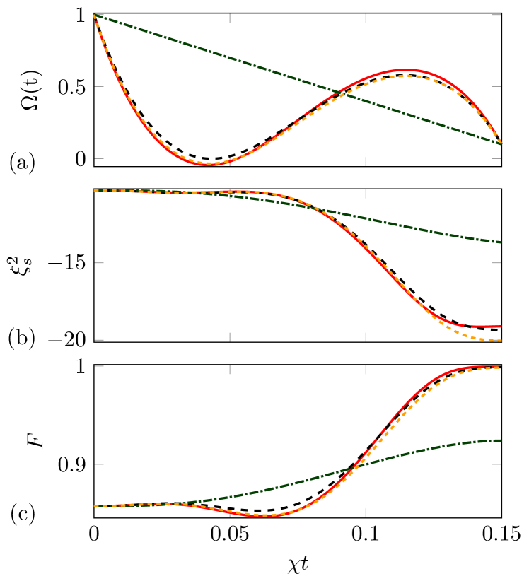
Figure 2: Time evolution of (a) control function $\Omega(t)$, (b) coherent squeezing $\xi_{S}^{2}(t)$ in dB, (d) fidelity $F(t)$. Enhanced STA ($\Omega_{e}$: red, solid lines), improved STA ($\Omega_{2}$, orange,small dashed lines), first STA scheme ($\Omega_{1}$, black, dashed lines) and as a reference linear adiabatic scheme ($\Omega_{ad}$, green, dashed-dotted lines). The parameter values used are $N=50$, $\chi t_{f}=0.15$, $\Lambda_{0}=10$, $\Omega_{f}/\Omega_{0}=0.1$.

As an example, Fig. 2 shows the time evolution of different quantifies with $N=50$ particles and the final time $\chi t_{f}=0.15$. In detail, in Fig. 2(a) we can see the different control functions. We compare here the adiabatic control $\Omega_{ad}(t)$, original, the STA scheme $\Omega_{1}(t)$, the improved STA scheme $\Omega_{2}(t)$ and the eSTA scheme $\Omega_{e}(t)$.

The remaining figures are the time evolution of the coherent spin-squeezing parameter $\xi_{S}^{2}$ (9) expressed in dB [Fig. 2(b)] as well as the fidelity $F$ [Fig. 2(c)] when the four different control functions are applied. We can see that the improved STA scheme $\Omega_{2}$ gives already higher fidelity than the first STA scheme $\Omega_{1}$. The eSTA scheme $\Omega_{e}$ gives even higher fidelity than the improved STA scheme $\Omega_{2}$, without compromising the squeezing.

We want to examine this in more detail and therefore we plot the fidelity for different final times $t_{f}$ and for the different control schemes ($\Omega_{ad},\Omega_{1},\Omega_{2},\Omega_{e}$). The results are summarized in Fig. 3, for $N=50$, $N=200$ and $N=400$ particles. From the figures, we can see that generally the eSTA protocol outperforms its STA counterpart, especially for shorter final times $\chi t_{f}$. Another important feature that we like to point out is the fact that the improved version of the STA protocol, characterised by $\Omega_{2}$ is consistently better than the non improved STA $\Omega_{1}$. This result shows improvements can be achieved even without applying the eSTA formalism, but using the correct boundary conditions for the system under consideration. Moreover, the fidelity of the three protocols tend to converge to 1 as the final time increases. It is also interesting to see how increasing the interaction strength $\chi$ (i.e. moving up a column in the figure grid), corresponds to an improvement in the performance of the protocols. This can be explained by the fact that the approximation $\Lambda_{0}>>1$ gets increasingly more accurate as the value of $\Lambda_{0}$ grows. On the other hand, we can see how keeping constant the interaction strength and increasing the number of particles (this amounts to move along a row on the figure grid) does not change the overall behaviour of the fidelity, only the intrinsic time of the system scales with the number of particles.

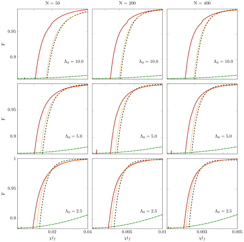
Figure 3: Fidelities $F$ versus final time $t_{f}$ for the different control schemes: eSTA ($\Omega_{e}$: red, solid lines), improved STA ($\Omega_{2}$, orange, small dashed lines), first STA scheme ($\Omega_{1}$, black, dashed lines) and as a reference linear adiabatic scheme ($\Omega_{ad}$, green, dashed-dotted lines) with different particle numbers $N=50$ (left column), $N=200$ (middle column), $N=400$ (right column) as well as different initial values of $\Lambda_{0}$ resp. $\Omega_{0}=\chi N/\Lambda_{0}$: $\Lambda_{0}=10.0$ (first row), $\Lambda_{0}=5.0$ (second row), $\Lambda_{0}=2.5$ (third row). $\Omega_{f}/\Omega_{0}=\Lambda_{0}/\Lambda_{f}=1/10$.

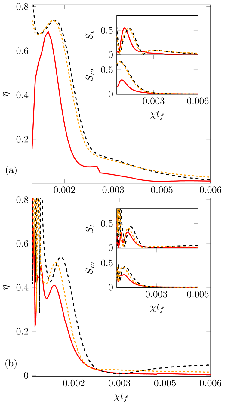
Figure 4: Imperfection $\eta$ (outer figures); sensitivity $S_{m}$ for systematic amplitude error and sensitivity $S_{t}$ for systematic time-shift (insets). Enhanced STA ($\Omega_{e}$: red, solid lines), improved STA ($\Omega_{2}$, orange,small dashed lines) and first STA scheme ($\Omega_{1}$, black, dashed lines). $N=400$, (a) $\Lambda_{0}=2.5$, (b) $\Lambda_{0}=10$.

IV.2 Robustness of the STA- and eSTA-based control schemes

It is important to ensure that a control scheme does not only provide high fidelity but that it is also robust against errors. Therefore, we will now compare the robustness of the above control schemes against systematic errors, i.e. an unknown, constant error in the experimental setup. First, we consider a systematic error in the amplitude of the control function $\Omega(t)$ of the form $\Omega_{\delta,m}(t)=(1+\delta)\Omega(t)$ for $t\in[0,t_{f}]$ and for an unknown constant value of $\delta$. To quantify the sensitivity of the control scheme to systematic errors of this type, we evaluate numerically the sensitivity

$$S_{m}=\left|\frac{\partial F}{\partial\delta}\right|_{\delta=0}\>.$$ (29)

for each control scheme used. Note that the lower this sensitivity is, the more stable the protocol is. The obtained results for $S_{m}$ are displayed in Fig. 4 (upper inset) for $N=400$ and $\Lambda_{0}=5$ [see the upper inset of Fig. 4(a)] and $\Lambda_{0}=20$ [see the upper inset of Fig. 4(b)].

We also consider a second type of systematic error. This second case is the systematic error in the time of the control function $\Omega(t)$ of the form $\Omega_{\bar{\delta},t}(t)=\Omega(t+t_{f}\bar{\delta})$ for $t+t_{f}\bar{\delta}\in[0,t_{f}]$ and $\Omega_{\bar{\delta},t}=\Omega(t)$ otherwise. Similar to Eq. (30) above, we compute numerically the corresponding systematic error sensitivity

$$S_{t}=\left|\frac{\partial F}{\partial\bar{\delta}}\right|_{\bar{\delta}=0}\>.$$ (30)

The results obtained for $S_{t}$ are illustrated in Fig. 4 (lower inset) for $N=400$ and $\Lambda_{0}=5$ [see the lower inset of Fig. 4(a)] and $\Lambda_{0}=20$ [see the lower inset of Fig. 4(b)].

It is pertinent to also incorporate the fidelity and these sensitivities in a single figure of merit, which will be referred to as imperfection in what follows. This quantity is given by

$$\eta=\sqrt{(1-F)^{2}+S_{m}^{2}+S_{t}^{2}}\>,$$ (31)

where $F$ is the fidelity and $S_{m},S_{t}$ are the sensitivities defined above. Therefore, a small value of $\eta$ corresponds to low infidelity (i.e. high fidelity) and small sensitivities (i.e. high degree of robustness) to the both systematic errors, i.e. the lower the value of $\eta$, the better the control scheme. The results are illustrated in Fig. 4 (outer figures) for $N=400$ and $\Lambda_{0}=2.5$ [see Fig. 4(a)] and $\Lambda_{0}=10$ [see Fig. 4(b)]. What can be inferred from these results is that the best performance is achieved using the eSTA method.

IV.3 Comparison of various approaches for engineering spin-squeezed states in internal BJJs

In order to quantitatively assess our proposed eSTA-based scheme for engineering spin-squeezed states in internal BJJs, it is pertinent to compare the achievable spin squeezing obtained using this scheme with the ones obtained with previously known schemes Gro (b); Rie .. Generally speaking, for different total evolution times $t_{f}$, the eSTA-based scheme slightly outperforms its STA-based counterpart in terms of achievable spin squeezing, as quantified by the previously introduced parameters $\xi^{2}_{S}$ and $\xi^{2}_{N}$ [cf. Sec. II.2]. However, the primary advantage of the eSTA approach, which makes it much more powerful than STA, lies in its superior robustness against systematic errors.

For the sake of illustration, it is instructive to consider a system with $N=400$ particles, with the same value of the nonlinear-coupling strength $\chi=2\pi\times 0.063$ Hz used in an experimental study of Ref. Gro (b). While in Gro (b) the linear-coupling strength $\Omega$ was fixed to the constant value $\Omega=2\pi\times 2$ Hz – leading to a ratio $\chi/\Omega=0.03$ – in the present work we consider a significant variation of the linear-coupling strength with time. As a result of this variation, the control parameter $\Lambda(t)$ is changed from $\Lambda(0)/N=\chi/\Omega(0)=1/160$ to $\Lambda(t_{f})/N=\chi/\Omega(t_{f})=1/40$ ($N=400$); in this manner, we demonstrate that our proposed eSTA-based scheme for the generation of spin-squeezed states is applicable even far away from the adiabatic regime. Importantly, the total squeezed-state preparation time that we obtain here [cf. Fig. 3] is then $t_{f}=0.006\>\chi^{-1}\approx\>15$ ms for the largest value of $\Lambda_{0}/N$ used ($1/40$) and $t_{f}=0.0015\>\chi^{-1}\approx\>3.75$ ms for its smallest value ($1/160$); the longer of these two times is around $25\%$ shorter than the squeezed-state preparation time of $20$ ms found in Ref. Gro (b).

Our numerical calculations indicate that the two schemes for engineering spin-squeezed states – STA- and eSTA-based ones – are quite comparable in terms of of achievable spin squeezing. For example, in a system with $N=50$ particles and $\Lambda_{0}/N=0.2$ the eSTA control scheme allows one to attain a value of $\xi_{S}^{2}<-18$ dB while the adiabatic scheme only yields a value of $\xi_{S}^{2}>-14$ dB, see Fig. 2.

The effects of the application of the eSTA protocol get increasingly less prominent as the number of particles increases. For instance, for a system with $N=400$ particles, $t_{f}=0.1/\chi$ and $\Lambda_{0}/N=10$ both the eSTA-based scheme and the STA-based one, yield $\xi_{S}^{2}=-19$ dB. It is useful to recall that the eSTA protocol is designed with the aim to maximize the fidelity of the system. The fact that the squeezing obtained via eSTA protocol is comparable, if not better, than the one obtained using the STA approach is another argument in favor of eSTA.

On the other hand, the eSTA-based protocol has a lower sensitivity $S_{m}$ than the STA and improved STA protocols against systematic errors as it can straightforwardly be inferred from the sensitivities shown in the insets of Fig. 4; thus, the eSTA scheme is significantly less sensitive (i.e. more robust) to systematic errors in the amplitude of $\Omega$ than the STA-based one. In the insets of the same figure, similar behavior is found for the systematic error pertaining to the timing of the control scheme $\Omega$; for the above choice of parameter values, the sensitivity $S_{t}$ is again lower for the eSTA scheme than for the STA scheme and its improved version.

The observed superiority of the eSTA-based approach over its STA-based counterpart in the system under consideration is more prominent for shorter times $t_{f}$. Importantly, this superiority of the eSTA-based approach is not dependent upon the particle number; it persists even for a system with several hundred (or even thousand) particles. The fact that the eSTA method allows one to attain a rather strong spin squeezing in internal BJJs – being at the same time much more robust against systematic errors than STA – makes this method a highly promising candidate for the experimental realization of spin-squeezed states in this type of systems.

The TNT dynamics of spin squeezing in internal BJJs has so far been demonstrated experimentally by abruptly switching the nonlinear coupling to a finite value (i.e. by performing a nonlinear-coupling quench) in the presence of constant linear coupling $\Omega$ Muessel+:15 ; in this case a Feshbach resonance was used as an enabling physical mechanism for increasing the nonlinear coupling strength. This investigated scenario of TNT dynamics, with a fixed ratio of the nonlinear- and linear coupling strenghts, has already also been shown – in the absence of decoherence and losses – to be locally optimal as far as the generation of spin squeezing is concerned Sor (c). However, there are several reasons that make it quite plausible to expect that in the realistic experimental scenario (i.e. in the presence of decoherence and losses, as well as various experimental imperfections) the eSTA-based approach proposed here could yield comparable – or, perhaps, even better – results. To begin with, the eSTA method Whitty+:20 has already been demonstrated to yield results approaching the relevant quantum speed limits in some other quantum-control problems Hau (b); Whitty+:22 . In addition, the extraordinary robustness to various experimental imperfections that is inherent to the eSTA method – compared to its parent STA methods and other control approaches – also favors our envisioned approach. Finally, our scheme may turn out to be more robust to atomic losses (most prominently, two-body spin-relaxation losses for $F=2$ hyperfine states); in the existing experimental realization Muessel+:15 , for the same range of particle numbers as discussed here the combined effect of two- and three-body losses led to a substantial (above $20\%$) decrease of the maximal achievable spin squeezing.

V Summary and conclusions

In summary, in this paper we revisited – from the quantum-control perspective – the problem of robust, time-efficient engineering of spin-squeezed states in internal bosonic Josephson junctions with a time-dependent linear (Rabi) coupling. Unlike earlier studies in which this state-engineering problem was treated using adiabatic- or STA methods, we addressed it here using the recently proposed eSTA approach. Taking the standard Lipkin-Meshkov-Glick-type Hamiltonian of this system – which in addition to the standard one-axis twisting term includes the transverse-field (turning) term – as our point of departure, we designed a robust eSTA-based state-preparation scheme. To characterize the twist-and-turn-type quantum dynamics underlying the preparation of spin-squeezed states in this system in a quantitative fashion, we computed the corresponding (time-dependent) target-state fidelity. We also evaluated two of the most relevant figures of merit of spin squeezing – namely, the coherent spin-squeezing- and number-squeezing parameters – in a broad range of the relevant parameters of the system.

Importantly, we showed that our eSTA-based scheme for engineering spin-squeezed states outperforms – in terms of achievable state fidelities and the attendant state-preparation times – not only the previously proposed STA protocols, but also their improved version; this superiority of our eSTA-based approach is not limited only to relatively small particle numbers, but persists even in systems containing several hundred particles. In particular, we demonstrated that the increased robustness of the eSTA approach, compared to its parent STA method, renders our proposed state-preparation scheme more amenable to experimental realizations than the previously suggested schemes for engineering spin-squeezed states in bosonic Josephson junctions. In order to further facilitate the envisioned experimental realizations, a future theoretical work should be devoted to discussing other possible decoherence effects (other than those already discussed here) in this system, most prominently that of atomic losses Sinatra+:12 .