Specific Wasserstein divergence between continuous martingales

Abstract.

Defining a divergence between the laws of continuous martingales is a delicate task, owing to the fact that these laws tend to be singular to each other. An important idea, put forward by N. Gantert in [31], is to instead consider a scaling limit of the relative entropy between such continuous martingales sampled over a finite time grid. This gives rise to the concept of specific relative entropy. In order to develop a general theory of divergences between continuous martingales, it is only natural to replace the role of the relative entropy in this construction by a different notion of discrepancy between finite dimensional probability distributions. In the present work we take a first step in this direction, taking a power $p$ of the Wasserstein distance instead of the relative entropy. We call the newly obtained scaling limit the specific $p$-Wasserstein divergence.

In our first main result we prove that the specific $p$-Wasserstein divergence is well-defined, and exhibit an explicit expression for it in terms of the quadratic variations of the martingales involved. This is obtained under vastly weaker assumptions than the corresponding results for the specific relative entropy. Next we illustrate the usefulness of the concept, by considering the problem of optimizing the specific $p$-Wasserstein divergence over the set of win-martingales. In our second main result we characterize the solution of this optimization problem for all $p>0$ and, somewhat surprisingly, we single out the case $p=1/2$ as the one with the best probabilistic properties. For instance, the optimal martingale in this case is very explicit and can be connected, through a space transformation, to the solution of a variant of the Schrödinger problem.

1. Introduction

The aim of this paper is to introduce a novel notion of divergence between continuous martingales, and thereafter to fully study and solve divergence optimization problems over the set of win martingales (used as models for prediction markets [3]).

Identifying two real-valued continuous martingales as probability measures $\mathbb{Q},\mathbb{P}$ on the continuous path space

$$C([0,1];\mathbb{R}),$$

a natural choice for divergence would be the relative entropy

$$H(\mathbb{Q}||\mathbb{P})=\int\frac{d\mathbb{Q}}{d\mathbb{P}}\,\log\big{(}\frac{d\mathbb{Q}}{d\mathbb{P}}\big{)}\,d\mathbb{P},$$

or its generalization, the $f$-divergence $\int f(\frac{d\mathbb{Q}}{d\mathbb{P}})\,d\mathbb{P}$. This naive approach leads to an immediate difficulty, namely, that the laws of continuous martingales tend to be singular to each other and hence have a trivial divergence in the above sense. As an example, the reader can consider $\mathbb{Q},\mathbb{P}$ to be respectively the laws of Brownian motion and two times the Brownian motion, and check that these measures are concentrated on disjoint sets.

A natural approach to circumvent this difficulty is to rather discretize the martingales in time, compare them at the discrete-time level, and then consider a (scaling) limit in which the time mesh-size goes to zero. This approach was introduced by Gantert in [31], and more recently refined by Föllmer in [28], leading to the notion of specific relative entropy between continuous martingales. The key in that construction is to use the conventional relative entropy when comparing the laws of the time-discretized martingales. In this article we introduce and study the specific Wasserstein divergence, obtained by considering a power of the Wasserstein distance instead of the relative entropy in the aforementioned scaling limit. This is hence a first step towards a general theory of divergences between continuous martingales.

1.1. Specific Wasserstein divergence

Denote throughout by $\mathcal{P}(\mathcal{X})$ the space of probability measures on a Polish space $\mathcal{X}$.

Given a function $F:\mathcal{P}(\mathbb{R})\times\mathcal{P}(\mathbb{R})\to\mathbb{R}_{+}$ which only vanishes on the diagonal, we may interpret $D_{F}^{1}(\mu,\nu):=F(\mu,\nu)$ as the discrepancy between $\mu$ and $\nu\in\mathcal{P}(\mathbb{R})$. Inductively, after having defined $D_{F}^{N-1}:\mathcal{P}(\mathbb{R}^{N-1})\times\mathcal{P}(\mathbb{R}^{N-1})\to\mathbb{R}_{+}$, a discrepancy functional between elements in $\mathcal{P}(\mathbb{R}^{N-1})$, then a natural choice for a discrepancy functional between elements in $\mathcal{P}(\mathbb{R}^{N})$ is given by

$$D_{F}^{N}(\mathbb{Q}||\mathbb{P}):=D_{F}^{N-1}(\mathbb{Q}_{1:N-1}||\mathbb{P}_{1:N-1})+\int F(\mathbb{Q}_{N}^{x_{1:N-1}},\mathbb{P}_{N}^{x_{1:N-1}})\,d\mathbb{Q}_{1:N-1}(x_{1:N-1}),$$ (1.1)

where $\mathbb{Q}_{1:N-1}$ is the projection of $\mathbb{Q}$ on the first $N-1$ coordinates, $x_{1:N-1}=(x_{1},\dotso,x_{N-1})\in\mathbb{R}^{N-1}$, $\mathbb{Q}_{N}^{x_{1:N-1}}$ is the conditional law of the $N$-th marginal given the previous trajectory $x_{1:N-1}$, with similar notations for $\mathbb{P}_{1:N-1}$ and $\mathbb{P}_{N}^{x_{1:N-1}}$.

If now $\mathbb{Q},\mathbb{P}\in\mathcal{P}(C([0,1];\mathbb{R}))$, a natural choice for a discrepancy functional between $\mathbb{Q}$ and $\mathbb{P}$ is to take

$$\lim\limits_{N\to\infty}c^{F}_{N}D^{N}_{F}((\mathbb{Q})_{N}||(\mathbb{P})_{N}),$$

assuming that the limit exists and that a universal scaling sequence $\{c^{F}_{N}\}_{N}\subseteq\mathbb{R}_{+}$ has been found. Here and throughout we use the notation $(\mathbb{Q})_{N}$ for the push-forward (i.e., image measure) of $\mathbb{Q}$ under the map

$$C([0,1];\mathbb{R})\ni\omega\mapsto(\omega_{1/N},\omega_{2/N},\dots,\omega_{N/N}),$$

and likewise for $(\mathbb{P})_{N}$.

We remark that (1.1) is akin to the time consistency property in the theory of dynamic risk measures (see Remark 2.4 below), and is very natural given the temporal structure of processes like martingales. Taking $F$ to be the relative entropy $H$, the construction described so far gives rise (with $c^{F}_{N}=N^{-1}$) to the specific relative entropy. Thus the specific relative entropy can be understood as the rate of increase of the relative entropy as the number of marginals taken into account increases.

In this paper, we will be concerned with the case

$$F=\mathcal{W}_{1}^{p},$$

where $\mathcal{W}_{1}$ is the celebrated Wasserstein-$1$ distance and $p$ is any positive real number. We call the resulting object the specific $p$-Wasserstein divergence (though sometimes we omit to mention the parameter $p$), and denote it by $\mathcal{SW}_{p}$. Moreover, we will only be concerned with continuous martingale laws throughout. As a side note, we remark that taking a different Wasserstein distance than $\mathcal{W}_{1}$ would change very little the results in this paper.

We proceed to describe our first main result: Suppose $\mathbb{Q}$ is the law of a continuous martingale starting wlog. at 0 and admitting an absolutely continuous quadratic variation with density denoted by $\sigma^{2}$. Suppose that $\mathbb{P}$ is the law of standard Brownian motion. In Theorem 2.9 we obtain the existence of the specific Wasserstein divergence together with its explicit formula

$$\mathcal{SW}_{p}(\mathbb{Q}||\mathbb{P}):= \lim_{\begin{subarray}{c}N=2^{n}\\ n\to\infty\end{subarray}}N^{p/2-1}D_{\mathcal{W}}^{N,p}((\mathbb{Q})_{N}||(\mathbb{P})_{N})=(2/\pi)^{p/2}\mathbb{E}_{\mathbb{Q}}\left[\int_{0}^{1}\left(|\sigma_{t}|-1\right)^{p}\,dt\right].$$

In fact, in Theorem 2.9 we can allow the law $\mathbb{P}$ to be more general than the Wiener measure, e.g. it can come from the law of a martingale diffusion with a well-behaved volatility coefficient. One notable aspect of this result is that the assumptions needed are vastly weaker than the ones needed for the corresponding result in the case of the specific relative entropy. In particular, we can handle the situation where $\mathbb{P}$ is the constant martingale (i.e., a Brownian motion with zero volatility), and more generally, certain cases where $(\mathbb{Q})_{N}$ and $(\mathbb{P})_{N}$ may be singular to each other for every $N$. We consider this result a first step towards building a general theory of divergences between continuous martingales, since unlike the case of the specific relative entropy, the construction here gives a whole family of divergences.

Related to the above main result, we recover in Proposition 2.16 a functional inequality by Föllmer [28] concerning (in our terminology) the specific Wasserstein divergence, specific relative entropy, and an adapted Wasserstein distance. Our proof method is based on Theorem 2.9 and different from the original approach by this author.

1.2. Optimization over win-martingales

The main application of the concept of specific Wasserstein divergence that we want to put forward in this paper, concerns a problem of optimization over the set of win-martingales. A continuous time martingale $(X_{t})$ over time $t\in[0,1]$ is called a win-martingale if it starts with a deterministic position $X_{0}=x_{0}\in(0,1)$ and ends up at time 1 on either $0$ or $1$. In other words, it transports $\delta_{x_{0}}$ at time $0$ to $Bernoulli(x_{0})$ at time $1$. Such martingales have been proposed as models of prediction markets (cf. [3]) and optimization problems over the set of win-martingales were proposed by Aldous [2].

Given a fixed initial position $x_{0}\in(0,1)$ and $p>0$, our aim is to optimize the specific Wasserstein divergence $\mathcal{SW}_{p}(\mathbb{Q}||\mathbb{P}_{\delta})$ among all continuous win-martingales $\mathbb{Q}$ started at $x_{0}$ and admitting an absolutely continuous quadratic variation, whereby $\mathbb{P}_{\delta}$ denotes the constant martingale. More specifically, we maximize $\mathcal{SW}_{p}(\mathbb{Q}||\mathbb{P}_{\delta})$ for $p\in(0,2)$ and minimize $\mathcal{SW}_{p}(\mathbb{Q}||\mathbb{P}_{\delta})$ for $p\in(2,\infty)$. These optimization problems are related to the one in [7], wherein the specific relative entropy with respect to standard Brownian motion is minimized over this set of martingales. Similarly to this reference, we employ first order conditions to characterize in Proposition 3.3, via ordinary differential equations, the (Markovian) volatility coefficient of a candidate optimal martingale. Then, in Section 4, the optimality of the candidate is verified by making use of the associated HJB equation and stochastic analysis arguments. Hence we obtain semi-explicit solutions for a whole family of continuous-time martingale optimal transport problems (which cannot be transformed into an Skorokhod Embedding Problem), usually considered a difficult task.

We identify two cases where the solution to our problem is fully explicit. One is for $p=1$, where the solution is a so-called Bass martingale (see [8, 10]). As this object is well studied we do not explore this case in any detail. The fully novel case is $p=1/2$. In this setting the unique optimal win martingale solves the SDE

$$dM_{t}=\sqrt{\frac{2}{1-t}}M_{t}(1-M_{t})\,dB_{t}.$$

In order to provide some intuition, we provide some numerical simulations of the Bass martingale and $(M_{t})$. The reader may notice that the former tends to explore the space relatively faster than the latter. Indeed Lemma 3.6 below justifies that for each moment of time $t\in[0,1]$, the distribution of the Bass martingale is greater than that of $M_{t}$ in the sense of convex order.

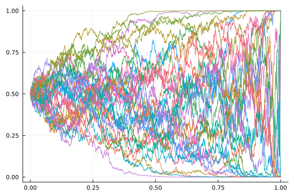
Figure 1. Simulations of Bass martingales ($p=1$).

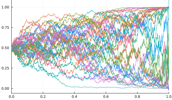
Figure 2. Simulations of $(M_{t})$, i.e. case $p=1/2$.

If we stretch the time-index set from $[0,1]$ to $[0,\infty)$ in a natural way, the time-changed martingale $Y_{t}:=M_{1-e^{-t/2}}$ admits the more amenable form

$$dY_{t}=Y_{t}(1-Y_{t})\,dW_{t},$$

with $W$ a suitable Brownian motion. In this form, it can be readily interpreted in terms of filtering theory. Indeed, $Y_{t}$ is precisely the conditional probability of the drift being equal to $1$ for a Brownian motion with an unobservable drift which can be either 0 or 1. Moreover the marginal distributions of $M$ and $Y$ are fully explicit and simple to describe. This is in stark contrast to the situation in [7].

If we then perform a change of space-scale

$$C_{t}:=\log(Y_{t}/(1-Y_{t})),$$

so that the resulting process has unit volatility coefficient, it turns out that this process satisfies the SDE

$$dC_{t}=\frac{1}{2}\tanh\left(\frac{C_{t}}{2}\right)dt+dW_{t}.$$

This process can also be interpreted in a number of interesting ways. For instance the marginal laws of $C$ are a mixture between the marginal laws of a drifted Brownian motion with drift $\pm 1/2$. More interestingly, we have the following result, where we denote by $\mathbb{W}^{0}_{T,x}$ the law of the Brownian bridge from 0 at time 0 to $x$ at time $T$, and we define $\mathbb{W}_{T,\pm T/2}^{0}:=\frac{1}{2}\left(\mathbb{W}_{T,T/2}^{0}+\mathbb{W}_{T,-T/2}^{0}\right)$:

For every $t\in\mathbb{R}_{+}$, the law $\mathbb{W}_{T,\pm T/2}^{0}$ restricted to $[0,t]$ converges as $T\to\infty$ to the law of $C$ restricted to $[0,t]$.

This result, which we formalize in Theorem 5.4, says that $C$ is precisely the law of Brownian motion $W$ conditioned on the event $W_{T}=\pm T/2$ as $T\to\infty$. In other words, $C$ is a solution (more precisely, a limit of solutions) to the celebrated Schrödinger problem (see [43]). To the authors’ best knowledge, this is the first instance that a solution to a continuous martingale transport problem has been naturally connected to the solution of a likewise continuous Schrödinger problem.

1.3. Connections to the literature

The specific relative entropy was introduced and interpreted as a rate function by Gantert [31]. More recently [12] obtained an explicit formula for this quantity (between time-homogeneous Markov martingales), and Föllmer [28] extended Gantert’s results and established a Talagrand-type inequality between semimartingale laws using this object. In [7] the specific relative entropy was used to solve an open question by Aldous (see [33] for an alternative point of view and solution).

The adapted Wasserstein distance, appearing in the aforementioned Talagrand-type inequality by Föllmer, is a metric between stochastic processes that incorporates their temporal structure; see [6, 9, 13, 42] among others.

Win-martingales have been proposed as models for prediction markets (cf. [3]), and optimization problems over the set of win-martingales were proposed by Aldous [2] in connection to the aforementioned open question. Such optimization problems are particular instances of martingale optimal transport, a subject that has been extensively studied in the recent years. Following [36, 16, 22, 30] martingale versions of the classical transport problem (see e.g. [57, 58, 52, 27] for recent monographs) are often considered due to applications in mathematical finance but admit further applications, e.g. to the Skorokhod problem [15, 19]. In analogy to classical optimal transport, necessary and sufficient conditions for optimality have been established for martingale transport (MOT) problems in discrete time ([18, 20]) but not so much is known for the continuous time problem. Notable exceptions are [38, 55, 8, 10, 7, 33, 45, 34].

The Schrödinger problem has its origin in [53, 54]. In a nutshell, it asks for the most likely evolution for a large system of particles given initial and terminal configurations. By they theory of large deviation, this amounts to an entropy minimization problem. If the initial configuration is a point mass and the particles are Markovian, its solution is a Markov bridge [44]. We refer to Léonard’s survey [43] for a historical account and to the more contemporary articles [4, 21, 23, 24, 49] for recent contributions.

Finally we mention the work of Lacker [41], extended e.g. in [11, 26], wherein the idea of considering a scaling limit of problems in ever higher dimension is also considered. This is more related to a large deviations principle for a particle system whose size goes to infinity, rather than to our framework of a single process that we examine at ever finer resolution.

2. Specific Wasserstein divergence between martingales

2.1. Specific Wasserstein divergence

For Borel probability measures $\mu,\nu\in\mathcal{P}_{1}(\mathcal{X})$ on a metric space $(\mathcal{X},d)$ we define their $1$-Wasserstein distance

$$\mathcal{W}_{1}(\mu,\nu):=\inf_{\pi\in\Pi(\mu,\nu)}\int d(x,y)\,d\pi(x,y),$$

whereby $\mathcal{P}_{1}(\mathcal{X}):=\{\rho\in\mathcal{P}(\mathcal{X}):\,\int d(x,x_{0})\,d\rho(x)<\infty,\text{ some }x_{0}\}$ and $\Pi(\mu,\nu)$ stands for the set of probability measures on $\mathcal{X}\times\mathcal{X}$ with first marginal $\mu$ and second marginal $\nu$. See [57, Chapter 7] for background. In case $\mathcal{X}$ is Euclidean space we will always take $d$ to be the metric associated to the Euclidean norm.

In order to define a time-consistent divergence on $\mathcal{P}_{1}(\mathbb{R}^{N})$, with the aforementioned one-dimensional Wasserstein distance as a building block, we proceed inductively. We shall employ the following notation throughout: If $x\in\mathbb{R}^{N}$, then $x_{i:j}:=(x_{i},x_{i+1},\dots,x_{j})$ for $i<j$ and $x_{i:i}=x_{i}$. Likewise if $\mathbb{P}\in\mathcal{P}(\mathbb{R}^{N})$, then $\mathbb{P}_{i:j}$ is the law of $x_{i:j}$ under $\mathbb{P}$ and we denote $\mathbb{P}_{i}:=\mathbb{P}_{i:i}$. We write $\mathbb{P}^{x_{1:i-1}}_{i}$ for the conditional law of $x_{i}$ under $\mathbb{P}$ given the information of $x_{1:i-1}$, and use the convention $\mathbb{P}^{x_{1:0}}_{1}:=\mathbb{P}_{1}$.

We fix $p>0$ and define:

Definition 2.1.

Suppose $\mathbb{Q},\mathbb{P}\in\mathcal{P}_{1}(\mathbb{R})$, then $D_{\mathcal{W}}^{1,p}(\mathbb{Q}||\mathbb{P}):=\mathcal{W}_{1}^{p}(\mathbb{Q},\mathbb{P})$. For $N>1$, supposing that $\mathbb{Q},\mathbb{P}\in\mathcal{P}_{1}(\mathbb{R}^{N})$ are such that $P^{x_{1:i-1}}_{i}$ is well-defined $\mathbb{Q}_{1:i-1}$-a.s. for each $i\in\{1,\dots,N\}$, then we define inductively

$$D_{\mathcal{W}}^{N,p}(\mathbb{Q}||\mathbb{P}):=D_{\mathcal{W}}^{N-1,p}(\mathbb{Q}_{1:N-1}||\mathbb{P}_{1:N-1})+\int\mathcal{W}_{1}^{p}(\mathbb{Q}^{x_{1:N-1}}_{N},\mathbb{P}^{x_{1:N-1}}_{N})\,d\mathbb{Q}_{1:N-1}(x_{1:N-1}).$$

Unravelling the induction, we clearly have the equivalent expression

$$D_{\mathcal{W}}^{N,p}(\mathbb{Q}||\mathbb{P})=\int_{\mathbb{R}^{N}}\left[\sum_{i=1}^{N}\mathcal{W}_{1}^{p}(\mathbb{Q}^{x_{1:i-1}}_{i},\mathbb{P}^{x_{1:i-1}}_{i})\right]d\mathbb{Q}(x).$$

Remark 2.2.

In the definition of $D_{\mathcal{W}}^{N,p}(\mathbb{Q}||\mathbb{P})$, the assumption that $\mathbb{P}^{x_{1:i-1}}_{i}$ is well-defined $\mathbb{Q}_{1:i-1}$-a.s. is necessary to integrate $\mathcal{W}_{1}^{p}(\mathbb{Q}^{x_{1:i-1}}_{i},\mathbb{P}^{x_{1:i-1}}_{i})$ with respect to $\mathbb{Q}_{1:i-1}$. One sufficient condition for this is that $\mathbb{Q}_{1:i-1}\ll\mathbb{P}_{1:i-1}$ for any $i=1,\dotso,N$. Another sufficient condition is when $\mathbb{P}$ is the law of a discrete-time Markov process which is uniquely defined by transition kernels $\{\mathbb{P}^{x_{i-1}}_{i}:\,i=1,\dotso,N,x_{i-1}\in\mathbb{R}\}$ which are defined everywhere.

Remark 2.3.

For $p\geq 1$, thanks to the convexity of $\mathbb{Q}\mapsto\mathcal{W}_{1}(\mathbb{Q},\mathbb{P})$, it follows that $D^{N,p}_{\mathcal{W}}(\mathbb{Q},\mathbb{P})$ is also convex in $\mathbb{Q}$. To see this, take wlog. $N=2$ and two probability distribution $\mathbb{Q},\tilde{\mathbb{Q}}\in\mathcal{P}_{1}(\mathbb{R}^{2})$. Letting $t\in[0,1]$, it can be seen that $t\mathbb{Q}+(1-t)\tilde{\mathbb{Q}}$ has the disintegration

$$\left(t\mathbb{Q}_{1}+(1-t)\tilde{\mathbb{Q}}_{1}\right)\otimes\left(\frac{t\mathbb{Q}_{2}^{x_{1}}\,d\mathbb{Q}_{1}(x_{1})+(1-t)\tilde{\mathbb{Q}}_{2}^{x_{1}}\,d\tilde{\mathbb{Q}}_{1}(x_{1})}{t\,d\mathbb{Q}_{1}(x_{1})+(1-t)\,d\tilde{\mathbb{Q}}_{1}(x_{1})}\right),$$

and hence

$$\int\mathcal{W}_{1}^{p}\left(\frac{t\mathbb{Q}_{2}^{x_{1}}\,d\mathbb{Q}_{1}(x_{1})+(1-t)\tilde{\mathbb{Q}}_{2}^{x_{1}}\,d\tilde{\mathbb{Q}}_{1}(x_{1})}{t\,d\mathbb{Q}_{1}(x_{1})+(1-t)\,d\tilde{\mathbb{Q}}_{1}(x_{1})},\mathbb{P}^{x_{1}}_{2}\right)\,d(t\mathbb{Q}_{1}(x_{1})+(1-t)\tilde{\mathbb{Q}}_{1}(x_{1}))$$

$$\leq\int\frac{t\,d\mathbb{Q}_{1}(x_{1})}{t\,d\mathbb{Q}_{1}(x_{1})+(1-t)\,d\tilde{\mathbb{Q}}_{1}(x_{1})}\mathcal{W}_{1}^{p}(\mathbb{Q}_{2}^{x_{1}}||\mathbb{P}^{x_{1}}_{2})\,d(t\mathbb{Q}_{1}(x_{1})+(1-t)\tilde{\mathbb{Q}}_{1}(x_{1}))$$

$$\quad+\int\frac{(1-t)\,d\tilde{\mathbb{Q}}_{1}(x_{1})}{t\,d\mathbb{Q}_{1}(x_{1})+(1-t)\,d\tilde{\mathbb{Q}}_{1}(x_{1})}\mathcal{W}_{1}^{p}(\tilde{\mathbb{Q}}_{2}^{x_{1}}||\mathbb{P}^{x_{1}}_{2})\,d(t\mathbb{Q}_{1}(x_{1})+(1-t)\tilde{\mathbb{Q}}_{1}(x_{1}))$$

$$=t\int\mathcal{W}_{p}^{p}(\mathbb{Q}_{2}^{x_{1}}||\mathbb{P}^{x_{1}}_{2})\,d\mathbb{Q}_{1}(x_{1})+(1-t)\int\mathcal{W}_{1}^{p}(\tilde{\mathbb{Q}}_{2}^{x_{1}}||\mathbb{P}^{x_{1}}_{2})\,d\tilde{\mathbb{Q}}_{1}(x_{1}).$$

In the computation above, the crucial point is the convexity of $\mathcal{W}_{1}$, or more precisely, of $\mathcal{W}_{1}^{p}$. This is also the case for $\mathcal{W}_{q}^{p}$ with $1\leq q\leq p$, with $\mathcal{W}_{q}$ denoting the $q$-Wasserstein distance. In order to keep the convexity of $D^{N,p}_{\mathcal{W}}$ for any $p\geq 1$ we choose in this work $q=1$ throughout, but we could have easily considered $\mathcal{W}_{q}$ instead of $\mathcal{W}_{1}$.

Remark 2.4.

The construction in Definition 2.1 is the exact analogue to the Bellman principle for the conditional penalty functions of dynamic convex risk measures; see [29, Theorem 4.5]. An example of the latter is the additive decomposition of the relative entropy.

In this article, we are interested in the divergence between the distributions of two continuous martingales taking real values. Hence we consider the classical Wiener space

$$\Omega:=C([0,1];\mathbb{R})$$

equipped with its natural Borel $\sigma$-algebra. We will denote throughout by $X$ the canonical process

$$X(\omega)=\omega,$$

and by $\langle X\rangle$ its quadratic variation process. Since we will only be dealing with martingale laws, we do not need to refer to a reference measure in order to define the quadratic variation; see Remark 2.10 for more details.

Inspired by [31], we define the specific Wasserstein divergence as a scaling limit of the finite dimensional discrepancy $D^{N,p}_{\mathcal{W}}$. For any $\mathbb{Q}\in\mathcal{P}(\Omega)$ and $N\in\mathbb{N}$, we denote by

$$(\mathbb{Q})_{N}\in\mathcal{P}(\mathbb{R}^{N}),$$

the law $\mathbb{Q}$ projected on the time-grid $\{k/N:k=1,\dots,N\}$.

Definition 2.5.

For any $\mathbb{Q},\mathbb{P}\in\mathcal{P}(\Omega)$, we define the specific $p$-Wasserstein divergence as

$$\mathcal{SW}_{p}(\mathbb{Q}||\mathbb{P}):=\liminf\limits_{\begin{subarray}{c}N=2^{n}\\ n\to\infty\end{subarray}}N^{p/2-1}D_{\mathcal{W}}^{N,p}((\mathbb{Q})_{N}||(\mathbb{P})_{N}),$$

if $D_{\mathcal{W}}^{N,p}((\mathbb{Q})_{N}||(\mathbb{P})_{N})$ is well-defined for all large enough $N=2^{n}$. Otherwise we set it to $+\infty$.

As the following lemma shows, if $\mathbb{W}^{\sigma}_{x_{0}}$ denotes the law of Brownian motion started at $x_{0}$ with instantaneous variance / volatility $\sigma^{2}>0$, then we have

$$D_{\mathcal{W}}^{N,p}((\mathbb{W}^{\tilde{\sigma}}_{x_{0}})_{N}||(\mathbb{W}^{\sigma}_{x_{0}})_{N}))=N^{-p/2+1}\mathcal{W}^{p}_{1}\left(\mathcal{N}(0,\tilde{\sigma}^{2}),\mathcal{N}(0,\sigma^{2})\right)=N^{-p/2+1}(2/\pi)^{p/2}(|\tilde{\sigma}|-|\sigma|)^{p}$$

and hence

$$\mathcal{SW}_{p}(\mathbb{W}^{\tilde{\sigma}}_{x_{0}}||\mathbb{W}^{\sigma}_{x_{0}})=(2/\pi)^{p/2}(|\tilde{\sigma}|-|\sigma|)^{p}.$$

Importantly, this suggests that the scaling factor $N^{-p/2+1}$ is the right one for our purposes.

We will need the following invariance property of the divergences $D^{N,p}_{\mathcal{W}}$:

Lemma 2.6.

Taking $T:\mathbb{R}^{N+1}\to\mathbb{R}^{N+1},\,(x_{1},x_{2},\dotso,x_{N+1})\mapsto(x_{1},x_{2}-x_{1},\dotso,x_{N+1}-x_{N})$ we have the following identity for any $\mathbb{Q},\mathbb{P}\in\mathcal{P}(\mathbb{R}^{N+1})$

$$D^{N+1,p}_{\mathcal{W}}(\mathbb{Q}||\mathbb{P})=D^{N+1,p}_{\mathcal{W}}(T(\mathbb{Q})||T(\mathbb{P})).$$

Proof.

Note that $T$ can also be considered as a map from $\mathbb{R}^{N}$ to $\mathbb{R}^{N}$ when restricted to the first $N$-coordinates, and hence $T(x_{1:N})$ is defined as $(x_{1},x_{2}-x_{1},\dotso,x_{N}-x_{N-1})$. Since $T$ is a bijection, it can be seen that

$$T(\mathbb{Q})_{N+1}^{T(x_{1:N})}=(x_{N+1}\mapsto x_{N+1}+x_{N})_{\#}\mathbb{Q}^{x_{1:N}}_{N+1},$$

and therefore due to the translation invariant property of Wasserstein distance,

$$\mathcal{W}_{1}^{p}(T(\mathbb{Q})^{T(x_{1:N})}_{N+1},T(\mathbb{P})^{T(x_{1:N})}_{N+1})=\mathcal{W}_{1}^{p}(\mathbb{Q}^{x_{1:N}}_{N+1},\mathbb{P}^{x_{1:N}}_{N+1}).$$

Now by change of measure,

$$\int\mathcal{W}_{1}^{p}(T(\mathbb{Q})^{x_{1:N}}_{N+1},T(\mathbb{P})^{x_{1:N}}_{N+1})\,dT(\mathbb{Q})_{1:N}(x_{1:N}) =\int\mathcal{W}_{1}^{p}(T(\mathbb{Q})^{T(x_{1:N})}_{N+1},T(\mathbb{P})^{T(x_{1:N})}_{N+1})\,d\mathbb{Q}_{1:N}(x_{1:N})$$

$$=\int\mathcal{W}_{1}^{p}(\mathbb{Q}^{x_{1:N}}_{N+1},\mathbb{P}^{x_{1:N}}_{N+1})\,d\mathbb{Q}_{1:N}(x_{1:N}),$$

and our claim follows by induction. ∎

We will now fix a particular choice of martingale measure, $\mathbb{P}$, playing the role of a reference measure. The reader can think of $\mathbb{P}$ as the law of Brownian motion, however the precise assumption that we need is as follows:

Assumptions 2.7.

Admit the existence of a jointly measurable function $\eta:[0,1]\times\mathbb{R}\to\mathbb{R}$, such that $x\mapsto\eta(t,x)$ is Lipschitz uniformly in $t$ and $\sup_{t\in[0,1]}|\eta(t,0)|<+\infty$. We denote by $\mathbb{P}^{x_{0}}$ the law of the solution of the SDE $dX_{t}=\eta(t,X_{t})dB_{t}$ starting from $x_{0}$, and if $x_{0}$ is fixed from the context we simply write $\mathbb{P}$.

Under Assumption 2.7, the conditional law $((\mathbb{P})_{N})_{i}^{x_{1:i-1}}$ is simply the distribution of $X_{i/N}$ where

$$dX_{t}=\eta(t,X_{t})\,dB_{t},\quad X_{(i-1)/N}=x_{i-1}.$$

In this case, $((\mathbb{P})_{N})_{i}^{x_{1:i-1}}$ is well-defined for any $x_{1:i-1}\in\mathbb{R}^{i-1}$, and for any $\mathbb{Q}\in\mathcal{P}_{1}(\Omega)$ the divergence $D_{\mathcal{W}}^{N,p}((\mathbb{Q})_{N}||(\mathbb{P})_{N})$ is well-defined .

Definition 2.8.

We denote by $\mathcal{M}^{c}([0,1])$ the set of continuous martingale laws with an absolutely continuous quadratic variation. The density of the quadratic variation will be denoted by $\sigma^{2}(t,X)$.

Inspired by the developments on the particular case of the specific relative entropy [31, 12], we have our first main result:

Theorem 2.9.

Suppose $\mathbb{Q}\in\mathcal{M}^{c}([0,1])$ with $\sigma\in L^{p\vee 2}(\lambda\times\mathbb{Q})$. Suppose that $\mathbb{P}$ satisfies Assumption 2.7 with bounded volatility coefficient $\eta$. Then the limit inferior in the definition of $\mathcal{SW}_{p}(\mathbb{Q}||\mathbb{P})$ is an actual limit, and we have

$$\mathcal{SW}_{p}(\mathbb{Q}||\mathbb{P})=(2/\pi)^{p/2}\mathbb{E}_{\mathbb{Q}}\left[\int_{0}^{1}\left(|\sigma(t,X)|-|\eta(t,X_{t})|\right)^{p}\,dt\right].$$

If both $\mathbb{P},\mathbb{Q}$ are time-homogeneous with Lipschitz and uniformly positive bounded volatility (i.e., $x\mapsto(\sigma(x),\eta(x))$ is Lipschitz and there exists a $\delta>0$ with $\sigma(x),\eta(x)\in(\delta,1/\delta)$ for all $x\in\mathbb{R}$ ), then we have the $\mathbb{Q}$-a.s. limit

$$\lim_{N=2^{n}} N^{p/2-1}\sum_{i=1}^{N}\mathcal{W}_{1}^{p}\Big{(}\mathcal{L}_{\mathbb{Q}}\big{(}X_{i/N}|\{X_{k/N}\}_{j=1}^{i-1}\big{)},\mathcal{L}_{\mathbb{P}}\big{(}X_{i/N}|\{X_{k/N}\}_{j=1}^{i-1}\big{)}\Big{)}$$ (2.1)

$$=(2/\pi)^{p/2}\int_{0}^{1}(|\sigma(X_{t})|-|\eta(X_{t})|)^{p}\,dt.$$

Proof.

Step 1:  Let us first consider the case $p\geq 2$. With some abuse of notation, we denote by $\mathbb{Q}_{k}^{x_{1:k-1}}$ the conditional distribution of $k$-th marginal of $(\mathbb{Q})_{N}$ given the first $(k-1)$ coordinates. Then we obtain that

$$D^{N,p}_{\mathcal{W}}((\mathbb{Q})_{N}||(\mathbb{P})_{N})=\int_{\mathbb{R}^{N}}\sum_{i=1}^{N}\mathcal{W}_{1}^{p}(\mathbb{Q}_{i}^{x_{1:i-1}},\mathbb{P}_{i}^{x_{1:i-1}})\,d(\mathbb{Q})_{N}(x).$$

Taking $\sigma_{N}^{2}=\mathbb{E}^{\lambda\times\mathbb{Q}}[\sigma^{2}\,|\,\mathcal{P}_{N}]$, where $\mathcal{P}_{N}:=\sigma\left(\{(s,t]\times A:\,s<t\in\{1/N,\dotso,1\},A\in\sigma(X_{1:s})\}\right)$, it can be seen that

$$\sigma_{N}^{2}((i-1)/N,x) =N\mathbb{E}^{\mathbb{Q}}[|X_{i/N}-X_{(i-1)/N}|^{2}\,|\,X_{1:i-1}=x_{1:i-1}]$$

$$=N\mathbb{E}^{\mathbb{Q}}\left[\int_{(i-1)/N}^{i/N}\sigma(s,X)^{2}\,ds\,|\,X_{1:i-1}=x_{1:i-1}\right],$$

and $\sigma_{N}^{2}((i-1)/N,x)$ is only dependent on $x_{1:i-1}$. Also we take $\eta_{N}(t,x):=\eta((i-1)/N,x_{i-1})$ for $t\in((i-1)/N,i/N]$. Then by martingale convergence theorem and the continuity of $\eta$, $\lim_{N=2^{n}}(\sigma_{N},\eta_{N})=(\sigma,\eta)$ $\lambda\times\mathbb{Q}$-a.s.

We approximate $\mathbb{Q}_{i}^{x_{1:i-1}}$ and $\mathbb{P}_{i}^{x_{1:i-1}}$ by Gaussian distributions $\tilde{\mathbb{Q}}_{i}^{x_{1:i-1}}$ and $\tilde{\mathbb{P}}_{i}^{x_{1:i-1}}$,

$$\tilde{\mathbb{Q}}_{i}^{x_{1:i-1}} =\mathcal{N}\left(x_{i-1},\frac{\sigma^{2}_{N}((i-1)/N,x)}{N}\right),$$

$$\tilde{\mathbb{P}}_{i}^{x_{1:i-1}} =\mathcal{N}\left(x_{i-1},\frac{\eta_{N}^{2}((i-1)/N,x)}{N}\right),$$

and then $\mathcal{W}_{1}^{p}(\tilde{\mathbb{Q}}_{i}^{x_{1:i-1}},\tilde{\mathbb{P}}_{i}^{x_{1:i-1}})=\left(\frac{2}{\pi N}\right)^{p/2}\left(|\sigma_{N}((i-1)/N,x)|-|\eta_{N}((i-1)/N,x)|\right)^{p}$. Supposing that

$$\lim_{N=2^{n}}N^{p/2-1}\int_{\mathbb{R}^{N}}\sum_{i=1}^{N}\mathcal{W}_{1}^{p}(\mathbb{Q}_{i}^{x_{1:i-1}},\mathbb{P}_{i}^{x_{1:i-1}})\,d(\mathbb{Q})_{N}(x)$$

$$=\lim_{N=2^{n}}N^{p/2-1}\int_{\mathbb{R}^{N}}\sum_{i=1}^{N}\mathcal{W}_{1}^{p}(\tilde{\mathbb{Q}}_{i}^{x_{1:i-1}},\tilde{\mathbb{P}}_{i}^{x_{1:i-1}})\,d(\mathbb{Q})_{N}(x),$$ (2.2)

it can be seen that

$$\mathcal{SW}_{p}(\mathbb{Q}||\mathbb{P})= \lim_{N=2^{n}}N^{p/2-1}\int_{\mathbb{R}^{N}}\sum_{i=1}^{N}\mathcal{W}_{1}^{p}(\tilde{\mathbb{Q}}_{i}^{x_{1:i-1}},\tilde{\mathbb{P}}_{i}^{x_{1:i-1}})\,d(\mathbb{Q})_{N}(x)$$

$$=\lim_{N=2^{n}}\,\left(\frac{2}{\pi}\right)^{p/2}\mathbb{E}^{\mathbb{Q}}\left[\frac{1}{N}\sum_{i=1}^{N}\left(|\sigma_{N}((i-1)/N,X)|-|\eta((i-1)/N,X)|\right)^{p}\right]$$

$$=(2/\pi)^{p/2}\mathbb{E}_{\mathbb{Q}}\left[\int_{0}^{1}\left(|\sigma(t,X)|-|\eta(t,X_{t})|\right)^{p}\,dt\right].$$

The last equality follows from $L^{p}$ martingale convergence, the dominated convergence theorem and the fact that $(|\sigma_{N}|,\eta_{N})\to(|\sigma|,\eta)$, $\lambda\times\mathbb{Q}$-a.s.

Step 2:  It remains to verify (2.1), and we claim that

$$\lim\limits_{N=2^{n}}N^{p/2-1}\int\sum_{i=1}^{N}\mathcal{W}_{1}^{p}(\mathbb{Q}_{i}^{x_{1:i-1}},\tilde{\mathbb{Q}}_{i}^{x_{1:i-1}})\,d(\mathbb{Q})_{N}(x)=0.$$ (2.3)

Thanks to the martingale representation theorem, on an extended filtered probability space $(\bar{\Omega},(\bar{\mathcal{F}}_{t})_{t\in[0,1]},\bar{\mathbb{Q}})$, there exists a Brownian motion $(B_{t})$ and an adapted process $\bar{\sigma}$ such that $dX_{t}=\bar{\sigma}\,dB_{t}$ and $\bar{\sigma}(s,\bar{\omega})=|\sigma(s,X(\bar{\omega}))|\geq 0$, $\bar{\mathbb{Q}}$-$a.s.$ Now $\mathbb{Q}_{i}^{x_{1:i-1}}$ is the law

$$\mathcal{L}\left(X_{(i-1)/N}+\int_{(i-1)/N}^{i/N}|\sigma(s,X)|\,dB_{s}\,|\,X_{1/N:(i-1)/N}=x_{1:i-1}\right)$$

while $\tilde{\mathbb{Q}}_{i}^{x_{1:i-1}}$ can be represented by the distribution

$$\mathcal{L}\left(X_{(i-1)/N}+|\sigma_{N}((i-1)/N,X)|(B_{i/N}-B_{(i-1)/N})\,|\,X_{1/N:(i-1)/N}=x_{1:i-1}\right).$$

Therefore

$$\mathcal{L}\left(\left(x_{i-1}+\int_{(i-1)/N}^{i/N}|\sigma(s,X)|\,dB_{s}\,,\,x_{i-1}+|\sigma_{N}((i-1)/N,X)|(B_{i/N}-B_{(i-1)/N})\right)\,\big{|}\,X_{1/N:(i-1)/N}=x_{1:i-1}\right)$$ (2.4)

provides a natural coupling between $\mathbb{Q}_{i}^{x_{1:i-1}}$ and $\tilde{\mathbb{Q}}_{i}^{x_{1:i-1}}$, and hence using $\mathcal{W}_{1}^{p}\leq\mathcal{W}_{p}^{p}$ we get the upper bound

$$\mathcal{W}_{1}^{p}(\mathbb{Q}_{i}^{x_{1:i-1}},\tilde{\mathbb{Q}}_{i}^{x_{1:i-1}}) \leq\mathbb{E}^{\bar{\mathbb{Q}}}\left[\left(\int_{(i-1)/N}^{i/N}|\sigma(s,X)|-|\sigma_{N}((i-1)/N,X)|\,dB_{s}\right)^{p}\,\big{|}\,X_{1/N:(i-1)/N}=x_{1:i-1}\right].$$

Integrating the above inequality over $\mathbb{Q}$, one gets that

$$\int\mathcal{W}_{1}^{p}(\mathbb{Q}_{i}^{x_{1:i-1}},\tilde{\mathbb{Q}}_{i}^{x_{1:i-1}})\,d(\mathbb{Q})_{N}(x) \leq C\mathbb{E}^{\bar{\mathbb{Q}}}\left[\left(\int_{(i-1)/N}^{i/N}|\sigma(s,X)|-|\sigma_{N}((i-1)/N,X)|\,dB_{s}\right)^{p}\right]$$

$$\leq C\mathbb{E}^{\bar{\mathbb{Q}}}\left[\left(\int_{(i-1)/N}^{i/N}(|\sigma(s,X)|-|\sigma_{N}((i-1)/N,X)|)^{2}\,ds\right)^{p/2}\right]$$

$$\leq\frac{C}{N^{p/2-1}}\mathbb{E}^{\bar{\mathbb{Q}}}\left[\int_{(i-1)/N}^{i/N}(|\sigma(s,X)|-|\sigma_{N}((i-1)/N,X)|)^{p}\,ds\ \right],$$

where we use BDG and Jensen’s inequalities. Therefore, we obtain that

$$N^{p/2-1}\int\sum_{i=1}^{N}\mathcal{W}_{1}^{p}(\mathbb{Q}_{i}^{x_{1:i-1}},\tilde{\mathbb{Q}}_{i}^{x_{1:i-1}})\,d(\mathbb{Q})_{N}(x)\leq C\mathbb{E}^{\mathbb{Q}}\left[\int_{0}^{1}(|\sigma|-|\sigma_{N}|)^{p}\,ds\right].$$ (2.5)

Due to the $L^{p/2}$ martingale convergence theorem, $\sigma_{N}^{2}\to\sigma^{2}$ with respect to $L^{p/2}$ norm, and hence $\sigma^{p}_{N}$ is uniformly integrable. Therefore, it can be easily seen that $|\sigma_{N}|\to|\sigma|$ in $L^{p}$. As a result, the right hand side converges to $0$ as $N\to\infty$, and thus we verify (2.3).

Similarly, according to BDG and Jensen’s inequalities, it can be seen that

$$N^{p/2-1}\int\sum_{i=1}^{N}\mathcal{W}_{1}^{p}(\mathbb{Q}_{i}^{x_{1:i-1}},\mathbb{P}_{i}^{x_{1:i-1}})\,d(\mathbb{Q})_{N}(x)\leq C\left(1+\mathbb{E}^{\mathbb{Q}}\left[\int_{0}^{1}|\sigma(s,X)|^{p}\,ds\right]\right),$$ (2.6)

where $C$ is a constant depending on $\lVert\eta\rVert_{\infty}$. In the same way,

$$N^{p/2-1}\int\sum_{i=1}^{N}\mathcal{W}_{1}^{p}(\tilde{\mathbb{Q}}_{i}^{x_{1:i-1}},\mathbb{P}_{i}^{x_{1:i-1}})\,d(\mathbb{Q})_{N}(x)\leq C\left(1+\mathbb{E}^{\mathbb{Q}}\left[\int_{0}^{1}|\sigma_{N}(s,X)|^{p}\,ds\right]\right).$$

Therefore, applying the inequality $|a^{p}-b^{p}|\leq C|a-b|(|a|^{p-1}+|b|^{p-1})$ for $a,b\in\mathbb{R}$, we get that

$$\int_{\mathbb{R}^{N}}\sum_{i=1}^{N}\left(\mathcal{W}_{1}^{p}(\tilde{\mathbb{Q}}_{i}^{x_{1:i-1}},\mathbb{P}_{i}^{x_{1:i-1}})-\mathcal{W}_{1}^{p}(\mathbb{Q}_{i}^{x_{1:i-1}},\mathbb{P}_{i}^{x_{1:i-1}})\right)\,d(\mathbb{Q})_{N}(x)$$ (2.7)

$$\leq C\int_{\mathbb{R}^{N}}\sum_{i=1}^{N}\mathcal{W}_{1}(\mathbb{Q}_{i}^{x_{1:i-1}},\tilde{\mathbb{Q}}_{i}^{x_{1:i-1}})\mathcal{W}_{1}^{p-1}(\mathbb{Q}_{i}^{x_{1:i-1}},\mathbb{P}_{i}^{x_{1:i-1}})\,d(\mathbb{Q})_{N}(x)$$

$$\quad+C\int_{\mathbb{R}^{N}}\sum_{i=1}^{N}\mathcal{W}_{1}(\mathbb{Q}_{i}^{x_{1:i-1}},\tilde{\mathbb{Q}}_{i}^{x_{1:i-1}})\mathcal{W}_{1}^{p-1}(\tilde{\mathbb{Q}}_{i}^{x_{1:i-1}},\mathbb{P}_{i}^{x_{1:i-1}})\,d(\mathbb{Q})_{N}(x).$$

Thanks to Hölder’s inequality, the first term on the right is bounded by

$$C\left|\int_{\mathbb{R}^{N}}\sum_{i=1}^{N}\mathcal{W}^{p}_{1}(\mathbb{Q}_{i}^{x_{1:i-1}},\tilde{\mathbb{Q}}_{i}^{x_{1:i-1}})\,d(\mathbb{Q})_{N}(x)\right|^{1/p}\left|\int_{\mathbb{R}^{N}}\sum_{i=1}^{N}\mathcal{W}^{p}_{1}(\mathbb{Q}_{i}^{x_{1:i-1}},\mathbb{P}_{i}^{x_{1:i-1}})\,d(\mathbb{Q})_{N}(x)\right|^{(p-1)/p}.$$

We have a similar estimate for the second term on the right, and hence due to (2.3) and (2.6), we conclude that

$$\lim\limits_{N=2^{n}}N^{p/2-1}\int_{\mathbb{R}^{N}}\sum_{i=1}^{N}\left(\mathcal{W}_{1}^{p}(\tilde{\mathbb{Q}}_{i}^{x_{1:i-1}},\mathbb{P}_{i}^{x_{1:i-1}})-\mathcal{W}_{1}^{p}(\mathbb{Q}_{i}^{x_{1:i-1}},\mathbb{P}_{i}^{x_{1:i-1}})\right)\,d(\mathbb{Q})_{N}(x)=0.$$

By the same reasoning, one can show that

$$\lim\limits_{N=2^{n}}N^{p/2-1}\int_{\mathbb{R}^{N}}\sum_{i=1}^{N}\left(\mathcal{W}_{1}^{p}(\tilde{\mathbb{Q}}_{i}^{x_{1:i-1}},\mathbb{P}_{i}^{x_{1:i-1}})-\mathcal{W}_{1}^{p}(\tilde{\mathbb{Q}}_{i}^{x_{1:i-1}},\tilde{\mathbb{P}}_{i}^{x_{1:i-1}})\right)\,d(\mathbb{Q})_{N}(x)=0,$$

and thus we verify (2.1).

Step 3:  Now let us prove the result for $p\in(0,2)$. Thanks to the same coupling as in (2.4), we get that

$$\int\mathcal{W}_{1}^{p}(\mathbb{Q}_{i}^{x_{1:i-1}},\tilde{\mathbb{Q}}_{i}^{x_{1:i-1}})\,d(\mathbb{Q})_{N}(x)$$

$$\leq\int\mathbb{E}^{\mathbb{Q}}\left[\left(\int_{(i-1)/N}^{i/N}(|\sigma(s,X)|-|\sigma_{N}((i-1)/N,X)|)^{2}\,ds\right)\,\big{|}\,X_{1/N:(i-1)/N}=x_{1:i-1}\right]^{p/2}d(\mathbb{Q})_{N}(x)$$

$$\leq\left(\int_{(i-1)/N}^{i/N}\mathbb{E}^{\mathbb{Q}}\left[(|\sigma(s,X)|-|\sigma_{N}((i-1)/N,X)|)^{2}\right]ds\right)^{p/2}$$

where in the last inequality we use the concavity of $x\mapsto x^{p/2}$ over $\mathbb{R}_{+}$. Summing the above inequality over $i=1,\dotso,N$, and making use of

$$\sum_{i=1}^{N}a_{i}^{p/2}b_{i}^{(2-p)/2}\leq\left(\sum_{i=1}^{N}a_{i}\right)^{p/2}\left(\sum_{i=1}^{N}b_{i}\right)^{(2-p)/2},$$

we obtain that

$$N^{p/2-1}\int\sum_{i=1}^{N}\mathcal{W}_{1}^{p}(\mathbb{Q}_{i}^{x_{1:i-1}},\tilde{\mathbb{Q}}_{i}^{x_{1:i-1}})\,d(\mathbb{Q})_{N}(x)\leq\left(\mathbb{E}^{\mathbb{Q}}\left[\int_{0}^{1}(|\sigma|-|\sigma_{N}|)^{2}ds\right]\right)^{p/2},$$

where the right hand side converges to $0$ since $\sigma\in L^{2}$. Then by the same argument as in the case $p\geq 2$, we conclude the result.

Step 4:  Finally, we prove (2.1) for the case $p>2$ and the argument for $p\in(0,2]$ is the same. It is sufficient to estimate $\mathbb{E}^{\mathbb{Q}}\left[\int_{0}^{1}(|\sigma|-|\sigma_{N}|)^{p}\,ds\right]$ and apply Borel-Cantelli. Without loss of generality, we assume both $\sigma$ and $\sigma_{N}$ are nonnegative. For each $i=1,\dotso,N$ and $s\in((i-1)/N,i/N]$, we have

$$\left|\sigma_{N}((i-1)/N,X)-\sigma(X_{s})\right|^{p}\leq 2^{p-1}\left|\sigma_{N}((i-1)/N,X)-\sigma(X_{(i-1)/N})\right|^{p}+2^{p-1}\left|\sigma(X_{(i-1)/N})-\sigma(X_{s})\right|^{p}$$

$$\leq C\left|\sigma^{2}_{N}((i-1)/N,X)-\sigma^{2}(X_{(i-1)/N})\right|^{p}+2^{p-1}\left|\sigma(X_{(i-1)/N})-\sigma(X_{s})\right|^{p},$$

where in the last inequality we use the fact that $\sigma,\sigma_{N}>1/\delta$. For the first term on the right, it follows from the definition of $\sigma_{N}^{2}$ that

$$C\left|\sigma^{2}_{N}((i-1)/N,X)-\sigma^{2}(X_{(i-1)/N})\right|^{p}\leq CN\left|\mathbb{E}^{\mathbb{Q}}\left[\int_{(i-1)/N}^{i/N}\sigma^{2}(X_{t})-\sigma^{2}(X_{(i-1)/N})\,dt\right]\right|^{p}$$

$$\leq CN\left|\mathbb{E}\left[\int_{(i-1)/N}^{i/N}|X_{t}-X_{(i-1)/N}|\,dt\right]\right|^{p}\leq CN\left|\int_{(i-1)/N}^{i/N}\mathbb{E}[|X_{t}-X_{(i-1)/N}|]\,dt\right|^{p}$$

$$\leq CN\left|\int_{(i-1)/N}^{i/N}\sqrt{t-(i-1)/N}\,dt\right|^{p}\leq\frac{C}{N^{3p/2-1}},$$

where we use boundedness and Lipschitz property of $\sigma$. Together with the inequality

$$\mathbb{E}\left[\left|\sigma(X_{(i-1)/N})-\sigma(X_{t})\right|^{p}\right]\leq\mathbb{E}\left[|X_{t}-X_{(i-1)/N}|^{p}\right]\leq(t-(i-1)/N)^{p/2},$$

we get the estimate

$$\mathbb{E}^{\mathbb{Q}}\left[\int_{0}^{1}(|\sigma|-|\sigma_{N}|)^{p}\,ds\right]\leq\frac{C}{N^{3p/2-1}}+\frac{C}{N^{p/2}}.$$

Thanks to (2.5) and (2.7), we have

$$N^{p/2-1}\int_{\mathbb{R}^{N}}\sum_{i=1}^{N}\left|\mathcal{W}_{1}^{p}(\tilde{\mathbb{Q}}_{i}^{x_{1:i-1}},\mathbb{P}_{i}^{x_{1:i-1}})-\mathcal{W}_{1}^{p}(\mathbb{Q}_{i}^{x_{1:i-1}},\mathbb{P}_{i}^{x_{1:i-1}})\right|\,d(\mathbb{Q})_{N}(x)\leq\frac{C}{N^{1/2}}.$$

Applying Borel-Cantelli to the sequence $N=2^{n}$, we conclude that

$$\lim_{N=2^{n}}N^{p/2-1}\sum_{i=1}^{N}\mathcal{W}_{1}^{p}(\tilde{\mathbb{Q}}_{i}^{x_{1:i-1}},\mathbb{P}_{i}^{x_{1:i-1}})=\lim_{N=2^{n}}N^{p/2-1}\sum_{i=1}^{N}\mathcal{W}_{1}^{p}(\mathbb{Q}_{i}^{x_{1:i-1}},\mathbb{P}_{i}^{x_{1:i-1}}).$$

By the same token,

$$\lim_{N=2^{n}}N^{p/2-1}\sum_{i=1}^{N}\mathcal{W}_{1}^{p}(\tilde{\mathbb{Q}}_{i}^{x_{1:i-1}},\mathbb{P}_{i}^{x_{1:i-1}})=\lim_{N=2^{n}}N^{p/2-1}\sum_{i=1}^{N}\mathcal{W}_{1}^{p}(\tilde{\mathbb{Q}}_{i}^{x_{1:i-1}},\tilde{\mathbb{P}}_{i}^{x_{1:i-1}}).$$

Therefore we get that

$$\lim_{N=2^{n}}N^{p/2-1}\left[\sum_{i=1}^{N}\mathcal{W}_{1}^{p}(\mathbb{Q}^{x_{1:i-1}}_{i},\mathbb{P}^{x_{1:i-1}}_{i})\right]=\int_{0}^{1}(|\sigma(x)|-|\eta(x)|)^{p}\,dt\quad\text{for $\mathbb{Q}$-a.e. $x$}$$

∎

Remark 2.10.

Thanks to [39], there exists an adapted increasing stochastic process which is a.s. equal to the quadratic variation of $X$ under any martingale measure. With some abuse of notation we still denote by $\langle X\rangle$ this process. Then we have

$$\mathbb{Q}\mapsto\mathcal{SW}_{p}(\mathbb{Q}||\mathbb{P})=(2/\pi)^{p/2}\mathbb{E}_{\mathbb{Q}}\left[\int_{0}^{1}\left(|\sqrt{d\langle X\rangle_{t}/dt}|-|\eta(t,X)|\right)^{p}\,dt\right]$$

is linear on the space of martingale measures considered in Theorem 2.9.

Remark 2.11.

Taking $\eta$ to be a non-negative constant, say $\eta=\bar{\sigma}\geq 0$, Theorem 2.9 says

$$\mathcal{SW}_{p}(\mathbb{Q}||\mathbb{P})=(2/\pi)^{p/2}\mathbb{E}_{\mathbb{Q}}\left[\int_{0}^{1}\left(|\sigma(t,X)|-\bar{\sigma}\right)^{p}\,dt\right],$$

as promised in the introduction. Particularly natural are the choices $\bar{\sigma}=1$, corresponding to standard Brownian motion, and $\bar{\sigma}=0$, corresponding to the constant martingale.

Remark 2.12.

If we had taken $\mathcal{W}_{q}^{p}$ instead of $\mathcal{W}_{1}^{p}$ in Definition 2.1, then Theorem 2.9 would remain true but in the r.h.s. of 2.9 we would get the factor $\mathbb{E}[|Z|^{q}]^{p/q}$ with $\text{Law}(Z)=\mathcal{N}(0,1)$, instead of $(2/\pi)^{p/2}$ .

Let us discuss in detail how Theorem 2.9 relates to the literature. The only precursor that we are aware of is the case of the specific relative entropy. In that case, that a scaling limit of relative entropies is greater or equal than an explicit function of the quadratic variation, was already obtained by Gantert in [31, Satz 1.3] and subsequently refined in recent times by Föllmer in [28]. That equality can occur in that case, was obtained under strong assumptions in [12]. Compared to these results, we obtained the equality in Theorem 2.9 under assumptions that are vastly weaker. This is possible because controlling the error caused by approximating conditional distributions of $\mathbb{Q},\mathbb{P}$ over short time-intervals, by Gaussians measures with the same mean and variance, is significantly more demanding in the case of the relative entropy.

2.2. Relation between specific relative entropy and adapted Wasserstein distance

Let us provide the definition of specific relative entropy and adapted Wasserstein distance.

Definition 2.13.

Let $H$ be the relative entropy defined via $H(\mu||\nu):=\int\log(d\mu/d\nu)\,d\mu$ with $\mu,\nu\in\mathcal{P}(\mathcal{X})$. Then the specific relative entropy is defined as the limit

$$h(\mathbb{Q}||\mathbb{P}):=\liminf\limits_{\begin{subarray}{c}N=2^{n}\\ n\to\infty\end{subarray}}\frac{1}{N}H((\mathbb{Q})_{N}||(\mathbb{P})_{N}).$$

With our methodology of defining divergences between processes in the introduction, $h$ is exactly equal to the limit of $c^{H}_{N}D^{N}_{H}$ with $c_{N}^{H}:=\frac{1}{N}$. Suppose $\mathbb{Q},\mathbb{P}$ are martingale measures with volatility $\sigma,\eta$ respectively. Then some strong conditions [12] obtains explicit formula

$$h(\mathbb{Q}||\mathbb{P})=\frac{1}{2}\mathbb{E}_{\mathbb{Q}}\left[\int_{0}^{1}\left\{\frac{\sigma(M_{t})^{2}}{\eta(M_{t})^{2}}-1-\log\frac{\sigma(M_{t})^{2}}{\eta(M_{t})^{2}}\right\}\,dt\right],$$

while in general the l.h.s. is the greater one ([31, Satz 1.3]).

Definition 2.14 (Bicausal coupling).

Let $\mathbb{Q}$, $\mathbb{P}$ be two probability distributions over $\Omega=C([0,1];\mathbb{R})$. Then a probability measure $\pi\in\mathcal{P}_{2}(\Omega\times\Omega)$ is said to be a bicausal coupling between $\mathbb{Q}$ and $\mathbb{P}$ if

1. $\pi(A\times\Omega)=\mathbb{Q}(A)$, $\pi(\Omega\times B)=\mathbb{P}(B)$ for all $A,B\in\mathcal{B}(\Omega)$.

2. Causal from $\mathbb{Q}$ to $\mathbb{P}$: under $\pi$, ${\mathcal{F}^{X}_{1}}\rotatebox[origin={c}]{90.0}{$\models$}_{\mathcal{F}^{X}_{t}}{\mathcal{F}^{Y}_{t}}$ for all $t\in[0,1]$.

3. Causal from $\mathbb{P}$ to $\mathbb{Q}$: under $\pi$, ${\mathcal{F}^{Y}_{1}}\rotatebox[origin={c}]{90.0}{$\models$}_{\mathcal{F}^{Y}_{t}}{\mathcal{F}^{X}_{t}}$ for all $t\in[0,1]$.

We denote the set of all bicausal couplings between $\mathbb{Q}$ and $\mathbb{P}$ by $\Pi_{bc}(\mathbb{Q},\mathbb{P})$.

The concept of bicausal coupling is a natural extension of coupling between probability distribution to the framework of stochastic processes, in which the filtration is a crucial component. See [42, 1] and the references therein for more on this concept. With this notion, one can define the so-called adapted Wasserstein distance between stochastic processes, which has been used in stability analysis for various stochastic optimization problems [51, 50, 9, 1, 5, 14].

Definition 2.15 ($\mathcal{AW}_{2}$).

Letting $\mathbb{Q},\mathbb{P}\in\mathcal{P}_{2}(\Omega)$ be two distributions of martingales, define

$$\mathcal{AW}_{2}(\mathbb{Q},\mathbb{P})^{2}:=\inf_{\pi\in\Pi_{bc}(\mathbb{Q},\mathbb{P})}\mathbb{E}^{\pi}\left[|X_{1}-Y_{1}|^{2}\right]$$

With these ingredients we can state a chain of (in)equalities recently derived by Föllmer in [28]. Our proof method, based on time discretization, differs from that author’s approach.

Proposition 2.16.

Suppose $p=2$ and $\mathbb{Q}\in\mathcal{M}^{c}([0,1])$ with $\sigma\in L^{2}(\lambda\times\mathbb{Q})$. Then we have the (in)equalities

$$\frac{1}{2}\mathcal{AW}_{2}(\mathbb{Q},\mathbb{W})^{2}=\frac{1}{2}\mathcal{SW}_{2}(\mathbb{Q}||\mathbb{W})\leq h(\mathbb{Q}||\mathbb{W}).$$

Proof.

To prove the first equality, it suffices to show that

$$\mathcal{AW}_{2}(\mathbb{Q},\mathbb{W})^{2}=\mathbb{E}_{\mathbb{Q}}\left[\int_{0}^{1}(|\sigma(t,X)|-1)^{2}\,dt\right].$$

Suppose $\pi\in\Pi_{bc}(\mathbb{Q},\mathbb{W})$. Thanks to the bicausal condition, $(X_{t},Y_{t})_{0\leq t\leq 1}$ is a martingale with respect to the filtration $\left(\mathcal{F}_{t,t}^{X,Y}\right)_{0\leq t\leq 1}$ under $\pi$. Then due to the martingale representation theorem, there exists two independent Brownian motions $W^{1},W^{2}$ (perhaps in an enlarged probability space) such that

$$dX_{t} =\tilde{\sigma}^{1}_{t}\,dW^{1}_{t}+\tilde{\sigma}^{2}_{t}\,dW^{2}_{t},$$

$$dY_{t} =\tilde{\eta}^{1}_{t}\,dW^{1}_{t}+\tilde{\eta}^{2}_{t}\,dW^{2}_{t},$$

with constraints $|\tilde{\sigma}^{1}_{t}|^{2}+|\tilde{\sigma}^{2}_{t}|^{2}=|\sigma(t,\cdot)|^{2}$, $|\tilde{\eta}^{1}_{t}|^{2}+|\tilde{\eta}^{2}_{t}|^{2}=1$ $\pi$-a.e. Then by Itô’s isometry,

$$\mathbb{E}_{\pi}\left[|X_{1}-Y_{1}|^{2}\right]= \mathbb{E}_{\pi}\left[\int_{0}^{1}|\tilde{\sigma}^{1}_{t}-\tilde{\eta}^{1}_{t}|^{2}+|\tilde{\sigma}^{2}_{t}-\tilde{\eta}^{2}_{t}|^{2}\,dt\right]$$

$$= \mathbb{E}_{\pi}\left[\int_{0}^{1}|\sigma(t,X)|^{2}+1-2\tilde{\sigma}_{t}^{1}\tilde{\eta}_{t}^{1}-2\tilde{\sigma}_{t}^{2}\tilde{\eta}_{t}^{2}\,dt\right]$$

$$\geq \mathbb{E}_{\pi}\left[\int_{0}^{1}|\sigma(t,X)|^{2}+1-2|\sigma(t,X)|\,dt\right]=\mathbb{E}_{\mathbb{Q}}\left[\int_{0}^{1}(|\sigma(t,X)|-1)^{2}\,dt\right],$$

where we use Cauchy-Schwartz in the last inequality. Moreover, it is clear that the equality is obtained when $\tilde{\sigma}_{t}^{1}=\sigma(t,\cdot)$, $\tilde{\eta}^{1}_{t}=1$, and $\tilde{\sigma}_{t}^{2}=\tilde{\eta}_{t}^{2}=0$.

Let us now prove the second inequality involving specific relative entropy invoking the well-known Talagrand inequality for standard Gaussian distribution [32, Theorem 1.5]

$$\mathcal{W}_{1}(\mu,\mathcal{N}(x,\sigma^{2}))\leq\sigma\sqrt{2H(\mu||\mathcal{N}(x,\sigma^{2}))}\quad\quad\text{for all $x\in\mathbb{R},\,\mu\in\mathcal{P}(\mathbb{R})$}.$$

Recall that $(\mathbb{Q})_{N}$ is the projection of $\mathbb{Q}$ on the time-grid $\{k/N:k=1,\dotso,N\}$, and $\mathbb{Q}_{k}^{x_{1:k-1}}$ the conditional distribution of the $k$-th marginal of $(\mathbb{Q})_{N}$ given the first $(k-1)$ coordinates. Then it is straightforward that

$$D^{N,2}_{\mathcal{W}}((\mathbb{Q})_{N}||(\mathbb{W})_{N})= \int_{\mathbb{R}^{N}}\sum_{i=1}^{N}\mathcal{W}_{1}^{2}(\mathbb{Q}_{i}^{x_{1:i-1}},\mathbb{W}_{i}^{x_{1:i-1}})\,d(\mathbb{Q})_{N}(x)$$

$$= \int_{\mathbb{R}^{N}}\sum_{i=1}^{N}\mathcal{W}_{1}^{2}(\mathbb{Q}_{i}^{x_{1:i-1}},\mathcal{N}(x_{i-1},1/N))\,d(\mathbb{Q})_{N}(x)$$

$$\leq \frac{2}{N}\int_{\mathbb{R}^{N}}\sum_{i=1}^{N}H(\mathbb{Q}_{i}^{x_{1:i-1}}||\mathcal{N}(x_{i-1},1/N))\,d(\mathbb{Q})_{N}(x)=\frac{2}{N}H((\mathbb{Q})_{N}||(\mathbb{W})_{N}).$$

Letting $N\to\infty$ and using Theorem 2.9, we get that $\mathcal{SW}_{2}(\mathbb{Q}||\mathbb{W})\leq 2h(\mathbb{Q}||\mathbb{W})$.

∎

3. Optimal win-martingales

Win-martingales appear naturally as (idealized) models for prediction markets (cf. [3]). A win-martingale is supposed to track the probability of an event happening at time $1$. Hence they are supposed to start with a known value in $(0,1)$ and terminate distributed as a Bernoulli random variable.

Optimization problems over the set of win-martingales were proposed by Aldous [2], and two such problems were solved in [7, 33].

3.1. Specific Wasserstein divergence optimization over win martingales

Given $\mu,\nu\in\mathcal{P}_{1}(\mathbb{R})$ in convex order, martingale optimal transport problems in continuous-time often take the form:

$$\inf/\sup\left\{\mathbb{E}_{\mathbb{Q}}\left[\int_{0}^{1}c\left(t,X_{t},\Sigma_{t}\right)dt\right]:\mathbb{Q}\in\mathcal{M}^{c}([0,1]),\,X_{0}(\mathbb{Q})=\mu,X_{1}(\mathbb{Q})=\nu\right\},$$ (3.1)

where $\mathcal{M}^{c}([0,1])$ denotes the set of continuous martingale laws with an absolutely continuous quadratic variation, $X$ stands for the canonical process, and $\Sigma_{t}=d\langle X\rangle_{t}/dt$ for the density of its quadratic variation. Martingale optimal transport problem is a variant of optimal transport in mathematical finance and is an essential tool for robust pricing and hedging; see e.g. [17, 25, 45, 34].

In this paper, we consider optimization problems among an important subclass of martingales, the so-called win-martingales. We write $\mathcal{M}^{c}_{x_{0}}$ for the set of laws of continuous martingales with time-index set $[0,1]$ which have absolutely continuous quadratic variation and start in $x_{0}$. The subset $\mathcal{M}^{c}_{x_{0},\text{win}}$ of win-martingales consist of those martingales in $\mathcal{M}^{c}_{x_{0}}$ which terminate in either $0$ or $1$. It is clear that the terminal distribution of such win-martingales is Bernoulli($x_{0})$.

Let $x_{0}\in(0,1)$. In (3.1), taking $\mu=\delta_{x_{0}}$, $\nu=\text{Bernoulli}(x_{0})$, and $c(t,x,\Sigma):=\Sigma^{p/2}$, the martingale optimal transport problem can be interpreted as a specific Wasserstein divergence optimization problem. We are interested in solving for all $p>0$:

$$\text{OPT}(p,x_{0}) =\inf/\sup\left\{\mathcal{SW}_{p}(\mathbb{Q}||\mathbb{P}_{\delta}):\mathbb{Q}\in\mathcal{M}^{c}_{x_{0},\text{win}}\right\}$$

$$=\inf/\sup\left\{\mathbb{E}^{\mathbb{Q}}\left[\int_{0}^{1}\Sigma_{t}^{p/2}\,dt\right]:\mathbb{Q}\in\mathcal{M}^{c}_{x_{0},\text{win}}\right\},$$ (3.2)

whereby we recall that $\mathbb{P}_{\delta}$ stands for the constant martingale (see Remark 2.11).

First we observe that the maximization problem is trivial in the case of $p>2$ (and the same for the minimization problem when $p\in(0,2)$) as the following example reveals. Therefore when referring to $\text{OPT}(p,x_{0})$, we solve the minimization problem if $p>2$ and the maximization problem if $p\in(0,2)$.

Example 3.1.

Fix $x_{0}\in(0,1)$, $p>2$, and take an arbitrary $\mathbb{P}\in\mathcal{M}^{c}_{x_{0},\text{win}}$. We construct a sequence of $\mathbb{P}^{n}\in\mathcal{M}^{c}_{x_{0},\text{win}}$ which is the distribution of

$$X^{n}_{t}=\begin{cases}x_{0},&t\in[0,1-1/n]\\ X_{n(t-1+1/n)},&t\in[1-1/n,1],\end{cases}$$

where $(X_{t})_{t\in[0,1]}$ is a continuous time process with distribution $\mathbb{P}$. Then it can be easily seen by Jensen’s inequality

$$\mathbb{E}^{\mathbb{P}^{n}}\left[\int_{0}^{1}\Sigma^{p/2}_{t}\,dt\right]=\mathbb{E}^{\mathbb{P}^{n}}\left[\int_{1-1/n}^{1}\Sigma^{p/2}_{t}\,dt\right]\geq n^{p/2-1}\mathbb{E}^{\mathbb{P}^{n}}\left[\int_{1-1/n}^{1}\Sigma_{t}\,dt\right]^{p/2}=n^{p/2-1}(1-x_{0})^{p/2}x_{0}^{p/2},$$

and hence

$$\sup\left\{\mathbb{E}^{\mathbb{Q}}\left[\int_{0}^{1}\Sigma_{t}^{p/2}\,dt\right]:\mathbb{Q}\in\mathcal{M}^{c}_{x_{0},\text{win}}\right\}=+\infty.$$

3.2. Ansatz for the optimizer

In this subsection, we propose a candidate optimizer, and verify that it is indeed the unique optimizer in the next section. The key ingredient is a first order condition for MOT obtained in [7] but that we recall here for the convenience of the reader:

Lemma 3.2.

[First order condition for MOT on the line] Consider the MOT problem (3.1), and suppose that $c$ is differentiable in its last variable, that $\mathbb{Q}$ is an optimizer, and that

$$t\mapsto L_{t}:=\Sigma_{t}\partial_{\Sigma}c(t,X_{t},\Sigma_{t})-c(t,X_{t},\Sigma_{t}),$$

is a continuous $\mathbb{Q}$-semimartingale. Then $(L_{t})_{t\in[0,1)}$ is a martingale under $\mathbb{Q}$.

Suppose that the optimizers of $\text{OPT}(p,x_{0})$ are Markov diffusions with volatility function $\sigma:[0,1]\times[0,1]\to\mathbb{R}$. Applying Lemma 3.2 to our case $c(t,X_{t},\Sigma_{t})=\Sigma_{t}^{p/2}$, being an optimizer implies that $\Sigma_{t}^{p/2}=\sigma^{p}(t,X_{t})$ is a martingale, and hence due to Itô’s formula we get an equality

$$0=\partial_{t}\sigma^{p}+\frac{1}{2}\sigma^{2}\Delta\sigma^{p},$$ (3.3)

which is then equivalent to

$$0=\partial_{t}\tilde{\sigma}+\frac{p-2}{2p}\Delta\tilde{\sigma}^{\frac{p}{p-2}},$$

where we take $\tilde{\sigma}=\sigma^{p-2}$. This is precisely the porous media equation, and its explicit solutions can be found by separation of variables according to [56, Chapter 4]. This observation motivates us to consider $\sigma(t,x)$ of the form $\frac{1}{\sqrt{1-t}}h(x)$. The first order condition of $\sigma(t,M_{t})^{p}$ being martingale yields that

$$0 =\partial_{t}\frac{h^{p}(x)}{(1-t)^{p/2}}+\frac{1}{2}\frac{h^{2}(x)}{1-t}\partial_{xx}^{2}\frac{h^{p}(x)}{(1-t)^{p/2}}$$

$$=\frac{ph^{p}(x)}{2(1-t)^{(p+2)/2}}+\frac{h^{2}(x)\partial_{xx}^{2}h^{p}(x)}{2(1-t)^{(p+2)/2}},$$

which implies that $0=ph^{p-2}(x)+\partial^{2}_{xx}h^{p}(x).$ Denoting $y(x):=h^{p}(x)$, we get that an autonomous ODE

$$0=y^{\prime\prime}(x)+py^{\frac{p-2}{p}}(x).$$ (3.4)

Solving (3.4) with boundary conditions $y(0)=y(1)=0$, we obtain the following result

Proposition 3.3.

Fix $p\in(0,\infty),\,p\not=2$. With the boundary condition $\sigma(0)=\sigma(1)=0$, (3.3) has a nonnegative solution such that for $(t,x)\in(0,1]\times[0,1/2]$

$$\partial_{x}\sigma(t,x)=-\partial_{x}\sigma(t,1-x)=\begin{cases}\frac{1}{p\sqrt{1-t}}\sqrt{\frac{p^{2}}{1-p}-C_{p}(1-t)^{1-p}\sigma^{2-2p}(t,x)},\quad&\text{if }p\in(0,1),\\ \frac{1}{p\sqrt{1-t}}\sqrt{C_{p}(1-t)^{1-p}\sigma^{2-2p}(t,x)-\frac{p^{2}}{p-1}},\quad&\text{if }p\in(1,\infty),\\ \frac{1}{\sqrt{1-t}}\sqrt{-2\ln\sigma(t,x)-\ln(1-t)-C_{1}},\quad&\text{if }p=1,\end{cases}$$

where $C_{p}$ is a unique positive constant (in particular $C_{1/2}=\sqrt{2}$, $C_{1}=\log(2\pi)$). Furthermore we have that $\sigma(t,x)\leq\frac{1}{\sqrt{1-t}}\left(\frac{|2p-2|C_{p}}{2p^{2}}\right)^{\frac{p}{2p-2}}$ if $p\not=1$, that $\sigma(t,x)\leq\frac{1}{\sqrt{1-t}}e^{-C_{1}/2}$ if $p=1$, and that $\sigma(t,x)=0$ only at $x=0,1$.

Proof.

It is sufficient to solve (3.4). Multiplying (3.4) by $2\frac{dy}{dx}$ and integrating w.r.t. $x$, in the case that $p\not=1$ we obtain a new equation

$$\left(\frac{dy}{dx}\right)^{2}=-2\int y^{\frac{p-2}{p}}\,dy\pm C=\frac{2p^{2}}{2-2p}y^{\frac{2p-2}{p}}\pm C,$$

Thanks to the boundary condition $y(0)=y(1)=0$, we could guess that $y(x)=y(1-x)$ for all $x\in(0,1)$ and hence $\frac{dy}{dx}\big{|}_{x=1/2}=0$.

In the case that $0<p<1$, $\frac{2p^{2}}{2-2p}>0$ and therefore $\frac{dy}{dx}=0$ at $y_{0}=\left(\frac{(2-2p)C}{2p^{2}}\right)^{\frac{p}{2p-2}}$. Noting that $\frac{dx}{dy}=\frac{1}{\sqrt{\frac{2p^{2}}{2-2p}y^{(2p-2)/p}-C}}$, we choose $C$ so that

$$\frac{1}{2} =\int_{0}^{y_{0}}\frac{1}{\sqrt{\frac{2p^{2}}{2-2p}y^{(2p-2)/p}-C}}\,dy=\frac{y_{0}}{\sqrt{C}}\int_{0}^{1}\frac{1}{\sqrt{z^{(2p-2)/p}-1}}\,dz$$

$$=\left(\frac{2-2p}{2p^{2}}\right)^{\frac{p}{2p-2}}C^{\frac{1}{2p-2}}\int_{0}^{1}\frac{1}{\sqrt{z^{(2p-2)/p}-1}}\,dz,$$

where we change the variable $z=y/y_{0}$. Since $\int_{0}^{1}\frac{1}{\sqrt{z^{(2p-2)/p}-1}}\,dz$ is finite, there exists a unique $C_{p}>0$ so that the above equality holds, and in the case of $p=1/2$ one can easily get $C_{1/2}=\sqrt{2}$. Therefore, we obtain that

$$x=\int_{0}^{y}\frac{1}{\sqrt{\frac{2p^{2}}{2-2p}\lambda^{(2p-2)/p}-C_{p}}}\,d\lambda,\quad y\in[0,y_{0}],$$

which implicitly provides a solution to (3.4) over $x\in[0,1/2]$, and we can extend the solution symmetrically to $[0,1]$.

In the case that $p>1$, $\frac{2p^{2}}{2-2p}<0$, and by a similar argument the solution is implicitly given by

$$x=\int_{0}^{y}\frac{1}{\sqrt{C_{p}-\frac{2p^{2}}{2p-2}\lambda^{(2p-2)/p}}}\,d\lambda,\quad y\in[0,y_{0}],$$

where $y_{0}=\left(\frac{(2p-2)C_{p}}{2p^{2}}\right)^{\frac{p}{2p-2}}$ and $C_{p}$ is the unique positive solution of

$$\frac{1}{2}=\left(\frac{2p-2}{2p^{2}}\right)^{\frac{p}{2p-2}}C^{\frac{1}{2p-2}}\int_{0}^{1}\frac{1}{\sqrt{1-z^{(2p-2)/p}}}\,dz.$$

If $p=1$ we have instead

$$\left(\frac{dy}{dx}\right)^{2}=-2\int y^{-1}\,dy-C=-2\ln y-C.$$

Solving $\ln y=-C/2$, we get $y_{0}=e^{-C/2}$, and therefore

$$x=\int_{0}^{y}\frac{1}{\sqrt{-2\ln\lambda-C_{1}}}\,d\lambda,\quad y\in[0,y_{0}],$$

where $C_{1}=\log(2\pi)$ is the unique positive solution of

$$\frac{1}{2}=\int_{0}^{e^{-C/2}}\frac{1}{\sqrt{-2\ln y-C}}\,dy=\frac{e^{-C/2}}{\sqrt{2}}\int_{0}^{1}\frac{1}{\sqrt{-\ln y}}\,dy.$$

In the end, noticing that $\sigma(t,x)=\frac{1}{\sqrt{1-t}}y^{1/p}(x)$ and $\partial_{x}\sigma(t,x)=\frac{1}{p\sqrt{1-t}}y(x)^{(1-p)/p}\partial_{x}y(x)$, we obtain the results by direct computation.

∎

So for every $p>0,p\not=2$, we have a candidate win martingale

$$d\bar{M}^{s,x}_{t} =\bar{\sigma}(t,\bar{M}^{s,x}_{t})\,dB_{t},$$ (3.5)

$$M_{s} =x,$$

where $\bar{\sigma}$ is the unique solution in Proposition 3.3 for the given parameter $p$. Applying [40, Theorem 5.5.7] to the time-scaled martingale $\bar{M}^{0,x}_{1-e^{-s}}$ with $s\in[0,\infty)$, the above SDE admits a unique weak solution on $[0,1)$. Observe that, for $y\in\{0,1\}$, if $M^{s,x}_{\ell}=y$ then also $M^{s,x}_{t}=y$ for all $t\in(\ell,1)$ since $\bar{\sigma}(0)=\bar{\sigma}(1)=0$. In particular then we have $0\leq\inf_{t\in[s,1)}\bar{M}_{t}^{s,x}\leq\sup_{t\in[s,1)}\bar{M}_{t}^{s,x}\leq 1$ a.s. Hence the martingale is bounded in $L^{p}$ for every $p$ and in particular $\bar{M}^{x,s}_{1}:=\lim_{t\to 1}\bar{M}^{x,s}_{t}$ exists a.s. and in $L^{2}$. Thus $\bar{M}^{x,s}_{1}\in[0,1]$ and $\mathbb{E}[\langle\bar{M}^{x,s}\rangle_{1}]<\infty$, hence also

$$\mathbb{E}\left[\int_{s}^{1}\bar{\sigma}^{2}(t,\bar{M}_{t}^{s,x})\,dt\right]<\infty,$$

and in particular $\int_{s}^{1}\bar{\sigma}^{2}(t,\bar{M}_{t}^{s,x})\,dt<\infty$ a.s. We conclude that the event $\{\bar{M}^{s,x}_{1}\in(0,1)\}$ is negligible since on this event $\int_{s}^{1}\bar{\sigma}^{2}(t,\bar{M}_{t}^{s,x})\,dt=+\infty$.

Let us also take $L_{t}:=\bar{\sigma}^{p}(t,\bar{M}^{s,x}_{t})$. According to (3.3), $L_{t}$ is a local martingale. Due to Proposition 3.3, $L_{t}$ is uniformly bounded over $[0,1-\varepsilon)$ and hence is a true martingale for any $\varepsilon>0$.

We summarize the discussion above:

Lemma 3.4.

$\bar{M}^{s,x}$ is well-defined on the whole interval $[s,1]$, it is a continuous martingale bounded in every $L^{p}$, and it satisfies $\bar{M}^{s,x}_{1}\in\{0,1\}$ a.s. (implying that $\bar{M}^{s,x}_{1}\sim Bernoulli(x)$). Furthermore, the process $L_{t}:=\bar{\sigma}^{p}(t,\bar{M}^{s,x}_{t})$ is also a martingale on $[0,1)$.

Remark 3.5.

For $p\in(0,1)$, given any $\varepsilon>0$, thanks to Proposition 3.3, $x\mapsto\bar{\sigma}(t,x)$ is uniformly Lipschitz for $t\in[0,1-\varepsilon)$. Therefore, we have a strong solution to (3.5).

Let us discuss some explicit solutions, end how these compare to each other. As we discuss in detail in Section 5, one can verify that $\bar{\sigma}(t,x)=\sqrt{\frac{2}{1-t}}x(1-x)$ satisfies (3.3) and Proposition 3.3 with $p=\frac{1}{2}$, which gives rise to the SDE

$$d\bar{M}_{t}=\sqrt{\frac{2}{1-t}}\bar{M}_{t}(1-\bar{M}_{t})\,dB_{t}.$$

In the case of $p=1$, the volatility function $\tilde{\sigma}$ given by Proposition 3.3 yields a win martingale $\tilde{M}$, which is a particular case of a so-called Bass martingale [8, 10]. Indeed, these authors consider the problem of maximizing $\mathbb{E}[\int_{0}^{1}\sigma_{t}\,dt]$ over martingales satisfying initial and terminal distributional constraints. Explicitly, $\tilde{M}_{t}=\Phi_{1-t}(B_{t})$ with $\Phi_{1-t}$ the cdf of the centred Gaussian with variance $1-t$.

At the end of this section, we justify a claim in the introduction: At each moment of time $t\in(0,1)$, the distribution of the Bass martingale $\tilde{M}_{t}$, is more spread out in space than the distribution of $\bar{M}_{t}$. Actually, we can say more. Recalling the Aldous martingale $\hat{M}$ defined in [7] through the SDE

$$d\hat{M}_{t}=\hat{\sigma}(t,\hat{M}_{t})\,dB_{t}=\frac{\sin(\pi\hat{M}_{t})}{\pi\sqrt{1-t}}\,dB_{t},$$

we prove that

$$\text{Law}(\hat{M}_{t})<\text{Law}(\bar{M}_{t})<\text{Law}(\tilde{M}_{t})\,\,\text{in the convex order.}$$ (3.6)

The Aldous martingale is characterized by the fact that $\partial_{t}(\log\hat{\sigma})+\frac{1}{2}\hat{\sigma}^{2}\Delta(\log\hat{\sigma})=0$, and this can be obtained as the formal limit of (3.3) as $p\to 0$. Hence it can be considered as a limiting optimal win-martingale in our context. We proceed to justify (3.6).

A few computation yields that the volatility function of $\hat{M}$ is bounded from above by that of $\bar{M}$, i.e., $\frac{\sin(\pi x)}{\pi\sqrt{1-t}}<\sqrt{\frac{2}{1-t}}x(1-x)$ over $(t,x)\in[0,1)\times(0,1)$. Then thanks to [37, Theorem 2.1], the first inequality follows. In the following lemma, we prove the second inequality:

Lemma 3.6.

For $(t,x)\in[0,1)\times(0,1)$, it holds that

$$\bar{\sigma}(t,x)<\tilde{\sigma}(t,x).$$

It follows that $\text{Law}(\bar{M}^{0,x_{0}}_{t})$ is dominated by $\text{Law}(\tilde{M}^{0,x_{0}}_{t})$ in the convex order for any $x_{0}\in(0,1)$, $t\in[0,1)$.

Proof.

Recall that $\bar{\sigma}(t,x)=\frac{1}{\sqrt{1-t}}\bar{h}(x)$ and $\tilde{\sigma}(t,x)=\frac{1}{\sqrt{1-t}}\tilde{h}(x)$ for some functions $\bar{h},\tilde{h}:[0,1]\to\mathbb{R}_{+}$. It suffices to show that $\bar{h}(x)\leq\tilde{h}(x)$ for $x\in[0,1]$. By Proposition 3.3, we obtain derivatives of $\bar{h},\tilde{h}$

$$\bar{h}^{\prime}(x)=2\sqrt{1/2-\sqrt{2}\bar{h}(x)}\quad\text{and}\quad\tilde{h}^{\prime}(x)=\sqrt{-2\log(\tilde{h}(x))-\log(2\pi)}.$$

Equivalently, consider $\bar{x}$ and $\tilde{x}$ as inverse functions of $\bar{h}$ and $\tilde{h}$,

$$\frac{d\bar{x}}{d{h}}=\frac{1}{\sqrt{2-4\sqrt{2}h}},\ \ {h}\in\left(0,\frac{1}{2\sqrt{2}}\right]\quad\text{and}\quad\frac{d\tilde{x}}{d{h}}=\frac{1}{\sqrt{-2\log(h)-\log(2\pi)}},\ \ {h}\in\left(0,\frac{1}{\sqrt{2\pi}}\right].$$

Notice that $\frac{1}{2\sqrt{2}}<\frac{1}{\sqrt{2\pi}}$, and thus the domain of $\bar{x}$ is contained in that of $\tilde{x}$. Therefore in order to show $\bar{h}(x)<\tilde{h}(x)$ for fixed $x\in(0,1)$, it is equivalent to prove that $\bar{x}(h)>\tilde{x}(h)$ for fixed $h\in\left(0,\frac{1}{2\sqrt{2}}\right]$. Given the explicit derivatives above, it can be easily verified that $\frac{d\bar{x}}{dh}>\frac{d\tilde{x}}{dh}$ for $h\in\left(0,\frac{1}{2\sqrt{2}}\right]$. Since $\bar{x}(0)=\tilde{x}(0)=0$, we conclude $\bar{x}(h)>\tilde{x}(h)$, which together with [37, Theorem 2.1] completes the proof.

∎

4. Verification of optimality

In this section, we verify that the candidate martingale $(\bar{M}^{0,x}_{t})_{t\in[0,1]}$ is the optimizer for $\text{OPT}(p,x)$ in (3.1) (maximizer for $p\in(0,2)$ and minimizer for $p>2$). Associated to the martingale $\bar{M}$ we define its cost

$$\bar{v}(s,x):=\mathbb{E}\left[\int_{s}^{1}\bar{\sigma}^{p}(t,\bar{M}_{t}^{s,x})\,dt\right]=(1-s)\bar{\sigma}^{p}(s,x),$$ (4.1)

where the second equality is due to Lemma 3.4 and Fubini’s theorem.

Lemma 4.1.

For $p\in(0,2)$ ($p\in(2,\infty)$ $respectively$), $\bar{\sigma}(t,x)$ is the unique maximizer (minimizer $respectively$) of the function

$$[0,\infty)\ni\sigma\mapsto\frac{1}{2}\sigma^{2}\partial^{2}_{xx}\bar{v}(t,x)+\sigma^{p}.$$

Proof.

We only prove the result for the case $p\in(0,2)$, and the argument for $p>2$ is similar. Due to (3.4) and $\bar{\sigma}^{p}(t,x)=\frac{1}{(1-t)^{p/2}}y(x)$, it can be seen that

$$\partial_{xx}^{2}\bar{v}(t,x)=\frac{(1-t)}{(1-t)^{p/2}}\partial_{xx}^{2}y(x)=-\frac{p}{(1-t)^{(p-2)/2}}y^{\frac{p-2}{p}}(x)<0.$$

As $F(\sigma):=\frac{1}{2}\sigma^{2}\partial^{2}_{xx}\bar{v}(t,x)+\sigma^{p}$ is regular, local maximums are obtained at either boundaries $0,\infty$ or stationary points. Then the first order condition yields that

$$0=\sigma\partial_{xx}^{2}\bar{v}(t,x)+p\sigma^{p-1}.$$

Solving the equality above, we get the stationary point $\sigma=\left(\frac{-\partial_{xx}^{2}\bar{v}(t,x)}{p}\right)^{1/(p-2)}=\frac{1}{\sqrt{1-t}}y^{1/p}(x)=\bar{\sigma}(t,x).$ Noticing that $F(\bar{\sigma}(t,x))=(1-p/2)(1-t)^{-p/2}y(x)>0$, $\lim\limits_{\sigma\to 0}F(\sigma)=0$, $\lim\limits_{\sigma\to\infty}F(\sigma)=-\infty$, $F(\sigma)$ obtains its unique maximizer at $\sigma=\bar{\sigma}(t,x)$.

∎

With the result above, we can now verify that the function $\bar{v}$ satisfies the HJB equation of optimization problem (3.1) strictly before time $1$.

Lemma 4.2.

On $[0,1)\times[0,1]$, we have that for $p\in(0,2)$,

$$\partial_{t}\bar{v}(t,x)+\sup_{\sigma\geq 0}\,\left\{\frac{1}{2}\sigma^{2}\,\partial^{2}_{xx}\bar{v}(t,x)+\sigma^{p}\right\}=0,$$

and in the case that $p\in(2,\infty)$,

$$\partial_{t}\bar{v}(t,x)+\inf_{\sigma\geq 0}\,\left\{\frac{1}{2}\sigma^{2}\,\partial^{2}_{xx}\bar{v}(t,x)+\sigma^{p}\right\}=0.$$

Proof.

By (4.1) and the Markovian property of $\bar{M}$, we have that

$$t\mapsto\bar{v}(t,\bar{M}_{t}^{0,x})+\int_{0}^{t}\bar{\sigma}^{p}(u,\bar{M}_{u}^{0,x})\,du$$

is a martingale. Thanks to Itô’s formula, this means that

$$\partial_{t}\bar{v}(t,z)+\frac{1}{2}\bar{\sigma}^{2}(t,z)\partial_{zz}\bar{v}(t,z)+\bar{\sigma}^{p}(t,z)=0.$$

But then by Lemma 4.1 the l.h.s. above is equal to $\partial_{t}\bar{v}(t,x)+\sup_{\sigma\geq 0}\,\left\{\frac{1}{2}\sigma^{2}\,\partial^{2}_{xx}\bar{v}(t,x)+\sigma^{p}\right\}$ when $p\in(0,2)$, and equal to $\partial_{t}\bar{v}(t,x)+\inf_{\sigma\geq 0}\,\left\{\frac{1}{2}\sigma^{2}\,\partial^{2}_{xx}\bar{v}(t,x)+\sigma^{p}\right\}$ when $p\in(2,\infty)$. ∎

Before implementing the verification argument. We would like to mention that the proof for $p>2$ is subtler than for $p<2$.

Let us introduce the value function of the minimization problem

$$v(t,x):=\inf\left\{\mathbb{E}\left[\int_{t}^{1}\Sigma_{u}^{p/2}\,du\right]:\,\mathbb{Q}\in\mathcal{M}^{c}_{t,x,win}\right\},$$

where $\mathcal{M}^{c}_{t,x,win}$ denotes the set of distributions of continuous win-martingales over time $[t,1]$ that starts with $x$ at time $t$. Similarly as in Example 3.1, by Jensen’s inequality we have $v(t,x)\to\infty$ as $t\to 1$ for $x\in(0,1)$. Therefore the terminal condition of value function $v(t,x)$ at $t=1$ is irregular. It implies that the natural terminal condition for its HJB equation

$$0=\partial_{t}v(t,x)+\inf_{\sigma\geq 0}\left\{\frac{1}{2}\sigma^{2}\partial_{xx}^{2}v(t,x)+\sigma^{p}\right\}$$

is given by

$$\begin{cases}\,\,0=v(1,x)\quad\text{$x\in\{0,1\}$},\\ \infty=v(1,x)\quad\text{$x\in(0,1)$}.\end{cases}$$

Although it is degenerate parabolic, little is known, to the authors’ knowledge, due to the irregular boundary condition.

To carry out the verification argument, we want to show that for any feasible martingale $(M_{t})_{t\in[0,1]}$ with volatility $(\sigma_{t})_{t\in[0,1]}$, the process $\bar{v}(t,M_{t})+\int_{0}^{1}\sigma_{t}^{p}\,ds$ is a sub-martingale. Since $\partial_{x}\bar{v}(t,x)$ is uniformly bounded for $t\in[0,1-\varepsilon]$, it is a sub-martingale before time $1$ as shown in Lemma 4.3. So it reduces to the question whether $\mathbb{E}[\bar{v}(t,M_{t})]\to 0$ as $t\to 1$ for all admissible martingales $M$. The answer is affirmative due to the estimate in Lemma 4.4.

In the rest of this section, we first provide two technical lemmas for the case $p>2$, and then prove the main result in both cases.

Lemma 4.3.

Fix $p>2$. Let $M$ be feasible for our minimization problem (started from $x_{0}$ at time 0), and denote by $\sigma_{t}$ the square root of the density of its quadratic variation. Then the process

$$t\mapsto R_{t}^{M}:=\bar{v}(t,M_{t})+\int_{0}^{t}\sigma_{s}^{p}\,ds$$

is a submartingale on $[0,1)$.

Proof.

By Lemma 4.2 we have

$$\partial_{t}\bar{v}(t,M_{t})+\frac{1}{2}\sigma_{t}^{2}\partial^{2}_{xx}\bar{v}(t,M_{t})+\sigma_{t}^{p}\geq 0,$$

from which, thanks to Itô formula, the local submartingale property of $R^{M}$ follows. The local martingale part of $R_{t}^{M}$ is given by the stochastic integration

$$\int_{0}^{t}\partial_{x}\bar{v}(s,M_{s})\sigma_{s}\,dB_{s}.$$

Thanks to Proposition 3.3, $\partial_{x}\bar{v}(s,M_{s})$ is uniformly bounded over $[0,t]$ for $t<1$ and hence $\partial_{x}\bar{v}(s,M_{s})\sigma_{s}$ is square-integrable over $[0,t]$. Therefore the stochastic integral is indeed a martingale and it concludes the result. ∎

Lemma 4.4.

Fix $p>2$. Let us introduce

$$\tilde{v}(t,x):=(1-t)^{1-p/2}\left((1-x)^{p}x+(1-x)x^{p}\right).$$

Then there exist two positive constants $c_{1},c_{2}$ such that

$$c_{1}\tilde{v}(t,x)\geq\bar{v}(t,x)\geq v(t,x)\geq c_{2}\tilde{v}(t,x),\quad\forall\,(t,x)\in[0,1)\times[0,1].$$ (4.2)

Proof.

Given any feasible martingale $M$ starting from $x$ at time $t$, we have by Jensen’s inequality that

$$\mathbb{E}\left[\int_{t}^{1}\sigma_{s}^{p}\,ds\right]\geq(1-t)^{1-p/2}\mathbb{E}\left[\left(\int_{t}^{1}\sigma_{s}^{2}\,ds\right)^{p/2}\right]=(1-t)^{1-p/2}\mathbb{E}\left[(\langle M\rangle_{1}-\langle M\rangle_{t})^{p/2}\right].$$

Thanks to Doob’s martingale inequality and BDG inequality, the last term on the right is bounded from below by

$$c_{2}(1-t)^{1-p/2}\mathbb{E}[(M_{1}-M_{t})^{p}]=c_{2}(1-t)^{1-p/2}\left((1-x)x^{p}+x(1-x)^{p}\right),$$

where $c_{2}$ is some positive constant. Therefore due to the definition of value function, we obtain the last inequality of (4.2).

It remains to show that

$$\sup_{(t,x)\in[0,1)\times(0,1)}\frac{\bar{v}(t,x)}{\tilde{v}(t,x)}<+\infty.$$

Thanks to Proposition 3.3 and (4.1), $\bar{v}(t,x)=(1-t)^{1-p/2}y(x)$ , where $y(x)$ is a solution to (3.4) that given implicitly in Proposition 3.3. According to L’ Hospital rule,

$$\lim\limits_{x\to 0}\frac{\bar{v}(t,x)}{\tilde{v}(t,x)}=\lim\limits_{x\to 0}\frac{y^{\prime}(x)}{\left((1-x)^{p}x+(1-x)x^{p}\right)^{\prime}}=\sqrt{C_{p}}.$$

By the same token, $\lim\limits_{x\to 1}\frac{\bar{v}(t,x)}{\tilde{v}(t,x)}=\sqrt{C_{p}}$, and hence $\frac{\bar{v}(t,x)}{\tilde{v}(t,x)}$ is uniformly bounded over $[0,1]$. ∎

We can now carry on the verification argument, showing the optimality of $\bar{M}$:

Theorem 4.5.

For $p\in(0,2)\cup(2,\infty)$, the unique optimizer of (3.1) is $\bar{M}$.

Proof.

Step 1: $p\in(0,2)$. Given any feasible martingale $M$ (started from $x_{0}$ at time $0$), denote by $\sigma_{t}$ the square root of the density of its quadratic variation. Due to Lemma 4.2,

$$\partial_{t}\bar{v}(t,M_{t})+\frac{1}{2}\sigma_{t}^{2}\partial^{2}_{xx}\bar{v}(t,M_{t})+\sigma_{t}^{p}\leq 0,$$

and therefore $t\mapsto\bar{v}(t,M_{t})+\int_{0}^{t}\sigma^{p}_{s}\,ds$ is a local super-martingale. Since it is also nonnegative, thanks to Fatou’s lemma is a true super-martingale. Therefore we conclude that

$$\mathbb{E}\left[\int_{0}^{1}\sigma_{t}^{p}\,ds\right] =\mathbb{E}\left[\bar{v}(1,M_{1})+\int_{0}^{1}\sigma_{t}^{p}\,ds\right]\leq\bar{v}(0,x_{0}).$$

Step 2: $p\in(2,\infty)$. Let $M$ be any feasible martingale that starts from $x_{0}$ at time $0$ and $\mathbb{E}[\int_{0}^{1}\sigma_{t}^{p}\,dt]<+\infty$. Invoking Lemma 4.4, we get that

$$\mathbb{E}\left[\int_{0}^{1}\sigma_{s}^{p}\,ds\right] \geq\mathbb{E}\left[\int_{0}^{t}\sigma_{s}^{p}\,ds\right]+\mathbb{E}[v(t,M_{t})]$$

$$\geq\mathbb{E}\left[\int_{0}^{t}\sigma_{s}^{p}\,ds\right]+c_{2}\mathbb{E}[\tilde{v}(t,M_{t})],$$

which indicates that $\lim\limits_{t\to 1}\mathbb{E}[\bar{v}(t,M_{t})]=\lim\limits_{t\to 1}\mathbb{E}[\tilde{v}(t,M_{t})]=0$. According to Lemma 4.3, for any $t<1$ we have

$$\mathbb{E}\left[\bar{v}(t,M_{t})+\int_{0}^{t}\sigma_{s}^{p}\,ds\right] \geq\bar{v}(0,x_{0})=\mathbb{E}\left[\int_{0}^{1}\bar{\sigma}^{p}(s,\bar{M}^{0,x_{0}}_{s})\,ds\right],$$

and hence we conclude the result by letting $t\to 1$ .

Step 3: Uniqueness. We close this theorem by showing the uniqueness of optimizers to Problem (3.1): As the previous proofs show, the only way for $\sigma$ to be optimal is by making

$$\partial_{t}\bar{v}(t,M_{t})+\frac{1}{2}\{\sigma_{t}^{2}\partial^{2}_{xx}\bar{v}(t,M_{t})+\sigma^{p}_{t}\}$$

be equal to zero. By Lemma 4.1 this is only achieved by $\bar{\sigma}$.

∎

Remark 4.6.

In the case of $p\in(0,2)$, we observe that the optimal win martingale $(\bar{M}^{t,x}_{s})_{s\in[t,1]}$ is also the unique solution of the maximization problem

$$w(t,x):=\sup\left\{\mathbb{E}^{\mathbb{Q}}\left[\int_{t}^{\tau\wedge 1}\Sigma_{u}^{p/2}\,du\right]:\,\mathbb{Q}\in\mathcal{M}^{c}_{t,x},\,\tau:=\inf\{u\geq t:X_{u}\not\in(0,1)\}\right\},$$

where $\mathcal{M}^{c}_{t,x}$ denotes the set of laws of continuous martingale over time $[t,1]$ which have absolutely continuous quadratic variation and start at $x$ at time $t$. Compared with (3.1), this problem relaxes the constraint of the terminal distribution being $Bernoulli(x)$, by allowing early termination before time $1$ in case the martingale tries to leave the interval $[0,1]$, and otherwise permitting an arbitrary distribution at time $1$.

Indeed, by a standard argument, it can be verified that the value function $w:[0,1]\times[0,1]\to\mathbb{R}_{+}$ is the unique bounded viscosity solution of its corresponding HJB equation

$$0 =\partial_{t}w(t,x)+\sup_{\sigma\geq 0}\left\{\frac{1}{2}\sigma^{2}\partial_{xx}^{2}w(t,x)+\sigma^{p}\right\},$$

$$0 =w(t,0)=w(t,1)=w(1,x),\quad(t,x)\in[0,1]\times[0,1],$$

which is solved by the value of the optimal win martingale $\bar{v}:[0,1]\times[0,1]\to\mathbb{R}_{+}$. Therefore the same argument as in Theorem 4.5 completes our claim.

Actually, this maximization problem is an analogue of [33], i.e., we take $\sigma_{t}^{p}$ as the objective function instead of the cost $\log(\sigma_{t}^{2})+1$ considered in [33]. Moreover given the logarithm as objective function, results of [33] imply that allowing early termination $\tau$ makes the optimization problem different. Precisely, the maximizer of

$$\sup\left\{\mathbb{E}^{\mathbb{Q}}\left[\int_{0}^{\tau\wedge 1}\log(\sigma_{t}^{2})+1\,dt\right]:\,\mathbb{Q}\in\mathcal{M}^{c}_{x,win},\,\tau:=\inf\{s\geq t:X_{s}\not\in(0,1)\}\right\}$$

is different from that of

$$\sup\left\{\mathbb{E}^{\mathbb{Q}}\left[\int_{0}^{1}\log(\sigma_{t}^{2})+1\,dt\right]:\,\mathbb{Q}\in\mathcal{M}^{c}_{x,win}.\right\}$$

In contrast, as justified above, when the objective function is $\sigma_{t}^{p}$, our win martingale $(\bar{M}^{t,x}_{s})_{s\in[t,1]}$ is optimal no matter if possible early termination is allowed or not.

The verification argument of this section follows the lines of the corresponding argument in [7]. We stress here some differences: Due to the different choice of cost functionals, the candidate value function $\bar{u}$ in [7] tends to $\infty$ near the boundary $x=0,1$ and in our framework ($p>2$) $\bar{v}$ explodes near terminal time $t=1$. Therefore in order to finish the verification argument, [7] estimated $\mathbb{E}[\bar{u}(\tau_{\varepsilon},M_{\tau_{\varepsilon}})]$ with $\tau_{\varepsilon}=\inf\{t\geq 0:\,M_{t}\not\in(\varepsilon,1-\varepsilon)\}$ uniformly for all admissible martingales $M$, while we make use of a uniform estimate of $\mathbb{E}[\bar{v}(t,M)]$ for $t\to 1$.

5. The intriguing case of $\sqrt[4]{\Sigma}$

In this section, we discuss an intriguing case when $p=\frac{1}{2}$. Recall that $\sigma(t,x)=\sqrt{\frac{2}{1-t}}x(1-x)$ in the case $p=\frac{1}{2}$, and hence according to Theorem 4.5 the SDE

$$\begin{cases}dM_{t}=\sqrt{\frac{2}{1-t}}M_{t}(1-M_{t})\,dB_{t},\\ \,\,\,M_{0}=x_{0},\end{cases}$$

is the unique maximizer of

$$\sup\left\{\mathbb{E}^{\mathbb{Q}}\left[\int_{0}^{1}\Sigma_{t}^{1/4}\,dt\right]:\mathbb{Q}\in\mathcal{M}^{c}_{x_{0},\text{win}}\right\}.$$

Remark 5.1.

Applying Feller’s test as in [7, Lemma 5.2], it can be verified that $M_{t}$ stays in the interior $(0,1)$ for $t<1$, and hits the boundary at terminal time $1$. Together with Remark 4.6, it gives a full picture of the maximization problem with possible early termination in the case of $p=1/2$.

Now we scale time so that instead of $[0,1]$ we work on $[0,\infty)$. Defining $Y_{t}:=M_{1-e^{-t/2}}$ we find that

$$dY_{t}=Y_{t}(1-Y_{t})\,dW_{t},$$ (5.1)

where $W$ is a Brownian motion on $[0,\infty)$. In the following, we will give two interpretations of $(Y_{t})$ through the lenses of the Schrödinger problem and filtering theory.

5.1. Connection with the Schrödinger problem

Let $G(x):=\log(x/(1-x))$ and define $C_{t}:=G(Y_{t})$ with $Y$ as above. Then according to Itô’s formula, $(C_{t})$ solves the SDE

$$dC_{t}=\frac{1}{2}\tanh\left(\frac{C_{t}}{2}\right)\,dt+dW_{t},$$

and the drift process $\frac{1}{2}\tanh\left(\frac{C_{t}}{2}\right)=\frac{1}{2}(2Y_{t}-1)$ is a martingale. The latter is the first order condition of the Schrödinger problem of entropy minimization w.r.t. Wiener measure subject to fixed initial and terminal distributions; see [4, Proposition 3.2] with the potential function $W=0$. We can in fact justify that the law of $C$ is precisely the law of Brownian motion conditioned to $W_{T}\sim\pm T/2$ as $T\to\infty$. This is, to the best of our knowledge, the first time that a natural connection between continuous-time MOT and the Schrödinger problem appears. By contrast, the works [35] in continuous-time, and [48, 47] in discrete-time, also deal with martingale transport and so-called Schrödinger bridges, but the connection between the two subjects is forced by design.

Lemma 5.2.

Let $(C_{t})_{t\in[0,\infty)}$ be the unique strong solution with $C_{0}=c$ of the SDE

$$dC_{t}=\frac{1}{2}\tanh(C_{t}/2)\,dt+dW_{t},$$

where $W$ is a Brownian motion started likewise at $c$. Then for $t\in(0,\infty)$ we have

$$\frac{d\text{Law}(C_{t})}{d\text{Law}(W_{t})}(z)=\frac{\cosh(z/2)}{\cosh(c/2)}e^{-t/8},\,\,z\in\mathbb{R}.$$

Proof.

We denote by $W$ the canonical process and by $\mathbb{P}$ the probability measure so that $W$ is a Brownian motion started at $c$. Let

$$Z_{T}:=\exp\left\{\int_{0}^{T}\frac{1}{2}\tanh(W_{s}/2)\,dW_{s}-\frac{1}{2}\int_{0}^{T}\frac{1}{4}\tanh^{2}(W_{s}/2)\,ds\right\}.$$

Since $(\log\cosh)^{\prime}=\tanh$, and $(\tanh)^{\prime}=\cosh^{-2}$, we also have by Ito’s formula

$$Z_{T} =\exp\left\{\log\cosh(W_{T}/2)-\log\cosh(W_{0}/2)-\frac{1}{8}\int_{0}^{T}[\tanh^{2}(W_{s}/2)+\cosh^{-2}(W_{s}/2)]\,ds\right\}$$

$$=\frac{\cosh(W_{T}/2)}{\cosh(c/2)}e^{-T/8},$$

where we used that $\tanh^{2}+\cosh^{-2}=1$. By Girsanov theorem and the uniqueness of the SDE for $C$, we have that the law of $(C_{t})_{t\in[0,T]}$ is equal to the law of $(W_{t})_{t\in[0,T]}$ under $\mathbb{Q}_{T}$, where $d\mathbb{Q}_{T}:=Z_{T}\,d\mathbb{P}$. ∎

Remark 5.3.

It follows from this lemma that, if $c=0$, then

$$\frac{d\text{Law}(C_{t})}{dz}=\frac{1}{2\sqrt{2\pi t}}\left\{\exp\left(-\frac{(z-t/2)^{2}}{2t}\right)+\exp\left(-\frac{(z+t/2)^{2}}{2t}\right)\right\},$$

i.e. that $C$ has the same marginal laws as the simple mixture of two Brownian motions with drifts $\pm 1/2$. This connection had already been observed in [46]. We can readily get the explicit density of $Y$ (and $M$) from this.

For simplicity of presentation we assume here that $C_{0}:=c=0$, corresponding to the case $x_{0}=1/2$. Fixing $t\in(0,\infty)$ and $T>t$, we consider $\mathbb{W}_{T,\pm T/2}^{0}$ the law of the Brownian bridge starting at $0$ at time $0$ and finishing at $\pm T/2$ at time $T$ with equal probabilities. On $[0,T-)$ this law is absolutely continuous w.r.t. Wiener measure started at $0$, which we have denoted $\mathbb{W}^{0}$. In fact, if $Z_{t}^{T}$ is the density of $\mathbb{W}_{T,\pm T/2}^{0}$ w.r.t. $\mathbb{W}^{0}$ restricted to $\mathcal{F}_{t}$, i.e. $Z_{t}^{T}=\frac{d\mathbb{W}_{T,\pm T/2}^{0}}{d\mathbb{W}^{0}}\big{|}_{\mathcal{F}_{t}}$, then $Z_{t}^{T}=f^{T}(t,X_{t})$ where after a few calculations we find

$$f^{T}(t,x):=\sqrt{\frac{T}{T-t}}\cdot\exp^{-\frac{x^{2}}{2(T-t)}}\cdot\exp^{-\frac{T^{2}}{8}\left\{\frac{1}{T-t}-\frac{1}{T}\right\}}\cdot\cosh\left(\frac{xT}{2(T-t)}\right).$$ (5.2)

Indeed, one can justify that

$$f^{T}(t,x)=\frac{(e^{-(x-T/2)^{2}/2(T-t)}+e^{-(x+T/2)^{2}/2(T-t)})/\sqrt{2\pi(T-t)}}{(e^{-(T/2)^{2}/(2T)}+e^{-(T/2)^{2}/(2T)})/\sqrt{2\pi T}},$$

from which (5.2) follows. Hence, if we send $T\to\infty$, we obtain

$$Z_{t}^{T}\to\cosh(X_{t}/2)\exp^{-t/8}.$$

According to Lemma 5.2 this is precisely the density of $C_{t}$ w.r.t. $X_{t}(\mathbb{W}^{0})$. In words:

The law of $C_{t}$ is the limit, as $T\to\infty$, of the law at time $t$ of Brownian motion conditioned to be $\pm T/2$ at time $T$.

In fact more is true. We first compute

$$\partial_{x}\log(f^{T}(s,x))=\frac{T}{2(T-s)}\cdot\tanh\left(\frac{xT}{2(T-s)}\right)-\frac{x}{T-s},$$

and remember that $s\mapsto\partial_{x}\log(f^{T}(s,X_{s}))$ is the drift of $X$ under $\mathbb{W}_{T,\pm T/2}^{0}$. Indeed, since $Z_{t}=f^{T}(t,X_{t})$ is a martingale under $\mathbb{W}^{0}$, we have

$$dZ_{t}=\partial_{x}f^{T}(t,X_{t})\,dX_{t}=Z_{t}\,\partial_{x}\log(f^{T}(t,X_{t}))\,dX_{t},$$

and hence $Z_{t}=exp\left(M_{t}-\langle M\rangle_{t}\right)$ where $M_{t}:=\int_{0}^{t}\partial_{x}\ln f^{T}(s,X_{s})\,dX_{s}$. Therefore by Girsanov’s theorem $X_{t}-\langle X,M\rangle_{t}=X_{t}-\int_{0}^{t}\partial_{x}\log(f^{T}(s,X_{s}))\,ds$ is a Brownian motion under $\mathbb{W}_{T,\pm T/2}^{0}$, i.e., the drift of $X$ is given by $s\mapsto\partial_{x}\log(f^{T}(s,X_{s}))$. We notice that this drift converges to $s\mapsto\frac{1}{2}\tanh(X_{s}/2)$ as $T\to\infty$, which is precisely the drift of $X$ under the law of $C$. In this sense we can say, as already mentioned in the introduction, that

On every fixed interval $[0,t]$, the law of $\mathbb{W}_{T,\pm T/2}^{0}$ restricted to $[0,t]$ converges as $T\to\infty$ to the law of $C$ restricted to $[0,t]$.

More precisely, we prove the following:

Theorem 5.4.

Fix $t>0$. Let us denote the law of $C$ and $\mathbb{W}_{T,\pm T/2}^{0}$ restricted to $[0,t]$ by $\mathbb{Q}$ and $\mathbb{P}^{T}$ respectively. Then we have $H(\mathbb{Q}||\mathbb{P}^{T})\to 0$ as $T\to\infty$. As a corollary, $\mathbb{P}^{T}$ converges to $\mathbb{Q}$ in total variation.

Proof.

According to the discussion above, $\mathbb{Q}$ and $\mathbb{P}^{T}$ are distributions of SDEs

$$dX_{s}=\frac{1}{2}\tanh(X_{s}/2)\,ds+dW^{\mathbb{Q}}_{s}\quad\text{and}\quad dX_{s}=\partial_{x}\log(f^{T}(s,X_{s}))\,ds+dW^{\mathbb{P}^{T}}_{s},$$

where $W^{\mathbb{Q}}$, $W^{\mathbb{P}^{T}}$ are Brownian motions under $\mathbb{Q}$ and $\mathbb{P}^{T}$ respectively. Then according to Girsanov’s theorem,

$$\frac{d\mathbb{Q}}{d\mathbb{P}^{T}}=\mathcal{E}\left(\int_{0}^{\cdot}\left(\frac{1}{2}\tanh(X_{u}/2)-\partial_{x}\log(f^{T}(u,X_{u}))\right)\,dW_{u}^{\mathbb{P}^{T}}\right),$$

and hence

$$H(\mathbb{Q}||\mathbb{P}^{T})= \frac{1}{2}\mathbb{E}^{\mathbb{Q}}\left[\int_{0}^{t}\left(\frac{1}{2}\tanh(X_{u}/2)-\partial_{x}\log(f^{T}(u,X_{u}))\right)^{2}\,du\right]$$

$$= \frac{1}{2}\mathbb{E}^{\mathbb{Q}}\left[\int_{0}^{t}\left(\frac{1}{2}\tanh(X_{u}/2)-\frac{T}{2(T-u)}\cdot\tanh\left(\frac{X_{u}T}{2(T-u)}\right)+\frac{X_{u}}{T-u}\right)^{2}\,du\right].$$

Noting that $\tanh$ is bounded, $(X_{u})$ is square integrable under $\mathbb{Q}$, so an application of the dominated convergence theorem completes the first claim. The second claim follows by Pinsker’s inequality. ∎

Now we are ready to explain the connection to the classical Schödinger problem. A simple version of the latter is as follows: Given $\nu\in\mathcal{P}(\mathbb{R})$, the Schödinger problem looks for minimizers of

$$\inf\left\{H(\mathbb{Q}||\mathbb{W}^{0}):\,\mathbb{Q}_{0}=\delta_{0},\mathbb{Q}_{T}=\nu\right\}.$$

Recall the tensorization property of relative entropy $H$, i.e., $H(\mathbb{Q}||\mathbb{W}^{0})=H(\nu||\mathcal{N}(0,T))+\int H(\mathbb{Q}_{T}^{x}||\mathbb{W}^{0}_{T,x})\,\nu(dx)$ where $\mathbb{Q}_{T}^{x}$ is the disintegration w.r.t. the time $T$ marginal and $\mathbb{W}^{0}_{T,x}$ is the conditioning law of Brownian motion that ends up with $x$ at time $T$. Hence in the case that $H(\nu||\mathcal{N}(0,T))<+\infty$, the minimizer of corresponding Schödinger problem is uniquely given by $\mathbb{Q}(A):=\int\mathbb{W}^{0}_{T,x}(A)\,\nu(dx)$ for $A\in\mathcal{B}(\Omega)$. Therefore the conditioning of Brownian motion is akin to the classical Schrödinger problem, and this points to an intriguing connection between martingale optimal transport and Schrödinger problems. Indeed taking $\nu=\frac{1}{2}(\delta_{-T/2}+\delta_{T/2})$ and $\nu^{\varepsilon}=\nu\ast\mathcal{N}(0,\varepsilon)$, then $\mathbb{W}_{T,\pm T/2}^{0}$ is the limit of solutions $\mathbb{Q}^{\varepsilon}(A):=\int\mathbb{W}^{0}_{T,x}(A)\,\nu^{\varepsilon}(dx)$ as $\varepsilon\to 0$. Another way to stress this is to recall that the drift of $C$, namely $\frac{1}{2}\tanh(C_{t}/2)=\frac{2Y_{t}-1}{2}$, is a martingale, and recalling that this would be precisely the first order optimality condition for the optimizer of the Schrödinger problem.

5.2. $Y$ and a filtering problem

Recall that $Y$ fulfills

$$dY_{t}=Y_{t}(1-Y_{t})dW_{t},$$

for $t\in[0,\infty)$ and $Y_{0}=x_{0}\in(0,1)$. In fact $Y$ can be interpreted from the lens of filtering theory as we now explain.

Let $\mathbb{W}$ denote Wiener measure, i.e. the law of Brownian motion, while $\bar{\mathbb{W}}$ is the law of Brownian motion with drift 1. Now denote $\mathbb{P}(du,d\omega)=(1-x_{0})\delta_{0}(du)\mathbb{W}+x_{0}\delta_{1}(du)\bar{\mathbb{W}}$ on $\{0,1\}\times C([0,\infty);\mathbb{R})$. In other words this is the law of a process that can be either Brownian motion without drift or with drift equal to 1, depending on an independent $Bernoulli(x_{0})$ random variable. Finally denote by $X_{t}(u,\omega)=\omega_{t}$ the canonical process on $\{0,1\}\times C([0,\infty);\mathbb{R})$, and $(\mathcal{F}_{t})$ its filtration. Then the stochastic process

$$P_{t}:=\mathbb{P}(u=1|\mathcal{F}_{t})$$

satisfies the SDE of $Y$, i.e. is equal in law to $Y$. Indeed, Girsanov theorem shows that

$$P_{t} =\frac{x_{0}d\bar{\mathbb{W}}|_{\mathcal{F}_{t}}}{x_{0}d\bar{\mathbb{W}}|_{\mathcal{F}_{t}}+(1-x_{0})d\mathbb{W}|_{\mathcal{F}_{t}}}$$

$$=\frac{x_{0}e^{X_{t}-t/2}}{x_{0}e^{X_{t}-t/2}+(1-x_{0})}.$$

So $P_{t}=f(X_{t}-t/2)$ with $f(x)=\frac{x_{0}e^{x}}{x_{0}e^{x}+(1-x_{0})}$. A few computations show that $f^{\prime}=f-f^{2}$ and $f^{\prime\prime}=f-3f^{2}+2f^{3}$. Thus

$$dP_{t} =(P_{t}-P_{t}^{2})(dX_{t}-dt/2)+\frac{1}{2}(P_{t}-3P_{t}^{2}+2P_{t}^{3})dt$$

$$=(P_{t}-P_{t}^{2})(P_{t}d_{t}+dB^{X}_{t}-dt/2)+\frac{1}{2}(P_{t}-3P_{t}^{2}+2P_{t}^{3})dt$$

$$=P_{t}(1-P_{t})dB^{X}_{t}+\frac{1}{2}(2P_{t}^{2}-2P_{t}^{3}-P_{t}+P_{t}^{2}+P_{t}-3P_{t}^{2}+2P_{t}^{3})dt$$

$$=P_{t}(1-P_{t})dB^{X}_{t},$$

where for the second equality we used that $dX_{t}=P_{t}dt+dB^{X}_{t}$, where $B^{X}$ is some Brownian motion adapted to $(\mathcal{F}_{t})$ under $\mathbb{P}$. Indeed, this follows from the fact that $\mathbb{E}[X_{t}-X_{r}|\mathcal{F}_{r}]=(t-r)P_{r}=\mathbb{E}[\int_{r}^{t}P_{s}\,ds|\mathcal{F}_{r}]$, valid for $r\leq t$, which shows that $X_{t}-\int_{0}^{t}P_{s}ds$ is a martingale in the aforementioned filtration.

References

- [1] B. Acciaio, J. Backhoff-Veraguas, and A. Zalashko. Causal optimal transport and its links to enlargement of filtrations and continuous-time stochastic optimization. Stochastic Processes and their Applications, 130(5):2918–2953, 2020.
- [2] D. Aldous. What is the max-entropy win-probability martingale? https://www.stat.berkeley.edu/aldous/Research/OP/maxentmg.html.
- [3] D. J. Aldous. Using prediction market data to illustrate undergraduate probability. Amer. Math. Monthly, 120(7):583–593, 2013.
- [4] J. Backhoff, G. Conforti, I. Gentil, and C. Léonard. The mean field Schrödinger problem: ergodic behavior, entropy estimates and functional inequalities. Probability Theory and Related Fields, 178(1):475–530, 2020.
- [5] J. Backhoff-Veraguas, D. Bartl, M. Beiglböck, and M. Eder. Adapted Wasserstein distances and stability in mathematical finance. Finance Stoch., 24(3):601–632, 2020.
- [6] J. Backhoff-Veraguas, D. Bartl, B. Mathias, and E. Manu. Adapted Wasserstein distances and stability in mathematical finance. Finance and Stochastics, 24(3):601–632, 2020.
- [7] J. Backhoff-Veraguas and M. Beiglböck. The most exciting game. Electronic Communications in Probability, 29(none):1 – 12, 2024.
- [8] J. Backhoff-Veraguas, M. Beiglböck, M. Huesmann, and S. Källblad. Martingale Benamou–Brenier. The Annals of Probability, 48(5):2258–2289, 2020.
- [9] J. Backhoff-Veraguas, M. Beiglbock, Y. Lin, and A. Zalashko. Causal transport in discrete time and applications. SIAM Journal on Optimization, 27(4):2528–2562, 2017.
- [10] J. Backhoff-Veraguas, M. Beiglböck, W. Schachermayer, and B. Tschiderer. The structure of martingale BenamouBrenier in . arXiv:2306.11019, June 2023.
- [11] J. Backhoff-Veraguas, D. Lacker, and L. Tangpi. Nonexponential Sanov and Schilder theorems on Wiener space: BSDEs, Schrödinger problems and control. Ann. Appl. Probab., 30(3):1321–1367, 2020.
- [12] J. Backhoff-Veraguas and C. Unterberger. On the specific relative entropy between martingale diffusions on the line. Electron. Commun. Probab., 28:Paper No. 37, 12, 2023.
- [13] D. Bartl, M. Beiglböck, and G. Pammer. The Wasserstein space of stochastic processes. arXiv:2104.14245, Apr. 2021.
- [14] D. Bartl and J. Wiesel. Sensitivity of multiperiod optimization problems with respect to the adapted wasserstein distance. SIAM Journal on Financial Mathematics, 14(2):704–720, 2023.
- [15] M. Beiglböck, A. Cox, and M. Huesmann. Optimal transport and Skorokhod embedding. Invent. Math., 208(2):327–400, 2017.
- [16] M. Beiglböck, P. Henry-Labordère, and F. Penkner. Model-independent bounds for option prices: A mass transport approach. Finance Stoch., 17(3):477–501, 2013.
- [17] M. Beiglböck and N. Juillet. On a problem of optimal transport under marginal martingale constraints. Ann. Probab., 44(1):42–106, 2016.
- [18] M. Beiglböck and N. Juillet. Shadow couplings. Trans. Amer. Math. Soc., 374(7):4973–5002, 2021.
- [19] M. Beiglböck, M. Nutz, and F. Stebegg. Fine properties of the optimal Skorokhod embedding problem. J. Eur. Math. Soc. (JEMS), 24(4):1389–1429, 2022.
- [20] M. Beiglböck, M. Nutz, and N. Touzi. Complete duality for martingale optimal transport on the line. Ann. Probab., 45(5):3038–3074, 2017.
- [21] J.-D. Benamou, G. Carlier, S. Di Marino, and L. Nenna. An entropy minimization approach to second-order variational mean-field games. Math. Models Methods Appl. Sci., 29(8):1553–1583, 2019.
- [22] B. Bouchard and M. Nutz. Arbitrage and duality in nondominated discrete-time models. Ann. Appl. Probab., 25(2):823–859, 2015.
- [23] Y. Chen, T. T. Georgiou, and M. Pavon. On the relation between optimal transport and Schrödinger bridges: a stochastic control viewpoint. J. Optim. Theory Appl., 169(2):671–691, 2016.
- [24] G. Conforti. A second order equation for Schrödinger bridges with applications to the hot gas experiment and entropic transportation cost. Probab. Theory Related Fields, 174(1-2):1–47, 2019.
- [25] Y. Dolinsky and H. M. Soner. Martingale optimal transport and robust hedging in continuous time. Probab. Theory Related Fields, 160(1-2):391–427, 2014.
- [26] S. Eckstein. Extended laplace principle for empirical measures of a markov chain. Advances in Applied Probability, 51(1):136–167, 2019.
- [27] A. Figalli and F. Glaudo. An invitation to optimal transport, Wasserstein distances, and gradient flows. EMS Textbooks in Mathematics. EMS Press, Berlin, 2021.
- [28] H. Föllmer. Optimal couplings on Wiener space and an extension of Talagrand’s transport inequality. In Stochastic analysis, filtering, and stochastic optimization, pages 147–175. Springer, Cham, [2022] ©2022.
- [29] H. Föllmer and I. Penner. Convex risk measures and the dynamics of their penalty functions. Statistics & Risk Modeling, 24(1):61–96, 2006.
- [30] A. Galichon, P. Henry-Labordère, and N. Touzi. A stochastic control approach to no-arbitrage bounds given marginals, with an application to lookback options. Ann. Appl. Probab., 24(1):312–336, 2014.
- [31] N. Gantert. Einige grosse Abweichungen der Brownschen Bewegung. Bonner mathematische Schriften. Mathematischen Institut der Universität, 1991.
- [32] N. Gozlan and C. Léonard. Transport inequalities. A survey. Markov Process. Related Fields, 16(4):635–736, 2010.
- [33] G. Guo, S. D. Howison, D. Possamaï, and C. Reisinger. Randomness and early termination: what makes a game exciting? arXiv:2306.07133, June 2023.
- [34] I. Guo and G. Loeper. Path dependent optimal transport and model calibration on exotic derivatives. The Annals of Applied Probability, 31(3):1232–1263, 2021.
- [35] P. Henry-Labordere. From (martingale) Schrödinger bridges to a new class of stochastic volatility model. Available at SSRN 3353270, 2019.
- [36] D. Hobson and A. Neuberger. Robust bounds for forward start options. Math. Finance, 22(1):31–56, 2012.
- [37] D. G. Hobson. Volatility misspecification, option pricing and superreplication via coupling. Annals of Applied Probability, pages 193–205, 1998.
- [38] M. Huesmann and D. Trevisan. A Benamou–Brenier formulation of martingale optimal transport. Bernoulli, 25(4A):2729 – 2757, 2019.
- [39] R. L. Karandikar. On pathwise stochastic integration. Stochastic Processes and their applications, 57(1):11–18, 1995.
- [40] I. Karatzas and S. E. Shreve. Brownian motion and stochastic calculus, volume 113 of Graduate Texts in Mathematics. Springer-Verlag, New York, second edition, 1991.
- [41] D. Lacker. A non-exponential extension of Sanov’s theorem via convex duality. Advances in Applied Probability, 52(1):61–101, 2020.
- [42] R. Lassalle. Causal transport plans and their Monge–Kantorovich problems. Stochastic Analysis and Applications, 36(3):452–484, 2018.
- [43] C. Léonard. A survey of the Schrödinger problem and some of its connections with optimal transport. Discrete Contin. Dyn. Syst., 34(4):1533–1574, 2014.
- [44] C. Léonard, S. Rœ lly, and J.-C. Zambrini. Reciprocal processes. A measure-theoretical point of view. Probab. Surv., 11:237–269, 2014.
- [45] G. Loeper. Option pricing with linear market impact and nonlinear Black–Scholes equations. The Annals of Applied Probability, 28(5):2664–2726, 2018.
- [46] M. Montero. Merge of two oppositely biased Wiener processes. arXiv e-prints, page arXiv:2303.18088, Mar. 2023.
- [47] M. Nutz and J. Wiesel. On the martingale Schrödinger bridge between two distributions. arXiv preprint arXiv:2401.05209, 2024.
- [48] M. Nutz, J. Wiesel, and L. Zhao. Martingale Schrödinger bridges and optimal semistatic portfolios. Finance and Stochastics, 27(1):233–254, 2023.
- [49] S. Pal and T.-K. L. Wong. Multiplicative Schrödinger problem and the Dirichlet transport. Probab. Theory Related Fields, 178(1-2):613–654, 2020.
- [50] G. Pflug. Version-independence and nested distributions in multistage stochastic optimization. SIAM Journal on Optimization, 20(3):1406–1420, 2009.
- [51] G. Pflug and A. Pichler. A distance for multistage stochastic optimization models. SIAM Journal on Optimization, 22(1):1–23, 2012.
- [52] F. Santambrogio. Optimal transport for applied mathematicians, volume 87 of Progress in Nonlinear Differential Equations and their Applications. Birkhäuser Cham, 2015. Calculus of variations, PDEs, and modeling.
- [53] E. Schrödinger. Über die umkehrung der naturgesetze. Sitzungsberichte der Preussischen Akademie der Wissenschaften. Physikalisch-mathematische Klasse, 1931.
- [54] E. Schrödinger. Sur la théorie relativiste de l’électron et l’interprétation de la mécanique quantique. Ann. Inst. H. Poincaré, 2(4):269–310, 1932.
- [55] X. Tan and N. Touzi. Optimal transportation under controlled stochastic dynamics. The annals of probability, pages 3201–3240, 2013.
- [56] J. L. Vázquez. The porous medium equation. Oxford Mathematical Monographs. The Clarendon Press, Oxford University Press, Oxford, 2007. Mathematical theory.
- [57] C. Villani. Topics in optimal transportation. Number 58. American Mathematical Soc., 2003.
- [58] C. Villani. Optimal transport: old and new, volume 338. Springer Science & Business Media, 2008.