Constrained maximization of conformal capacity

Abstract

We consider constellations of disks which are unions of disjoint hyperbolic disks in the unit disk with fixed radii and unfixed centers. We study the problem of maximizing the conformal capacity of a constellation under constraints on the centers in two cases. In the first case the constraint is that the centers are at most at distance $R\in(0,1)$ from the origin and in the second case it is required that the centers are on the subsegment $[-R,R]$ of a diameter of the unit disk. We study also similar types of constellations with hyperbolic segments instead of the hyperbolic disks. Our computational experiments suggest that a dispersion phenomenon occurs: the disks/segments go as close to the unit circle as possible under these constraints and stay as far as possible from each other. The computation of capacity reduces to the Dirichlet problem for the Laplace equation which we solve with a fast boundary integral equation method. The results are double-checked with the $hp$-FEM method.

^aDepartment of Mathematics and System Analysis, P.O. Box 11100,

FI–00076 Aalto, Finland

harri.hakula@aalto.fi

^bDepartment of Mathematics, Statistics & Physics, Wichita State University,

Wichita, KS 67260-0033, USA

mms.nasser@wichita.edu

^cDepartment of Mathematics and Statistics, University of Turku, Turku, Finland

vuorinen@utu.fi

Keywords.   Conformal capacity, condenser, hyperbolic geometry, boundary integral equation method, $hp$-FEM, Dirichlet problem

1 Introduction

In physics there are vast number of problems that involve interactions between multiple bodies or particles, such as the $n$-body problem of celestial mechanics and the many-body problem in quantum physics. Such interactions can be pairwise, such as forces, or complicated effects through some aggregate fields. Typically one is interested in configurations that imply some extremal state, for instance, minimum or maximum energy ones. These extremal configurations often have geometric features, such as symmetries, and give rise to many packing problems.

Here we study condensers of the form $(\mathbb{B}^{2},E)$ where $E$ is a union of finitely many disjoint closed disks $E_{1},\ldots,E_{m}$ in the unit disk $\mathbb{B}^{2}$ with fixed hyperbolic radii. We call such a collection of sets, or for that matter also the set $E,$ a constellation of disks. Note that these disks are allowed to move: only the hyperbolic radii are fixed, but the centers are not. The interaction between the disks within a constellation is represented by the conformal capacity.

More precisely, our goal is to study extremal problems for the conformal capacity of condensers of the form $(\mathbb{B}^{2},E)$ where $\mathbb{B}^{2}$ is the unit disk and the constellation $E\subset\mathbb{B}^{2}$ is a compact non-empty set. Classical results show that applying a geometric transformation, so called symmetrization, on the set $E,$ the new symmetrized set $E^{*}$ exhibits some symmetry and what is relevant here, the new set $E^{*}$ provides a lower bound for the conformal capacity [2, 7, 8, 25]

$${\rm cap}(\mathbb{B}^{2},E)\geq{\rm cap}(\mathbb{B}^{2},E^{*}).$$ (1)

Equality holds here if $E=E^{*}.$ Due to the conformal invariance of the conformal capacity, in the case $E\neq E^{*}$, the lower bound (1) can be improved at least in the case when $E$ is the union of finitely many separate hyperbolic disks. In the recent paper [11], the conformally invariant hyperbolic geometry was used as a key tool to refine (1).

We study here a reverse problem, maximization of conformal capacity. Symmetrization methods applied to a set $E$ often reduce the distances between the points in $E$ while some set functional like the area remains invariant. In the maximization process a reverse phenomenon can be naturally expected. Some results have been reported in literature [4, 16]. Since the publication of the classical monograph [25], many authors have studied extremal problems from the point of view of potential theory [2, 5, 6, 7, 27].

It seems natural to study the problem of capacity maximization of a constellation under suitable constraints. We study two cases: (i) the centers of the disks of the constellation are contained in a subdisk, $E\subset B^{2}(0,R)$, (ii) the centers of the disks of the constellation are on a symmetric subsegment $[-R,R]$ on a the diameter $(-1,1)$ of $\mathbb{B}^{2}$. In both cases our simulations suggest that some kind of a maximal dispersion phenomenon occurs: the disks increase their mutual “social distances” and, at the same time, have a tendency to move as close to the unit circle as the constraints permit. This phenomenon is the reason why a constraint for the centers of the disks is natural: without such a constraint, during the maximization process, the disks could go arbitrarily close to the unit circle and become “invisible”, their Euclidean diameters would become arbitrarily small. Similar results are obtained when the hyperbolic disks in the above constellations are replaced by hyperbolic segments of fixed lengths. We consider two types of hyperbolic segments: radial hyperbolic segments and hyperbolic segments on the real line. In conclusion, the conformal capacity of a constellation depends on the locations of the disk centers while, by definition of a constellation, the radii and hence also the hyperbolic perimeters and hyperbolic areas remain constant under the maximization process.

1.1 Illustrative Example

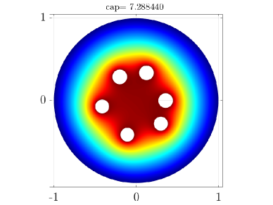
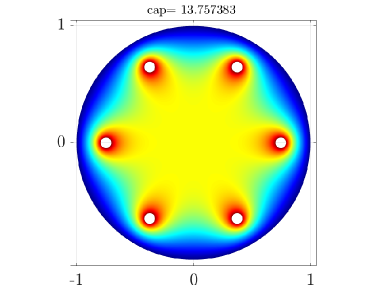
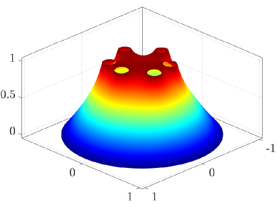
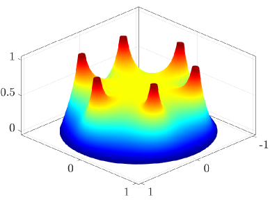
Figure 1: Surface plots of the potentials for the six hyperbolic disks with equal hyp-radii $0.2$. The centers of the disks are at the initial positions (left) and at the positions that maximize the capacity (right).

Consider a constellation $E$ of six disks with equal hyperbolic radii whose centres are contained within a subdisk, $E\subset B^{2}(0,R)$. The task is to find a configuration with maximal capacity. This is illustrated in Figure 1. Maximizing the capacity is equivalent to maximizing the $L^{2}$-norm of the gradient of the potential $u$ which is a solution of the Laplace equation where the outer boundary is set to zero and each disk to one. (For the formal definition of the capacity, see Section 2.3 below.)

Regardless of the initial configuration, the constrained maximization process moves the disks to the outer boundary and maximizes their mutual distances in terms of capacity, resulting in a symmetric configuration. This final configuration demonstrates what is referred to above as a maximal dispersion phenomenon.

1.2 Organization

The paper is organized as follows: Section 2 contains preliminary information about hyperbolic geometry, conformal capacity, and special functions to be used in the later sections. Section 3 is a description of our two computational methods, the $hp-$FEM and the boundary integral equation method. Our experimental discoveries are confirmed by these two methods. Section 4 presents our computational work on the disk constellations. Section 5 presents similar results, but now in place of the hyperbolic disks we have hyperbolic segments with fixed lengths. Section 6 draws the conclusions of our work and suggests problems for new research.

2 Preliminaries

In this section we recall some facts from hyperbolic geometry and special functions related to conformal capacity of canonical condensers.

2.1 Hyperbolic geometry

We recall some basic formulas and notation for hyperbolic geometry from [3]. The Euclidean balls with center $x\in{\mathbb{R}^{2}}$ and radius $r>0$ are denoted $B^{2}(x,r)$ and its boundary sphere is $S(x,r)$. For brevity we write ${\mathbb{B}^{2}}=B^{2}(0,1)$. The hyperbolic metric of the unit disk ${\mathbb{B}^{2}}$ is defined by

$${\rm sh}\frac{\rho_{\mathbb{B}^{2}}(a,b)}{2}=\frac{|a-b|}{\sqrt{(1-|a|^{2})(1-|b|^{2})}},\quad a,b\in\mathbb{B}^{2}.$$ (2)

The hyperbolic disk with center $x\in{\mathbb{B}^{2}}$ and radius $R>0$ is $B_{\rho}(x,R)=\{z:\rho_{\mathbb{B}^{2}}(x,z)<R\}.$ We often use the connection between the hyperbolic disk and Euclidean disk

$$\begin{cases}B_{\rho}(x,R)=B^{n}(y,r)\;,&\\ \vskip 5.0pt\cr{\displaystyle y={x(1-t^{2})\over 1-|x|^{2}t^{2}}\;,\;\;r={(1-|x|^{2})t\over 1-|x|^{2}t^{2}}\;,\;\;t={\rm th}(R/2)\;,}&\end{cases}$$ (3)

2.2 Special functions

For $|z|<1$, the Gaussian hypergeometric function is defined by the equality

$${}_{2}F_{1}(a,b;c;z)=\sum_{n=1}^{\infty}\frac{(a)_{n}(b)_{n}}{(c)_{n}}\,\frac{z^{n}}{n!},$$

$|z|<1$, where $(q)_{n}$ denotes the Pochhammer symbol, i.e. $(q)_{n}=q(q+1)\ldots(q+(n-1))$ for every natural $n$ and $(q)_{0}=1$.

The complete elliptic integral of the first kind

$${\mathcal{K}}(r)=\int_{0}^{1}\frac{dt}{\sqrt{(1-t^{2})(1-r^{2}t^{2})}}\,,\quad r\in(0,1),$$ (4)

is, in fact, a special case of the Gaussian hypergeometric function; we have

$${\mathcal{K}}(r)=\frac{\pi}{2}\,\,{}_{2}F_{1}({\textstyle\frac{1}{2}},{\textstyle\frac{1}{2}};1;r^{2}).$$

The decreasing homeomorphism $\mu:(0,1)\to(0,\infty)$

$$\mu(r)=\frac{\pi}{2}\frac{{\mathcal{K}}(\sqrt{1-r^{2}})}{{\mathcal{K}}(r)}\,,\quad 0<r<1,$$

is recurrent in the study of conformal invariants.

2.3 Condenser capacity

A condenser is a pair $(G,E)$, where $G\subset\mathbb{B}^{2}$ is a domain and $E$ is a compact non-empty subset of $G$. The conformal capacity of this condenser is defined as [7, 9, 14]

$${\rm cap}(G,E)=\inf_{u\in A}\int_{G}|\nabla u|^{2}dm,$$ (5)

where $A$ is the class of $C^{\infty}_{0}(G)$ functions $u:G\to[0,\infty)$ with $u(x)\geq 1$ for all $x\in E$ and $dm$ is the $2$-dimensional Lebesgue measure. Here we assume that $G=\mathbb{B}^{2}$ is the unit disk and $E=\cup_{j=1}^{m}E_{j}$ where $E_{1},\ldots,E_{m}$ are $m$ compact disjoint non-empty subsets of the unit disk $\mathbb{B}^{2}$ such that $\partial E_{1},\ldots,\partial E_{m}$ are smooth Jordan curves. Hence $\Omega=G\backslash E$ is a multiply connected domain of connectivity $m+1$ and the infimum in (5) is attained by a harmonic function $u$. This extremal function $u$ is the unique solution of the Laplace equation in $\Omega$ with boundary values equal $u=1$ on $E$ and $u=0$ on $\partial G$ [7]. The capacity can be then expressed in terms of the extremal function $u$ as

$${\rm cap}(G,E)=\iint\limits_{\Omega}|\nabla u|^{2}dxdy,$$ (6)

which, using Green’s formula [7, p. 4], implies that

$${\rm cap}(G,E)=\int_{\partial\Omega}u\frac{\partial u}{\partial{\bf n}}ds$$ (7)

where $\partial u/\partial{\bf n}$ denotes the directional derivative of $u$ along the outward normal. Since $u=0$ on $\partial G$ and $u=1$ on $\partial E_{k}$, we have

$${\rm cap}(G,E)=\sum_{k=1}^{m}b_{k}$$ (8)

where

$$b_{k}=\int_{\partial E_{k}}\frac{\partial u}{\partial{\bf n}}ds,\quad k=1,2,\ldots,m.$$ (9)

Thus, the constant $b_{k}$ can be considered as the contribution of the compact set $E_{k}$ to the capacity ${\rm cap}(G,E)$, for $k=1,2,\ldots,m$. Since the Dirichlet integral is conformally invariant, the cases for which $\partial E_{1},\ldots,\partial E_{m}$ are rectilinear slits can be handled with the help of auxiliary conformal mappings which transform the slits to smooth curves.

The conformal capacity of a condenser is one of the key notions of potential theory of elliptic partial differential equations [9, 15] and it has numerous applications to geometric function theory, both in the plane and in higher dimensions, [7, 9, 14, 15].

Numerous variants of the definition (5) of capacity are given in [9, 14]. For instance

$${\rm cap}(G,E)=\mathsf{M}(\Delta(E,\partial G;G)),$$ (10)

where $\Delta(E,\partial G;G)$ is the family of all curves joining $E$ with the boundary $\partial G$ in the domain $G$ and $\mathsf{M}$ stands for the modulus of a curve family [14, Ch 7]. A fundamental fact is subadditivity: if $E=\cup_{j=1}^{m}E_{j}$ where $E_{j}\subset\mathbb{B}^{n}$ for all $j,$ then

$${\rm cap}(\mathbb{B}^{n},E)\leq\sum_{j=1}^{m}{\rm cap}(\mathbb{B}^{n},E_{j}).$$ (11)

For the basic facts about capacities and moduli, the reader is referred to [7, 9, 14, 15]. The exact value of the capacity is known only in a handful of special cases. For instance, the capacity $\gamma_{2}(r)$ of the Grötzsch condenser $(\mathbb{B}^{2},[0,r])$ can be expressed as

$$\gamma_{2}(r)=2\pi/\mu(r).$$

The capacity of a spherical annulus is also known by the next lemma and (10).

Lemma 1

[14, (7.3), p. 107]
(1) If $0<a<b$ and $D=\overline{B}^{2}(0,b)\backslash B^{2}(0,a)$,

$$\mathsf{M}(\Delta(S(0,a),S(0,b);D))=2\pi/\log({b}/{a}).$$

(2) If $R>0$ then for $x\in\mathbb{B}^{2}$

$$\mathsf{M}(\Delta(S(0,1),B_{\rho}(x,R);\mathbb{B}^{2}))=2\pi/\log({1}/{{\rm th}(R/2)})\,.$$

3 Methods

In this section the numerical methods used in the numerical experiments are briefly described. The capacities of constellations are computed using the $hp$-version of the finite element method (FEM) and the boundary integral equation with the generalized Neumann kernel method (BIE). The maximization problems are computed using the interior-point method as implemented in MATLAB and Mathematica.

In any numerical study the questions of validation and verification need to be addressed. The Dirichlet problem (5) is one of the primary numerical model problems, therefore any standard solution technique can be viewed as having been validated. In the class of problems considered in this paper, verification follows through the numerical experiments below.

3.1 High-Order Finite Element Method

In constrast with the standard finite element method ($h$-version of FEM) the high-order finite element method adds a refinement parameter, the local polynomial order $p$, hence the name $p$-version. When both refinements are available we refer to $hp$-version. High-oder finite element methods have the capability for exponential convergence provided the discretisation is constructed properly in both domain (in $h$) and local polynomial order (in $p$).

In this paper in all cases it is implicitly assumed that the exact parameterisation of the boundaries on the parameter space is known. This allows us to benefit from efficient handling of large elements within the $p$-version without significant loss of accuracy, and more importantly, geometric refinements can be carried out with relative ease. This means that the number of elements can be kept relatively low.

Let us consider the Dirichlet problem (5) and its weak solution $u_{0}$. The following theorem due to Babuška and Guo [1], sets the limit to the rate of convergence of the $hp$-FEM. Notice that construction of the appropriate spaces is technical, but can be extended to parameterised surfaces. For rigorous treatment of the theory involved see Schwab [26] and references therein.

Theorem 1

Let the computational domain $G\subset\mathbb{R}^{2}$, $v$ the FEM-solution of (5), and let the weak solution $u_{0}$ be in a suitable countably normed space where the derivatives of arbitrarily high order are controlled. Then

$$\inf_{v}\|u_{0}-v\|_{H^{1}(G)}\leq C\,\exp(-b\sqrt[3]{N}),$$

where $C$ and $b$ are independent of $N$, the number of degrees of freedom. Here $v$ is computed on a proper geometric mesh, where the order of an individual element is set to be its element graph distance to the nearest singularity. (The result also holds for meshes with constant polynomial degree.)

There are many efficient error estimators available for $hp$-FEM. The so-called auxiliary subspace error estimation fits particularly well within our implementation. Let $\mathcal{T}$ be some $hp$-discretisation on the computational domain $G$. Assuming that the exact solution $u\in H_{0}^{1}(G)$, defined on $\mathcal{T}$, has finite energy, the approximation problem is as follows: Find $\hat{u}\in V$ such that

$$a(\hat{u},v)=l(v)\ (=a(u,v))\quad(\forall v\in V),$$ (12)

where $a(\,\cdot\,,\,\cdot\,)$ and $l(\,\cdot\,)$, are the bilinear form and the load potential, respectively. Additional degrees of freedom are introduced by enriching the space $V$ via introduction of an auxiliary subspace or “error space” $W\subset H_{0}^{1}(G)$ such that $V\cap W=\{0\}$. The error problem becomes thus: Find $\varepsilon\in W$ such that

$$a(\varepsilon,v)=l(v)-a(\hat{u},v)(=a(u-\hat{u},v))\quad(\forall v\in W).$$ (13)

This can be interpreted as a projection of the residual to the auxiliary space.

The main error theorem on auxiliary subspace error estimators for standard diffusion problems is given in [12]. It should be mentioned that even though there exists compelling numerical evidence that the constant $K$ is in fact independent of $p$, no rigorous proofs exist to support this observation.

3.2 A Priori Refinement Strategies

One of the implementation challenges associated with the $p$- and $hp$-version is the generation of conforming meshes with geometric grading. Often exponential convergence cannot be realised unless these special meshes have been generated.

In problems with singularities with known locations, a priori optimally refined meshes can be computed using rule based algorithms [13]. The geometric grading is illustrated in Figure 2.

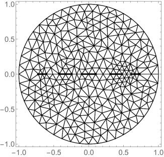
(a)

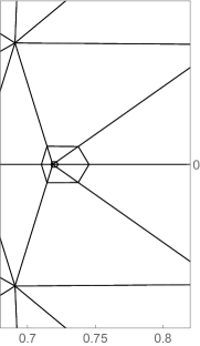
(b)

Figure 2: Mesh refinements. (A) Typical FEM mesh with the five segments on the diameter indicated with thick lines. (B) Detail of the mesh at one of the end points of the segments. Successive levels of refinements, eight altogether, are shown in the plot (the smallest ones are not visible in the given scale).

The meshing process has two steps: (a) global mesh, followed by (b) local refinements. One of the drawbacks of this approach is that almost always before one can modify the global or background mesh, the local refinements must be unwound, since typical geometric invariants of the triangulations are not valid within the local refinements, for instance, the Delaunay property (maximisation of the minimal angle). In the solution process we are content to adapt the discretisation simply by modifying the a priori strategy, in other words, by remeshing the whole domain.

3.3 BIE method

We shall consider two types of condensers $(\mathbb{B}^{2},E)$ in this paper. In the first type, the compact set $E$ is assumed to be the union of $m$ disjoint hyperbolic disks in $\mathbb{B}^{2}$. For the second type, we assumed that $E$ is the union of $m$ disjoint hyperbolic segments in $\mathbb{B}^{2}$. The capacity $\operatorname{\mathrm{cap}}(\mathbb{B}^{2},E)$, for both types of domains, can be computed using the boundary integral equation (BIE) method presented in [22]. The method is based on the BIE with the generalized Neumann kernel. This method is briefly reviewed in this section. However, before implementing the numerical method, we first convert the hyperbolic disks and segments to Euclidean ones.

3.3.1 Domains bounded by smooth curves

When $E$ is a union of $m$ disjoint hyperbolic disks, then the domain $\Omega=\mathbb{B}^{2}\backslash E$ is a bounded multiply connected domain of connectivity $m+1$ whose boundaries are circles. The orientation of the external circle $C_{0}$ is counterclockwise oriented and the inner circles $C_{1},\ldots,C_{m}$ are clockwise oriented. The external circle $C_{0}$ is parametrized by $\eta_{0}(t)$ for $t\in J_{0}=[0,2\pi]$. Each inner circle $C_{j}$ is parametrized by $\eta_{j}(t)$, $t\in J_{j}=[0,2\pi]$, for $j=1,2,\ldots,m$. Let $J$ be the disjoint union of the $m+1$ intervals $J_{j}=[0,2\pi]$, $j=0,1,\ldots,m$. We define a parametrization of the whole boundary $C=\cup_{j=0}^{m}C_{j}$ on $J$ by (see [20] for the details)

$$\eta(t)=\left\{\begin{array}[]{cc}\eta_{0}(t),&t\in J_{0},\\ \eta_{1}(t),&t\in J_{1},\\ \vdots\\ \eta_{m}(t),&t\in J_{m}.\\ \end{array}\right.$$

With the parametrization $\eta(t)$ of the whole boundary $C$, we define a complex function $A$ by

$$A(t)=\eta(t)-\alpha,$$ (14)

where $\alpha$ is a given point in the domain $\Omega$. For each $k=1,2,\ldots,m$, let $z_{k}$ be a given point interior to the circle $C_{k}$, let the function $\gamma_{k}$ be defined by

$$\gamma_{k}(t)=\log|\eta(t)-z_{k}|,$$ (15)

and let $\mu_{k}$ be the unique solution of the BIE

$$\mu_{k}-{\bf N}\mu_{k}=-{\bf M}\gamma_{k},$$ (16)

where ${\bf N}$ is the integral operator with the generalized Neumann kernel

$$N(s,t):=\frac{1}{\pi}\operatorname{\mathrm{Im}}\left(\frac{A(s)}{A(t)}\frac{\eta^{\prime}(t)}{\eta(t)-\eta(s)}\right),\quad(s,t)\in J\times J,$$ (17)

and ${\bf M}$ is the integral operator with the kernel

$$M(s,t):=\frac{1}{\pi}\operatorname{\mathrm{Re}}\left(\frac{A(s)}{A(t)}\frac{\eta^{\prime}(t)}{\eta(t)-\eta(s)}\right),\quad(s,t)\in J\times J.$$ (18)

Then the function $h_{k}$ given by

$$h_{k}=[{\bf M}\mu_{k}-({\bf I}-{\bf N})\gamma_{k}]/2$$ (19)

is a piecewise constant function, i.e.,

$$h_{k}(t)=\left\{\begin{array}[]{cc}h_{0,k},&t\in J_{0},\\ h_{1,k},&t\in J_{1},\\ \vdots\\ h_{m,k},&t\in J_{m},\\ \end{array}\right.$$

where $h_{0,k},h_{1,k},\ldots,h_{m,k}$, $k=1,2,\ldots,m$, are real constants. The capacity $\operatorname{\mathrm{cap}}(\mathbb{B}^{2},E)$ can be then computed by [22, Eq. (3.9)]

$$\operatorname{\mathrm{cap}}(\mathbb{B}^{2},E)=2\pi\sum_{k=1}^{m}a_{k},$$ (20)

where the values of the $m$ real constants $a_{1},\ldots,a_{m}$ are computed by solving the $(m+1)\times(m+1)$ linear system

$$\left[\begin{array}[]{ccccc}h_{0,1}&h_{0,2}&\cdots&h_{0,m}&1\\ h_{1,1}&h_{1,2}&\cdots&h_{1,m}&1\\ \vdots&\vdots&\ddots&\vdots&\vdots\\ h_{m,1}&h_{m,2}&\cdots&h_{m,m}&1\\ \end{array}\right]\left[\begin{array}[]{c}a_{1}\\ a_{2}\\ \vdots\\ a_{m}\\ c\end{array}\right]=\left[\begin{array}[]{c}0\\ 1\\ \vdots\\ 1\end{array}\right].$$ (21)

The constants $b_{1},\ldots,b_{m}$ in (9) are related to the constants $a_{1},\ldots,a_{m}$ by

$$b_{k}=2\pi a_{k},\quad k=1,2,\ldots,m.$$ (22)

The BIE (16) can be discretized by the Nyström method with the trapezoidal rule to obtain an $(m+1)n\times(m+1)n$ linear system where $n$ is the number of the discretization points in each boundary component. The linear system can then be solved by the MATLAB function gmres and the matrix-vector product in gmres can be computed in $O(mn)$ operations using the MATLAB function zfmm2dpart from the fast multipole method (FMM) MATLAB toolbox FMMLIB2D [10]. This method for solving the BIE (16) was implemented in the MATLAB function fbie presented in [20]. The MATLAB function fbie provides us with approximations to the solution $\mu_{k}$ of the BIE (16) as well as the piecewise constant function $h_{k}$ in (19). The computed values of $h_{k}$ are used to set up the $(m+1)\times(m+1)$ linear system (21), which will be solved using the Gauss elimination method (here $m+1$ is the number of boundary components of the domain $G$ which is usually small). By computing the constants $a_{1},\ldots,a_{m}$, the value of the capacity $\operatorname{\mathrm{cap}}(G,E)$ is given by (20). Further, the values of the constants $b_{1},\ldots,b_{m}$ are given by (22). See [20, 22] for details.

3.3.2 Domains bounded by slits

The BIE method presented above can be used to compute the capacity of only condensers bounded by smooth or piecewise Jordan curves [20, 22]. Since the Dirichlet integral is conformally invariant, the capacities for the cases for which the plates of the condenser are slits can be computed with the help of conformal mappings. In this paper, we consider two types of domains $G$ bounded by slits.

In the first case, we assume that $\Omega$ is the unit disk with $m$ radial slits. For such a case, we can use the iterative method presented in [21] to compute a conformally equivalent domain $D$ bounded by smooth Jordan curves so that our method presented in Section 3.3.1 can be used. An example of the domain $\Omega$ and its conformally equivalent computed domain $D$ for $m=6$ is presented in Figure 3.

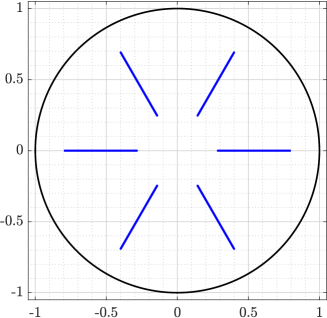
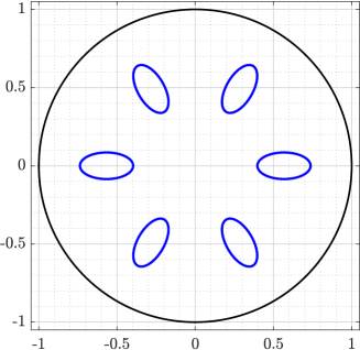
Figure 3: An example of the given unit disk with radial slit domain $\Omega$ (left) and its conformally equivalent computed domain $D$ (right).

In the second case, we assume that $\Omega$ is the unit disk with $m$ rectilinear slits on the real line (see Figure 4 (left) for $m=5$). Unlike the domain in the first case, this domain is not one of the canonical slit domains (see [17, 19]). Thus, in this case, we first consider the unbounded domain $\hat{\Omega}$ in the exterior of the $m$ rectilinear slits which is a canonical slit domain (see Figure 5 (left) for $m=5$). We use the iterative method presented in [21] to compute a conformally equivalent domain $\hat{D}$ in the exterior of $m$ smooth Jordan curves and the conformal mapping $w=\Phi(z)$ from the domain $\hat{D}$ onto $\hat{\Omega}$ (see Figure 5 (right) for $m=5$). Hence, $z=\Phi^{-1}(w)$ is a conformal mapping from the domain $\hat{\Omega}$ onto $\hat{D}$. Since the unit circle is in the interior of the domain $\hat{\Omega}$, the conformal mapping $z=\Phi^{-1}(w)$ can be used to compute the image of the unit circle which will be a smooth Jordan curve exterior to the computed $m$ smooth Jordan curves. Thus, the conformal mapping $z=\Phi^{-1}(w)$ maps the given domain $\Omega$ onto a conformally equivalent domain $D$ bounded by smooth Jordan curves so that the method reviewed in Section 3.3.1 can be used (see Figure 4 (right) for $m=5$). Notice that the external curve in Figure 4 (right) is not a circle.

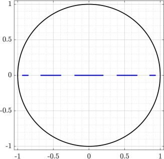
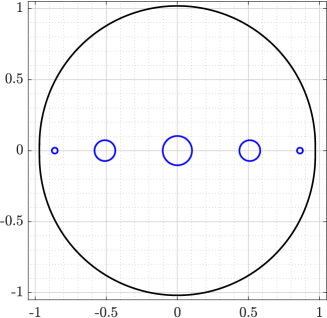
Figure 4: An example of the given unit disk with rectilinear slit domain $\Omega$ (left) and the conformally equivalent computed domain $D$ (right).

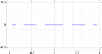
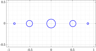
Figure 5: An example of the rectilinear slit domain $\hat{\Omega}$ (left) and the conformally equivalent computed domain $\hat{D}$ (right).

For details on the iterative method for computing the domain $D$ for both cases of slit domains discussed above, we refer the reader to [21] (see also [16] for other types of slit domains).

3.4 Nonlinear Optimization: Interior-Point Method

The numerical optimization algorithm of our choice is the interior-point method as implemented in Mathematica (FindMaximum, [28]) and Matlab (fmaxcon, [18]). The task is to find an optimal configuration for a constellation of hyperbolic disks $E$ with fixed radii, where at every step the current configuration if solved using either one of the methods described above. The standard textbook reference is Nocedal and Wright [24].

In the most general case the problem is defined as in (23), where the only constraints are geometric ones, that is, the disks are not allowed to overlap, and they are not allowed to drift to the boundary, for instance, they must lie within a disk $\mathbb{D}_{R}$ with same prescribed radius $R$, or alternatively their centers must lie inside some constraining disk. The radii are fixed and the optimization concerns only the locations of the disks.

The maximization problem is formally defined as

$$\max_{E} {\rm cap}(G,E)$$

subject to: $$E_{i}\cap E_{j} =\emptyset \quad\forall\ i,j=1,\ldots,m,i\neq j$$ (23)

$$E_{j} \subset\mathbb{D}_{R} \quad\forall\ j=1,\ldots,m.$$

This nonlinear optimization problem can be solved using the interior-point method, and the solution would be a local maximum.

Notice, that the objective function is indeed the capacity of the constellation. The number of evaluations is greater than the number of iteration steps, since the gradients and Hessians must be approximated numerically. One of the insights gained over many such computations is that the optimization depends on the high accuracy of the capacity solver, since otherwise the approximate derivatives are not sufficiently accurate.

In the context of this work, there have been no attempts to devise a special method that would incorporate some of the insights gathered during this study. Instead, the numerical optimization is used to challenge those insights and therefore the optimizations have been computed with minimal input information.

4 Numerical experiments: Constellations of circular domains

In this section the focus is on constellations of disks. In the maximisation of the capacity the positions of the disks are subject to two types of geometric constraints, they are either constrained to a disk of given radius or an interval of fixed length on the real line. The experiments in turn either cover full parameter ranges or are general in the sense that the initial configurations are random, but satisfy the constraints, of course. We first consider constellations of two disks of equal hyperbolic radii, and then extend the investigation to constellations with six disks constrained to a disk, and to constellations with five disks with centers constrained to an interval. In the two latter cases also the case of unequal hyperbolic radii is studied. In the final experiment the constellation is condensed into a single disk with equal capacity. The objective is to compare the hyperbolic area and perimeter of a constellation to that of a condensed one.

4.1 Constellation of two disks with constrained positions

We begin with the constellation $E$, union of two hyperbolic disks $D_{1}$ and $D_{2}$ with equal hyp-radius $r$. First we assume that the centers of these disks are on $Re^{\pm\mathrm{i}\theta}$ where $0<\theta_{\rm min}<\theta<\pi-\theta_{\rm min}<\pi$ and

$$\theta_{\rm min}=\arcsin\left(\frac{(1-R^{2})\operatorname{\mathrm{sh}}r}{2R}\right).$$

See Figure 6 (left) for $R=0.5$ and $\theta=\pi/4$. The two disks touch each other when $\theta=\theta_{\rm min}$ or $\theta=\pi-\theta_{\rm min}$. When $r=0.1$, the values of $\operatorname{\mathrm{cap}}({\mathbb{D}},E)$ vs. $\theta$ are shown in Figure 7 (left) for several values of $R$.

Then we assume that the centers of these disks are on $\pm x$ where $x_{\rm min}<x<1$ and $x_{\rm min}=\,\textnormal{th}(r/2)$ where the two disks touch each other when $x=x_{\rm min}$ (See Figure 6 (right) for $x=0.5$). The values of $\operatorname{\mathrm{cap}}({\mathbb{D}},E)$ for $r=0.1$ vs. $x$ are shown in Figure 7 (right).

Note that $\operatorname{\mathrm{cap}}({\mathbb{D}},D_{i})=-2\pi/\log(\,\textnormal{th}(r/2))$, $i=1,2$. For $r=0.1$, the values of $\operatorname{\mathrm{cap}}({\mathbb{D}},D_{1})$ are shown in Figure 7 as “dashed line” and the values of $\operatorname{\mathrm{cap}}({\mathbb{D}},D_{1})+\operatorname{\mathrm{cap}}({\mathbb{D}},D_{2})$ as “dotted line.”

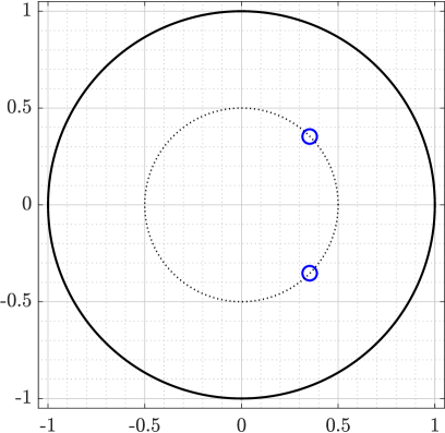
(a)

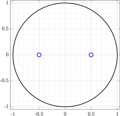
(b)

Figure 6: Two hyperbolic disks with hyp-radius $0.1$. The centers of the two disks are $Re^{\pm\mathrm{i}\theta}$ for $R=0.5$ and $\theta=\pi/4$ (left) and $\pm x$ for $x=0.5$ (right).

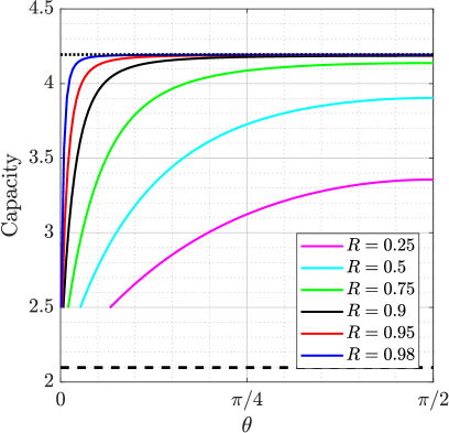
(a)

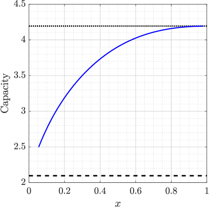
(b)

Figure 7: The capacity for two hyperbolic disks with hyp-radius $r=0.1$ . The centers of the two disks are $Re^{\pm\mathrm{i}\theta}$ (left) and $\pm x$ (right), where the leftmost point on the curve corresponds to Cartesian coordinate $\,\textnormal{th}(r/2)\approx 0.05$, that is, when the two disks touch.

4.2 Constellation of six disks constrained to a disk

We increase the number of disks and consider the positions of a constellation of six hyperbolic disks that maximize the capacity $\operatorname{\mathrm{cap}}({\mathbb{D}},E)$ under the constraint that the hyperbolic centers of these disks are inside the Euclidean disk $|z|\leq R$ (we assume in the examples below that $R=0.75$). The disks are numbered $D_{1}$ to $D_{6}$ in counterclockwise orientation. We denote the center of the disk $D_{j}$ by $z_{j}$, $j=1,\ldots,6$. Without any loss of generality, we assume that the center $z_{1}$ of the disk $D_{1}$ lies on the positive real axis.

First we assume that all six disks have equal hyperbolic radii $=0.2$, and the initial positions are random within the given constraints. The configuration which maximizes the capacity $\operatorname{\mathrm{cap}}({\mathbb{D}},E)$ has the maximal dispersion property: The positions of these six disks are on the Euclidean circle $|z|=R$ and, moreover, are symmetric, that is, the hyperbolic distances between the centers of any two adjacent disks are equal (see Figure 8(A) and Table 1). The computed capacity $=13.757381$.

When the hyperbolic radius of one of these disks is changed either to $0.4$ (see Figure 8(B)) or $0.8$ (see Figure 8(C)), the centers of the other disks move away from the larger disk (see Table 1), yet rotational symmetry is preserved for the maximal configuration. To study closely the impact of increasing the hyperbolic radius of only one disk on the positions that maximize the capacity $\operatorname{\mathrm{cap}}({\mathbb{D}},E)$, we assume that the hyperbolic radius of the first disk $D_{1}$ is $r_{1}$ and the hyperbolic radii of the remaining five disks $D_{2}$–$D_{6}$ are $0.2$. As above, we find the positions of these six disks that maximize the capacity $\operatorname{\mathrm{cap}}({\mathbb{D}},E)$ under the above constraint. For the positions that maximizes the capacity $\operatorname{\mathrm{cap}}({\mathbb{D}},E)$, we compute the hyperbolic distances $\rho(z_{1},z_{2})$, $\rho(z_{2},z_{3})$, and $\rho(z_{3},z_{4})$ and the values of the constants $b_{1}$, $b_{2}$, $b_{3}$, and $b_{4}$ in (22) where the values of $r_{1}$ are changing from $0.2$ to $2$. The obtained numerical results are presented in Figure 9. Notice that the constant $b_{k}$ can be regarded as the contribution of the disk set $D_{k}$ to the capacity ${\rm cap}(G,E)$, for $k=1,2,\ldots,m$. As we can see, the values of $b_{1}$ increased as $r_{1}$ increased and the values of $b_{2}$, $b_{3}$, and $b_{4}$ are almost constants. Notice also that, due to symmetry, $\rho(z_{1},z_{2})=\rho(z_{1},z_{6})$, $\rho(z_{2},z_{3})=\rho(z_{6},z_{5})$, $\rho(z_{3},z_{4})=\rho(z_{5},z_{4})$, $b_{5}=b_{3}$, and $b_{6}=b_{2}$.

If the hyperbolic radii of two of these six disks are changed to either $0.4$ or $0.8$, the natural symmetries induce three local maxima as shown in Figure 11. The hyperbolic distances between the centers of any two adjacent disks for all cases in Figure 11 are shown in Table 2. Similarly, with three disks three local maxima are observed (see Figure 12 and Table 3).

Considering the results for constellations of disks with unequal radii we can observe that in all cases the maximal dispersion property is again observed: In the configuration which maximizes the capacity $\operatorname{\mathrm{cap}}({\mathbb{D}},E)$ the positions of these six disks are on the Euclidean circle $|z|=R$.

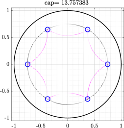
(a)

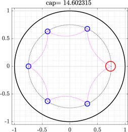
(b)

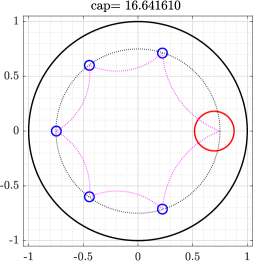
(c)

Figure 8: Disk 1 has hyp-radius $0.2$ (left), $0.4$ (center), and $0.8$ (right). Disks 2 through 6 have hyp-radii 0.2.

Table 1: The hyperbolic distances between the centers of consecutive disks in Figure 8.

Case	Capacity	$\rho(z_{1},z_{2})$	$\rho(z_{2},z_{3})$	$\rho(z_{3},z_{4})$	$\rho(z_{4},z_{5})$	$\rho(z_{5},z_{6})$	$\rho(z_{6},z_{1})$
A	$13.7574$	$2.6161$	$2.6161$	$2.6161$	$2.6161$	$2.6161$	$2.6161$
B	$14.6023$	$2.7393$	$2.5532$	$2.5482$	$2.5482$	$2.5532$	$2.7393$
C	$16.6416$	$2.9128$	$2.4504$	$2.4363$	$2.4363$	$2.4504$	$2.9128$

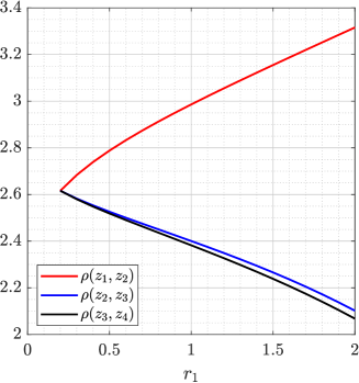
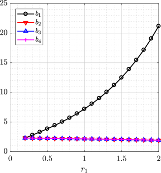
Figure 9: The hyperbolic distances between the centers of consecutive disks (left) and the values of the constants $b_{1}$, $b_{2}$, $b_{3}$, and $b_{4}$ in (9) (right) as functions of $r_{1}$.

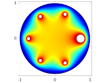
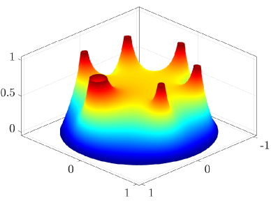
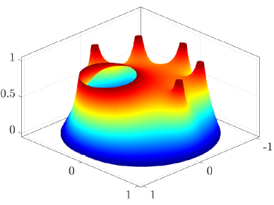
Figure 10: Surface plots of the potentials for the six hyperbolic disks where the Disk 1 has hyp-radius $r_{1}$ and Disks 2 through 6 have hyp-radii $0.2$ for $r_{1}=0.5$ (left) and $r_{1}=1.5$ (right). The centers are at the positions that maximize the capacity.

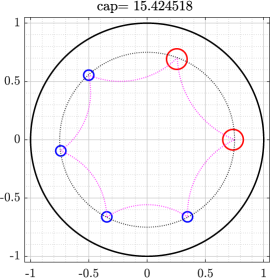
(a)

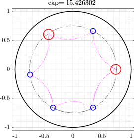
(b)

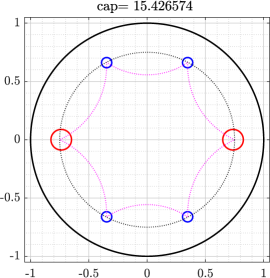
(c)

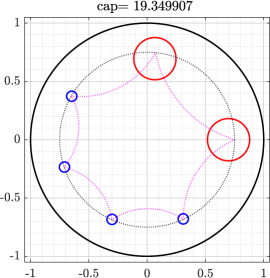
(d)

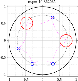
(e)

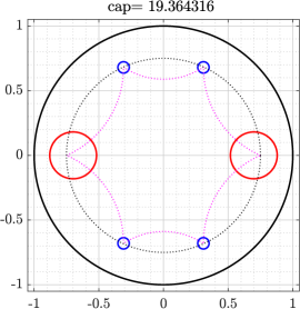
(f)

Figure 11: First row: Four disks with hyp-radii 0.2 and two disks with hyp-radii 0.4. Second row: Four disks with hyp-radii 0.2 and two disks with hyp-radii 0.8.

Table 2: The hyperbolic distances between the centers of consecutive disks in Figure 11.

Case	Capacity	$\rho(z_{1},z_{2})$	$\rho(z_{2},z_{3})$	$\rho(z_{3},z_{4})$	$\rho(z_{4},z_{5})$	$\rho(z_{5},z_{6})$	$\rho(z_{6},z_{1})$
A	$15.4245$	$2.8523$	$2.6767$	$2.4861$	$2.4815$	$2.4861$	$2.6767$
B	$15.4263$	$2.6800$	$2.6800$	$2.6742$	$2.4867$	$2.4867$	$2.6742$
C	$15.4266$	$2.6747$	$2.4920$	$2.6747$	$2.6747$	$2.4920$	$2.6747$
D	$19.3499$	$3.1452$	$2.7534$	$2.2784$	$2.2672$	$2.2784$	$2.7534$
E	$19.3620$	$2.7700$	$2.7700$	$2.7519$	$2.2813$	$2.2813$	$2.7519$
F	$19.3643$	$2.7553$	$2.2965$	$2.7553$	$2.7553$	$2.2965$	$2.7553$

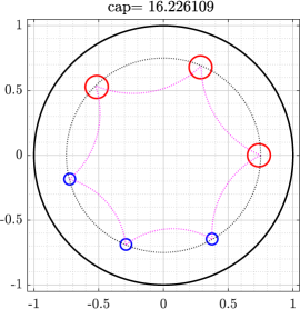
(a)

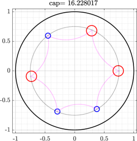
(b)

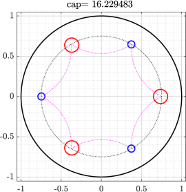
(c)

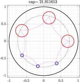
(d)

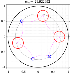
(e)

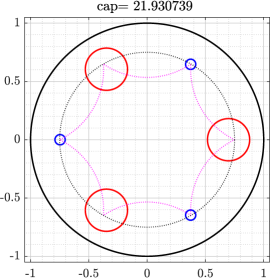
(f)

Figure 12: First row: Three disks with hyp-radii 0.2 and three disks with hyp-radii 0.4. Second row: Three disks with hyp-radii 0.2 and three disks with hyp-radii 0.8.

Table 3: The hyperbolic distances between the centers of consecutive disks in Figure 12.

Case	Capacity	$\rho(z_{1},z_{2})$	$\rho(z_{2},z_{3})$	$\rho(z_{3},z_{4})$	$\rho(z_{4},z_{5})$	$\rho(z_{5},z_{6})$	$\rho(z_{6},z_{1})$
A	$16.2261$	$2.7931$	$2.7931$	$2.6126$	$2.4210$	$2.4210$	$2.6126$
B	$16.2280$	$2.7903$	$2.6189$	$2.6161$	$2.6108$	$2.4263$	$2.6135$
C	$16.2295$	$2.6161$	$2.6161$	$2.6161$	$2.6161$	$2.6161$	$2.6161$
D	$21.9116$	$3.0047$	$3.0047$	$2.6025$	$2.1205$	$2.1205$	$2.6025$
E	$21.9225$	$3.0015$	$2.6190$	$2.6172$	$2.6035$	$2.1336$	$2.6053$
F	$21.9307$	$2.6161$	$2.6161$	$2.6161$	$2.6161$	$2.6161$	$2.6161$

4.3 Constellation of five disks constrained to the real line

Next we consider a constellation of five hyperbolic disks under the constraint that the hyperbolic centers of these disks lie within the interval $[-R,R]$. The disks are numbered ($D_{1}$-$D_{5}$) from left to right, and $R=0.75$ in all experiments.

The set of experiments follows that of the previous section. Four cases are considered: (a) all five disks have equal hyperbolic radii $=0.2$, (b) one of the disks has radius $=0.4$, (c) two disks have radius $=0.4$, and finally (d) three disks have radius $=0.4$.

All configurations up to symmetry are summarized in Figures 13,  14,  15, and Tables 4,  5,  6, for (a) and (b), (c), and (d), respectively. The maximal configurations exhibit the maximal dispersion property on a diameter: $D_{1}$ and $D_{5}$ lie at the end points of the interval, $D_{1}$ and $D_{5}$ have the largest radii, and if there are two or more disks with equal and largest radius, then the distances between the disks are symmetric about the origin.

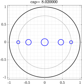
(a)

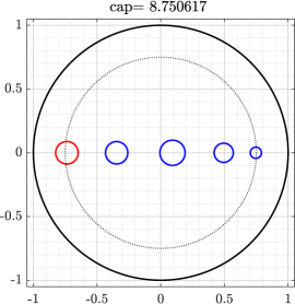
(b)

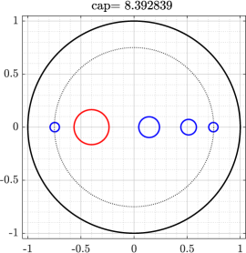
(c)

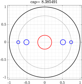
(d)

Figure 13: First row: All disks have hyp-radius $0.2$. Second row: One disk with hyp-radius $0.4$ (red) and four disks with hyp-radii 0.2 (blue).

Table 4: The hyperbolic distances between the centers of consecutive disks in Figure 13.

Case	Capacity	$\rho(z_{1},z_{2})$	$\rho(z_{2},z_{3})$	$\rho(z_{3},z_{4})$	$\rho(z_{4},z_{5})$
A	$8.0200$	$0.9467$	$0.9992$	$0.99920$	$0.9467$
B	$8.7506$	$1.2166$	$0.9160$	$0.90604$	$0.8532$
C	$8.3928$	$1.0656$	$1.1689$	$0.85703$	$0.8003$
D	$8.3855$	$0.7943$	$1.1516$	$1.1516$	$0.7943$

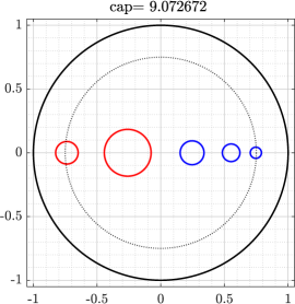
(a)

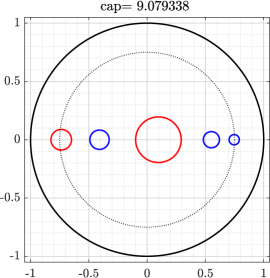
(b)

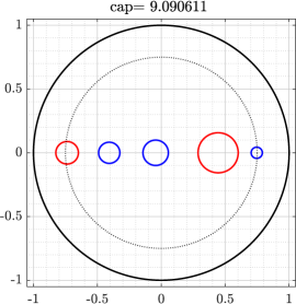
(c)

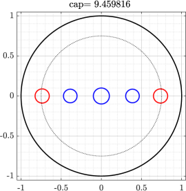
(d)

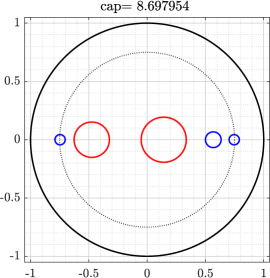
(e)

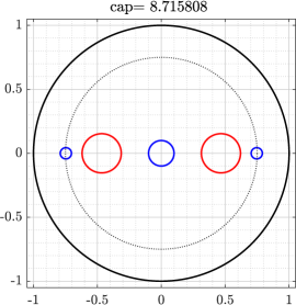
(f)

Figure 14: Two disks have hyp-radius $0.4$ (red) and three disks have hyp-radii 0.2 (blue).

Table 5: The hyperbolic distances between the centers of consecutive disks in Figure 14.

Case	Capacity	$\rho(z_{1},z_{2})$	$\rho(z_{2},z_{3})$	$\rho(z_{3},z_{4})$	$\rho(z_{4},z_{5})$
A	$9.0727$	$1.3935$	$1.0596$	$0.7477$	$0.6910$
B	$9.0793$	$1.0701$	$1.0777$	$1.0488$	$0.6953$
C	$9.0906$	$1.0733$	$0.7834$	$1.0806$	$0.9545$
D	$9.4598$	$1.1210$	$0.8249$	$0.8249$	$1.1210$
E	$8.6980$	$0.8745$	$1.3693$	$1.0007$	$0.6473$
F	$8.7158$	$0.8971$	$1.0488$	$1.0488$	$0.8971$

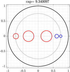
(a)

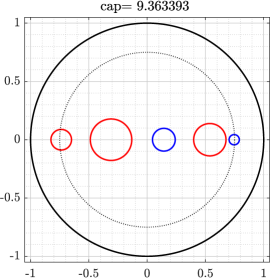
(b)

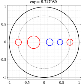
(c)

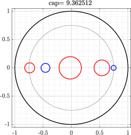
(d)

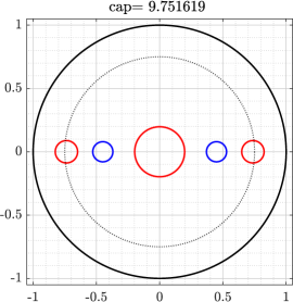
(e)

Figure 15: Three disks have hyp-radius $0.4$ (red) and two disks have hyp-radii 0.2 (blue).

Table 6: The hyperbolic distances between the centers of consecutive disks in Figure 15.

Case	Capacity	$\rho(z_{1},z_{2})$	$\rho(z_{2},z_{3})$	$\rho(z_{3},z_{4})$	$\rho(z_{4},z_{5})$
A	$9.3401$	$1.2558$	$1.2719$	$0.7477$	$0.5005$
B	$9.3634$	$1.2810$	$0.9565$	$0.9534$	$0.7010$
C	$9.7471$	$1.3014$	$0.9656$	$0.6684$	$0.9564$
D	$9.3625$	$0.9473$	$0.9550$	$1.2930$	$0.6966$
E	$9.7516$	$0.9693$	$0.9766$	$0.9766$	$0.9693$

4.4 Condensation of a constellation of $m$ disks into one disk

We study now the condensation of a constellation $E$ of $m$ hyperbolic disks with equal radii $r$ into the case of one hyperbolic disk constellation with equal capacity, and compare the hyperbolic area and perimeter of the original and the new constellation. That is, we assume that $E=\cup_{j=1}^{m}B_{\rho}(z_{j},r)$ and we will find the value of $R$ such that $\operatorname{\mathrm{cap}}(\mathbb{B}^{2},E)=\operatorname{\mathrm{cap}}(\mathbb{B}^{2},B_{\rho}(0,R))$. Recall first that the hyperbolic area and hyperbolic perimeter of a hyperbolic disk $B_{\rho}(z_{j},r)$ are by [3, Thm 7.2.2, p. 132]

$$4\pi\operatorname{\mathrm{sh}}^{2}\left(\frac{r}{2}\right)\quad{\rm and}\quad 2\pi\operatorname{\mathrm{sh}}r,$$ (24)

respectively.

Let $c=\operatorname{\mathrm{cap}}({\mathbb{D}},E)$, which will be approximated numerically using the above discussed BIE method. Since, by (1),

$$\operatorname{\mathrm{cap}}(\mathbb{B}^{2},B_{\rho}(0,R))=2\pi/\log(1/\,\textnormal{th}(R/2))\,,$$ (25)

the value of the radius $R$ of a single disk $B_{\rho}(0,R)$ with capacity equal to $c$ satisfies

$$2\,\pi/\log(1/{\rm th}(R/2))=c$$

and hence

$$R=2\,\textnormal{arth}(e^{-2\pi/c})=-\log\,\textnormal{th}(\pi/c).$$ (26)

As an example, we assume that $m=6$ and the centers $z_{j}$ of the hyperbolic disks $B_{\rho}(z_{j},r)$ are given by

$$z_{j}=0.75e^{2\pi(j-1)\mathrm{i}/m},\quad j=1,2,\ldots,m.$$

We compute the capacity $c=\operatorname{\mathrm{cap}}({\mathbb{D}},E)$ using the above BIE method with $n=2^{10}$. Then, we compute the values of $R$ via (26). The computed values of $R$ for $0.1\leq r\leq 1.2$ are presented in Figure 16. Then, by (24), the hyperbolic area and perimeter of the disk $B_{\rho}(0,R)$ are equal to $4\pi\operatorname{\mathrm{sh}}^{2}\left(\frac{R}{2}\right)$ and $2\pi\operatorname{\mathrm{sh}}R$, respectively. Note that the hyperbolic area and perimeter of $E$ are given by

$$4m\pi\operatorname{\mathrm{sh}}^{2}\left(\frac{r}{2}\right)\quad{\rm and}\quad 2m\pi\operatorname{\mathrm{sh}}r,$$

respectively. The hyperbolic area and perimeter of $E$ and $B_{\rho}(0,R)$ are presented in Figure 16. The obtained results show that the hyperbolic area of the single disk $B_{\rho}(0,R)$ is always greater than the sum of the hyperbolic area of the six disks. However, the hyperbolic perimeter of the single disk $B_{\rho}(0,R)$ is greater than the sum of the hyperbolic perimeter of the six disks for small values of $r$. For large values of $r$, the perimeter of the six disks is greater than the perimeter of the single disk.

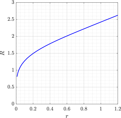
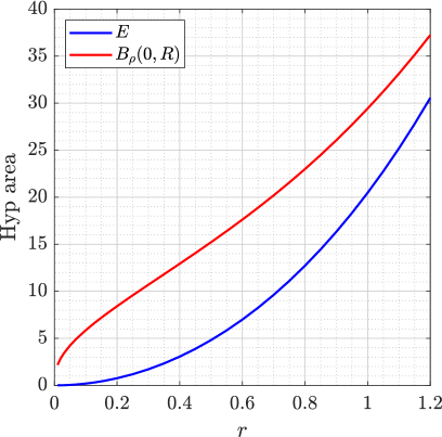
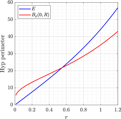
Figure 16: The values of $R$, the hyperbolic area, and the hyperbolic perimeter vs. $r$.

5 Numerical Experiments: slit constellations

In this section the elements of the constellations are hyperbolic segments of constant length. The experiments follow the same pattern as those above, however, the constraints on configurations are more restrictive. Again, we start with two segments and then increase complexity by adding more segments to the constellations.

5.1 Constellation of two hyperbolic segments

We assume that the constellation $E$ is the union of two non-overlapping hyperbolic symmetric collinear segments $I_{1}$ an $I_{2}$ with equal hyp-length $\ell$ such that the centers of these segments are $\pm xe^{\mathrm{i}\theta}$ on the line $\arg(z)=\theta\in[0,\pi)$ where

$$\,\textnormal{th}\frac{\ell}{4}<x<1,$$

and hence $\rho\left(-xe^{\mathrm{i}\theta},xe^{\mathrm{i}\theta}\right)>\ell$. The values of $\operatorname{\mathrm{cap}}({\mathbb{D}},E)$ vs. $x$ are shown in Figure 17(left) for $\theta=0$, $\ell=1$ and in Figure 17 (right) for $\theta=0$, $\ell=2$. Note that

$$\operatorname{\mathrm{cap}}({\mathbb{D}},I_{i})=\frac{2\pi}{\mu(\,\textnormal{th}(\ell/2))},\quad i=1,2,$$

and hence

$$\operatorname{\mathrm{cap}}({\mathbb{D}},I_{1})+\operatorname{\mathrm{cap}}({\mathbb{D}},I_{2})=2\operatorname{\mathrm{cap}}({\mathbb{D}},I_{1})=\frac{4\pi}{\mu(\,\textnormal{th}(\ell/2))}$$

is an upper bound for $\operatorname{\mathrm{cap}}({\mathbb{D}},E)$. The values of this upper bound are shown in Figure 17 as “dotted line.”

The two segments merge into one segment $\hat{I}$ of hyperbolic length $2\ell$ when $x=\,\textnormal{th}\frac{\ell}{4}$. Thus

$$\operatorname{\mathrm{cap}}({\mathbb{D}},\hat{I})=\frac{2\pi}{\mu(\,\textnormal{th}(\ell))}$$

is a lower bound for for $\operatorname{\mathrm{cap}}({\mathbb{D}},E)$. The values of $\operatorname{\mathrm{cap}}({\mathbb{D}},\hat{I})$ are shown in Figure 17 as “dashed line.”

Figure 17 shows that $\operatorname{\mathrm{cap}}({\mathbb{D}},E)\to 4\pi/\mu(\,\textnormal{th}(\ell/2))$ as $x\to 1$ and $\operatorname{\mathrm{cap}}({\mathbb{D}},E)\to 2\pi/\mu(\,\textnormal{th}(\ell))$ as $x\to\,\textnormal{th}(\ell/4)$.

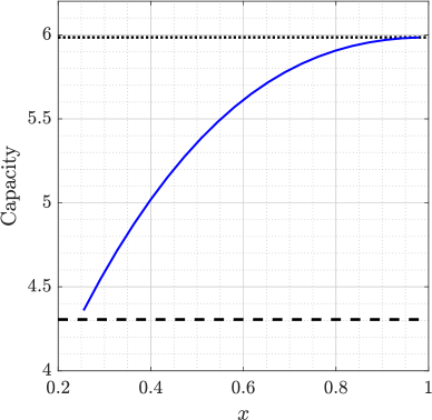
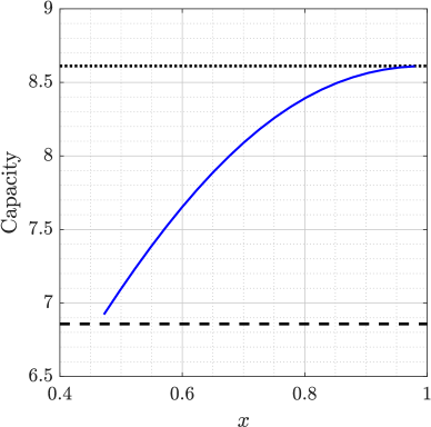
Figure 17: Two hyperbolic segments with hyp-length $\ell=1$ (left) $\ell=2$ (right). The centers of these segments are $\pm xe^{\mathrm{i}\theta}$ for $\theta=0$.

5.2 Constellation of five radial hyperbolic segments with constant angle of separation

Next we let $E$ be the union of five non-overlapping hyperbolic segments, $I_{1},\ldots,I_{5}$, with equal hyp-length $\ell$ such that the center of the segment $I_{k}$ is $xe^{2k\pi\mathrm{i}/5}$ where

$$\,\textnormal{th}\frac{\ell}{4}<x<1.$$

The computed approximate values of $\operatorname{\mathrm{cap}}({\mathbb{D}},E)$ vs. $x$ are shown in Figure 18 (left) for $\ell=1$ and in Figure 18 (right) for $\ell=2$. Note that the five segments merge into one connected set $\hat{I}$ when $x=\,\textnormal{th}\frac{\ell}{4}$. Thus, using the same approach used in [23, Lemma 6.8], we can prove that

$$\operatorname{\mathrm{cap}}({\mathbb{D}},\hat{I})=\frac{10\pi}{\mu(\,\textnormal{th}^{5}(\ell/2))}$$

which is a lower bound for $\operatorname{\mathrm{cap}}({\mathbb{D}},E)$. The values of $\operatorname{\mathrm{cap}}({\mathbb{D}},\hat{I})$ are shown in Figure 18 as “dashed line.” As in the previous example,

$$\sum_{k=1}^{5}\operatorname{\mathrm{cap}}({\mathbb{D}},I_{k})=5\operatorname{\mathrm{cap}}({\mathbb{D}},I_{1})=\frac{10\pi}{\mu(\,\textnormal{th}(\ell/2))}$$

is an upper bound for $\operatorname{\mathrm{cap}}({\mathbb{D}},E)$. The values of this upper bound are shown in Figure 18 as “dotted line.”

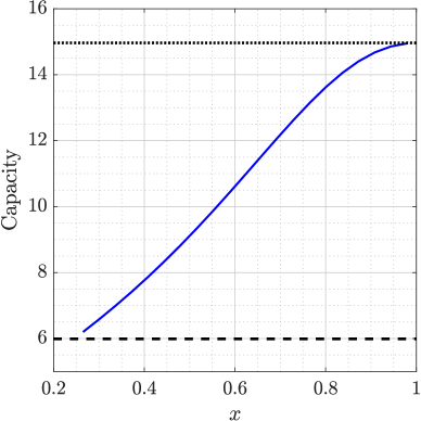
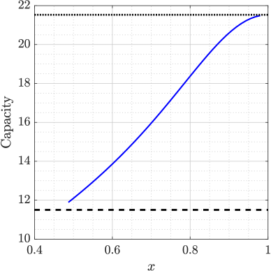
Figure 18: Five radial hyperbolic segments with hyp-length $\ell=1$ (left) $\ell=2$ (right). The centers of these segments are $xe^{2k\pi\mathrm{i}/5}$, $k=1,\ldots,5$.

For numerical computing of the capacity $\operatorname{\mathrm{cap}}({\mathbb{D}},\hat{I})$, we use the $hp$-FEM where the absolute error in the computed capacity are $2\times 10^{-12}$ and $8\times 10^{-12}$ for the short and long segments, respectively. Plots of the potential function for the capacity $\operatorname{\mathrm{cap}}({\mathbb{D}},E)$ are presented in Figure 19.

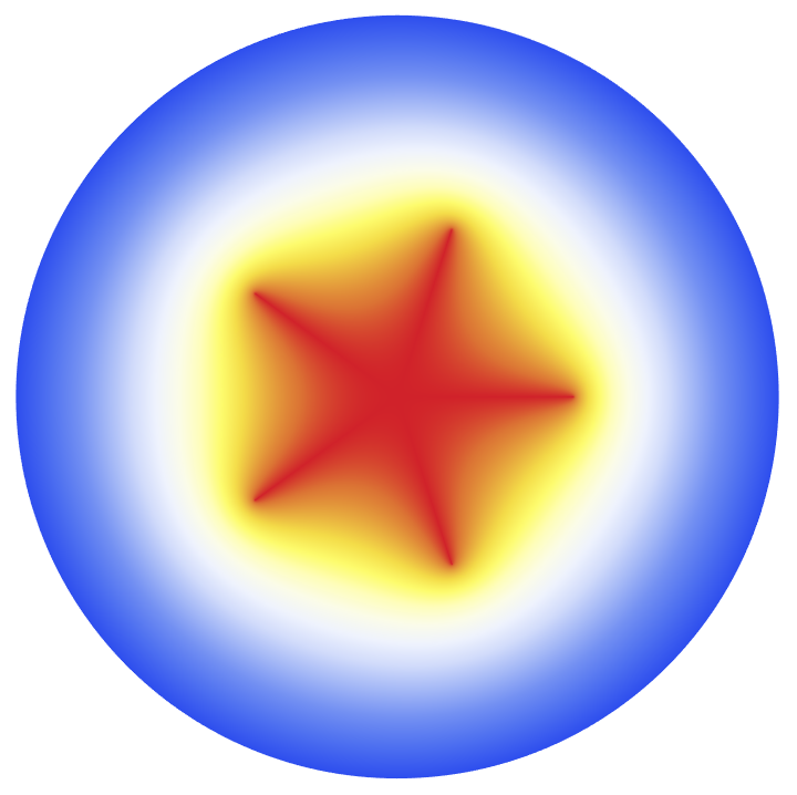
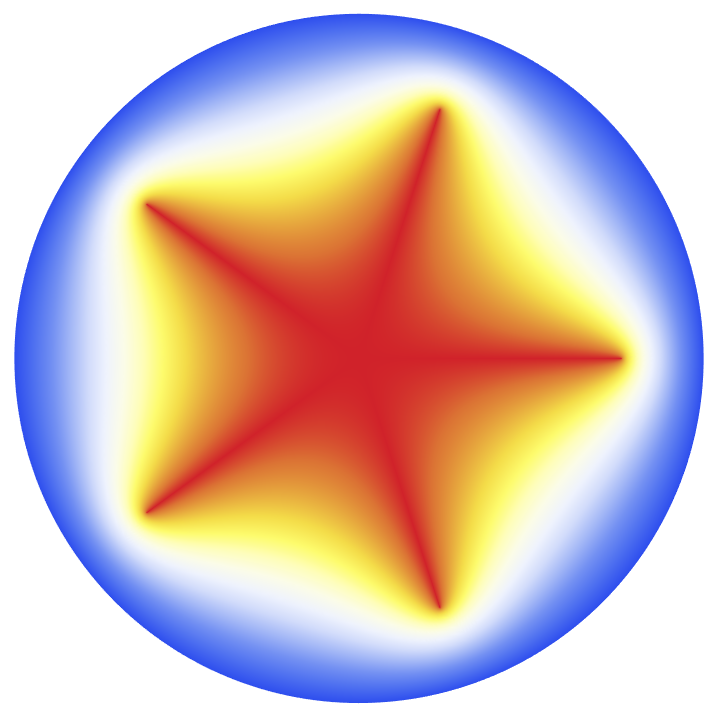
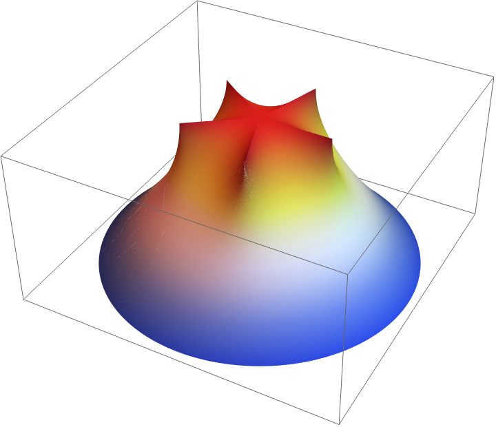
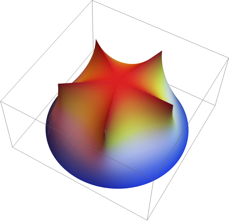
Figure 19: Five radial hyperbolic segments. Surface plots of the potentials in the lower limit cases when all segments meet at the origin.

(a)

(b)

Figure 20: Five radial hyperbolic segments. Error convergence: (A) Short segments, (B) Long segmenets. Both exact and estimated errors are shown in loglog-plots, $N$ is the number of degrees of freedom.

5.3 Constellation of six hyperbolic segments constrained to a disk

Analogously to the case with disks, we consider the positions of six hyperbolic segments that maximize the capacity $\operatorname{\mathrm{cap}}({\mathbb{D}},E)$ under the constraint that the hyperbolic centers of these disks are in the Euclidean disk $|z|\leq R$ (we assume in the examples below that $R=0.75$). The segments are numbered $E_{1}$ to $E_{6}$ in counterclockwise orientation. We denote the center of the disk $E_{j}$ by $z_{j}$, $j=1,\ldots,6$. Without loss of generality, we assume that the center $z_{1}$ of the segment $E_{1}$ is on the positive real axis.

First we assume that all six segments have equal hyperbolic length $=0.4$. The positions of these six segments that maximize the capacity $\operatorname{\mathrm{cap}}({\mathbb{D}},E)$ are on the Euclidean circle $|z|=R$ and such the hyperbolic distances between the centers of any two adjacent segments are equal (see Figure 21(A) and Table 7). When we change the hyperbolic length of one of these segments to be $0.8$ (see Figure 21(B)) or $1.6$ (see Figure 21(C)), then the centers of the other segments are moved away from the larger segment (see Table 7).

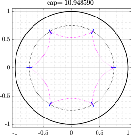
(a)

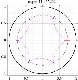
(b)

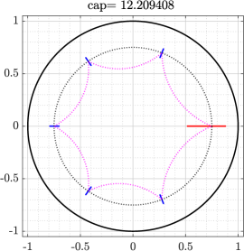
(c)

Figure 21: Segment $E_{1}$ has hyp-length $0.4$ (left), $0.8$ (center), and $1.6$ (right). Segments $E_{2}$ through $E_{6}$ have hyp-length $0.4$.

Table 7: The hyperbolic distance between the centers of consecutive segments in Figure 21.

Case	Capacity	$\rho(z_{1},z_{2})$	$\rho(z_{2},z_{3})$	$\rho(z_{3},z_{4})$	$\rho(z_{4},z_{5})$	$\rho(z_{5},z_{6})$	$\rho(z_{6},z_{1})$
A	$10.9486$	$2.6161$	$2.6161$	$2.6161$	$2.6161$	$2.6161$	$2.6161$
B	$11.4152$	$2.7080$	$2.5705$	$2.5655$	$2.5655$	$2.5705$	$2.7080$
C	$12.2094$	$2.8236$	$2.5089$	$2.4931$	$2.4931$	$2.5089$	$2.8236$

5.4 Constellation of five hyperbolic segments constrained to the real line

In the final experiment we consider the positions of five hyperbolic segments that maximize the capacity $\operatorname{\mathrm{cap}}({\mathbb{D}},E)$ under the constraint that the hyperbolic centers of these slits are in the interval $[-R,R]$ (we assume in the examples below that $R=0.75$). The segments are numbered (E1-E5) from left to right.

First all five segments are set to have equal hyperbolic length $=0.4$. The positions of these five segments that maximize the capacity $\operatorname{\mathrm{cap}}({\mathbb{D}},E)$ are shown in Figure 22 and the hyperbolic distance between the centers of any two adjacent segments is presented in Table 8. Then we change the hyperbolic length of one of these segments to be $0.8$. The obtained results are presented in Figure 22 and Table 8.

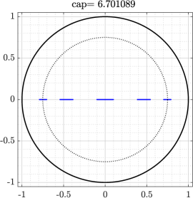
(a)

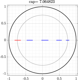
(b)

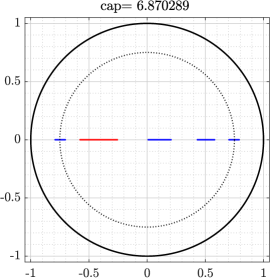
(c)

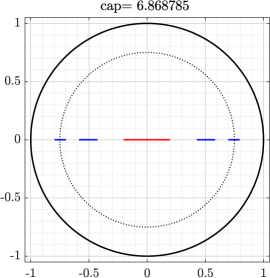
(d)

Figure 22: First row: All segments have hyp-length $0.4$. Second row: One segment with hyp-length $0.8$ (red) and four segments with hyp-length $0.4$ (blue).

Table 8: The hyperbolic distances between the centers of consecutive segments in Figure 22.

Case	Capacity	$\rho(z_{1},z_{2})$	$\rho(z_{2},z_{3})$	$\rho(z_{3},z_{4})$	$\rho(z_{4},z_{5})$
A	$6.7011$	$0.9293$	$1.0166$	$1.0166$	$0.9293$
B	$7.0648$	$1.1379$	$0.9521$	$0.9439$	$0.8579$
C	$6.8703$	$1.0317$	$1.1313$	$0.9071$	$0.8218$
D	$6.8688$	$0.8222$	$1.1237$	$1.1237$	$0.8222$

In all cases the results computed with BIE and FEM agree within the prescribed tolerance.

5.4.1 On Computational Costs

PDE-optimization is inherently expensive. In Table 9 performance data on the six disks maximization problem shown in Figure 1 is presented. In all cases the interior-point tolerance is the same, $\epsilon=10^{-6}$, and within the $hp$-FEM simulations, meshing is performed with the same discretization control in every evaluation. Not surprisingly, the overall conclusions are very similar to those drawn in our previous work [11], where minimization was considered. Comparison of the two methods is only qualitative, since both underlying hardware and the interior-point implementations are different.

The two implementations have very different requirements per iteration step. It is very likely that this is due to different numerical differentiation algorithms being used in Matlab and Mathematica. Observe that the number of iteration steps becomes comparable once the $hp$-solutions are sufficiently accurate, yet the number of evaluations is not. The average time for one evaluation in BIE is four to five times faster than one evaluation in $hp$-FEM. Matlab and Mathematica results have been computed on modern Intel and Apple Silicon computers, respectively.

In short, for optimal performance, the individual solutions must be accurate enough so that the error induced by numerical approximation of the gradients and Hessians is balanced with other sources of error. For BIE, the problem is practically fully resolved already at $n=2^{6}$, whereas for the $hp$-FEM it appears that the same mesh with $p=4$ is not adequate in comparison with the one at $p=8$. Even though the time spent in one individual iteration step is doubled, the overall time for $p=8$ is significantly lower.

Remark 1

In comparison with a similar minimization problems in [11], we observe that the constrained maximization problems are less resource intensive in terms of iteration steps and runtimes. This is more notable in the BIE results. Our interpretation is that in maximization the boundary components are relatively faraway from each other and hence high accuracy results can be obtained for moderate values of $n$ and few number of iterations.

Table 9: Solution times for the maximization process for the six hyperbolic disks in Figure 1. Number of steps is number of iterations in the interior-point algorithm. Number of evaluations is the total number of solves performed during the maximization.

Method	Discretization	Time	# of steps	# of evaluations
BIE	$n=2^{6}$	162.5	16	204
	$n=2^{8}$	274.7	17	216
	$n=2^{10}$	637.8	22	286
$hp$-FEM	$p=4$	21749.2	144	23706
	$p=6$	5132.6	24	3704
	$p=8$	2170.9	6	1050

6 Conclusions

Maximizing the conformal capacity of a constellation is opposite to minimizing studied in [11]. In [11] the main result was that the disks of the constellation group together in the local minima cases. Here we have shown that in the case of maximization the expected natural dispersion phenomenon occurs: the disks move as close to the unit circle as the constraints permit and, at the same time, the disks keep as far away from each other as possible. Replacing disks by other simple geometric objects also seems possible as our experiments with radial and rectilinear segments show.

A mathematical proof of the extremal cases we found in the experiments is missing. Heuristically one could say that in the case when the constellation disks are as far as possible from each other, the constellation capacity is nearly additive, equal to the sum of the capacities of the disks. This was studied in [4] and [16] from another point of view and similar conclusions obtained.

The study of this topic seems to offer many opportunities for later research. For example, one could study the above problems replacing the unit disk by some other domain, e.g. by a polygonal domain. Also one could investigate similar problems for other capacities such as the logarithmic and analytic capacities.

Code Availability

In the interest of reproducibility, the codes for our computations are available through the link https://github.com/mmsnasser/maxcap.

References

- [1] I. Babuška and B. Guo, Regularity of the solutions of elliptic problems with piecewise analytical data, parts I and II, SIAM J. Math. Anal., 19, (1988), 172–203 and 20, (1989), pp. 763–781.
- [2] A. Baernstein, Symmetrization in analysis. With David Drasin and Richard S. Laugesen. With a foreword by Walter Hayman. New Mathematical Monographs, 36. Cambridge University Press, Cambridge, 2019.
- [3] A. F. Beardon, The Geometry of Discrete Groups, Springer-Verlag, New York, 1983.
- [4] D. Betsakos, A. Solynin, and M. Vuorinen, Conformal capacity of hedgehogs. Conform. Geom. Dyn., 27 (2023), 55–97.
- [5] S.V. Borodachov, D.P. Hardin, and E.B. Saff, Discrete energy on rectifiable sets. Springer Monographs in Mathematics. Springer, New York, 2019.
- [6] P.D. Dragnev, B. Fuglede, D. P. Hardin, E.B. Saff, and N. Zorii, Constrained minimum Riesz energy problems for a condenser with intersecting plates. J. Anal. Math., 140 (2020), 117–159.
- [7] V.N. Dubinin, Condenser Capacities and Symmetrization in Geometric Function Theory, Birkhäuser, 2014.
- [8] F.W. Gehring, Inequalities for condensers, hyperbolic capacity, and extremal lengths. Michigan Math. J. 18 (1971), 1–20.
- [9] V.M. Goldshtein and Yu.G. Reshetnyak, Quasiconformal Mappings and Sobolev Spaces. Kluwer Academic Publishers Group, Dordrecht, 1990.
- [10] L. Greengard and Z. Gimbutas, FMMLIB2D: A MATLAB toolbox for fast multipole method in two dimensions, version 1.2. 2019, www.cims.nyu.edu/cmcl/fmm2dlib/fmm2dlib.html. Accessed 6 Nov 2020.
- [11] H. Hakula, M.M.S. Nasser, and M. Vuorinen, Mobile disks in hyperbolic space and minimization of conformal capacity. Electron. Trans. Numer. Anal., 60 (2024), 1–19.
- [12] H. Hakula, M. Neilan, and J. Ovall, A Posteriori Estimates Using Auxiliary Subspace Techniques, J. Sci. Comput. 72 no. 1 (2017), pp. 97–127.
- [13] H. Hakula, and T. Tuominen, Mathematica implementation of the high order finite element method applied to eigenproblems. Computing, (95) 1 (2013) 277–301.
- [14] P. Hariri, R. Klén, and M. Vuorinen, Conformally Invariant Metrics and Quasiconformal Mappings, Springer Monographs in Mathematics, Springer, Berlin, 2020.
- [15] J. Heinonen, T. Kilpeläinen, and O. Martio, Nonlinear Potential Theory of Degenerate Elliptic Equations, Dover Publications, New York, 2006.
- [16] E.M. Kalmoun, M.M.S. Nasser, and M. Vuorinen, Numerical computation of a preimage domain for an infinite strip with rectilinear slits. Adv. Comput. Math., 49 (2023), article number 5.
- [17] P. Koebe, Abhandlungen zur Theorie der konformen Abbildung, IV. Abbildung mehrfach zusammenhängender schlichter Bereiche auf Schlitzbe-reiche. Acta Math. 41 (1918), 305–344.
- [18] MATLAB, 2022a. 9.12 (R2022a), Natick, Massachusetts: The MathWorks Inc.
- [19] M.M.S. Nasser, Numerical conformal mapping of multiply connected regions onto the second, third and fourth categories of Koebe’s canonical slit domains. J. Math. Anal. Appl. 382 (2011), 47–56.
- [20] M.M.S. Nasser, Fast solution of boundary integral equations with the generalized Neumann kernel. Electron. Trans. Numer. Anal. 44 (2015), 189–229.
- [21] M.M.S. Nasser and C.C. Green, A fast numerical method for ideal fluid flow in domains with multiple stirrers. Nonlinearity 31 (2018), 815–837.
- [22] M.M.S. Nasser and M. Vuorinen, Numerical computation of the capacity of generalized condensers. J. Comput. Appl. Math. 377 (2020) 112865.
- [23] M.M.S. Nasser and M. Vuorinen, Isoperimetric properties of condenser capacity. J. Math. Anal. Appl. 499 (2021) 125050.
- [24] J. Nocedal and S. Wright, Numerical Optimization, Springer New York, NY, 2006.
- [25] G. Pólya and G. Szegö, Isoperimetric Inequalities in Mathematical Physics. Annals of Mathematics Studies, no. 27, Princeton University Press, Princeton, N. J., 1951.
- [26] Ch. Schwab, - and -Finite Element Methods, Oxford University Press, 1998.
- [27] A.Yu. Solynin and V. A. Zalgaller, An isoperimetric inequality for logarithmic capacity of polygons. Ann. of Math. (2) 159 (2004), no. 1, 277–303.
- [28] Wolfram Research, Inc., Mathematica, Version 14.0, Champaign, IL, 2024.