BAD-NEUS: Rapidly converging trajectory stratification

Abstract

An issue for molecular dynamics simulations is that events of interest often involve timescales that are much longer than the simulation time step, which is set by the fastest timescales of the model. Because of this timescale separation, direct simulation of many events is prohibitively computationally costly. This issue can be overcome by aggregating information from many relatively short simulations that sample segments of trajectories involving events of interest. This is the strategy of Markov state models (MSMs) and related approaches, but such methods suffer from approximation error because the variables defining the states generally do not capture the dynamics fully. By contrast, once converged, the weighted ensemble (WE) method aggregates information from trajectory segments so as to yield unbiased estimates of both thermodynamic and kinetic statistics. Unfortunately, errors decay no faster than unbiased simulation in WE. Here we introduce a theoretical framework for describing WE that shows that introduction of an element of stratification, as in nonequilibrium umbrella sampling (NEUS), accelerates convergence. Then, building on ideas from MSMs and related methods, we propose an improved stratification that allows approximation error to be reduced systematically. We show that the improved stratification can decrease simulation times required to achieve a desired precision by orders of magnitude.

I Introduction

The sampling of a stochastic process can be controlled by evolving an ensemble and splitting and merging the trajectories of its members, and various algorithms based on this strategy have been introduced [1, 2, 3, 4, 5, 6, 7]. Because the trajectory segments between splitting events are unbiased, such algorithms can yield dynamical statistics, such as transition probabilities and mean first passage times (MFPTs) to selected states, in addition to steady-state probability distributions and averages. Furthermore, splitting algorithms generally require little communication between the members of the ensemble, making them relatively straightforward to implement regardless of the underlying dynamics, and community software is available [8]. As a result, splitting algorithms are widely used.

Recent mathematical analysis of one of the oldest splitting algorithms in the molecular simulation literature, weighted ensemble (WE) [1], shows that it is asymptotically unbiased and can dramatically reduce the variance of statistics when the splitting criteria, which are based on a partition of the state space, are chosen appropriately [9]. However, the method relies on convergence of the steady-state ensemble of trajectories, which is known to be slow. In fact, as we argue below and was observed previously [9], it is as slow as running direct unbiased simulations. Prior to convergence, the method is systematically biased.

Some previous work to accelerate the convergence of WE focused on improving the initialization of walkers using an approximation of the stationary distribution. In one case, the approximation of the stationary distribution was obtained from a free-energy method that biased trajectories to escape metastable wells [10], while in another it was obtained from a machine-learning method based on unbiased short trajectories [11]. The former approach requires the underlying dynamics to obey detailed balance to ensure the validity of the free energy method, while the latter approach relies on a Markov approximation (but does not make other restrictions on the dynamics). In both cases, however, the approximation to the stationary distribution is used only for the first iteration, and so if the approximation is deficient, significant bias can persist in the WE calculation for many iterations.

Others focused on improving the rate estimates from WE [12, 13]. Of particular relevance to the present study, Copperman and Zuckerman exploited the fact that splitting algorithms sample unbiased trajectory segments to construct history-augmented Markov state models (haMSMs) [14] from their WE data [12]. In an haMSM, the system is divided into discrete states and the probabilities for transitions between them are computed from data, just as in a standard MSM, except that the path ensemble is split based on the last metastable state visited; the rate constant is then computed as the flux from $A$ to $B$ conditioned on having last visited $A$, normalized by the steady-state probability of having last visited $A$. The idea is that finer discretization of the state space than the WE simulation yields improved estimates. However, this approach does not accelerate the convergence of the sampling.

The basic approach in our work is to combine these strategies and fully integrate them in the sampling algorithm by applying a short-trajectory based approximation to the stationary distribution between successive iterations. As we show below, if the approximation satisfies certain properties and is correctly integrated in the algorithm, we can accelerate the convergence by several orders of magnitude without introducing systematic bias. Our approach is able to compute the full stationary distribution with minimal assumptions about the dynamics, as well as kinetic statistics such as rates and committors (probabilities of visiting selected states before others).

Conceptually, one can view our approach as a form of stratification, in which the weights of not just individual trajectory segments but groups of them are manipulated. Stratification was first introduced for controlling the sampling of trajectory segments in nonequilibrium umbrella sampling (NEUS) [3, 15, 16, 4, 17, 18]. NEUS groups trajectories that are in the same regions of state space, as defined by collective variables (CVs), and estimates the steady-state probabilities of the regions by solving a global flux balance equation; this strategy was subsequently adopted in extensions of WE[19] and exact milestoning (EM)[6]. A unified framework for trajectory stratification that incorporates elements of all of the above algorithms and is unbiased in the limit that each region contains an infinite number of ensemble members is presented in Ref. 18, which also shows that the regions can be defined in terms of path-based quantities. Mathematical analysis of trajectory stratification algorithms can be found in Refs. 20, 21.

Our paper is organized as follows. In Section II, we review the WE algorithm and recast it to show why an initialization bias is slow to disappear. This formulation also clarifies the relation of WE to the NEUS algorithm as described in Ref. 18, and we show how software for WE can be easily extended to enable trajectory stratification in Section III. In Section IV, we introduce a generalization of MSMs that represents the dynamics through a basis expansion [22, 23, 24] and in turn our strategy for accelerating sampling, which we term Basis-Accelerated NEUS (BAD-NEUS). We show that the NEUS algorithm is a special case of our new scheme. In Sections V and VI, we demonstrate BAD-NEUS on a two-dimensional model with a known steady-state distribution and a molecular example.

II Weighted Ensemble (WE)

As described above, in WE, the state space is partitioned into regions, and then trajectories are copied (cloned or split) or removed (killed or pruned) from the ensemble based on criteria. Mathematically, we denote the state of ensemble member (henceforth, walker) $i$ at time $t$ by $X^{i}_{t}$, and we associate with $i$ a weight $w^{i}_{t}$ such that $\sum_{i}w^{i}_{0}=1$. We track the index of the region containing $X^{i}_{t}$ by an index process $J^{i}_{t}$. For example, $J^{i}_{t}$ might track the element of a partition of state space in which $X^{i}_{t}$ currently resides. Other options for the index process are available and can be advantageous (see Refs. 18, 25 for further discussion).

Here, we use a relatively simple procedure and represent the splitting and pruning by resampling the ensemble within each region. Each iteration of the sampling thus consists of two steps: evolution according to the underlying dynamics and resampling the ensemble. In the evolution step, for each walker $i$, we numerically integrate for a time interval $\Delta$ to obtain $X^{i}_{t+\Delta}$ from $X^{i}_{t}$ and update $J^{i}_{t+\Delta}$ accordingly. In this step the weights are unchanged; $w^{i}_{t+\Delta}=w^{i}_{t}$. We note that $\Delta$ can be a random stopping time, not just a fixed time interval. An often useful choice is to take $t+\Delta$ to be the first time after time $t$ that the value of the index process $J^{i}$ changes. In this case, each walker has a different value for $\Delta.$ In the resampling step, for each value $k$ of the index process (e.g., for each region in a partition of state space), if there is at least one walker with $J^{i}_{t+\Delta}=k$, we select a number $N_{k}$. Then we sample from the set $\Phi=\{i:J^{i}_{t+\Delta}=k\}$ $N_{k}$ times with replacement according to the probabilities $p_{i}=w^{i}_{t+\Delta}/\sum_{i\in\Phi}w^{i}_{t+\Delta}$. For each index $r$ so chosen, we append $(X^{r}_{t+\Delta},J^{r}_{t+\Delta},\sum_{i\in\Phi}w^{i}_{t+\Delta}/N_{k})$ to the new ensemble.

If the underlying dynamics are ergodic, in the case where $\Delta$ is a fixed time horizon, WE can be used to compute steady-state averages of functions as

$$\mathbbm{E}_{X_{0}\sim\pi}[g(X_{0},X_{1},\ldots,X_{\Delta-1})]\\ =\lim_{T\to\infty}\frac{1}{T}\sum_{n=0}^{T}\frac{1}{N}\sum_{i=0}^{N}g(X^{i}_{n\Delta},X^{i}_{n\Delta+1},\ldots,\\ X^{i}_{n\Delta+\Delta-1})w^{i}_{n\Delta},$$ (1)

where the subscript on the expectation indicates that we draw the initial state $X_{0}$ from the steady-state distribution $\pi,$ and $n$ indexes successive weighted ensemble iterations. We present necessary modifications for the case where $\Delta$ is a random variable later. Here and below, $X$ without a superscript indicates a realization of the underlying Markov process rather than a walker in an ensemble. An important example is the steady-state flux into a set $D$ of interest, which can be used to compute the MFPT to $D$ from another set in the right algorithmic setup [9]. This flux can be obtained by setting $g(X_{0},\ldots,X_{\Delta})=\mathbbm{1}_{D^{c}}(X_{0})\mathbbm{1}_{D}(X_{1})$, where $\mathbbm{1}_{D}(x)$ is an indicator function that is 1 if $x\in D$ and 0 otherwise. This amounts to counting the number of walkers that enter $D$ in a single time step and summing the total weight of those walkers.

Having stated the basic WE algorithm, we now present WE in a new way. While this may initially appear to complicate the description, it reveals that WE is slow to converge and facilitates the introduction of approaches to accelerate convergence. In this description, which we call the distribution representation of WE, we directly evolve distributions rather than approximating them through individual walkers. To this end, we define the flux distributions

$$\overline{\pi}_{\ell}(dx|k)=P[X_{S(\ell)}\in dx|J_{S(\ell)}=k]$$ (2)

where $dx$ is an infinitesimal volume in state space that is located at a specific value of $x$ and $S(\ell)$ is an increasing sequence of stopping times. For example, if we choose $S(\ell)=\ell\Delta$ for a fixed $\Delta$, the following description corresponds to the standard version of WE already sketched. Alternatively, we can let $S(\ell)$ be the time of the $\ell$-th change in the value of the index process $J$:

$$S(0) =0$$ (3)

$$S(1) =\min\{t>0:J_{t}\neq J_{t-1}\}$$

$$\vdots$$

$$S(\ell) =\min\{t>S(\ell-1):J_{t}\neq J_{t-1}\}.$$

In all practical implementations of the sampling algorithms that we discuss, the conditional flux distributions take the form of empirical distributions of $N$ walkers:

$$\overline{\pi}_{\ell}(dx|k)\approx\frac{1}{\overline{z}_{\ell}^{k}}\sum_{i=1}^{N}w_{S^{i}(\ell)}^{i}\delta_{X_{S^{i}(\ell)}^{i}}(dx)\mathbbm{1}_{\{k\}}\left(J_{S^{i}(\ell)}^{i}\right),$$ (4)

where $\delta_{x}$ is the Dirac delta function centered at position $x$, and the normalization constant $\overline{z}_{\ell}^{k}$ is the total weight in region $k$ at time $S(\ell)$:

$$\overline{z}_{\ell}^{k} =P[J_{S(\ell)}=k]\approx\sum_{i=1}^{N}w_{S^{i}(\ell)}^{i}\mathbbm{1}_{\{k\}}\left(J_{S^{i}(\ell)}^{i}\right).$$ (5)

The outputs of the weighted ensemble iteration and the accelerated variants that we consider here are approximations of the steady-state conditional flux distributions, as well as estimates of the corresponding normalization constants. The conditional flux distributions are related to joint flux distributions through the normalization constants:

$$\overline{\pi}_{\ell}(dx,k) =P[X_{S(\ell)}\in dx,J_{S(\ell)}=k]$$ (6)

$$=\overline{z}_{\ell}^{k}\overline{\pi}_{\ell}(dx|k),$$ (7)

and we work with $\overline{\pi}_{\ell}(dx,k)$ below.

In particular, we now write the evolution and resampling steps in terms of operators. For the former, we define the operator $\mathcal{U}$, which propagates the joint flux distribution of $(X_{S(\ell)},J_{S(\ell)})$ for a duration of $S(\ell+1)-S(\ell)$:

$$\mathcal{U}\overline{\pi}_{\ell}(dx,k)=\overline{\pi}_{\ell+1}(dx,k).$$ (8)

In the long-time limit, this yields the eigenequation

$$\overline{\pi}(dx,k)=\mathcal{U}\overline{\pi}(dx,k),$$ (9)

where $\overline{\pi}$ is the steady-state joint flux distribution. In practice, one approximates the distributions through walkers, and we denote the corresponding evolution by $\tilde{\mathcal{U}}$. Mathematically,

$$\tilde{\mathcal{U}}\left[\frac{1}{N}\sum_{i=1}^{N}w_{S^{i}(\ell)}^{i}\delta_{X_{S^{i}(\ell)}^{i}}(dx)\mathbbm{1}_{\{k\}}\left(J_{S^{i}(\ell)}^{i}\right)\right]\\ =\frac{1}{N}\sum_{i=1}^{N}w_{S^{i}(\ell)}^{i}\delta_{X_{S^{i}(\ell+1)}^{i}}(dx)\mathbbm{1}_{\{k\}}\left(J_{S^{i}(\ell+1)}^{i}\right).$$ (10)

The subscript on the weight does not change because the evolution step only affects the state and index of a walker, not its weight. $\tilde{\mathcal{U}}$ as defined in (10) is an unbiased stochastic approximation of $\mathcal{U}$ in the sense that, for any function $g$ and any distribution $\rho$,

$$\sum_{k}\int g(x,k)[\mathcal{U}\rho](dx,k)=\\ \mathbbm{E}\left[\sum_{k}\int g(x,k)[\tilde{\mathcal{U}}\rho](dx,k)\right].$$ (11)

If distributions are represented with some ansatz such as a neural network, one can also apply an approximate propagator based on a variational method as outlined in Refs. 26, 27. Such a scheme would not require new trajectories to be run at each iteration, nor would it require a resampling step.

As noted above, we also represent resampling through an operator, $\mathcal{R}_{k}$. We define it such that, for any distribution $\rho$ and any function $g$

$$\sum_{j}\int g(x,j)\left(\frac{1}{\zeta_{k}}\mathbbm{1}_{\{k\}}(j)\rho(dx,j)\right)=\\ \mathbbm{E}\left[\sum_{j}\int g(x,j)\mathcal{R}_{k}\rho\right]$$ (12)

and

$$\zeta_{k}=\sum_{j}\int\mathbbm{1}_{\{k\}}(j)\rho(dx,j).$$ (13)

Above, the LHS selects the portion of the distribution $\rho$ in region $k$ and then renormalizes it, while the RHS corresponds to resampling from the distribution. A simple choice which is commonly employed for the operator $\mathcal{R}_{k}$ is to sample the set of walkers in region $k$ at the end of the evolution (denoted $K$) from a multinomial distribution with probability proportional to $\{w_{S^{i}(\ell)}^{i}\mathbbm{1}_{\{k\}}(J_{S^{i}(\ell)}^{i})\}_{i\in K}$ with $N_{k}$ trials and then return the distribution

$$\mathcal{R}_{k}\left[\frac{1}{N}\sum_{i=1}^{N}w_{S^{i}(\ell)}^{i}\delta_{X_{S^{i}(\ell)}^{i}}(dx)\mathbbm{1}_{\{k\}}(J_{S^{i}(\ell)}^{i})\right]\\ =\frac{1}{N_{k}}\sum_{i\in K}\delta_{X_{S^{i}(\ell)}^{i}}(dx)$$ (14)

and normalization

$$\overline{z}_{\ell}^{k}\approx\sum_{i}\mathbbm{1}_{\{k\}}(J_{S^{i}(\ell)}^{i})w_{S^{i}(\ell)}^{i}.$$ (15)

In words, (14) shows that ${\cal R}_{k}$ constructs the state distribution from a sum over the resampled walkers in each region. There are other possible ways of resampling in the walker representation, such as stratified or pivotal resampling [28], and these may in practice be better. However, any choice that satisfies (12) suffices for our discussion.

Finally, we connect the flux distributions $\overline{\pi}(dx|k)$ to the steady-state distribution $\pi(x,k)$ for the process $(X_{t},J_{t})$, where the absence of superscripts again indicates the underlying Markov process rather than a walker in an ensemble. We do this with a key identity, which we now state. For a function $g$ of a length $\tau$ trajectory,

$$\mathbbm{E}_{(x,k)\sim\pi}[g(X_{0},J_{0},\dots,X_{t},J_{t})]=\frac{\sum_{k}\overline{z}^{k}\int\overline{\pi}(dx|k)\mathbbm{E}_{X_{0}=x,J_{0}=k}\left[\sum_{t=0}^{S(1)-1}g(X_{t},J_{t},\dots,X_{t+\tau},J_{t+\tau})\right]}{\sum_{k}\overline{z}^{k}\int\overline{\pi}(dx|k)\mathbbm{E}_{X_{0}=x,J_{0}=k}\left[S(1)\right]},$$ (16)

where now $\pi$ is the steady-state joint distribution of $(X_{t},J_{t})$. This identity says that, for each region $k$, we draw initial walker states $X_{0}$ from $\overline{\pi}(dx|k)$ and set $J_{0}=k$; we evolve those walkers until they leave region $k$; then we compute averages over them and weight the contribution from the walkers that started in region $k$ by $\overline{z}^{k}$, which is the steady-state limit of $\overline{z}_{\ell}^{k}$. We derive (16) in Appendix A. The distribution representation of WE is summarized in Algorithm 1.

Algorithm 1 WE (distribution representation)

1: Approximate Markov propagator $\tilde{\mathcal{U}}$, resampling operator $\mathcal{R}_{k}$, starting flux distributions $\{\overline{\pi}_{0}(dx|k)\}_{k=1}^{n}$, initial region weights $\{\overline{z}_{0}^{k}\}_{k=1}^{n}$ with $\sum_{k}\overline{z}_{0}^{k}=1$.

2:for $\ell=0,\dots,L$ do

3:     $\overline{\pi}_{\ell}(dx,k)\leftarrow\overline{z}_{\ell}^{k}\overline{\pi}_{\ell}(dx|k)$

4:     $\tilde{\overline{\pi}}\leftarrow[\tilde{\mathcal{U}}\overline{\pi}_{\ell}](dx,k)$ $\triangleright$ One Power Iteration Step

5:     for $k=1,\dots,n$ do

6:         $\overline{\pi}_{\ell+1}(dx|k),\overline{z}_{\ell+1}^{k}\leftarrow\mathcal{R}_{k}[\tilde{\overline{\pi}}]$

7:     end for

8:end for

9:return $\overline{\pi}_{L}(dx|k)$ and $\overline{z}_{L}^{k}$

We see that each step of WE applies the operator $\mathcal{U}$ to the previous distribution $\overline{\pi}_{\ell}(dx,k)$. Therefore, WE can be seen as performing a power iteration in ${\cal U}$, starting from some initial distribution. The resampling step in WE plays a role analogous to the normalization step in standard power iteration in the following sense. In standard power iteration, the normalization step serves to prevent the iterate from becoming too small or too large and introducing numerical instability. In WE, the resampling step serves to prevent any of the region distributions from becoming poorly sampled, which would increase variance. However, the normalization step in power iteration and, in turn, the resampling step in WE does not accelerate decay of initialization bias, nor is the WE autocorrelation time reduced relative to direct sampling.

Algorithm 1 suggests that, if $\tilde{\overline{\pi}}=\overline{\pi}$ in step 3, convergence would be achieved. Therefore, our strategy for accelerating WE is to replace the power iteration step with a more accurate approximation. Specifically, we compute changes of measure $\nu_{\ell}$ such that

$$\overline{\pi}(dx,k)\approx\nu_{\ell}(x,k)\overline{\pi}_{\ell}(dx,k).$$ (17)

If we set up our approximation such that whenever $\pi_{\ell}=\pi$, we get $\nu_{\ell}=1$, then the resulting modification of WE will have a fixed point at the true steady-state distribution, and there will be no approximation error resulting from deficiencies in the approximation algorithm’s specific ansatz. Our scheme has the advantage that it can potentially approach steady state much faster than WE. This is the idea that we develop in Sections III and IV.

III Nonequilibrium umbrellla sampling (NEUS)

We now present NEUS as a simple extension to WE that accelerates convergence in the way suggested in (17); EM [6] can be formulated similarly. Our development is based on the algorithm in Ref. 18, which corrects a small systematic bias in earlier NEUS papers [3, 15, 16, 4, 17]. We begin by making the observation that, at steady state,

$$\mathbbm{E}_{X_{0}\sim\overline{\pi}}[\mathbbm{1}_{\{k\}}(J_{0})]=\mathbbm{E}_{X_{0}\sim\overline{\pi}}[\mathbbm{1}_{\{k\}}(J_{S(1)})],$$ (18)

or, in terms of the density we wish to compute,

$$\int\overline{\pi}(dx,k)=\sum_{j}\int\overline{\pi}(dx,j)\mathbbm{E}_{X_{0}=x,J_{0}=j}[\mathbbm{1}_{\{k\}}(J_{S(1)})].$$ (19)

This observation introduces one equation per possible value of the index $j$. Therefore, we can parameterize the change of measure with as many free parameters:

$$\overline{\pi}(dx,k)\approx c_{\ell}^{k}\overline{z}_{\ell}^{k}\overline{\pi}_{\ell}(dx|k)$$ (20)

Substituting this ansatz into (19) and simplifying yields the matrix equation

$$c_{\ell}^{k}\overline{z}_{\ell}^{k}=\sum_{j}c_{\ell}^{j}\overline{z}_{\ell}^{j}\overline{G}_{jk},$$ (21)

where

$$\overline{G}_{jk}=\int\overline{\pi}(dx|j)\mathbbm{E}_{X_{0}=x,J_{0}=j}[\mathbbm{1}_{\{k\}}(J_{S(1)})].$$ (22)

We summarize NEUS in Algorithm 2.

Algorithm 2 NEUS

1: Approximate Markov propagator $\tilde{\mathcal{U}}$, Resampling operator $\mathcal{R}_{k}$, starting flux distributions $\{\overline{\pi}_{0}(dx|k)\}_{k=1}^{n}$, initial region weights $\{\overline{z}_{0}^{k}\}_{k=1}^{n}$ with $\sum_{k}\overline{z}_{0}^{k}=1$.

2:for $\ell=0,\dots,L$ do

3:     $\overline{G}_{jk}\leftarrow\int\overline{\pi}_{\ell}(dx|j)\mathbbm{E}_{X_{0}=x,J_{0}=j}[\mathbbm{1}_{\{k\}}(J_{S(1)})]$

4:     Solve $c_{\ell}\overline{z}_{\ell}\overline{G}=c_{\ell}\overline{z}_{\ell}$ for $c_{\ell}\overline{z}_{\ell}$

5:     $\overline{\pi}_{\ell}(dx,k)\leftarrow c_{\ell}^{k}\mathbbm{1}_{\{k\}}\overline{z}_{\ell}^{k}\overline{\pi}_{\ell}(dx|k)$

6:     $\tilde{\overline{\pi}}\leftarrow\tilde{\mathcal{U}}\overline{\pi}_{\ell}(dx,k)$

7:     for $k=1,\dots,n$ do

8:         $\overline{\pi}_{\ell+1}(dx|k),\overline{z}_{\ell+1}^{k}\leftarrow\mathcal{R}_{k}[\tilde{\overline{\pi}}]$

9:     end for

10:end for

11:return $\overline{\pi}_{L}(dx|k)$ and $\overline{z}_{L}^{k}$

We thus see that NEUS is distinguished from WE by steps 2 and 3. In practice, walkers are drawn and their dynamics are simulated to determine $S(\ell+1)$ in the loop over $\ell$ prior to step 2 (the resulting state distribution is used later in step 5); then, $\overline{G}_{jk}$ is computed in step 2 from walkers at iteration $\ell$ as

$$\overline{G}_{jk}\approx\frac{\sum_{i}\mathbbm{1}_{\{j\}}\left(J^{i}_{S^{i}(\ell)}\right)\mathbbm{1}_{\{k\}}\left(J^{i}_{S^{i}(\ell+1)}\right)}{\sum_{i}\mathbbm{1}_{\{j\}}\left(J^{i}_{S^{i}(\ell)}\right)}.$$ (23)

We solve for the product $c_{\ell}\overline{z}_{\ell}$ directly and update the approximation for $\overline{\pi}$ accordingly. We then proceed as in WE.

We note that, if the flux distributions $\overline{\pi}(dx|k)$ and normalization constants $\overline{z}^{k}$ assume their steady-state values, then (21) is satisfied by $c^{k}=1$, and NEUS has the correct fixed point.

IV BAD-NEUS

To improve on NEUS, it is necessary to improve the approximation of the change of measure in (17). Here we do so by introducing a basis expansion. This allows us to vary the expressivity of the approximation through the number of basis functions, which can exceed the number of regions, in contrast to the steady-state condition in (18).

To this end, we note that, for any lag time $\tau$ and any function $f(x,k)$,

$$\mathbbm{E}_{(X_{0},J_{0})\sim\pi}[f(X_{0},J_{0})-f(X_{\tau},J_{\tau})]=0.$$ (24)

We stress that this relation holds for any fixed time $\tau$. Expanding this expectation using (16), with $g(X_{0},J_{0},\dots,X_{\tau},J_{\tau})=f(X_{0},J_{0})-f(X_{\tau},J_{\tau})$ and multiplying through by the normalization in the denominator, we obtain

$$0=\sum_{k}\overline{z}^{k}\int\overline{\pi}(dx|k)\mathbbm{E}_{X_{0}=x,J_{0}=k}\left[\sum_{t=0}^{S(1)-1}f(X_{t},J_{t})-f(X_{t+\tau},J_{t+\tau})\right].$$ (25)

We then introduce the basis set $\{\phi_{p}(x,k)\}_{p}$, and write

$$\overline{\pi}(dx,k)=\overline{z}^{k}\overline{\pi}(dx|k)\approx\sum_{p}c_{\ell}^{p}\phi_{p}(x,k)\overline{z}_{\ell}^{k}\overline{\pi}_{\ell}(dx|k).$$ (26)

Making the choice $f=\phi_{r}$ and inserting the basis expansion into (25) gives

$$0=\sum_{kp}c_{\ell}^{p}\overline{z}_{\ell}^{k}\int\phi_{p}(x,k)\overline{\pi}_{\ell}(dx|k)\mathbbm{E}_{X_{0}=x,J_{0}=k}\left[\sum_{t=0}^{S(1)-1}\phi_{r}(X_{t},J_{t})-\phi_{r}(X_{t+\tau},J_{t+\tau})\right].$$ (27)

This is a linear system which can be solved for the expansion coefficients:

$$0=\sum_{p}c_{\ell}^{p}M_{pr}.$$ (28)

with the matrix entries given by

$$M_{pr}=\sum_{k}\overline{z}_{\ell}^{k}\int\phi_{p}(x,k)\overline{\pi}_{\ell}(dx|k)\mathbbm{E}_{X_{0}=x,J_{0}=k}\left[\sum_{t=0}^{S(1)-1}\phi_{r}(X_{t},J_{t})-\phi_{r}(X_{t+\tau},J_{t+\tau})\right].$$ (29)

The basis set must include the constant function in its span so that the system has a unique nontrivial solution. The NEUS algorithm corresponds to the choice

$$\phi_{p}(x,k)=\mathbbm{1}_{\{p\}}(k)$$ (30)

and $\tau=1$. We summarize the BAD-NEUS algorithm in Algorithm 3.

Consistent with WE and NEUS, in practice, we estimate the integral $M_{pr}$ through a sum over walkers:

$$M_{pr}\approx\sum_{ki}\overline{z}_{\ell}^{k}\phi_{p}(X^{i}_{S^{i}(\ell)},k)\mathbbm{1}_{\{k\}}(J^{i}_{0})\left[\sum_{t=S^{i}(\ell)}^{S^{i}(\ell+1)-1}(\phi_{r}(X^{i}_{t},J_{t}^{i})-\phi_{r}(X^{i}_{t+\tau},J_{t+\tau}^{i}))\right].$$ (31)

Given $M$ and, in turn, the estimated expansion coefficients, we update the weights as

$$w_{S^{i}(\ell)}^{i}=\frac{\overline{z}_{\ell}^{J_{S^{i}(\ell)}^{i}}}{Z}\sum_{p}c_{\ell}^{p}\phi_{p}\left(X_{S^{i}(\ell)}^{i},J_{S^{i}(\ell)}^{i}\right),$$ (32)

where $Z$ normalizes the total of the walker weights to one. If the basis set contains the constant function in its span, and the flux distributions $\overline{\pi}_{\ell}(dx|k)$ and region weights $\overline{z}_{\ell}^{k}$ take their steady-state values, then the linear system (27) is solved by $\sum_{p}c_{p}\phi(x,k)=1$, and BAD-NEUS has the correct fixed point. To reduce variance in our estimate of the matrix $M$ to ensure a stable solve, it is often useful to work with the mixture distribution for the last $h$ iterations:

$$\overline{\pi}_{\ell,h}(dx|k)=\frac{1}{h}\sum_{t=\ell-h+1}^{\ell}\overline{\pi}_{t}(dx|k).$$ (33)

When working with walkers, this mixture distribution corresponds to concatenating the walkers from $h$ prior iterations, and therefore contains more data than using a single iteration. We simply substitute $\overline{\pi}_{\ell}$ for $\overline{\pi}_{\ell,h}$ in all of our algorithms. A unified walker-based algorithm that we use in practice is given in Algorithm 4, with the additional steps needed for NEUS and BAD-NEUS in Algorithm 5.

Finally, we note that the general strategy of improving the approximation of the change of measure is not limited to using a basis expansion. Just as one can use various means to solve the equations of the operator that encodes the statistics of the dynamics [22, 23, 29, 27], one can represent the change of measure here by either a basis expansion or a nonlinear representation. In particular, our tests based on the neural-network approach in Ref. 27 show significant promise (unpublished results).

Algorithm 3 BAD-NEUS

1: Approximate Markov propagator $\tilde{\mathcal{U}}$, Resampling operator $\mathcal{R}_{k}$, starting flux distributions $\{\overline{\pi}_{0}(dx|k)\}_{k=1}^{n}$, initial region weights $\{\overline{z}_{0}^{k}\}_{k=1}^{n}$ with $\sum_{k}\overline{z}_{0}^{k}=1$, basis set $\{\phi_{p}(x,k)\}_{p}$, lag time $\tau$

2:for $\ell=0,\dots,L$ do

3:     $\overline{\pi}_{\ell}\leftarrow\overline{\pi}_{\ell,h}$

4:     $\Delta\phi\leftarrow\sum_{t=0}^{S(1)-1}\phi_{r}(X_{t},J_{t})-\phi_{r}(X_{t+\tau},J_{t+\tau})$

5:     $M_{pr}\leftarrow\sum_{k}\int\overline{z}_{\ell}^{k}\phi_{p}(x,k)\overline{\pi}_{\ell}(dx|k)\mathbbm{E}_{X_{0}=x,J_{0}=k}\left[\Delta\phi\right]$

6:     Solve $cM=0$

7:     $\overline{\pi}_{\ell}(dx,k)\leftarrow\sum c_{\ell}^{p}\phi_{p}(x,k)\overline{z}_{\ell}^{k}\overline{\pi}_{\ell}(dx|k)$

8:     $\tilde{\overline{\pi}}\leftarrow\tilde{\mathcal{U}}\overline{\pi}_{\ell}(dx,j)$

9:     for $k=1,\dots,n$ do

10:         $\overline{\pi}_{\ell+1}(dx|k),\overline{z}_{\ell+1}^{k}\leftarrow\mathcal{R}_{k}[\tilde{\overline{\pi}}]$

11:     end for

12:end for

13:return $\overline{\pi}_{L}(dx|k)$ and $\overline{z}_{L}^{k}$

Algorithm 4 Trajectory Stratification (walker representation)

1: Starting ensemble of walkers $E_{0}=\{(X_{0}^{i},J_{0}^{i},w_{0}^{i})\}_{i=1}^{N},$ with $\sum_{i=1}^{N}w_{0}^{i}=1$, number of past iterations to retain $h$, total iterations $L,$ number of strata $n.$ lag time $\tau$

2:for $\ell=0,\dots,L$ do

3:     $N\leftarrow\text{length}(E_{\ell})$

4:     Generate a list of trajectories $T_{\ell}\leftarrow\{[(X_{S^{i}(\ell)}^{i},J_{S^{i}(\ell)}^{i},w_{S^{i}(\ell)}^{i}),(X_{S^{i}(\ell)+1}^{i},J_{S^{i}(\ell)+1}^{i},w_{S^{i}(\ell)}^{i}),\dots,$$(X_{S^{i}(\ell+1)+\tau}^{i},J_{S^{i}(\ell+1)+\tau}^{i},w_{S^{i}(\ell)}^{i})]\}_{i=1}^{N}$, where $(X_{S^{i}(\ell)}^{i},J_{S^{i}(\ell)}^{i},w_{S^{i}(\ell)}^{i})=E_{\ell}[i]$

5:     $T_{\ell}\leftarrow\text{concatenate}(\{T_{\ell},T_{\ell-1},\dots T_{\ell-h+1}\})$

6:     $N\leftarrow\text{length}(T_{\ell})$

7:     Renormalize the weights in $T_{\ell}$ by dividing each by $h$.

8:     Update weights $\{w^{i}_{S^{i}(\ell)}\}_{i=1}^{N}$ using Algorithm 5. (Omit for Weighted Ensemble)

9:     Initialize an empty list $E_{\ell+1}=\{\}$

10:     for $k=1,\dots,n$ do

11:         $\overline{z}^{k}_{\ell+1}\leftarrow\sum_{i=1}^{N}w_{S^{i}(\ell)}^{i}\mathbbm{1}_{\{k\}}(J^{i}_{S^{i}(\ell+1)})$

12:         for $r=1,\dots,N_{k}$ do

13:              Sample an index $b$ with probability proportional to $w_{S^{b}(\ell)}^{b}\mathbbm{1}_{\{k\}}(J^{b}_{S^{b}(\ell+1)})$

14:              Append to $E_{\ell}$ the configuration $(X_{S^{b}(\ell+1)}^{b},J_{S^{b}(\ell+1)}^{b},\overline{z}^{k}_{\ell+1}/N_{k})$

15:         end for

16:     end for

17:end for

18:return $T_{L}$ and $\overline{z}_{L}^{k}$

Algorithm 5 Approximating the steady-state flux distribution (walker representation)

1: List of trajectories $T_{\ell}$, lag time $\tau$, basis functions $\phi_{p}$, bin weights $\overline{z}_{\ell}$

2:$M_{pr}\leftarrow\sum_{ki}\overline{z}_{\ell}^{k}\phi_{p}(X^{i}_{S^{i}(\ell)},k)\mathbbm{1}_{\{k\}}(J^{i}_{0})\left[\sum_{t=S^{i}(\ell)}^{S^{i}(\ell+1)-1}(\phi_{r}(X^{i}_{t},J_{t}^{i})-\phi_{r}(X^{i}_{t+\tau},J_{t+\tau}^{i}))\right]$

3:Solve $c_{\ell}M=0$

4:$w_{S^{i}(\ell)}^{i}\leftarrow(\overline{z}_{\ell}^{J_{S^{i}(\ell)}^{i}}/Z)\sum_{p}c_{\ell}^{p}\phi_{p}\left(X_{S^{i}(\ell)}^{i},J_{S^{i}(\ell)}^{i}\right)$

5:return $\{w_{S^{i}(\ell)}^{i}\}_{i=1}^{N}$

V Two-dimensional test system

We first illustrate our approach by sampling a two-dimensional system, which enables us to compare estimates of the steady-state distribution to the Boltzmann probability to ensure that simulations are run until convergence. Specifically, the system $x=(u,v)$ is defined by the Müller-Brown potential [30], which is a sum of four Gaussian functions:

$$V(u,v)=\frac{1}{20}\sum_{i=1}^{4}C_{i}\exp[a_{i}(u-v_{i})^{2}\\ +b_{i}(u-u_{i})(v-v_{i})+c_{i}(v-v_{i})^{2}].$$ (34)

For all results shown, we use $C_{i}=\{-200,-100,-170,15\}$, $a_{i}=\{-1,-1,-6.5,0.7\}$, $b_{i}=\{0,0,11,0.6\}$, $c_{i}=\{-10,-10,-6.5,0.7\}$, $u_{i}=\{1,-0.27,-0.5,-1\}$, $v_{i}=\{0,0.5,1.5,1\}$. The potential with these parameter choices is shown in Figure 1. The presence of multiple metastable states and a minimum energy pathway that does not parallel the axes of the variables used for the numerical integration make this system representative of difficulties commonly encountered in molecular simulations. Because the model is two-dimensional, we can readily visualize results and compare them with statistics independently computed using the grid-based scheme in Ref. 27.

We evolve the system with overdamped Langevin dynamics, discretized with the BAOAB algorithm [31]:

$$X_{t+dt}=X_{t}-\nabla V(X_{t})dt+\sqrt{\frac{dt}{2\beta}}(Z_{t}+Z_{t-dt}),$$ (35)

where $dt$ is the time step, $\beta$ is the inverse temperature, and $Z_{t}\sim N(0,I)$ is a random vector with components drawn from the normal distribution with zero mean and unit standard deviation ($I$ is the two-dimensional identity matrix). For all results shown, we use $dt=0.001$ and $\beta=2$.

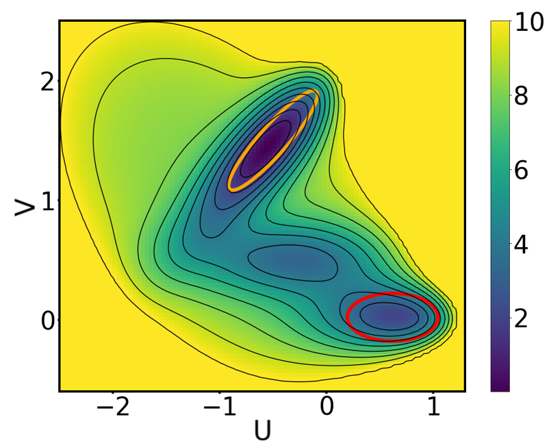
Figure 1: Müller-Brown potential. Orange and red ovals indicate states $A$ and $B$, respectively.

V.1 Comparison of algorithms

A key point of our theoretical development is that NEUS and BAD-NEUS are simple elaborations of WE. This enables us to define a unified walker-based algorithm that we use in practice (Algorithm 4, with the added operations needed for NEUS and BAD-NEUS in Algorithm 5). Splitting and stratification are defined through the rule for switching the index process. The sequence of stopping times $S(\ell)$ is then determined by the index process through (3). The update rule for $J_{t}$ that we employ for all three algorithms is as follows. Let $\{\psi_{k}(x)\}_{k=1,\ldots,n}$ be a set of nonnegative functions. If $\psi_{J_{t}}(X_{t+dt})>0$, then $J_{t+dt}=J_{t}$; otherwise, $\mathbbm{P}[J_{t+dt}=k]=\psi_{k}(X_{t+dt})/\sum_{k}\psi_{k}(X_{t+dt})$. That is, the value of the index process remains the same until the walker leaves the support of $\psi_{J_{t}}$, and then a new index value $k$ is drawn with likelihood proportional to $\psi_{k}(X_{t+dt})$. For the Müller-Brown model, we use

$$\psi_{k}(u,v)=\begin{cases}1&\text{if}\ |v-v_{k}|<\varepsilon_{k}\ \text{and}\ 1<k<n\\ 1&\text{if}\ v-v_{k}<\varepsilon_{k}\ \text{and}\ k=1\\ 1&\text{if}\ v_{k}-v>\varepsilon_{k}\ \text{and}\ k=n\\ 0&\text{otherwise}.\end{cases}$$ (36)

Unless otherwise indicated, we set $n=10$, space the $v_{k}$ uniformly in the interval $[-0.2,1.8]$, and set $\varepsilon_{k}=0.6(v_{k+1}-v_{k})$, so that the regions of support (strata) overlap. This choice prevents walkers in barrier regions from rapidly switching back and forth between index values, limiting the overhead of the algorithms. Unless otherwise indicated, we use 2000 walkers per region and run them until their index processes switch values. Initial configurations for $J_{0}=k$ are generated by uniformly sampling the support of $\psi_{k}$.

For BAD-NEUS, we use a basis set consisting of 10 indicator functions per stratum. The indicator functions are determined by clustering all the samples in a stratum with $k$-means clustering and partitioning it into Voronoi polyhedra based on the cluster means. Unless otherwise indicated, we compute statistics using data from the last $h=3$ iterations and use a lag time of $\tau=10$ time steps.

We measure convergence by computing the root mean square (RMS) difference in $\ln(\tilde{\pi}(x))$ from $-\beta V$, where $\tilde{\pi}(x)$ is an estimate of the steady-state distribution from the normalized histogram of samples. For the histogram, we use a uniform $50\times 50$ grid on the rectangle defined by the minimum and maximum values in the NEUS dataset. Since some grid regions are empty because they correspond to energies too high for NEUS to sample, we only compute errors over bins with $V<7$. We stop each simulation when the RMS difference drops below one. Results are shown in Figure 2. We see that WE requires about 73 times more iterations than NEUS, which in turn requires about 13 times more iterations than BAD-NEUS to reach the convergence criterion.

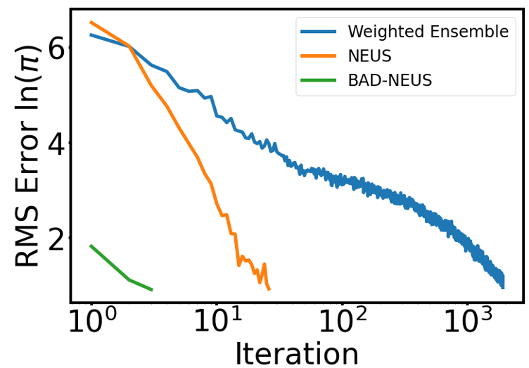
Figure 2: Convergence of the steady-state distribution of the Müller-Brown system for different algorithms as indicated.

V.2 Choice of hyperparameters

Having demonstrated that trajectory stratification outperforms WE for this system, we now examine the effect of key hyperparameters in NEUS and BAD-NEUS.

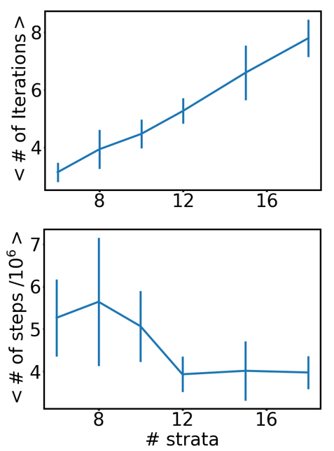
Figure 3: Effect of the number of strata on convergence of BAD-NEUS applied to the Müller-Brown system. The number of iterations required (top) and the total number of time steps (bottom)—a proxy for computational effort—until convergence. The total number of walkers is held fixed. Error bars are the standard deviation over 10 replicate simulations. For these simulations, there are 40,000 walkers total, and the lag time is $\tau=1$ time step.

First, we investigate the effect of the number of strata. To compare simulations that require essentially the same resources, we hold the total number of walkers fixed at 40,000, and we divide the walkers uniformly across the strata. For these simulations, we use a lag time of $\tau=1$ and retain $h=3$ past iterations. In Figure 3 we plot both the number of iterations to reach convergence and the total number of time steps needed for convergence as we vary the number of strata. We see that the number of BAD-NEUS iterations required for convergence increases linearly with the number of strata. However, the lengths of trajectories decrease because the strata are spaced more closely. Due to this interplay, the total effort to achieve convergence decreases until about 12 strata and then levels off. While actual performance will depend on the overhead incurred by stopping and starting the dynamics engine and computing the BAD-NEUS weights, these results indicate that finer stratification is better.

Figure 4: Effect of retaining past iterations on convergence of NEUS (top) and BAD-NEUS (bottom) applied to the Müller-Brown system.

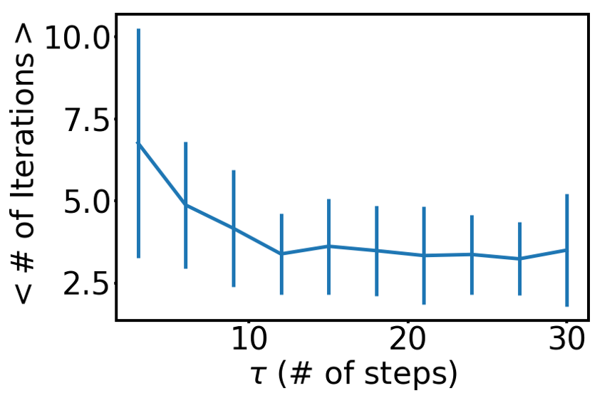
Figure 5: Dependence of convergence on the lag time for BAD-NEUS applied to the Müller-Brown system. Error bars are the standard deviation over 10 replicate simulations.

Next, we examine the dependence of convergence on the number of iterations used to compute statistics, $h$ (other hyperparameters are set to the default values given above). Using data from a larger number of iterations allows for more averaging, but it can also contaminate the statistics with samples obtained before the steady-state distribution has converged. While the trends are clearer for NEUS than BAD-NEUS because the former converges more slowly, Figure 4 indicates that retaining fewer iterations is better for both NEUS and BAD-NEUS. It is therefore important to use enough walkers per iteration that data from past iterations need not be retained. If one has access to a large number of processing elements, and many walkers can be simulated in parallel, this is not a severe restriction. Once convergence is achieved one can begin accumulating data to reduce variance.

Finally, we investigate the impact of the lag time in Figure 5 (other hyperparameters are set to the default values given above). We find that using longer lag times weakly decreases the number of iterations required for convergence.

V.3 Kinetic statistics

A common problem in molecular dynamics is that while equilibrium averages are relatively straightforward to calculate from biased simulations (via, for example, the various methods reviewed in Ref. 32), dynamical averages are much harder. In this section, we use BAD-NEUS to compute dynamical averages efficiently. To do so, we split the ensemble of transition paths based on the last metastable state visited as previously for NEUS [33, 16, 25]. We specifically compute the backward committor, $q_{-}$, which is the probability that the system last visited a reactant state $A$ rather than a product state $B$, and the transition path theory (TPT) rate, defined as the mean number of $A$ to $B$ transitions per unit time divided by the fraction of time spent last in $A$. The former can be obtained without saving additional information once we split the path ensemble. The forward committor, $q_{+}$, which is the probability that the system next visits state $B$ rather than state $A$, can also be obtained from NEUS but requires saving additional information [25]. Here, both of the systems that we consider are microscopically reversible, so we can obtain $q_{+}$ from $q_{+}=1-q_{-}$.

For the Müller-Brown system, we consider the following history dependent stratification. Let $\{\psi_{k}^{A}(x)\}_{k=1,\ldots,n}$ and $\{\psi_{k}^{B}(x)\}_{k=1,\ldots,m}$ be non-negative functions, let $\psi_{k}=\psi_{k}^{A}$ if $k\leq n$; otherwise, let $\psi_{k}=\psi_{k-n}^{B},$ and let $\mathbbm{1}_{A}$ and $\mathbbm{1}_{B}$ be indicator functions on sets $A$ and $B$, respectively. Let $T^{-}_{A\cup B}(t)$ be the time the system sampled at time $t$ was last in $A$ or $B$, so that $\mathbbm{1}_{A}(X_{T^{-}_{A\cup B}(t)})=1-\mathbbm{1}_{B}(X_{T^{-}_{A\cup B}(t)})$ reports whether $A$ rather than $B$ was last visited. Define the index process by the following update rule:

$$\mathbbm{P}[J_{t+dt}=k]=\begin{cases}\psi_{k}(X_{t+dt})\mathbbm{1}_{A}(X_{T^{-}_{A\cup B}(t+dt)})/\sum_{i}\psi_{i}^{A}(X_{t+dt})&k\leq n,\psi_{J_{t}}(X_{t+dt})=0\text{ or }\\ &\quad\quad\quad\mathbbm{1}_{A}(X_{T^{-}_{A\cup B}(t+dt)})\neq\mathbbm{1}_{A}(X_{T^{-}_{A\cup B}(t)})\\ \psi_{k}(X_{t+dt})\mathbbm{1}_{B}(X_{T^{-}_{A\cup B}(t+dt)})/\sum_{i}\psi_{i}^{B}(X_{t+dt})&k>n,\psi_{J_{t}}(X_{t+dt})=0\text{ or }\\ &\quad\quad\quad\mathbbm{1}_{A}(X_{T^{-}_{A\cup B}(t+dt)})\neq\mathbbm{1}_{A}(X_{T^{-}_{A\cup B}(t)})\\ \mathbbm{1}_{\{k\}}(J_{t})&\text{otherwise}\end{cases}$$ (37)

Thus there are $n+m$ total strata, the first $n$ of which contain walkers that last visited $A$, and the remainder of which contain walkers that last visited $B$. The steady-state distribution of walkers which last visited $A$ is proportional to $\pi(x)q_{-}(x)$, and that which last visited $B$ is proportional to $\pi(1-q_{-}(x))$. This ensemble lets us compute dynamical averages. The backward committor projected onto a space of CVs can be computed using

$$q_{-}^{\theta}(s)=\frac{\mathbbm{E}[\mathbbm{1}_{\{0,\ldots,n\}}(J_{t})\mathbbm{1}_{\{ds\}}(\theta(X_{t}))]}{\mathbbm{E}[\mathbbm{1}_{\{ds\}}(\theta(X_{t}))]},$$ (38)

where $\theta$ is a vector with components that are the CVs and $ds$ is a bin in the space. The TPT rate constant is defined as

$$k_{AB}=\frac{\operatorname{\mathbbm{E}}_{\pi}[q_{-}(x)\mathbbm{1}_{B^{c}}(x)\mathcal{T}_{1}\mathbbm{1}_{B}(x)]}{\operatorname{\mathbbm{E}}_{\pi}[q_{-}(x)]},$$ (39)

where $\mathcal{T}_{t}$ is the operator that describes the evolution of expectations of functions:

$$\mathcal{T}_{t}g(x,j)=E_{X_{0}=x,J_{0}=j}[f(X_{t},J_{t})].$$ (40)

In practice, we compute (39) from (16) by choosing

$$g(X_{0},J_{0}...,X_{t},J_{t})=\\ \mathbbm{1}_{B^{c}}(X_{0})\mathbbm{1}_{B}(X_{1})\mathbbm{1}_{\{0,\ldots,n\}}(J_{0})$$ (41)

for the numerator and

$$g(X_{0},J_{0}...,X_{t},J_{t})=\mathbbm{1}_{\{0,\ldots,n\}}(J_{0})$$ (42)

for the denominator. This corresponds to the steady-state flux into $B$ from trajectories that originated in $A$.

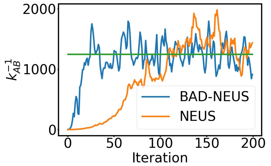
Figure 6: Convergence of the TPT inverse rate estimate for the Müller-Brown system. The green line is the grid-based reference obtained from 44. For these simulations, there are 2000 walkers per stratum, $h=4$ iterations are retained, and the lag time is $\tau=10$ time steps.

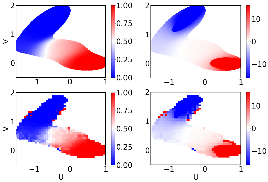
Figure 7: Illustration of the backward committor computed from BAD-NEUS. (top) Reference. (bottom) BAD-NEUS results. (left) Backward committor. (right) $\ln(q_{-}/(1-q_{-}))$, which emphasizes states near $A$ and $B$. These results are obtained from the same simulations as Fig. 6.

For the Müller-Brown system, we define states $A$ and $B$ as

$$A=\{y,v:6.5(u+0.5)^{2}-11(u+0.5)(v-1.5)+6.5(u-1.5)^{2}<0.3\}$$ (43)

$$B=\{u,v:(u-0.6)^{2}+0.5(v-0.02)^{2}<0.2\}.$$

We use a similar index process construction as for the equilibrium calculations, except there are 10 $v_{k}$ that are evenly spaced in the interval $[0,1.6]$ for $\psi_{k}^{A}$ and 10 $v_{k}$ that are evenly spaced in the interval $[-0.3,0.8]$ for $\psi_{k}^{B}$, for a total of 20 strata. We use different definitions for $\psi_{k}^{A}$ and $\psi_{k}^{B}$ because, for walkers originating from state $A$ ($B$), a stratum located below (above) state $B$ ($A$) is unlikely be populated. Both NEUS and BAD-NEUS use 2000 walkers per stratum, and we compute statistics using data from the last $h=3$ iterations. For BAD-NEUS, we use a basis set consisting of 10 indicator functions per stratum, again based on $k$-means clustering; we use a lag time of $\tau=1$.

To compute reference values for these kinetic statistics, we use the grid-based approximation to the generator in Ref. 27, with the same grid parameters. Since the dynamics are microscopically reversible, we obtain the backward committor by solving for the forward committor using the approach in Ref. 27, then setting $q_{-}=1-q_{+}$. We solve for the reaction rate using

$$k_{AB}=\frac{2(\vec{\pi q}_{-})^{\top}(P\vec{\mathbbm{1}}_{B})}{(\vec{\pi}^{\top}\vec{q}_{-})(\beta\epsilon_{x})},$$ (44)

where $P$ is the discretized transition matrix defined on the grid, $\epsilon_{x}$ is the grid spacing, and arrows indicate vectors of function values on the grid points ($\vec{\pi q}_{-}$ is a single vector of product values).

Figure 6 shows estimates for the TPT rate. We see that BAD-NEUS converges several fold faster than NEUS. Each BAD-NEUS iteration requires an average of 407 time units of sampling (arising from 2000 walkers in each of 20 strata, with an average time before leaving the stratum of 10.2 time steps). Each iteration is therefore significantly less total computational cost than generating a single $A$ to $B$ transition on average (1200 time units, as evidenced by $k_{AB}^{-1}$) and is amenable to parallelization.

Figure 7 shows the backward committor computed at BAD-NEUS iteration 20 using (38) with the variables of numerical integration as the CVs. We represent the results in two ways: the committor itself and its logit function. The former emphasizes the transition region ($q_{-}\approx 0.5$) while the latter emphasizes values close to states $A$ and $B$ ($q_{-}\approx 0$ and $q_{-}\approx 1$). Both show excellent agreement with the reference.

VI Molecular Test System

As a more challenging test of the method, we estimate the folding rate of the first 39 amino acids of the N-terminal domain of ribosomal protein L9 (NTL9). The native secondary structure of NTL9 is $\beta\beta\alpha\beta\alpha$ sequentially. In the native state, the $\beta$-strands form an anti-parallel $\beta$-sheet, and the $\alpha$-helices pack on either side of it. NTL9(1-39) lacks the C-terminal helix (Fig. 8). We choose this system because it enables direct comparison with an earlier computational study [34] (described further below), which estimated the folding to be on the millisecond timescale, consistent with experimental studies of (full) NTL9 [35, 36] and earlier simulations of NTL9(1-39) [37].

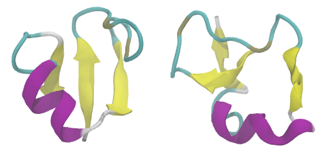
Figure 8: Representative NTL9(1-39) structures drawn from the (left) native and (right) denatured states in the BAD-NEUS simulation. There is residual helical structure in the denatured state in both our simulations and those to which we compare [34].

All molecular dynamics simulations were performed with OpenMM [38]. We compute CVs including backbone RMSDs and fractions of native contacts using MDtraj [39]. To enable direct comparison with Ref. 34, we model NTL9(1-39) using the AMBER FF14SB force field [40] and the Hawkins, Cramer and Truhlar generalized Born implicit solvent model [41, 42]. We use a Langevin thermostat with a time step of 2 fs, a temperature of 300. K, and a friction constant of $\gamma=80$ ps^-1, which corresponds to the high-viscosity case considered in Ref. 34.

We run the molecular dynamics for each walker in intervals of 20 ps and compute the CVs to update the index process at the end of each interval. For BAD-NEUS, after an index process changes values (($S(1)$ in (3)), we run the walker $\tau$ additional molecular dynamics steps to ensure that we have a total of $\tau$ steps beyond $S(1)$. While this procedure allows walkers to run beyond the time that they exit their stratum, it does not bias the results. Since our algorithm only requires us to stop and start the molecular dynamics engine while running unbiased dynamics, we do not need to modify OpenMM in any way.

The stratification is similar to that for the Müller-Brown system. Namely, we set

$$\psi_{k}^{A}(X)=\psi_{k}^{B}(X)=\begin{cases}1&\text{if}\ |Q(X)-Q_{k}|<\varepsilon_{k}\\ 0&\text{otherwise},\end{cases}$$ (45)

where $Q(X)$ is the fraction of native contacts using the definition of Ref. 43. We determine the native contacts from the crystal structure, PDB ID 2HBB[44]. We space 20 $Q_{k}$ values uniformly in the interval $[0.35,0.85]$ and set $\varepsilon_{k}=0.6(Q_{k+1}-Q_{k})$, so that the regions overlap. Thus there are 40 total strata. We define the folded state as full backbone RMSD $<0.28$ nm and $Q>0.85$; the denatured state has full backbone RMSD $>0.80$ nm and $Q<0.35$.

To initialize the simulation, we minimize the energy starting from the PDB structure, draw velocities from a Maxwell-Boltzmann distribution for 380 K, and simulate for 80 ns at that temperature; this denatures the protein (Fig. 8). We sample 4000 frames in each of the 40 strata from this trajectory and weight them uniformly; this set forms our starting walkers, $\{X^{i}_{0},J^{i}_{0},1/N\}_{i=1}^{N}$, where $N=40$. We use a lag time of 10 ps, and we retain a history of $h=4$ iterations. The initialization pipeline, integrator settings, and stratification choice are the same between NEUS and BAD-NEUS. The hyperparameter choices are summarized in Table 1.

Table 1: Hyperparameter choices used for NTL9(1-39) simulations

Hyperparameter	Kinetic statistics
Stratification CV	$Q$ and $\mathbbm{1}_{A}(T^{-}_{A\cup B}(t))$
Stopping rule	Stratum exit
Walkers per stratum	4000
Number of strata	40
Number of iterations retained, $h$	4
Type of basis set	$k$-means indicator
Number of basis functions per stratum	10
Lag time, $\tau$	10 ps

To construct the basis set for BAD-NEUS, we define the following seven CVs: (1) the fraction of native contacts, (2) the full backbone RMSD, (3-5) the backbone RMSD for each of the three $\beta$-strands taken individually (residues 1-4, 17-20, and 36-38), (6) the backbone RMSD for the $\alpha$-helix (residues 22-29), and (7) the backbone RMSD for the three $\beta$-strands together. Our basis set consists of 10 indicator functions on each stratum constructed by $k$-means clustering on the seven-dimensional CV space. At each iteration (i.e., one pass through the outer loop in Algorithm 4), we determine the basis functions for stratum $j$ by taking the associated cluster centers from the prior iteration and refining them with 10 iterations of Lloyd’s algorithm [45] using all the samples with index process $J_{t}^{i}=j$ from the last $h$ iterations.

Here we focus on the convergence of the folding rate; a detailed analysis of the NTL9 folding mechanism (with and without the C-terminal helix) based on potentials of mean force and committors will be presented elsewhere (see also Ref. 46). As mentioned above, we compare our results to those of Ref. 34, which estimates rates using haMSMs applied to data from WE (haMSM-WE). As discussed in the Introduction, BAD-NEUS goes beyond haMSM-WE by using the basis set (Markov model) to accelerate the convergence of the sampling rather than just the rate estimates.

Figure 10 shows the inverse rate constant obtained from BAD-NEUS and haMSM-WE [34]. The average inverse rate over the final 15 iterations of BAD NEUS is 4.74 ms, with a standard deviation of 0.99 ms, while the authors of Ref. 34 used a Bayesian bootstrapping approach to estimate a confidence interval of 0.17–1.9 ms, which they state is likely an underestimate of the true 95 percent confidence interval owing to the limited number of independent samples used in the analysis. Given that we have only a single BAD NEUS run, the standard deviation of the final 15 (highly correlated) inverse rate estimates is also likely a significant underestimate of our statistical error. We thus view the results in Figure 10 as in agreement.

We examine the weights in more detail in Figure 9. The increase in the inverse rate around iteration 35 in Figure 10 (and concommitant decrease in below 5 in Figure 9(bottom)) corresponds to a shift in the weights of strata with indices close to 25 (compare iterations 30 and 45 in Figure 9(top)). These strata contain walkers that are nearly denatured from trajectories that last visited the native state, and the shift in weights in that region stabilizes the denatured state relative to the native state.

Both BAD-NEUS and haMSM-WE required significantly less aggregate simulation to compute the rate constant (an average) than the millisecond timescale of a single folding event. The haMSM-WE calculation used an aggregate simulation time of 252 $\mu$s, while we use an average of 4 $\mu$s per iteration, for a total of about 204 $\mu$s. The speedup is actually more than it appears because the haMSM-WE calculation is for the forward (folding) direction only; computing potentials of mean force and committors would also require the corresponding calculation for the backward (unfolding) direction. By contrast, the BAD-NEUS simulation provides these statistics in its present form.

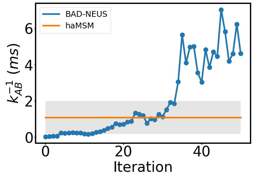
Figure 9: Comparison of inverse rates for NTL9(1-39) folding from NEUS, BAD-NEUS and haMSM-WE. The haMSM-WE results are from Ref. 34 The shaded area shows the Bayesian $95\%$ credible interval reported in that publication.

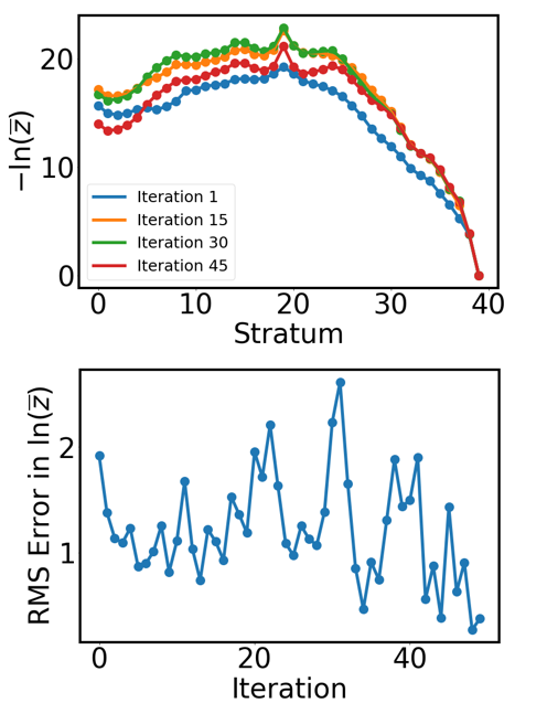
Figure 10: (top) BAD NEUS bin weights for the NTL9(1-39) system. Strata with indices less than 20 correspond to the folding direction (trajectories last in the denatured state), and strat with indices greater than or equal to 20 correspond to the unfolding direction (trajectories last in the native state). (bottom) Deviation of weights ($\ln(\overline{z})$) from those in the last iteration.

VII Conclusions

Trajectory stratification methods enable enhanced sampling for estimating both thermodynamic (equilibrium) and kinetic (nonequilibrium) statistics. Here, we introduced a new trajectory stratification method, BAD-NEUS, which converges faster than existing ones. We show that our method is a natural generalization of WE as originally formulated [1] but that, without modification, WE converges no faster than unbiased dynamics. The key modification that we introduce is the insertion of an approximation to the steady-state distribution before the resampling step. This approximation algorithm is designed so that it preserves the steady-state distribution of the dynamics, and therefore does not introduce systematic errors into the algorithm in the large data limit.

In the present study, we use a simple basis expansion to model the steady-state distribution, but our strategy is general, and alternatives are also possible. One can use neural networks to learn the steady-state distribution and/or the basis functions [26, 27], and one can incorporate memory into a basis expansion [47]. These alternatives, which can be used separately or together, alleviate the need to identify basis sets that describe the dynamics well and, in the case of memory, may reduce the sampling required. We thus expect our method to be a significant be step toward accurate estimates of rates for protein folding and similarly complex molecular conformational changes.

Appendix A Derivation of (16)

Here we derive (16) by modifying the proof from Ref. 48. Let $Z_{t}$ be a Markov process, $\mathcal{T}_{t}$ be operator defined in (40), and $S_{n}=\sum_{t=0}^{n-1}g(Z_{t})$ be the partial sum of a function $g$. Let $\omega(z)$ satisfy the linear problem

$$(\mathcal{T}_{1}-\mathcal{I})\omega(z)=-(g(z)-\mathbbm{E}_{\pi}[g(z)])$$ (46)

subject to the constraint $\mathbbm{E}_{\pi}[\omega]=0$.

Consider the process:

$$U_{n}=S_{n}-\mathbbm{E}_{\pi}[g]n+\omega(Z_{n})$$ (47)

Then $U_{t}$ is a martingale with respect to $Z_{0},...,Z_{t}$. To see this, we compute:

$$\mathbbm{E}[U_{t+1}-U_{t}|Z_{0},...Z_{t}] =\mathbbm{E}[S_{t+1}-\operatorname{\mathbbm{E}}_{\pi}[g](t+1)+\omega(Z_{t+1})-\left(S_{t}-\mathbbm{E}_{\pi}[g]t+\omega(Z_{t})\right)|Z_{0},...Z_{t}]$$

$$=\mathbbm{E}[g(Z_{t})-\operatorname{\mathbbm{E}}_{\pi}[g]+\omega(Z_{t+1})-\omega(Z_{t})|Z_{0},...Z_{t}]$$

$$=g(Z_{t})-\operatorname{\mathbbm{E}}_{\pi}[g]+\mathbbm{E}[\omega(Z_{t+1})-\omega(Z_{t})|Z_{0},...Z_{t}]$$

$$=g(Z_{t})-\operatorname{\mathbbm{E}}_{\pi}[g]+(\mathcal{T}_{1}-\mathcal{I})\omega(Z_{t})$$

$$=g(Z_{t})-\operatorname{\mathbbm{E}}_{\pi}[g]-g(Z_{t})+\mathbbm{E}_{\pi}[g]$$

$$=0.$$ (48)

We refer the reader to Ref. 48 for a more technical discussion and conditions under which the relevant expectations are bounded such that we may apply the optional stopping theorem. Then, for any stopping time $T$ with $\operatorname{\mathbbm{E}}[T]<\infty$,

$$0=\operatorname{\mathbbm{E}}[U_{T}-U_{0}]=\operatorname{\mathbbm{E}}[S_{T}]-\operatorname{\mathbbm{E}}_{\pi}[g]\operatorname{\mathbbm{E}}[T]+\operatorname{\mathbbm{E}}[\omega(Z_{T})]-\operatorname{\mathbbm{E}}[\omega(Z_{0})],$$ (49)

which yields the result:

$$\frac{\operatorname{\mathbbm{E}}[\sum_{t=0}^{T-1}g(Z_{t})]}{\operatorname{\mathbbm{E}}[T]}=\operatorname{\mathbbm{E}}_{\pi}[g]+\frac{\operatorname{\mathbbm{E}}[\omega(Z_{0})]-\operatorname{\mathbbm{E}}[\omega(Z_{T})]}{\operatorname{\mathbbm{E}}[T]}.$$ (50)

Now take $Z_{t}=(X_{t},J_{t},...,X_{t+\tau},J_{t+\tau})$ and take the stopping time to be $S(1)$. In the case where $X_{0},J_{0}$ is distributed according to the steady state flux distribution $\overline{\pi}(dx,k),$ (9) implies that $(X_{T},J_{T})\sim\overline{\pi}(dx,k)$, and hence the distribution of $Z_{0}$ and $Z_{T}$ are the same, and so the residual term in (50) is zero. In this case, we note that the distribution of $(X_{0},J_{0})$ is given by:

$$\pi(dx) =\mathbbm{P}[X_{0}\in dx]$$ (51)

$$=\sum_{k}\mathbbm{P}[X_{0}\in dx\mid J_{0}=k]\mathbbm{P}[J_{0}=k]$$ (52)

$$=\sum_{k}\overline{z}^{k}\overline{\pi}(dx|k).$$ (53)

The joint distribution for $(X,J)$ is $\overline{\pi}(dx,k)=\overline{z}^{k}\overline{\pi}(dx|k)$. Therefore,

$$\mathbbm{E}\left[\sum_{t=0}^{S(1)-1}g(X_{t},J_{t},...,X_{t+\tau},J_{t+\tau})\right]=\sum_{k}\overline{z}^{k}\int\overline{\pi}(dx|k)\mathbbm{E}_{X_{0}=x,J_{0}=k}\left[\sum_{t=0}^{S(1)-1}g(X_{t},J_{t},...,X_{t+\tau},J_{t+\tau})\right]$$ (54)

and

$$\mathbbm{E}[S(1)]=\sum_{k}\overline{z}^{k}\int\overline{\pi}(dx|k)\mathbbm{E}_{X_{0}=x,J_{0}=k}[S(1)].$$ (55)

Substituting these into (50) and remembering that the residual term is zero yields (16).

References

- [1] G. A. Huber and S. Kim. Weighted-ensemble Brownian dynamics simulations for protein association reactions. Biophysical Journal, 70(1):97–110, January 1996.
- [2] Rosalind J. Allen, Chantal Valeriani, and Pieter Rein ten Wolde. Forward flux sampling for rare event simulations. Journal of Physics: Condensed Matter, 21(46):463102, October 2009.
- [3] Aryeh Warmflash, Prabhakar Bhimalapuram, and Aaron R. Dinner. Umbrella sampling for nonequilibrium processes. Journal of Chemical Physics, 127(15):154112, October 2007.
- [4] Alex Dickson and Aaron R Dinner. Enhanced sampling of nonequilibrium steady states. Annual review of physical chemistry, 61:441–459, 2010.
- [5] Nicholas Guttenberg, Aaron R Dinner, and Jonathan Weare. Steered transition path sampling. The Journal of Chemical Physics, 136(23), 2012.
- [6] Juan M. Bello-Rivas and Ron Elber. Exact milestoning. Journal of Chemical Physics, 142(9):094102, March 2015.
- [7] Daniel M Zuckerman and Lillian T Chong. Weighted ensemble simulation: review of methodology, applications, and software. Annual review of biophysics, 46:43–57, 2017.
- [8] John D. Russo, She Zhang, Jeremy M. G. Leung, Anthony T. Bogetti, Jeff P. Thompson, Alex J. DeGrave, Paul A. Torrillo, A. J. Pratt, Kim F. Wong, Junchao Xia, Jeremy Copperman, Joshua L. Adelman, Matthew C. Zwier, David N. LeBard, Daniel M. Zuckerman, and Lillian T. Chong. WESTPA 2.0: High-Performance Upgrades for Weighted Ensemble Simulations and Analysis of Longer-Timescale Applications. Journal of Chemical Theory and Computation, 18(2):638–649, February 2022. Publisher: American Chemical Society.
- [9] D. Aristoff, J. Copperman, G. Simpson, R. J. Webber, and D. M. Zuckerman. Weighted ensemble: Recent mathematical developments. Journal of Chemical Physics, 158(1):014108, January 2023.
- [10] Surl-Hee Ahn, Anupam A. Ojha, Rommie E. Amaro, and J. Andrew McCammon. Gaussian-Accelerated Molecular Dynamics with the Weighted Ensemble Method: A Hybrid Method Improves Thermodynamic and Kinetic Sampling. Journal of Chemical Theory and Computation, 17(12):7938–7951, December 2021. Publisher: American Chemical Society.
- [11] Anupam Anand Ojha, Saumya Thakur, Surl-Hee Ahn, and Rommie E. Amaro. DeepWEST: Deep Learning of Kinetic Models with the Weighted Ensemble Simulation Toolkit for Enhanced Sampling. Journal of Chemical Theory and Computation, 19(4):1342–1359, February 2023. Publisher: American Chemical Society.
- [12] Jeremy Copperman and Daniel M. Zuckerman. Accelerated Estimation of Long-Timescale Kinetics from Weighted Ensemble Simulation via Non-Markovian “Microbin” Analysis. Journal of Chemical Theory and Computation, 16(11):6763–6775, November 2020. Publisher: American Chemical Society.
- [13] Alex J. DeGrave, Anthony T. Bogetti, and Lillian T. Chong. The RED scheme: Rate-constant estimation from pre-steady state weighted ensemble simulations. The Journal of Chemical Physics, 154(11):114111, March 2021.
- [14] Ernesto Suárez, Steven Lettieri, Metthew C Zwier, Sundar Raman Subramanian, Lillian T Chong, and Daniel M Zuckerman. Simultaneous computation of dynamical and equilibrium information using a weighted ensemble of trajectories. Biophysical Journal, 106(2):406a, 2014.
- [15] Alex Dickson, Aryeh Warmflash, and Aaron R Dinner. Nonequilibrium umbrella sampling in spaces of many order parameters. Journal of chemical physics, 130(7), 2009.
- [16] Alex Dickson, Aryeh Warmflash, and Aaron R Dinner. Separating forward and backward pathways in nonequilibrium umbrella sampling. Journal of chemical physics, 131(15), 2009.
- [17] Alex Dickson, Mark Maienschein-Cline, Allison Tovo-Dwyer, Jeff R Hammond, and Aaron R Dinner. Flow-dependent unfolding and refolding of an rna by nonequilibrium umbrella sampling. Journal of Chemical Theory and Computation, 7(9):2710–2720, 2011.
- [18] Aaron R. Dinner, Jonathan C. Mattingly, Jeremy O. B. Tempkin, Brian Van Koten, and Jonathan Weare. Trajectory Stratification of Stochastic Dynamics. SIAM Review, 60(4):909–938, January 2018. Publisher: Society for Industrial and Applied Mathematics.
- [19] Divesh Bhatt, Bin W. Zhang, and Daniel M. Zuckerman. Steady-state simulations using weighted ensemble path sampling. Journal of Chemical Physics, 133(1):014110, July 2010.
- [20] Gabriel Earle and Jonathan Mattingly. Convergence of Stratified MCMC Sampling of Non-Reversible Dynamics, February 2022. arXiv:2111.05838 [math].
- [21] Gabriel Earle and Brian Van Koten. Aggregation methods for computing steady states in statistical physics. Multiscale Modeling & Simulation, 21(3):1170–1209, 2023.
- [22] Erik H. Thiede, Dimitrios Giannakis, Aaron R. Dinner, and Jonathan Weare. Galerkin Approximation of Dynamical Quantities using Trajectory Data. Journal of Chemical Physics, 150(24):244111, 2019.
- [23] John Strahan, Adam Antoszewski, Chatipat Lorpaiboon, Bodhi P. Vani, Jonathan Weare, and Aaron R. Dinner. Long-Time-Scale Predictions from Short-Trajectory Data: A Benchmark Analysis of the Trp-Cage Miniprotein. Journal of Chemical Theory and Computation, 17(5):2948–2963, 2021.
- [24] Justin Finkel, Robert J. Webber, Dorian S. Abbot, Edwin P. Gerber, and Jonathan Weare. Learning forecasts of rare stratospheric transitions from short simulations. Monthly Weather Review, 149(11):3647–3669, 2021.
- [25] Bodhi P. Vani, Jonathan Weare, and Aaron R. Dinner. Computing transition path theory quantities with trajectory stratification. Journal of Chemical Physics, 157(3):034106, July 2022.
- [26] Junfeng Wen, Bo Dai, Lihong Li, and Dale Schuurmans. Batch stationary distribution estimation. In Proceedings of the 37th International Conference on Machine Learning, ICML’20, pages 10203–10213. JMLR.org, 2020.
- [27] John Strahan, Spencer C. Guo, Chatipat Lorpaiboon, Aaron R. Dinner, and Jonathan Weare. Inexact iterative numerical linear algebra for neural network-based spectral estimation and rare-event prediction. Journal of Chemical Physics, 2023.
- [28] Randal Douc, Olivier Cappé, and Eric Moulines. Comparison of Resampling Schemes for Particle Filtering. ISSN: 1845-5921, pages 64–69, 2005.
- [29] John Strahan, Justin Finkel, Aaron R. Dinner, and Jonathan Weare. Predicting rare events using neural networks and short-trajectory data, March 2023. arXiv:2208.01717 [physics].
- [30] Klaus Müller and Leo D. Brown. Location of saddle points and minimum energy paths by a constrained simplex optimization procedure. Theoretica chimica acta, 53(1):75–93, 1979.
- [31] Benedict Leimkuhler and Charles Matthews. Rational construction of stochastic numerical methods for molecular sampling. Applied Mathematics Research eXpress, 2013(1):34–56, 2013.
- [32] Jérôme Hénin, Tony Lelièvre, Michael Shirts, Omar Valsson, and Lucie Delemotte. Enhanced sampling methods for molecular dynamics simulations [article v1. 0]. Living Journal of Computational Molecular Science, 4(1):1583–1583, 2022.
- [33] Eric Vanden-Eijnden and Maddalena Venturoli. Exact rate calculations by trajectory parallelization and tilting. The Journal of chemical physics, 131(4), 2009.
- [34] Upendra Adhikari, Barmak Mostofian, Jeremy Copperman, Sundar Raman Subramanian, Andrew A. Petersen, and Daniel M. Zuckerman. Computational Estimation of Microsecond to Second Atomistic Folding Times. Journal of the American Chemical Society, 141(16):6519–6526, April 2019. Publisher: American Chemical Society.
- [35] Donna L Luisi, Brian Kuhlman, Kostandinos Sideras, Philip A Evans, and Daniel P Raleigh. Effects of varying the local propensity to form secondary structure on the stability and folding kinetics of a rapid folding mixed protein: characterization of a truncation mutant of the N-terminal domain of the ribosomal protein L911Edited by P. E. Wright. Journal of Molecular Biology, 289(1):167–174, May 1999.
- [36] Satoshi Sato, Jae-Hyun Cho, Ivan Peran, Rengin G. Soydaner-Azeloglu, and Daniel P. Raleigh. The N-Terminal Domain of Ribosomal Protein L9 Folds via a Diffuse and Delocalized Transition State. Biophysical Journal, 112(9):1797–1806, May 2017.
- [37] Vincent A Voelz, Gregory R Bowman, Kyle Beauchamp, and Vijay S Pande. Molecular simulation of ab initio protein folding for a millisecond folder ntl9 (1- 39). Journal of the American Chemical Society, 132(5):1526–1528, 2010.
- [38] Peter Eastman, Jason Swails, John D. Chodera, Robert T. McGibbon, Yutong Zhao, Kyle A. Beauchamp, Lee-Ping Wang, Andrew C. Simmonett, Matthew P. Harrigan, Chaya D. Stern, Rafal P. Wiewiora, Bernard R. Brooks, and Vijay S. Pande. OpenMM 7: Rapid development of high performance algorithms for molecular dynamics. PLOS Computational Biology, 13(7):e1005659, July 2017. Publisher: Public Library of Science.
- [39] Robert T. McGibbon, Kyle A. Beauchamp, Matthew P. Harrigan, Christoph Klein, Jason M. Swails, Carlos X. Hernández, Christian R. Schwantes, Lee-Ping Wang, Thomas J. Lane, and Vijay S. Pande. Mdtraj: A modern open library for the analysis of molecular dynamics trajectories. Biophysical Journal, 109(8):1528 – 1532, 2015.
- [40] James A. Maier, Carmenza Martinez, Koushik Kasavajhala, Lauren Wickstrom, Kevin E. Hauser, and Carlos Simmerling. ff14SB: Improving the Accuracy of Protein Side Chain and Backbone Parameters from ff99SB. Journal of Chemical Theory and Computation, 11(8):3696–3713, August 2015. Publisher: American Chemical Society.
- [41] Gregory D. Hawkins, Christopher J. Cramer, and Donald G. Truhlar. Parametrized Models of Aqueous Free Energies of Solvation Based on Pairwise Descreening of Solute Atomic Charges from a Dielectric Medium. Journal of Physical Chemistry, 100(51):19824–19839, January 1996. Publisher: American Chemical Society.
- [42] Gregory D. Hawkins, Christopher J. Cramer, and Donald G. Truhlar. Pairwise solute descreening of solute charges from a dielectric medium. Chemical Physics Letters, 246(1):122–129, November 1995.
- [43] Robert B. Best, Gerhard Hummer, and William A. Eaton. Native contacts determine protein folding mechanisms in atomistic simulations. Proceedings of the National Academy of Sciences, 110(44):17874–17879, October 2013. Publisher: Proceedings of the National Academy of Sciences.
- [44] Jae-Hyun Cho, Wenli Meng, Satoshi Sato, Eun Young Kim, Hermann Schindelin, and Daniel P. Raleigh. Energetically significant networks of coupled interactions within an unfolded protein. Proceedings of the National Academy of Sciences, 111(33):12079–12084, August 2014. Publisher: Proceedings of the National Academy of Sciences.
- [45] S. Lloyd. Least squares quantization in PCM. IEEE Transactions on Information Theory, 28(2):129–137, March 1982. Conference Name: IEEE Transactions on Information Theory.
- [46] John Champlin Strahan. Short trajectory methods for rare event analysis and sampling. 2024.
- [47] Chatipat Lorpaiboon, Spencer C Guo, John Strahan, Jonathan Weare, and Aaron R Dinner. Accurate estimates of dynamical statistics using memory. The Journal of Chemical Physics, 160(8), 2024.
- [48] George V. Moustakides. Extension of Wald’s First Lemma to Markov Processes. Journal of Applied Probability, 36(1):48–59, 1999. Publisher: Applied Probability Trust.