Inverse Modeling of Bubble Size Dynamics for Interphase Mass Transfer and Gas Holdup in CO2 Bubble Column Reactors

Abstract

The use of microbial gas fermentation for transforming captured CO2 into sustainable fuels and chemicals has been identified as a promising decarbonization pathway. To accelerate the scale-up of gaseous CO2 fermentation reactors, computational models need to predict gas-to-liquid mass transfer which requires capturing the bubble size dynamics, i.e. bubble breakup and coalescence. In this work, an inverse modeling approach is used to calibrate the breakup and coalescence closure models, that are used in the Multiple-Size-Group (MUSIG) population balance modeling (PBM). The calibration aims at replicating experimental results obtained in a CO2-air-water-coflowing bubble column reactor. Bayesian inference is used to account for noise in the experimental dataset and bias in the simulation results. The estimated simulation bias also allows identifying the best-performing closure models irrespective of the model parameters used. The calibration results suggest that the breakage rate is underestimated by one order of magnitude in two different breakup modeling approaches.

1 Introduction

1.1 Motivation

In order to control global warming to levels lower than 2^∘C, CO2 emissions need to be rapidly reduced (by 37% in 2035 compared to 2019 emissions) [1]. To this end, demand reduction or decarbonization of carbon-heavy industrial sectors such as chemical manufacturing and aviation [2] is urgently needed. For specific industrial sectors such as aviation, there remain significant challenges to electrification [3], and recent policies have instead incentivized the production of sustainable aviation fuels (SAF) [4].

Given the widespread availability of gaseous CO2 through point sources and direct air capture, a promising pathway towards SAF production is to use CO2 as a carbon feedstock, instead of oil-based products, and several CO2-based SAF production methods have been developed so far [5]. In particular, microbial action to produce valuable SAF intermediates from CO2/syngas or CO2/green-H2 mixtures is increasingly pursued [6], building upon successful microbial genetic engineering strategies developments [7]. Once the appropriate microbial strain is optimized in the laboratory, fuel production relies on operating a gas fermentation reactor where gaseous CO2 is injected into a liquid medium, where microbial bioreactions occur. The rate at which gaseous species transfer into the liquid phase, i.e. the interphase mass transfer, is a significant contributor towards the overall yield of the system.

The interphase mass transfer itself mainly depends on the Henry saturation concentration that varies directly with pressure [8], the interphase slip velocity, and the size of the gas bubbles that determine the overall interphasial area [9]. Computational fluid dynamics (CFD) can facilitate the optimization and scale-up of gas fermentation reactors, and several methods have been proposed to account for variable bubble size. In particular, methods that use a population balance modeling (PBM) approach have been often used for multiphase flows [10, 11, 12]. In the context of bubbly flows, PBM requires closure modeling to represent how bubbles coalesce and breakup. The focus of this work is to improve coalescence and breakup modeling with a specific focus on interphase mass transfer of CO2.

1.2 Bubble size dynamics model calibration

Throughout the past decades, the choice of the coalescence and breakup models has been observed to significantly affect the numerical predictions for liquid-liquid dispersion [13] and gas-liquid dispersion [14, 15]. The effect of the coalescence and breakup models was observed on bubble size distribution [14, 15] and the Sauter mean bubble diameter [14] or droplet diameter [13]. Those observations have led to conclusions that an ensemble of models should be used [15] or that the models need to be calibrated before being used [14, 16, 17, 18].

Several breakup and coalescence model calibration approaches have been undertaken in the past, mostly for liquid-liquid systems [19, 20, 21, 22, 23, 24], but were also extended to gas-liquid systems [16, 17] which are of interest here. Those various efforts have focused on calibrating models in different regimes or against different datasets, and have found different sets of optimal model parameters which can vary by orders of magnitude [21]. This observation highlights the importance of calibrating bubble size model dynamics against targeted experiments [18, 16, 17], and also suggests that parameter calibration is a challenging task.

The first difficulty highlighted by Maluta et al. [25] during a deterministic calibration process is that the calibrated parameters might compensate for numerical errors rather than address modeling deficiencies. This conclusion was drawn based on the observation that pairing calibrated models with fine discretization resulted in higher errors compared to adopting a coarse discretization. The second difficulty identified is that there could exist multiple optimal parameter sets that can explain the same experimental observations [26]. Therefore, the solution of the calibration procedure should be probabilistic rather than deterministic to capture the ensemble of model parameters that explains experimental observations [27]. The last difficulty relates to the appropriate choice of experimental datasets: depending on the experimental dataset used for calibration, different parameters can be identified [27]. As a side note, the issues in bubble size dynamics calibration tasks have led to the development of models that do not contain adjustable parameters [28].

To address the first difficulty, appropriate mesh convergence studies are needed [25]. To address the second difficulty, a probabilistic calibration is needed. Currently, most breakup and coalescence model calibration tasks reported, provide deterministic optimized model parameters [20, 19, 21, 22, 16, 18]. Only a handful of studies analyze the uncertainty in the calibrated model parameters, by using a local sensitivity analysis on the optimal parameter set [23, 24]. The advantage of such methods is that they are efficient in terms of the number of forward simulations - i.e. numerical simulations that predict experimental observations for a given parameter set -, but do not necessarily describe the entire distribution of parameter values. Bayesian inference methods have been devised to accurately characterize the parameters’ distributions, but tend to require a large number of forward simulations [29, 30, 31]. Bayesian inference can be efficiently used when the experimental observations can be simulated with fast physics models [32, 33, 34], or fast surrogate models [35, 36]. To address the third difficulty, combining multiple experimental datasets in the calibration procedure is necessary. When calibrating coalescence and breakup models, experimental datasets are usually combined by minimizing an error fit metric averaged across all the experimental data [22, 27]. However, experimental data may be subject to different levels of noise, and experimental datasets should not be equally weighted in the parameter fitting procedure. Including experimental noise in the calibration procedure is however straightforward using a Bayesian calibration approach [32].

The novel contributions of this work are

• Coalescence and breakup models are calibrated against experimental data of a coflowing bubble column reactor using CO2 in the gas phase. Compared to previous work, the models are calibrated against gas holdup and interphase mass transfer, which are critical parameters for gas fermentation applications.

• A Bayesian inference approach is used to calibrate efficiency factors for coalescence and breakup rates, thereby appropriately estimating confidence intervals on the efficiency factors. The Bayesian inference procedure is made tractable by constructing a data-based surrogate model.

• Four experimental datasets are combined by taking into account experimental uncertainties. We show how uncertainties can be constructed including bias between experiments and numerical simulations. This can also be used to choose the best models irrespective of the parameter calibration task.

In Sec. 2 the numerical modeling approach is described. In Sec. 3, the performance of the non-calibrated models are compared to the experimental dataset of interest [37]. The model calibration problem and the calibration results are shown in Sec. 4. Conclusions are provided in Sec. 5.

2 Numerical method

2.1 Multiphase model

The numerical simulations are conducted with a multiphase solver implemented in OpenFOAM [38] that has been extensively used and validated in the past [39, 40]. The multiphase model is implemented via the Euler-Euler method where gas and liquid are treated as continuous interpenetrating phases. Gas and liquid volume fractions are transported according to

$$\frac{\partial(\alpha_{j}\rho_{j})}{\partial t}+\nabla\cdot(\alpha_{j}\rho_{j}u_{j})=0,$$ (1)

where $j$ is the phase index (gas or liquid), $\alpha_{j}$ is the volume fraction of the phase $j$, $\rho_{j}$ is the density of phase $j$, $u_{j}$ is the velocity vector of phase $j$. To model the relative motion of each phase, a phase-momentum transport equation is solved, which takes the form

$$\frac{\partial(\alpha_{j}\rho_{j}u_{j})}{\partial t}+\nabla\cdot(\alpha_{j}\rho_{j}u_{j}u_{j})=\nabla\cdot(\alpha_{j}\overline{\tau})-\alpha_{j}\nabla p+\alpha_{j}\rho_{j}g+\sum_{k\neq j}D_{kj}+M^{m}_{j}+F_{j},$$ (2)

where $\overline{\tau}$ is the stress tensor which includes Reynolds stress and viscous (molecular and turbulent) stress (including turbulent viscosity) for the phase $j$, $D_{kj}$ is the drag force exerted by phase $k$ on phase $j$, and $F_{j}$ contains interfacial forces acting on phase $j$. Coupling between phase volume fraction and momentum needs to be enforced, including across phases, where drag forces depend on the relative velocities of each phase. In addition, momentum can be added to the system due to mass transfer; mass entering/leaving a specific phase. The term $M^{m}_{j}$ accounts for the added momentum:

$$M^{m}_{j}=\dot{m}_{j,in}u_{k}-\dot{m}_{j,out}u_{j}$$ (3)

where $\dot{m}$ is the mass transfer rate from/to phase $j$, $u_{j}$ is the velocity of phase $j$ and $u_{k}$ is the velocity of phase $k$ [40]. A partial elimination method formulated by Passalacqua and Fox [41] is used here to ensure appropriate coupling between the phases. A shared pressure equation is solved once for all the phases to determine pressure while enforcing an aggregate divergence constraint on phase velocity.

An energy equation is solved to account for different inlet phase temperature (see Sec. 3.1). A sensible energy transport equation for phase $j$ is written as:

$$\frac{\partial\rho_{j}\alpha_{j}E_{j}}{\partial t}+\nabla\cdot(\rho_{j}\alpha_{j}u_{j}E_{j})=\nabla\cdot(\alpha_{j}\kappa_{j}\nabla T_{j})+\dot{Q}$$ (4)

where $E_{j}$ is the sensible energy enthalpy of the phase $j$, $T_{j}$ is the temperature of the phase $j$, $\kappa_{j}$ is the effective thermal diffusivity of the phase $j$(including molecular and turbulent contributions) and $\dot{Q_{T}}$ is the heat exchange due to differences in temperature. In particular the last term can be written as:

$$\dot{Q}=h_{jl}(T_{f}-T_{j})$$ (5)

where $h_{jl}$ is the heat transfer coefficient of species $l$ in phase $j$, $T_{j}$ is the temperature of phase $j$ and $T_{f}$ is the temperature at the interface. Heat exchange through the interface is driven by temperature differences between phases. The temperature at the interface changes as a result of a phase change and depends on the latent heat of the species changing phase. The temperature at the interface is computed based on the assumption that the rate of heat transfer must be equal to the latent heat $\lambda_{j}$ at the interface between phases $j$ and $k$

$$h_{jl}(T_{j}-T_{f})+h_{kl}(T_{k}-T_{f})=\dot{m}_{j,in}\lambda_{j}$$ (6)

Using the momentum and phase fraction, species mass fractions are transported as

$$\frac{\partial(\rho_{j}\alpha_{j}Y_{jl})}{\partial t}+\nabla\cdot(\rho_{j}\alpha_{j}Y_{jl}u_{j})=\nabla\cdot(\rho_{j}\alpha_{j}D_{jl}\nabla Y_{jl})+S_{jl}$$ (7)

where $Y_{jl}$ is the $l^{th}$ species mass fraction in phase $j$, $D_{jl}$ is the diffusivity of the $l^{th}$ species in phase $j$ and $S_{jl}$ are source terms due to interphase mass transfer.

The aforementioned conservation equations are closed through models for interphase physics and turbulent stress. The interphase drag force is obtained by using the Grace model [42] and transverse lift from the model by Tomiyama et al. [43]. Wall lubrication forces are computed using the model by Antal et al. [44] and turbulent dispersion uses the model of Burns et al. [45]. Interphase mass transfer of species is modeled using Higbie [46]. Turbulent stress is modeled using $k-\varepsilon$ RANS closure model for the liquid and the gas phases [47]. The wall boundary conditions for $k$ and $\varepsilon$ use generalized wall functions [48].

2.2 Bubble size models

Compared to our previous works [39], the bubble size distribution (BSD) in this work is not assumed to be a $\delta$-distribution (constant bubble size), but is directly modeled using a population balance equation. In separate studies, several authors have noted the effect of BSD on global hydrodynamics of bubble column reactors [49, 50, 51, 52] and on species mass transfer [53] which is the main focus here.

The population balance model uses a method of classes implementation as described by Lehnigk et al. [40] where the bubble size distribution is represented through a discretization of the number density function (NDF). This approach requires discretizing an internal coordinate (here the bubble size coordinate) and the spatial coordinates. The fundamental governing equation of the NDF can be derived through a finite volume analysis [40] and leads to

$$\frac{\partial n_{v}}{\partial t}+\nabla\cdot(un_{v})=h_{v},$$ (8)

where $u$ is the phase velocity, $t$ is time, $n_{v}$ is the number density of bubbles of size $v$ and the source term $h_{v}=B_{\rm b}-B_{\rm d}+C_{\rm b}-C_{\rm d}+D+\dot{N_{v}}$, where $B_{\rm b}$ (resp. $C_{\rm b}$) is the bubble birth contribution from bubble breakup (resp. coalescence), $B_{\rm d}$ (resp. $C_{\rm d}$) is the bubble death contribution from bubble breakup (resp. coalescence), $D$ is the drift term that is due to changes of bubble volume, and $\dot{N_{v}}$ is the bubble nucleation source term. The full expression of $h_{v}$ is available elsewhere (see Eq.2 in Ref. [40]) and only specific modeling choices are described hereafter. The breakup and coalescence source terms depend on closure models for coalescence and breakup frequencies (also referred to as rates or kernels). For instance, the birth by breakup effect of bubbles of volume $v^{\prime}$ to bubbles of volume $v$ ($v<v^{\prime}$) is represented in $h_{v}$ as

$$B_{\rm b}=\int_{v}^{\infty}B_{v^{\prime}}\beta_{v,v^{\prime}}n_{v^{\prime}}dv^{\prime},$$ (9)

where $B_{v^{\prime}}$ is the breakup frequency of bubbles of volume $v^{\prime}$, and $\beta_{v,v^{\prime}}$ is the daughter size distribution that describes how bubbles are redistributed within the internal coordinate (the binned bubble size). Similarly, the birth by coalescence effect of bubbles with volume $v^{\prime}$ and $v-v^{\prime}$ resulting in a bubble of volume $v$ is represented in $h_{v}$ as

$$C_{\rm b}=\frac{1}{2}\int_{0}^{v}n_{v}^{\prime}n_{v-v^{\prime}}C_{v^{\prime},v-v^{\prime}}dv^{\prime},$$ (10)

where $C_{v^{\prime},v-v^{\prime}}$ is the frequency of coalescence for bubbles of size $v^{\prime}$ and $v-v^{\prime}$.

A noteworthy feature of the implementation of Lehnigk et al. [40] is that it includes redistribution schemes that conserve the 0^th and 1^st order moments of the NDF [54, 55]. The coalescence kernel chosen is that of Lehr et al. [56] using a critical coalescence velocity of $0.08$m/s and a maximum packing density of $0.6$. In this model, the coalescence frequency $C_{v^{\prime},v-v^{\prime}}$ depends on turbulent fluctuations, and coalescence occurs if bubbles collide with a velocity greater than the critical velocity aforementioned. Two breakup models are investigated: a global breakup model described in Laakkonen et al. [17] and a binary breakup model described in Lehr et al. [56] which is common in bubble column reactor modeling [57]. In the binary breakup approach, a bubble necessarily breaks up into two daughter bubbles from different size groups (or bins). In the global breakup approach, a bubble may break up into more than two bubbles [17]. The number of “daughter bubbles” is controlled by the daughter size distribution which differs between both models. The breakup rates used in both of these models differ from the default rates implemented in OpenFOAM v9 , unless stated otherwise.

3 Validation of the base model

In this section, the experimental case simulated is described. A base simulation is compared to the experimental results and the effect of numerical errors and modeling errors is discussed.

3.1 Experimental data

Two experimental cases (Exp. 17 and Exp. 19) are investigated here and documented in Deckwer et al. [37]. The system consists of a coflowing bubble column reactor schematically illustrated in Fig. 2 (left). Both cases differ in terms of their superficial gas velocity and inlet gas composition. These cases were chosen given that they were also used in other numerical analyses such as by Hissanaga et al. [58] and by Ngu et al. [59]. In Exp. 17 the inlet gas velocity is $3.42cm/s$ and the inlet gas CO2 mole fraction is $0.673$. In Exp. 19, the inlet gas velocity is $4.63cm/s$ and the inlet gas CO2 mole fraction is $0.478$. The liquid phase is made of pure water at the inlet. Air is assumed to be pure N2 for simplification. The gas phase inlet temperature is set to $273.15$K consistently with Deckwer et al. [37] and the liquid phase (tap water) inlet temperature is assumed to be $287.15$K.

3.2 Numerical details

A hexahedral mesh was used to simulate these experiments using 180 mesh points of size 2.4 cm each in the vertical direction. A “pillow case” meshing (illustrated in Fig. 1) was used in the radial and azimuthal direction with 15 mesh points through the radial direction and 24 points in the azimuthal direction. In total, 64,800 cells were used.

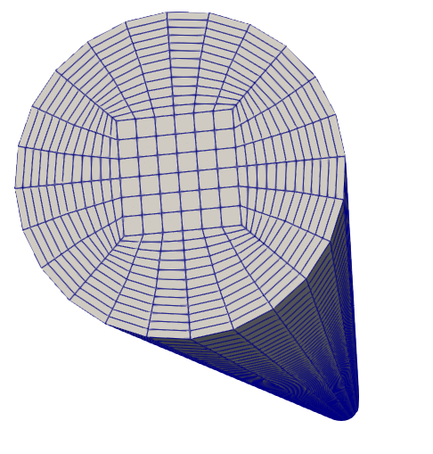
Figure 1: Illustration of the pillow case mesh in the radial and azimuthal directions.

The internal coordinate (bubble diameter) was discretized with 10 classes (bins), uniformly distributed between $1.66~{}\rm{mm}$ and $4.36~{}\rm{mm}$. In separate numerical investigations [59], the bubble size was assumed constant and equal to $2.86~{}\rm{mm}$. Hereafter the global breakup model and binary breakup model as described in Sec. 2 are successively used. Simulations of both Exp. 17 and Exp. 19 use the same numerical discretization. The liquid diffusivity of CO2 was set to $1.4663\times 10^{-9}$ m²/s and the Henry’s constant of CO2 was set to $0.0192$ mg/L/Pa which are the same values used by Ngu et al. [59]. The simulations were run for $400~{}\rm{s}$ which was found to be sufficient to reach steady state in gas holdup and species concentration profiles. Each simulation required about 10 hours of wall clock time on 36 cores of Dual Intel Xeon Gold Skylake 6154 3.0 GHz processors. The timestep is dynamically adjusted based on the maximal Courant number, and was $2~{}\rm{ms}$ on average. Inlet boundary conditions for $k$ and $\varepsilon$ based on freestream turbulence were found to lead to steep wall-normal gradients due to the wall functions used, and could lead to unphysical oscillations in $\alpha_{j}$. The boundary conditions were adjusted to eliminate these oscillations without inducing appreciable differences in the quantities of interest (see B).

Figure 2 (right) shows the CO2 mass fraction contour in the gas phase and the liquid phase for Exp. 17 which illustrates how the interphase mass transfer occurs in the coflowing bubble column. The gas phase is gradually depleted of CO2 with height (z in Fig. 2) while the liquid phase CO2 concentration increases.

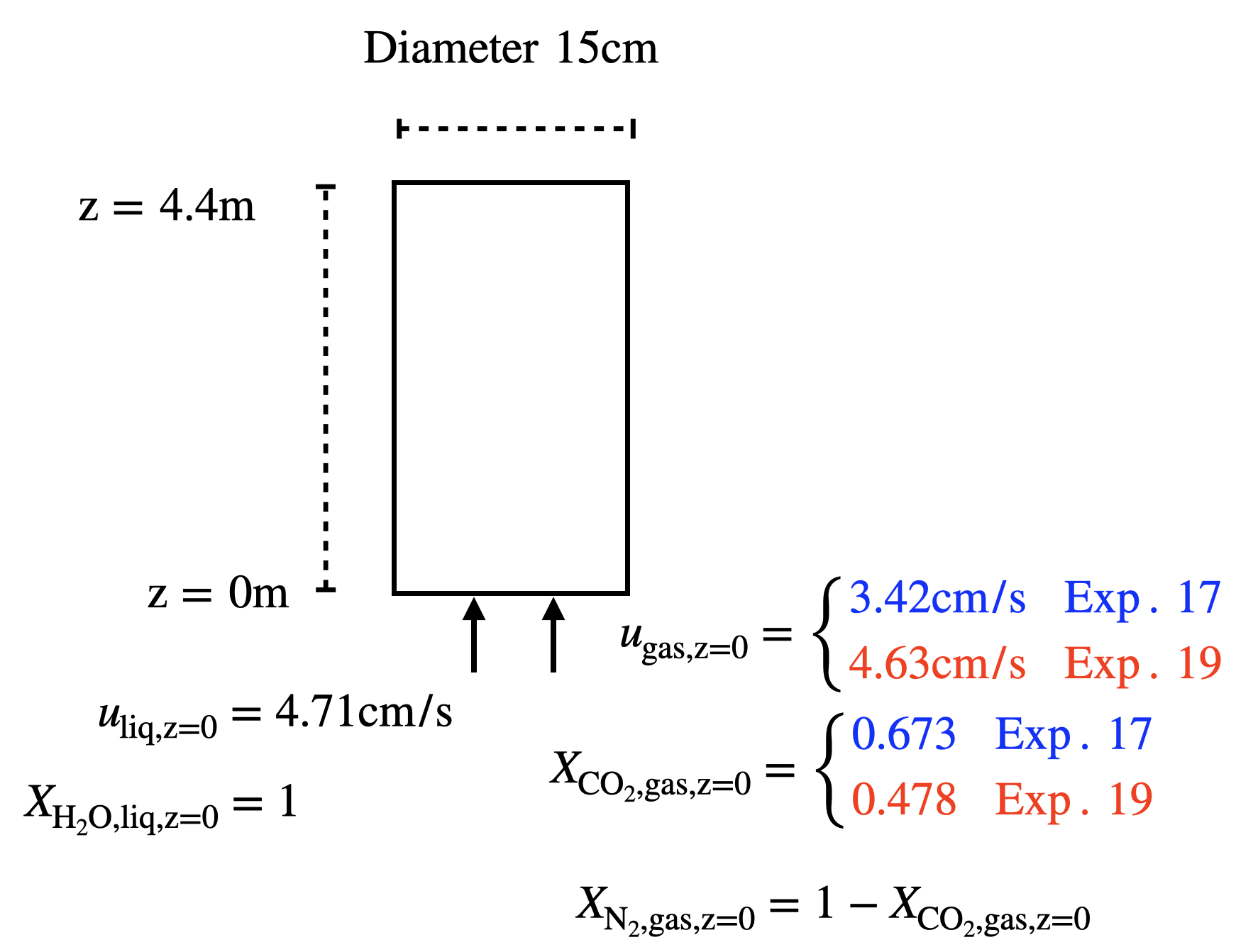
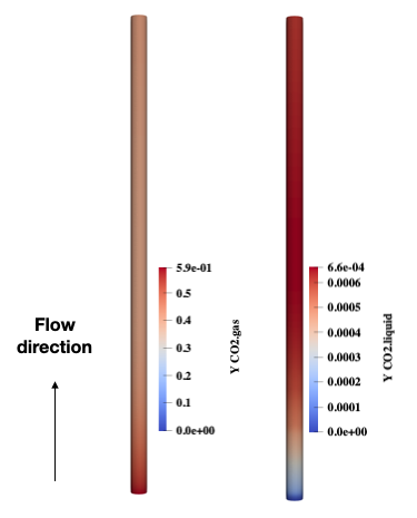
Figure 2: Left: schematic illustration of the case simulated with inlet conditions for Exp. 17 (blue) and Exp. 19 (red). Right: mass fraction of CO2 at steady state for Exp. 17 of Deckwer et al. [37] in the gas phase (left) and the liquid phase (right).

3.3 Comparison to experiments

The experimental measurements provide the average local gas holdup and CO2 gas concentration at different heights in the reactor. In the simulations, these quantities are reconstructed by performing a conditional average of gas volume fraction and CO2 mole fraction conditioned on the height coordinate (z). Figure 3 shows the comparison between simulations that were run with a global breakup model [17] and the experiments. For both the gas holdup and the CO2 gas mole fraction, the base simulation reasonably captures the experimental observations.

However significant differences can be observed especially for Exp. 19 for gas holdup and for Exp. 17 for CO2 gas concentration, especially near the top of the reactor. Other numerical investigations [58, 59] where a one-dimensional spatio-temporal approximation of the phase conservation equations was used, also deviate from experimental observations in a similar way.

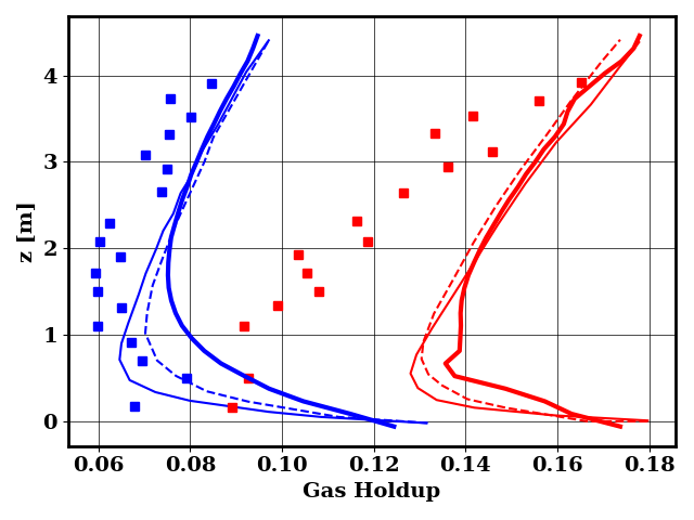
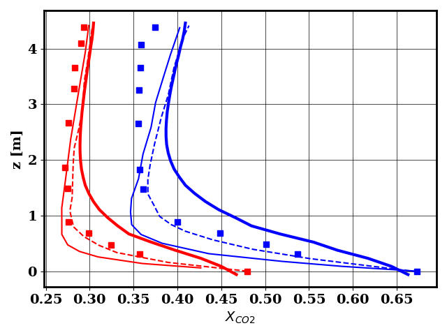
Figure 3: Height conditional average of gas holdup (left) and CO2 mole fraction in the gas phase (right) for experiments ( ) [37], Ref. [58] ( ), Ref. [59] ( ) and our results ( ), for Exp. 17 (blue) and Exp. 19 (red).

3.4 Source of discrepancy between numerical simulation and the experiments

Two reasons might explain the deviation between numerical simulations and experiments. First numerical errors may originate from the discretization of the domain and must be ruled out before considering model modifications [25]. A fine grid simulation was conducted using 176,400 cells (400 cells in the vertical direction, 28 in the azimuthal direction, and approximately 16 in the radial direction) compared to our baseline case with 64,800 cells, and a fine phase-space simulation was run using 20 bins for bubble-size discretization compared to 10 bins in the baseline case. In the fine grid simulation, the timestep is also based on the Courant number and is $1~{}\rm{ms}$ on average. As shown in Fig. 4, neither simulation deviated sufficiently from the base case to explain the discrepancy with experimental observations. Therefore, model errors are the likely cause of the discrepancy.

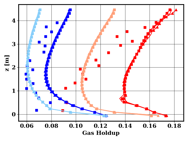
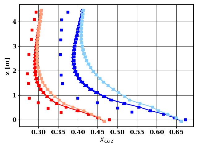
Figure 4: Height conditional average of gas holdup (left) and CO2 mole fraction in the gas phase (right) for experiments ( ) [37], coarse grid ( ), fine grid ( ), coarse grid with fine bubble size discretization ( ), for Exp. 17 (blue) and Exp. 19 (red). Dark lines: global breakup model [17]. Light lines: binary breakup model [56].

The same suite of runs (coarse and fine grids) was conducted with a binary breakup model [56] instead of a global breakup model [17]. This test serves here to understand how much variability can be expected due to a bubble size dynamics modeling error (similar to the approach of Mueller and Raman [60]). It can be seen in Fig. 4 that, once again, the numerical errors are unlikely to explain the discrepancy between numerical simulations and experiments. However, significant variability may be observed due to the modeling assumption adopted, and this variability may indeed close the gap to experimental observations.

4 Model calibration

In view of the results shown above, the modeling approach may explain the discrepancy with the experimental data. Therefore, we used the experiments of Deckwer et al. [37] to calibrate the breakup and coalescence models, in line with recommendations from previous research[16, 17, 18]. What is unique to the present study is that 1) the forward simulations are expensive (each forward run requires 360 CPU hours) and many runs were necessary to rule out numerical errors [25] and, 2) there appears to be irreducible discrepancies between some of the experimental data and numerical simulations. Therefore, the inclusion of experimental data in the calibration procedure requires taking into account those irreducible errors. In this section, the solutions to both issues are provided and exercised.

4.1 Calibration problem

Given the high computational expense required for evaluating the forward model, the calibration procedure should not involve too many parameters. The higher the dimension of the parameter space, the larger the number of forward model evaluations needed to explore the parameter space. Note that even if a surrogate model is used for the Bayesian inference, it would still need to be trained using data that span the entire parameter space [61]. Even when using faster forward models, other investigations have reduced the high-dimensional parameter space by assuming no joint effect of subsets of the entire parameter set [17].

In this work we calibrated 3 parameters: an efficiency factor for the coalescence kernel $C_{\rm eff}$, an efficiency factor for the breakup kernel $B_{\rm eff}$, and the surface tension $\Omega$. The base coalescence model is that of Lehr et al. [56]. For the breakup model, two separate corrections are derived for the global breakup model of Laakkonen et al. [17] and the binary breakup model of Lehr et al. [56].

The scaled coalescence and breakup kernels are expressed as

$$C_{\rm{corr},v^{\prime},v-v^{\prime}}=C_{\rm eff}C_{v^{\prime},v-v^{\prime}}$$ (11)

and

$$B_{\rm{corr},v}=B_{\rm eff}B_{v},$$ (12)

where $C_{\rm{corr},v^{\prime},v-v^{\prime}}$ and $B_{\rm{corr},v}$ are the corrected coalescence and breakup kernels and $C_{\rm eff}$ and $B_{\rm eff}$ are the unitless efficiency factors that scale the base models.

The choice of efficiency factors to calibrate the coalescence and breakup kernel is motivated by three reasons: 1) it allows to modulate the amplitude of the breakup and coalescence kernel by only manipulating one parameter which allows using a reduced number of forward evaluations; 2) the efficiency factor can be defined for any kernel functional which allows comparing different kernels and by how much each one must be corrected; 3) the efficiency factors are easily interpretable since their effect is linear on the frequency of breakup or coalescence.

Finally, the choice of calibrating surface tension $\Omega$ is motivated by the use of tap water in the experiments of Deckwer et al. [37]. The presence of surfactants in tap water could modify surface tension and thus can affect bubble size dynamics and mass transfer.

To decide what efficiency factors and surface tension values are most appropriate to explain the discrepancy between simulations and experimental observations, multiple simulations are run with different parameter values. A total of 120 numerical simulations were run with a coalescence/break-up efficiency factor varying in the range $[0.05,20]$, and tap water surface tension varying in the range $[0.03,0.11]\rm{N/m}$. The results are shown in Fig. 5 for the global breakup and are colored by the breakup efficiency factor value, indicating that the computed gas holdup and CO2 mole fraction axial profiles are sensitive to the model parameters varied.

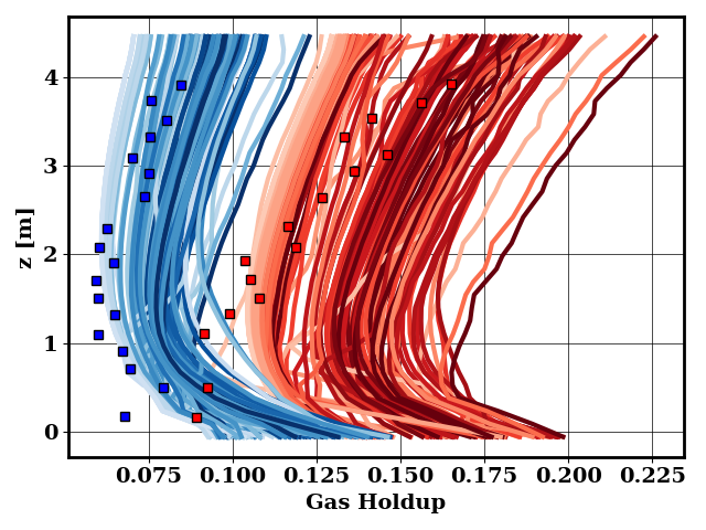
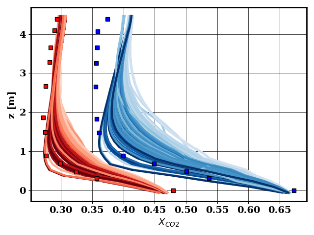
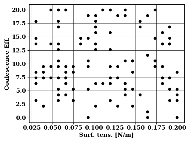
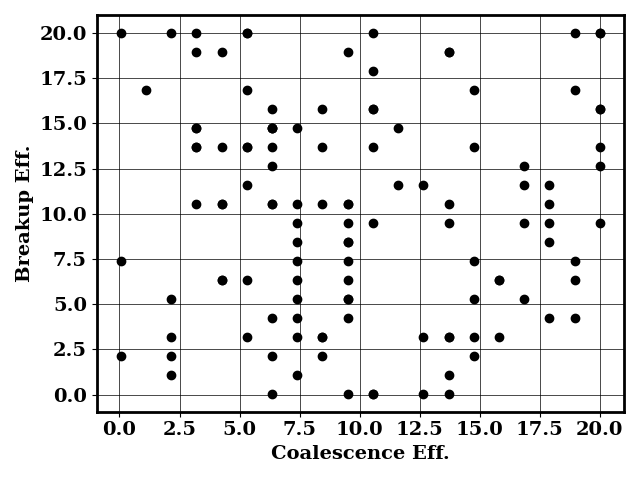
Figure 5: Top: Height conditional average of gas holdup (left) and CO2 mole fraction in the gas phase (right) for experiments ( ) [37], and simulated results using a global breakup model [17] ( ) for Exp. 17 (blue) and Exp. 19 (red). Darker colors denote the higher value of breakup efficiency. Bottom: scatter plot of the distribution of the 120 numerical simulations in the model parameter space for the global breakup model.

As suggested by the results of Sec. 3.4 the model parameter variation induces significant variability that could resolve part of the discrepancy to experimental observations. However, an optimal breakup efficiency factor is difficult to identify from Fig. 5. On the one hand, high values of the breakup efficiency factor improve the CO2 mole fraction prediction, while on the other hand, low values of breakup efficiency promotes a better match of gas holdup with experiments. In addition, there remain irreducible errors that cannot be mitigated through the variation of the parameters considered (see for instance gas CO2 concentration near the top of the reactor for Exp. 17). The same set of simulations resulted in similar conclusions when using the binary breakup kernel and is not described further for brevity.

4.2 Bayesian inference approach

To calibrate the chosen model parameters, while accounting for experimental uncertainty, a Bayesian calibration approach is used. In Bayesian calibration, the objective is to compute the posterior probability (or more commonly referred to as the posterior) of the parameters calibrated, denoted as $p_{\rm post}(\bm{p}|\bm{d})$, where $\bm{p}$ are the model parameters, and $\bm{d}$ are the experimental observations. The posterior $p_{\rm post}$ is obtained using the Bayes theorem

$$p_{\rm post}(\bm{p}|\bm{d})=\frac{p_{\rm prior}(\bm{p})p_{\rm like}(\bm{d}|\bm{p})}{p_{\rm evi}(\bm{d})},$$ (13)

where $p_{\rm prior}(\bm{p})$ is the prior probability that encodes prior knowledge about the parameters, and $p_{\rm like}(\bm{d}|\bm{p})$ is the likelihood function that characterizes how likely a parameter set $\bm{p}$ is to explain the observed data $\bm{d}$. The evidence $p_{\rm evi}(\bm{d})$ is shown for the sake of completeness but does not need to be defined for the Bayesian calibration procedure: it can be treated as a multiplicative factor independent of the parameters calibrated. Typically, the likelihood function is chosen to be a multivariate normal [32, 35, 34] defined by

$$p_{\rm like}(\bm{d}|\bm{p})=\frac{1}{(2\pi\sigma^{2})^{N_{\rm d}/2}}\times\ \exp\left[-\frac{1}{2\sigma^{2}}\sum_{i=1}^{N_{\rm d}}(\bm{d}-\bm{d}_{\rm pred}(\bm{p}))^{2}\right],$$ (14)

where $N_{\rm d}$ is the number of observations, $\sigma$ is the uncertainty in the experimental observations (where uncertainty is assumed to be the same for all observations), and $\bm{d}_{\rm pred}(\bm{p})$ is the prediction of observations that would be obtained if parameter set $\bm{p}$ was chosen.

The advantage of the Bayesian calibration is that the experimental uncertainty and the remaining model uncertainty that cannot be explained with the parameters calibrated can be lumped into the $\sigma$ uncertainty value of the likelihood function [35, 36] (see Sec. 4.4). Choosing a specific uncertainty for a specific experimental dataset allows to appropriately weight the experimental data, rather than averaging the error across all experimental data [22, 24].

4.3 Surrogate modeling approach

The main drawback of Bayesian calibration is its computational cost. The high cost of Bayesian calibration is due to evaluating the likelihood function. In the present case, it requires computing the prediction $\bm{d}_{\rm pred}(\bm{p})$ which would necessitate a forward model evaluation (here running a CFD simulation). To accelerate the Bayesian calibration, the function $\bm{d}_{\rm pred}(\bm{p})$ can, however, be approximated with a data-based model which was trained, in our case using the 120 simulations shown in Fig. 5. Other uncertainty quantification approaches that require multiple forward model evaluation adopt similar strategies [62, 63].

Here, the surrogate models are constructed using a fully connected neural network schematically illustrated in Fig. 6(a). The neural net contains four inputs: the vertical direction $z$ and the three calibrated model parameters ($C_{\rm eff}$, $B_{\rm eff}$ and $\Omega$). The output of the neural net is one dimensional and consists of either the gas-holdup or the gas molar fraction of CO2. In total, eight different surrogate models were trained, a different one for each measured quantity (gas hold up or CO2 mole fraction), each experiment (Exp. 17 or Exp. 19), and each breakup kernel (binary or global). For each surrogate model, 32 conditional average points are drawn for each simulation which amounts to 3840 data points per surrogate. One percent of the data is reserved for validation. For simplification, all surrogate models used the same hyperparameters that are summarized in Tab. 1(a). The neural nets were trained with a classical mean-square error loss. Further details on the effect of the epoch number are provided in A.

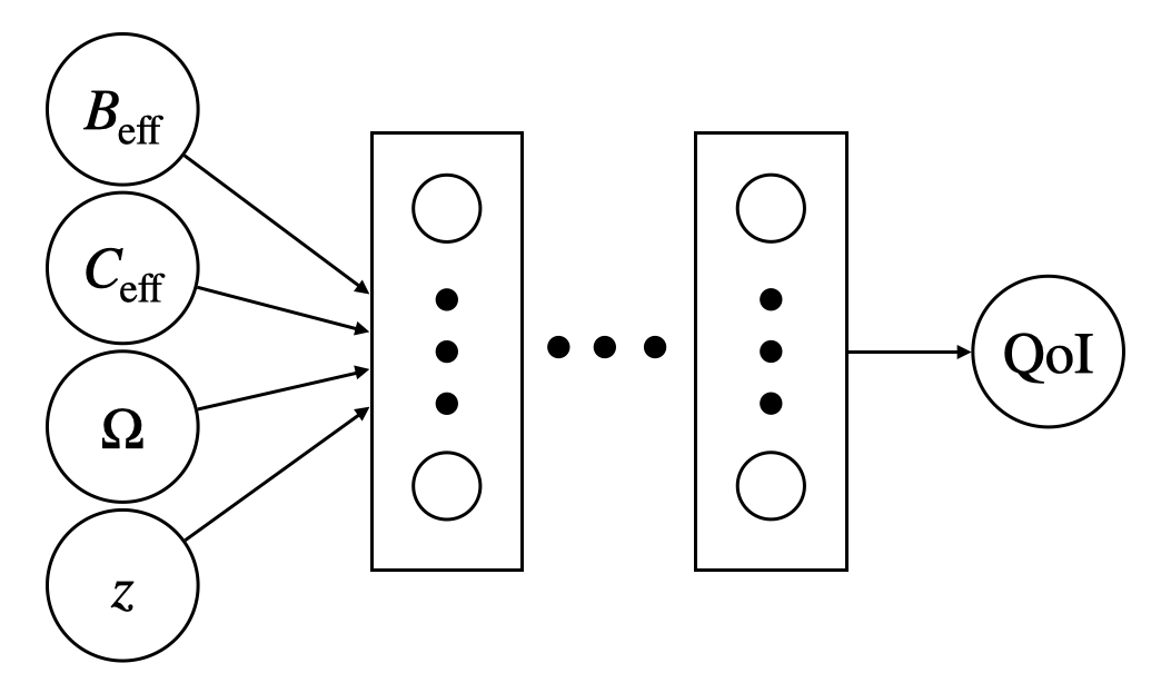
(a) Input output mapping of each surrogate model. Each surrogate take 4 input and output only one output denoted by QoI.

Name	Value
Hidden layer size	{ 10, 20, 10, 5}
Activation	tanh
Batch size	32
Learning rate	$1\mathrm{e}{-03}$
Epochs	1000

(a) Hyperparameters used for the neural net surrogates. The hidden layer size denotes the number of neurons in the 4 hidden layers used.

Figure 6: Architecture of the neural network surrogates.

The surrogate model can be used to compute the likelihood function $p_{\rm like}(\bm{d}|\bm{p})$. To perform Bayesian calibration, the prior distribution of the parameters must also be chosen. In order to use the surrogate model, the support of the priors cannot be larger than the input feature intervals over which the surrogate was trained. The priors for the coalescence and the breakup efficiency factor are chosen to be uniform distributions $\mathcal{U}(0.05,20)$, whose support is the same as the interval over which the surrogate was trained. In general, the magnitude of the breakup kernels adopted does not vary by a factor greater than 20 [21]. The priors adopted reflect that scaling the coalescence and breakup kernel by a factor greater than 20 is unreasonable. The prior for the surface tension is chosen to be $\mathcal{U}(0.065,0.075)$ N/m. Given available estimates of the surface tension of tap water [64, 65], the support of the surface tension prior was made tighter than the interval over which the surrogate was trained.

4.4 Combining multiple observations

As mentioned in Sec. 1.1, it is common practice to calibrate bubble size dynamics models against the simulation of experimental observations, by uniformly weighting the errors to experimental data [22, 24, 27]. This approach implicitly assumes that all experiments are equally informative to calibrating model parameters. However, different experiments may be subject to different levels of noise, especially when different variables are measured. For instance, Fig. 4 suggests that the noise-to-signal ratio is larger for the gas holdup compared to CO2 mole fraction. Furthermore, despite pushing the parameters to calibrate to their limit, there remain irreducible discrepancies between some experiments and simulations results (Fig. 5). In these cases, to match such experimental observations, the models need to be equipped with additional physics that are missing. The missing physics could be because of inherent model deficiencies, or because the experiments were affected by unknown or undocumented variables. Either way, the missing physics makes the experimental observation less informative about the parameters being calibrated. Figure 7 schematically illustrates the missing physics issue. To account for the missing physics, the likelihood uncertainty $\sigma$ (Eq. 14) can be adjusted to reflect the fact some experiments are less informative for the parameter calibration. In Fig. 7, the likelihood uncertainty is plotted as an experimental uncertainty (red dashed lined) that contains the noise and the missing physics. Hereafter, the likelihood uncertainty is assumed uniform for each one of the four experimental datasets: a single likelihood uncertainty is used for each measurement type ($X_{\ce{CO2}}$, gas holdup) and each experimental campaign (Exp. 17 and Exp. 19).

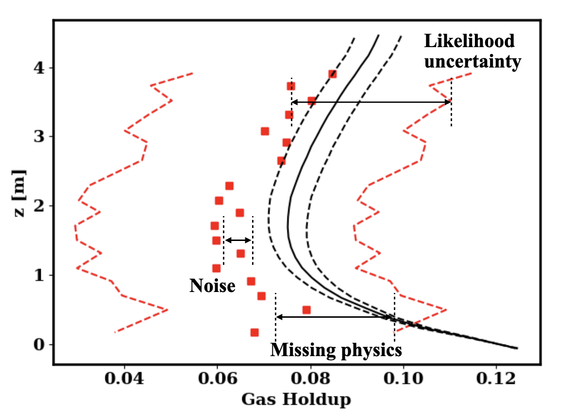
Figure 7: Illustration of the missing physics issue. If experimental noise and model parameter uncertainty (black dashed lines) are not necessary to explain discrepancies between simulation and experiments, a missing physics component is added to the likelihood uncertainty (red dashed lines).

To set the likelihood uncertainty so as to reflect both the experimental noise and the missing physics, two different methods are used. First, the Bayesian calibration can be done for each one of the four experimental datasets while calibrating the likelihood uncertainty along with the physical parameters (coalescence efficiency, breakup efficiency, surface tension). As a second step, the mean likelihood uncertainty of each one of the four experimental datasets is gathered and used to perform the final calibration that combines all experimental data. This procedure is summarized in Algo. 1 where $\mathbb{E}_{p_{\rm post}}(\sigma)$ denotes the average of the likelihood $\sigma$ averaged over the posterior probability sampled.

Algorithm 1 Likelihood uncertainty calibration.

1:for $\text{Exp}_{\rm i}$ $\in$ { Exp. 17 Gas Holdup, Exp. 17 $X_{\ce{CO2}}$, Exp. 19 Gas Holdup, Exp. 19 $X_{\ce{CO2}}$ } do

2:     Calibrate $B_{\rm eff}$, $C_{\rm eff}$, $\Omega$ and $\sigma$

3:     Compute $\sigma_{i}=\mathbb{E}_{p_{\rm post,i}}(\sigma)$

4:end for

Second, the likelihood uncertainty can be treated as a hyperparameter that needs to be optimized. Qualitatively, the uncertainty band obtained by calibrating the model parameters (black dashed lines in Fig. 7) must be contained in the likelihood uncertainty assigned to the experiments (the red dashed lines in Fig. 7). The definition of uncertainty bands is arbitrary and is chosen to be the $95\%$ confidence interval for the experiments, and the $95\%$ confidence interval for the model predictions. Formally, the likelihood uncertainty $\sigma_{i}$ is chosen by solving the following optimization problem for each experiment $i$

$$\min_{\sigma_{i}}$$ (15)

s.t. $$V_{i,j}+2\sigma_{i}>P_{i,j,97.5}(\sigma_{i}),~{}\forall j$$

$$V_{i,j}-2\sigma_{i}<P_{i,j,2.5}(\sigma_{i}),~{}\forall j,$$

where $V_{i,j}$ is the $j^{th}$ measurement of experimental dataset $i$, $P_{i,j,97.5}$ (resp. $P_{i,j,2.5}$) is the 97.5^th (resp. 2.5^th) percentile of the model predictions for the $j^{th}$ measurement of experiment $i$ obtained by sampling the posterior of $B_{\rm eff}$, $C_{\rm eff}$ and $\Omega$.

The optimal value of the likelihood uncertainty can be iteratively searched, where each iteration consists in choosing a value of $\sigma_{i}$ and calibrating the model parameters ($B_{\rm eff}$, $C_{\rm eff}$, $\Omega$) using $\sigma_{i}$ as likelihood uncertainty. Since a surrogate model is used in place of the physics model, the calibration process is sufficiently cheap to allow performing multiple calibrations. The procedure is summarized in Algo. 2.

Algorithm 2 Likelihood uncertainty optimization.

1:for $\text{Exp}_{\rm i}$ $\in$ { Exp. 17 Gas Holdup, Exp. 17 $X_{\ce{CO2}}$, Exp. 19 Gas Holdup, Exp. 19 $X_{\ce{CO2}}$ } do

2:     Solve Eq.15 via a bisection method

3:     Store the solution $\sigma_{i}$ for $\text{Exp}_{\rm i}$.

4:end for

The likelihood uncertainties obtained with both methods are shown in Tab. 2 for the Binary breakup and the global breakup model. Overall, the uncertainties predicted with both methods are in agreement with each other, which suggests that calibrating likelihood uncertainties is equivalent to solving the optimization problem shown in Eq. 15. Importantly, calibrating the likelihood uncertainties only requires one calibration procedure per experiment, while 10 were used for the hyperparameter search.

The likelihood uncertainties reflect the amount of noise in the experimental data as well as the amount of physics missing to explain the experiments with the models. By comparing the likelihood uncertainties across modeling assumptions (global breakup or binary breakup assumption), one can compare the amount of physics missing in each model, irrespective of the calibrated model parameters. This is possible here since the breakup model is the only modeling choice varied, while the coalescence model is the same. Other Bayesian model ranking strategies have been proposed [32] by accounting for the amount of parameter tuning needed for each model. A simpler model ranking method is used here since both models need to be tuned by the same amount (see Sec. 4.5). Here, it appears that the global breakup model is about two times more accurate than the binary breakup model for $X_{\ce{CO2}}$ and is only 10-20% less accurate than the binary breakup model for gas holdup.

	Exp. 17		Exp. 19
	$X_{CO_{2}}$	Gas Holdup	$X_{CO_{2}}$	Gas Holdup
Binary Breakup	0.058	0.009	0.03	0.016
Global Breakup	0.034	0.008	0.015	0.02

(a) Likelihood uncertainties obtained using Algo. 1.

	Exp. 17		Exp. 19
	$X_{CO_{2}}$	Gas Holdup	$X_{CO_{2}}$	Gas Holdup
Binary Breakup	0.066	0.009	0.039	0.024
Global Breakup	0.025	0.010	0.015	0.027

(b) Likelihood uncertainties obtained using Algo. 2.

Table 2: Optimal likelihood uncertainty for each experimental dataset and each breakup model.

Given that interphase mass transfer is a critical parameter for CO2 gas fermenters, accurate predictions of the gas mole fraction $X_{\ce{CO2}}$ are needed. The calibrated and optimized likelihood uncertainties suggest that irrespective of efficiency parameter calibration, a global breakup model [17] is more appropriate to capture the experimental interphase mass transfer observed compared to the binary breakup model [56].

4.5 Results

The Bayesian calibration is conducted using Hamiltonian Monte-Carlo (HMC) [66, 67] which is made possible due to the auto-differentiation capability of the neural network surrogate. The likelihood uncertainties obtained with the calibration (Algo. 1) and the optimization method (Algo. 2) are used to compute the likelihood function that combines all the experiments. One calibration is done with the global breakup model and one with the binary breakup model. Figure 8 shows the posterior probability density function (PDF) of the calibrated parameters obtained when combining all the experiments and using the likelihood uncertainties computed via the optimization method (Algo. 2). The posteriors obtained when using the likelihood uncertainties computed via the calibration method (Algo. 1) are similar and are not shown here for the sake of concision.

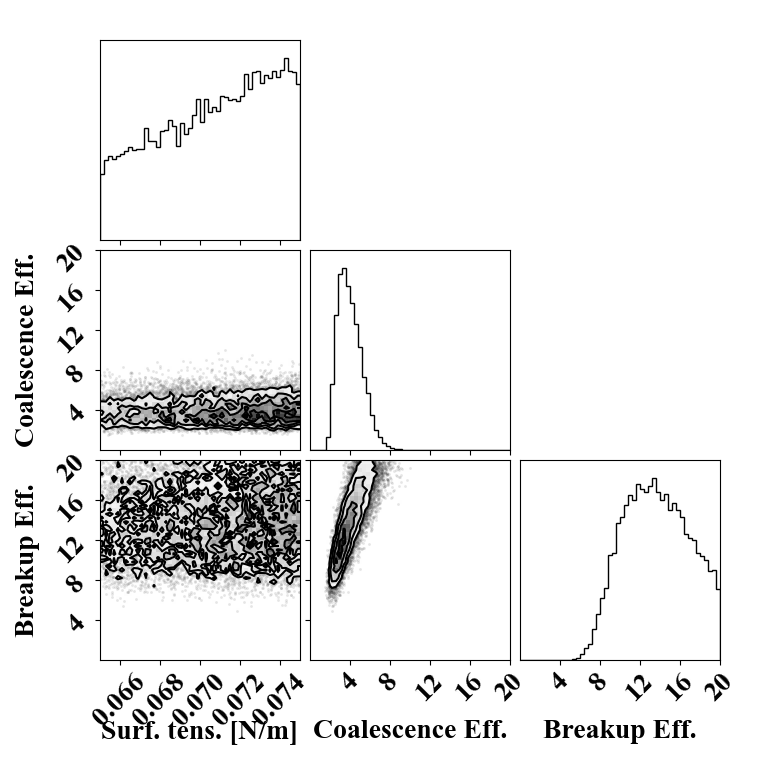
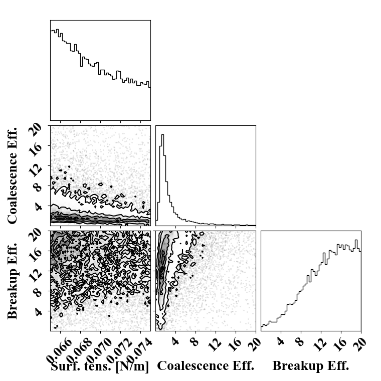
Figure 8: Corner plots of the posterior probability obtained for the global breakup model [17] (left) and the binary breakup model [56] (right).

First, it appears that any value of surface tension within the interval chosen is reasonable to explain the discrepancy with experimental data. Therefore the experimental data is not sufficient to confidently decide whether the surface tension of tap water was affected by surfactants. However, only narrow regions of the coalescence and breakup efficiency domain of definition are likely. The coalescence efficiency is found most likely between 2 and 4, while the breakup efficiency is found most likely between values 10 and 15. Remarkably, both breakup models (global and binary) land on similar conclusions regarding the posterior probability. The posterior exhibits a correlation between coalescence and breakup efficiencies which can be understood by the fact that higher breakup rates may be compensated by higher coalescence rates. The agreement of the calibrated efficiency factors suggests that the model correction are a) either needed for modeling the bubble dynamics of gaseous CO2; or b) needed to model the specific experiment simulated here. A definitive conclusion would require performing the same calibration exercise with several other experimental campaign measurements, and is left for future work.

A last set of simulations, termed a posteriori runs, was performed to verify the predictions of the optimized models. A binary breakup model was used with coalescence efficiency factor $C_{\rm eff}=1.83$ and breakup efficiency factor $B_{\rm eff}=13.565$ and a global breakup model was used with $C_{\rm eff}=4.695$ and $B_{\rm eff}=13.83$. The values chosen correspond to the posterior means of $B_{\rm eff}$ and $C_{\rm eff}$. Figure 9 shows the predicted results of the optimized models against the base models using the baseline computational grid and bubble size discretizations (Sec. 3.4). In the case of the binary breakup model, the optimized model mostly affected the gas holdup prediction, especially for Exp. 19. However, the gas mole fraction concentrations are left almost unchanged. This is a consequence of the relatively high likelihood uncertainty for $X_{\ce{CO2}}$ which leads to prioritize gas holdup in the model calibration. The opposite effect can be seen for the global breakup model where significant improvement can be observed for $X_{\ce{CO2}}$ while gas holdup is unchanged or even less accurate (especially for Exp. 17). Overall, the calibration using the neural network surrogate is consistent with the a posteriori runs, which confirms that the neural network surrogate was sufficiently accurate.

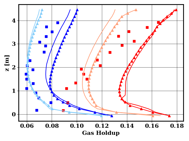
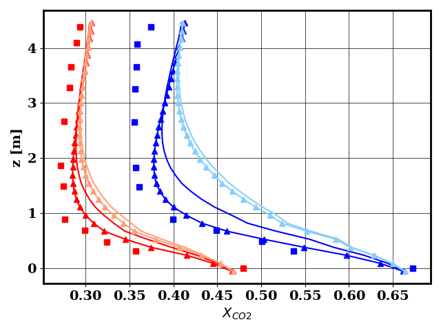
Figure 9: Height conditional average of gas holdup (left) and CO2 mole fraction in the gas phase (right) for experiments ( ) [37], the base model ( ), the calibrated model ( ) for Exp. 17 (blue) and Exp. 19 (red). Dark lines: global breakup model [17]. Light lines: binary breakup model [56].

5 Conclusions

In this work, an inverse modeling procedure was conducted to calibrate bubble size dynamics models against experimental measurements of a coflowing bubble column reactor.

Experimental noise and simulation bias were accounted for using a Bayesian inference approach. Given the common practice of calibrating bubble size dynamics model parameters, choosing an appropriate model functional form, irrespective of the parameter calibration is non-trivial. Here, it is shown that estimating the simulation bias allows one to discriminate between modeling approaches. In the present case, a global breakup modeling approach proved more appropriate for capturing interphase mass transfer, which is essential for gas fermentation applications. The simulation bias can be estimated either by including the likelihood uncertainty in the set of calibrated parameters, or by treating the likelihood uncertainty as a hyperparameter.

For computational tractability, the Bayesian inference needs to be paired with a surrogate model rather than a physics model. It was shown that a simple neural network was able to approximate the dependence of the model prediction with respect to the model parameters inferred.

The calibration results show that for both global breakup and binary breakup modeling approaches, the magnitude of the breakup kernel needs to be increased by about one order of magnitude. Since both modeling approaches led to similar conclusions, either the breakup dynamics of CO2 gas are atypical, or an element of the experimental apparatus promoted high breakage rates. A definitive conclusion would require exercising the calibration method described against a larger experimental dataset.

Appendix A Convergence of the neural networks

Figure 10 shows the training and validation loss history of the neural network surrogate of the breakup model and of the binary breakup model. Overall, it can be seen that the training and testing loss are nearly converged. Since the testing losses do not gradually increase with the epoch number, the surrogates are unlikely to overfit.

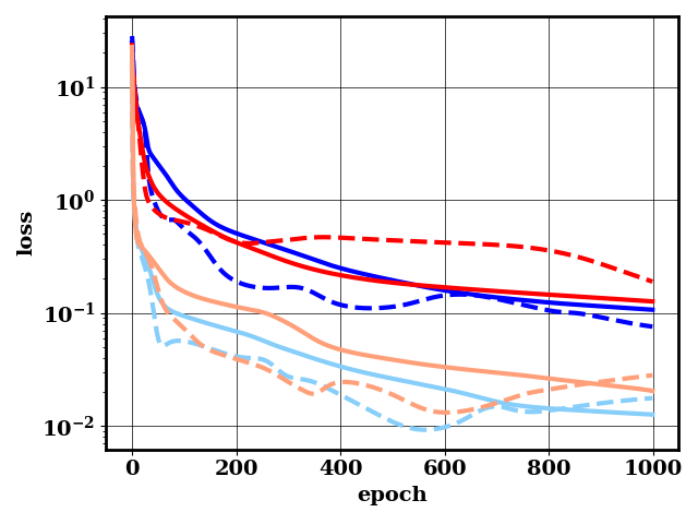
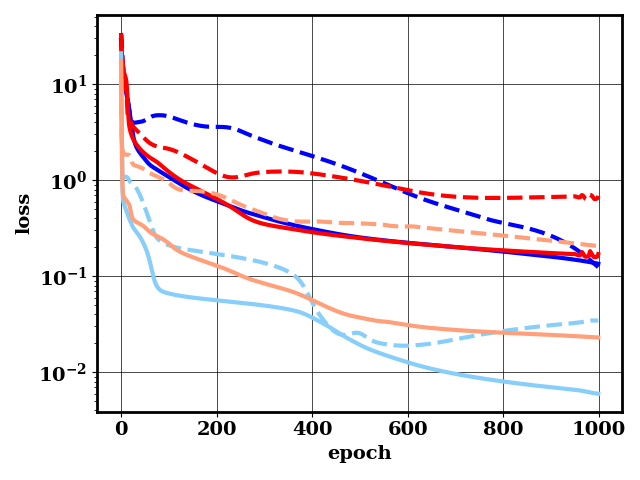
Figure 10: Training ( ) and testing ( ) loss history of the neural network surrogates trained on the Exp. 17 ( ) and Exp. 19 ( ), for the global breakup model [17] (left) and the binary breakup model [56] (right). Dark lines: gas holdup. Light lines: CO2 gas mole fraction.

Appendix B Turbulence boundary conditions

The turbulent boundary conditions for the turbulent kinetic energy $k$ and the turbulent energy dissipation rate $\varepsilon$ were artificially increased in the present work (Sec. 3.3, Sec. 3.4 and Sec. 4) for stability reasons. The chosen turbulent inlet boundary conditions are reported in Tab. 3, along with theoretical values for freestream turbulence, assuming 5% turbulence intensity in the liquid phase and the gas phase.

	Exp. 17		Exp. 19
	Gas	Liquid	Gas	Liquid
This work	3.7e-5	0.01	3.7e-5	0.01
Turbulence intensity 5%	4.4e-6	8.3e-6	8.0e-6	8.3e-6

(a) Turbulent kinetic energy boundary conditions in $m^{2}.s^{-2}$.

	Exp. 17		Exp. 19
	Gas	Liquid	Gas	Liquid
This work	1.5e-4	1.5e-4	1.5e-4	1.5e-4
Turbulence intensity 5%	1.44e-7	3.75e-7	3.6e-7	3.75e-7

(b) Turbulent kinetic energy dissipation rate boundary conditions in $m^{2}.s^{-3}$.

Table 3: Comparison of turbulent inlet boundary conditions between the cases simulated and a case assuming 5% turbulence intensity.

The same numerical simulations as the coarse grid case in Sec. 3.4 were performed with freestream turbulence boundary conditions, assuming 5% turbulence intensity. The results are shown in Fig. 11 for gas holdup only for concision. It can be seen that using the non-artificially increased turbulent boundary conditions leads to spurious oscillations for the global breakup model. However, the results are almost unchanged for the binary breakup case. In Fig. 11 (right) it is clear that the turbulent kinetic energy in the liquid phase rapidly deviates from the freestream boundary conditions because of the walls, and reaches levels higher than the artificially increased turbulent kinetic energy boundary conditions. Therefore, although the inlet boundary conditions chosen are inaccurate, they are unlikely to affect the results reported (aside from providing increased stability).

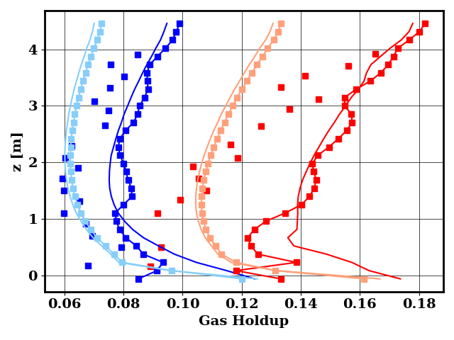
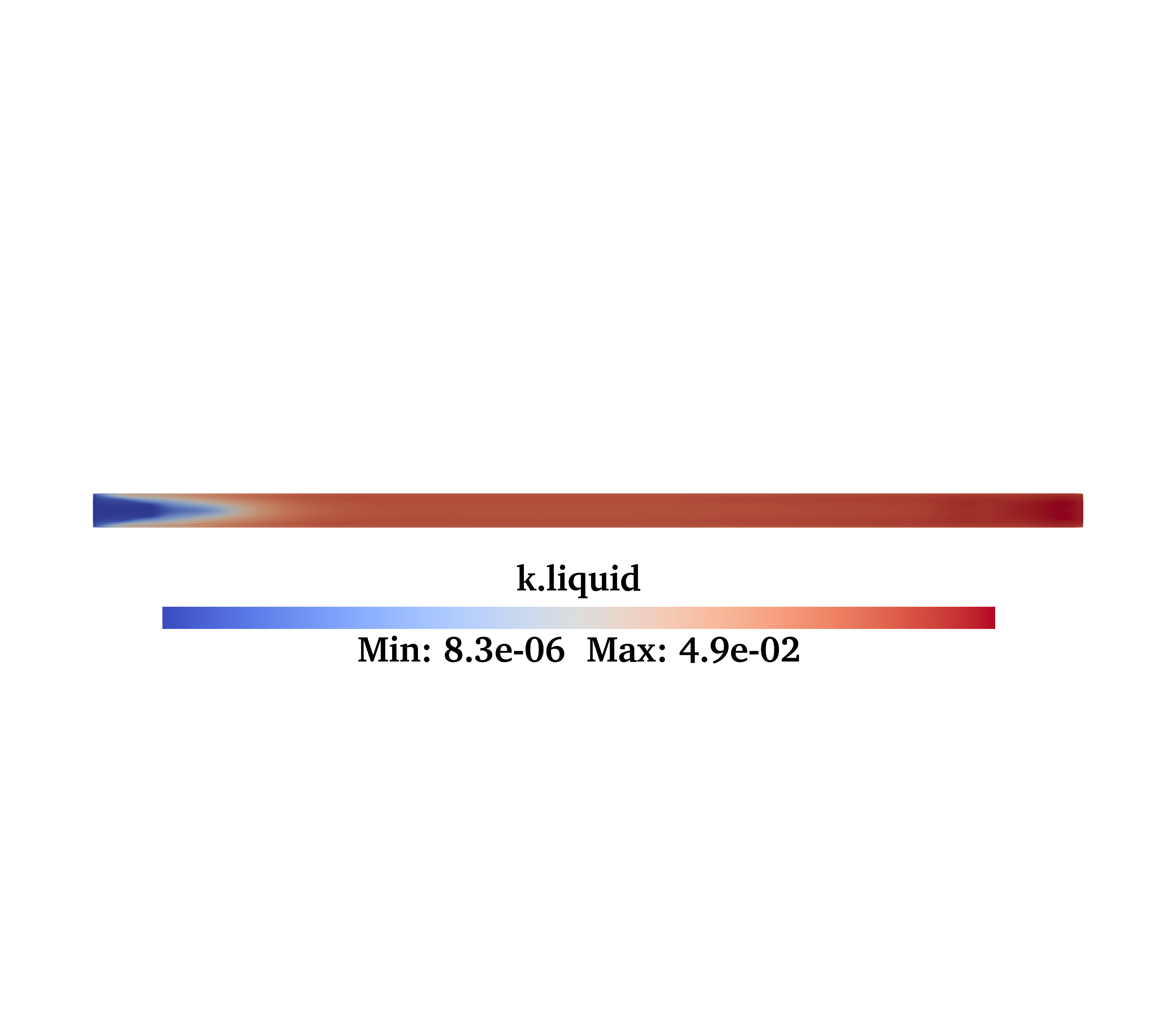
Figure 11: Left: Height conditional average of gas holdup for experiments ( ) [37], results using artificially high turbulent inlet boundary conditions ( ), results using freestream turbulence inlet boundary conditions with 5% turbulence intensity ( ) for Exp. 17 (blue) and Exp. 19 (red). Right: contour of the liquid turbulent kinetic energy for Exp. 17 using freestream turbulence inlet boundary conditions with 5% turbulence intensity and the non-modified binary breakup model [56]. The flow goes from left to right.

References

- Lee et al. [2023] \bibinfoauthorH. Lee, \bibinfoauthorK. Calvin, \bibinfoauthorD. Dasgupta, \bibinfoauthorG. Krinner, \bibinfoauthorA. Mukherji, \bibinfoauthorP. Thorne, \bibinfoauthorC. Trisos, \bibinfoauthorJ. Romero, \bibinfoauthorP. Aldunce, \bibinfoauthorK. Barret, et al., \bibinfotitleIPCC, 2023: Climate Change 2023: Synthesis Report, Summary for Policymakers. Contribution of Working Groups I, II and III to the Sixth Assessment Report of the Intergovernmental Panel on Climate Change (\bibinfoyear2023).
- Bergero et al. [2023] \bibinfoauthorC. Bergero, \bibinfoauthorG. Gosnell, \bibinfoauthorD. Gielen, \bibinfoauthorS. Kang, \bibinfoauthorM. Bazilian, \bibinfoauthorS. J. Davis, \bibinfotitlePathways to net-zero emissions from aviation, \bibinfojournalNature Sustainability \bibinfovolume6 (\bibinfoyear2023) \bibinfopages404–414.
- Schwab et al. [2021] \bibinfoauthorA. Schwab, \bibinfoauthorA. Thomas, \bibinfoauthorJ. Bennett, \bibinfoauthorE. Robertson, \bibinfoauthorS. Cary, \bibinfotitleElectrification of aircraft: Challenges, barriers, and potential impacts, \bibinfotypeTechnical Report, National Renewable Energy Lab.(NREL), Golden, CO (United States), \bibinfoyear2021.
- Shahriar and Khanal [2022] \bibinfoauthorM. F. Shahriar, \bibinfoauthorA. Khanal, \bibinfotitleThe current techno-economic, environmental, policy status and perspectives of sustainable aviation fuel (SAF), \bibinfojournalFuel \bibinfovolume325 (\bibinfoyear2022) \bibinfopages124905.
- Grim et al. [2023] \bibinfoauthorR. G. Grim, \bibinfoauthorJ. R. Ferrell III, \bibinfoauthorZ. Huang, \bibinfoauthorL. Tao, \bibinfoauthorM. G. Resch, \bibinfotitleThe feasibility of direct CO2 conversion technologies on impacting mid-century climate goals, \bibinfojournalJoule \bibinfovolume7 (\bibinfoyear2023) \bibinfopages1684–1699.
- Tarraran et al. [2023] \bibinfoauthorL. Tarraran, \bibinfoauthorV. Agostino, \bibinfoauthorN. S. Vasile, \bibinfoauthorA. A. Azim, \bibinfoauthorG. Antonicelli, \bibinfoauthorJ. Baker, \bibinfoauthorJ. Millard, \bibinfoauthorA. Re, \bibinfoauthorB. Menin, \bibinfoauthorT. Tommasi, et al., \bibinfotitleHigh-pressure fermentation of CO2 and H2 by a modified Acetobacterium woodii, \bibinfojournalJournal of CO2 Utilization \bibinfovolume76 (\bibinfoyear2023) \bibinfopages102583.
- Straub et al. [2014] \bibinfoauthorM. Straub, \bibinfoauthorM. Demler, \bibinfoauthorD. Weuster-Botz, \bibinfoauthorP. Dürre, \bibinfotitleSelective enhancement of autotrophic acetate production with genetically modified Acetobacterium woodii, \bibinfojournalJournal of Biotechnology \bibinfovolume178 (\bibinfoyear2014) \bibinfopages67–72.
- Pfeifer et al. [2021] \bibinfoauthorK. Pfeifer, \bibinfoauthorİ. Ergal, \bibinfoauthorM. Koller, \bibinfoauthorM. Basen, \bibinfoauthorB. Schuster, \bibinfoauthorK.-M. R. Simon, \bibinfotitleArchaea biotechnology, \bibinfojournalBiotechnology Advances \bibinfovolume47 (\bibinfoyear2021) \bibinfopages107668.
- Yan et al. [2023] \bibinfoauthorS.-l. Yan, \bibinfoauthorX.-q. Wang, \bibinfoauthorL.-t. Zhu, \bibinfoauthorX.-b. Zhang, \bibinfoauthorZ.-h. Luo, \bibinfotitleMechanisms and modeling of bubble dynamic behaviors and mass transfer under gravity: a review, \bibinfojournalChemical Engineering Science (\bibinfoyear2023) \bibinfopages118854.
- McGraw [1997] \bibinfoauthorR. McGraw, \bibinfotitleDescription of aerosol dynamics by the quadrature method of moments, \bibinfojournalAerosol Science and Technology \bibinfovolume27 (\bibinfoyear1997) \bibinfopages255–265.
- Krepper et al. [2007] \bibinfoauthorE. Krepper, \bibinfoauthorT. Frank, \bibinfoauthorD. Lucas, \bibinfoauthorH.-M. Prasser, \bibinfoauthorP. J. Zwart, \bibinfotitleInhomogeneous MUSIG model - a population balance approach for polydispersed bubbly flows, in: \bibinfobooktitleThe 12th International Topical Meeting on Nuclear Reactor Thermal Hydraulics (NURETH-12), volume \bibinfovolume30, \bibinfoyear2007, p. \bibinfopages2007.
- Lo [1996] \bibinfoauthorS. Lo, \bibinfotitleApplication of population balance to CFD modeling of bubbly flow via the MUSIG model, \bibinfoyear1996.
- Gao et al. [2016] \bibinfoauthorZ. Gao, \bibinfoauthorD. Li, \bibinfoauthorA. Buffo, \bibinfoauthorW. Podgórska, \bibinfoauthorD. L. Marchisio, \bibinfotitleSimulation of droplet breakage in turbulent liquid–liquid dispersions with CFD-PBM: Comparison of breakage kernels, \bibinfojournalChemical Engineering Science \bibinfovolume142 (\bibinfoyear2016) \bibinfopages277–288.
- Kálal et al. [2014] \bibinfoauthorZ. Kálal, \bibinfoauthorM. Jahoda, \bibinfoauthorI. Fořt, \bibinfotitleModelling of the bubble size distribution in an aerated stirred tank: Theoretical and numerical comparison of different breakup models, \bibinfojournalChemical and Process Engineering (\bibinfoyear2014) \bibinfopages331–348.
- Wang et al. [2005] \bibinfoauthorT. Wang, \bibinfoauthorJ. Wang, \bibinfoauthorY. Jin, \bibinfotitlePopulation balance model for gas- liquid flows: Influence of bubble coalescence and breakup models, \bibinfojournalIndustrial & Engineering Chemistry Research \bibinfovolume44 (\bibinfoyear2005) \bibinfopages7540–7549.
- Laakkonen et al. [2006] \bibinfoauthorM. Laakkonen, \bibinfoauthorV. Alopaeus, \bibinfoauthorJ. Aittamaa, \bibinfotitleValidation of bubble breakage, coalescence and mass transfer models for gas–liquid dispersion in agitated vessel, \bibinfojournalChemical Engineering Science \bibinfovolume61 (\bibinfoyear2006) \bibinfopages218–228.
- Laakkonen et al. [2007] \bibinfoauthorM. Laakkonen, \bibinfoauthorP. Moilanen, \bibinfoauthorV. Alopaeus, \bibinfoauthorJ. Aittamaa, \bibinfotitleModelling local bubble size distributions in agitated vessels, \bibinfojournalChemical Engineering Science \bibinfovolume62 (\bibinfoyear2007) \bibinfopages721–740.
- Singh et al. [2009] \bibinfoauthorK. Singh, \bibinfoauthorS. Mahajani, \bibinfoauthorK. Shenoy, \bibinfoauthorS. Ghosh, \bibinfotitlePopulation balance modeling of liquid- liquid dispersions in homogeneous continuous-flow stirred tank, \bibinfojournalIndustrial & Engineering Chemistry research \bibinfovolume48 (\bibinfoyear2009) \bibinfopages8121–8133.
- Alopaeus et al. [2002] \bibinfoauthorV. Alopaeus, \bibinfoauthorJ. Koskinen, \bibinfoauthorK. I. Keskinen, \bibinfoauthorJ. Majander, \bibinfotitleSimulation of the population balances for liquid–liquid systems in a nonideal stirred tank. Part 2—parameter fitting and the use of the multiblock model for dense dispersions, \bibinfojournalChemical Engineering Science \bibinfovolume57 (\bibinfoyear2002) \bibinfopages1815–1825.
- Ruiz and Padilla [2005] \bibinfoauthorM. Ruiz, \bibinfoauthorR. Padilla, \bibinfotitleDetermination of coalescence functions in liquid–liquid dispersions, \bibinfojournalHydrometallurgy \bibinfovolume80 (\bibinfoyear2005) \bibinfopages32–42.
- Azizi and Al Taweel [2011] \bibinfoauthorF. Azizi, \bibinfoauthorA. Al Taweel, \bibinfotitleTurbulently flowing liquid–liquid dispersions. Part I: drop breakage and coalescence, \bibinfojournalChemical Engineering Journal \bibinfovolume166 (\bibinfoyear2011) \bibinfopages715–725.
- Castellano et al. [2019] \bibinfoauthorS. Castellano, \bibinfoauthorL. Carrillo, \bibinfoauthorN. Sheibat-Othman, \bibinfoauthorD. Marchisio, \bibinfoauthorA. Buffo, \bibinfoauthorS. Charton, \bibinfotitleUsing the full turbulence spectrum for describing droplet coalescence and breakage in industrial liquid-liquid systems: Experiments and modeling, \bibinfojournalChemical Engineering Journal \bibinfovolume374 (\bibinfoyear2019) \bibinfopages1420–1432.
- Sathyagal et al. [1995] \bibinfoauthorA. Sathyagal, \bibinfoauthorD. Ramkrishna, \bibinfoauthorG. Narsimhan, \bibinfotitleSolution of inverse problems in population balances-II. Particle break-up, \bibinfojournalComputers & Chemical Engineering \bibinfovolume19 (\bibinfoyear1995) \bibinfopages437–451.
- Mignard et al. [2006] \bibinfoauthorD. Mignard, \bibinfoauthorL. P. Amin, \bibinfoauthorX. Ni, \bibinfotitleDetermination of breakage rates of oil droplets in a continuous oscillatory baffled tube, \bibinfojournalChemical Engineering Science \bibinfovolume61 (\bibinfoyear2006) \bibinfopages6902–6917.
- Maluta et al. [2021] \bibinfoauthorF. Maluta, \bibinfoauthorA. Buffo, \bibinfoauthorD. Marchisio, \bibinfoauthorG. Montante, \bibinfoauthorA. Paglianti, \bibinfoauthorM. Vanni, \bibinfotitleEffect of turbulent kinetic energy dissipation rate on the prediction of droplet size distribution in stirred tanks, \bibinfojournalInternational Journal of Multiphase Flow \bibinfovolume136 (\bibinfoyear2021) \bibinfopages103547.
- Maaß and Kraume [2012] \bibinfoauthorS. Maaß, \bibinfoauthorM. Kraume, \bibinfotitleDetermination of breakage rates using single drop experiments, \bibinfojournalChemical Engineering Science \bibinfovolume70 (\bibinfoyear2012) \bibinfopages146–164.
- Solsvik et al. [2014] \bibinfoauthorJ. Solsvik, \bibinfoauthorP. J. Becker, \bibinfoauthorN. Sheibat-Othman, \bibinfoauthorH. A. Jakobsen, \bibinfotitlePopulation balance model: Breakage kernel parameter estimation to emulsification data, \bibinfojournalThe Canadian Journal of Chemical Engineering \bibinfovolume92 (\bibinfoyear2014) \bibinfopages1082–1099.
- Becker et al. [2014] \bibinfoauthorP. J. Becker, \bibinfoauthorF. Puel, \bibinfoauthorH. A. Jakobsen, \bibinfoauthorN. Sheibat-Othman, \bibinfotitleDevelopment of an improved breakage kernel for high dispersed viscosity phase emulsification, \bibinfojournalChemical Engineering Science \bibinfovolume109 (\bibinfoyear2014) \bibinfopages326–338.
- Tierney [1994] \bibinfoauthorL. Tierney, \bibinfotitleMarkov chains for exploring posterior distributions, \bibinfojournalAnn. Stat. (\bibinfoyear1994) \bibinfopages1701–1728.
- Roberts and Smith [1994] \bibinfoauthorG. Roberts, \bibinfoauthorA. Smith, \bibinfotitleSimple conditions for the convergence of the Gibbs sampler and Metropolis-Hastings algorithms, \bibinfojournalStochastic Process. Appl. \bibinfovolume49 (\bibinfoyear1994) \bibinfopages207–216.
- Gelman et al. [1997] \bibinfoauthorA. Gelman, \bibinfoauthorW. Gilks, \bibinfoauthorG. Roberts, \bibinfotitleWeak convergence and optimal scaling of random walk Metropolis algorithms, \bibinfojournalAnn. Appl. Probab. \bibinfovolume7 (\bibinfoyear1997) \bibinfopages110–120.
- Braman et al. [2013] \bibinfoauthorK. Braman, \bibinfoauthorT. A. Oliver, \bibinfoauthorV. Raman, \bibinfotitleBayesian analysis of syngas chemistry models, \bibinfojournalCombustion Theory and Modelling \bibinfovolume17 (\bibinfoyear2013) \bibinfopages858–887.
- Hassanaly et al. [2021] \bibinfoauthorM. Hassanaly, \bibinfoauthorH. Sitaraman, \bibinfoauthorK. L. Schulte, \bibinfoauthorA. J. Ptak, \bibinfoauthorJ. Simon, \bibinfoauthorK. Udwary, \bibinfoauthorJ. H. Leach, \bibinfoauthorH. Splawn, \bibinfotitleSurface chemistry models for gaas epitaxial growth and hydride cracking using reacting flow simulations, \bibinfojournalJournal of Applied Physics \bibinfovolume130 (\bibinfoyear2021).
- Bell et al. [2019] \bibinfoauthorJ. Bell, \bibinfoauthorM. Day, \bibinfoauthorJ. Goodman, \bibinfoauthorR. Grout, \bibinfoauthorM. Morzfeld, \bibinfotitleA Bayesian approach to calibrating hydrogen flame kinetics using many experiments and parameters, \bibinfojournalCombustion and Flame \bibinfovolume205 (\bibinfoyear2019) \bibinfopages305–315.
- Hassanaly et al. [2023] \bibinfoauthorM. Hassanaly, \bibinfoauthorP. J. Weddle, \bibinfoauthorR. N. King, \bibinfoauthorS. De, \bibinfoauthorA. Doostan, \bibinfoauthorC. R. Randall, \bibinfoauthorE. J. Dufek, \bibinfoauthorA. M. Colclasure, \bibinfoauthorK. Smith, \bibinfotitlePINN surrogate of Li-ion battery models for parameter inference. Part II: Regularization and application of the pseudo-2D model, \bibinfojournalarXiv preprint arXiv:2312.17336 (\bibinfoyear2023).
- Smith et al. [2021] \bibinfoauthorP. J. Smith, \bibinfoauthorS. T. Smith, \bibinfoauthorO. H. Diaz-Ibarra, \bibinfoauthorJ. C. Parra-Álvarez, \bibinfoauthorJ. N. Thornock, \bibinfoauthorJ. Spinti, \bibinfoauthorS. Harding, \bibinfoauthorL. Marshall, \bibinfoauthorB. Fischer, \bibinfotitleThe Atikokan Digital Twin: Bayesian Physics-based Machine Learning for Low-load Firing in the Atikokan Biomass Utility Boiler, in: \bibinfobooktitleInternational Journal of Energy for a Clean Environment, volume \bibinfovolume24, \bibinfoyear2021, pp. \bibinfopages63–78.
- Deckwer et al. [1978] \bibinfoauthorW.-D. Deckwer, \bibinfoauthorI. Adler, \bibinfoauthorA. Zaidi, \bibinfotitleA comprehensive study on CO2-interphase mass transfer in vertical cocurrent and countercurrent gas-liquid flow, \bibinfojournalThe Canadian Journal of Chemical Engineering \bibinfovolume56 (\bibinfoyear1978) \bibinfopages43–55.
- Weller et al. [1998] \bibinfoauthorH. G. Weller, \bibinfoauthorG. Tabor, \bibinfoauthorH. Jasak, \bibinfoauthorC. Fureby, \bibinfotitleA tensorial approach to computational continuum mechanics using object-oriented techniques, \bibinfojournalComputers in Physics \bibinfovolume12 (\bibinfoyear1998) \bibinfopages620–631.
- Rahimi et al. [2018] \bibinfoauthorM. J. Rahimi, \bibinfoauthorH. Sitaraman, \bibinfoauthorD. Humbird, \bibinfoauthorJ. J. Stickel, \bibinfotitleComputational fluid dynamics study of full-scale aerobic bioreactors: Evaluation of gas–liquid mass transfer, oxygen uptake, and dynamic oxygen distribution, \bibinfojournalChemical Engineering Research and Design \bibinfovolume139 (\bibinfoyear2018) \bibinfopages283–295.
- Lehnigk et al. [2022] \bibinfoauthorR. Lehnigk, \bibinfoauthorW. Bainbridge, \bibinfoauthorY. Liao, \bibinfoauthorD. Lucas, \bibinfoauthorT. Niemi, \bibinfoauthorJ. Peltola, \bibinfoauthorF. Schlegel, \bibinfotitleAn open-source population balance modeling framework for the simulation of polydisperse multiphase flows, \bibinfojournalAIChE Journal \bibinfovolume68 (\bibinfoyear2022) \bibinfopagese17539.
- Passalacqua and Fox [2011] \bibinfoauthorA. Passalacqua, \bibinfoauthorR. O. Fox, \bibinfotitleImplementation of an iterative solution procedure for multi-fluid gas–particle flow models on unstructured grids, \bibinfojournalPowder Technology \bibinfovolume213 (\bibinfoyear2011) \bibinfopages174–187.
- Grace [1976] \bibinfoauthorJ. R. Grace, \bibinfotitleShapes and Velocities of Single Drops and Bubbles Moving Freely through Immisicible Liquids, \bibinfojournalTrans. Inst. Chem. Eng. \bibinfovolume54 (\bibinfoyear1976) \bibinfopages167–173.
- Tomiyama et al. [2002] \bibinfoauthorA. Tomiyama, \bibinfoauthorH. Tamai, \bibinfoauthorI. Zun, \bibinfoauthorS. Hosokawa, \bibinfotitleTransverse migration of single bubbles in simple shear flows, \bibinfojournalChemical Engineering Science \bibinfovolume57 (\bibinfoyear2002) \bibinfopages1849–1858.
- Antal et al. [1991] \bibinfoauthorS. Antal, \bibinfoauthorR. Lahey Jr, \bibinfoauthorJ. Flaherty, \bibinfotitleAnalysis of phase distribution in fully developed laminar bubbly two-phase flow, \bibinfojournalInternational Journal of Multiphase Flow \bibinfovolume17 (\bibinfoyear1991) \bibinfopages635–652.
- Burns et al. [2004] \bibinfoauthorA. D. Burns, \bibinfoauthorT. Frank, \bibinfoauthorI. Hamill, \bibinfoauthorJ.-M. Shi, \bibinfotitleThe Favre averaged drag model for turbulent dispersion in Eulerian multi-phase flows, in: \bibinfobooktitle5th International Conference on Multiphase Flow, ICMF, volume \bibinfovolume4, \bibinfoorganizationICMF, \bibinfoyear2004, pp. \bibinfopages1–17.
- Higbie [1935] \bibinfoauthorR. Higbie, \bibinfotitleThe rate of absorption of pure gas into a still liquid during short periods of exposure, \bibinfojournalTrans. Am. Inst. Chem. Engrs. \bibinfovolume31 (\bibinfoyear1935) \bibinfopages365–389.
- Launder and Spalding [1983] \bibinfoauthorB. E. Launder, \bibinfoauthorD. B. Spalding, \bibinfotitleThe numerical computation of turbulent flows, in: \bibinfobooktitleNumerical prediction of flow, heat transfer, turbulence and combustion, \bibinfopublisherElsevier, \bibinfoyear1983, pp. \bibinfopages96–116.
- Popovac and Hanjalic [2007] \bibinfoauthorM. Popovac, \bibinfoauthorK. Hanjalic, \bibinfotitleCompound wall treatment for RANS computation of complex turbulent flows and heat transfer, \bibinfojournalFlow, Turbulence and Combustion \bibinfovolume78 (\bibinfoyear2007) \bibinfopages177–202.
- Buwa and Ranade [2002] \bibinfoauthorV. V. Buwa, \bibinfoauthorV. V. Ranade, \bibinfotitleDynamics of gas–liquid flow in a rectangular bubble column: experiments and single/multi-group CFD simulations, \bibinfojournalChemical Engineering Science \bibinfovolume57 (\bibinfoyear2002) \bibinfopages4715–4736.
- Díaz et al. [2008] \bibinfoauthorM. E. Díaz, \bibinfoauthorA. Iranzo, \bibinfoauthorD. Cuadra, \bibinfoauthorR. Barbero, \bibinfoauthorF. J. Montes, \bibinfoauthorM. A. Galán, \bibinfotitleNumerical simulation of the gas–liquid flow in a laboratory scale bubble column: influence of bubble size distribution and non-drag forces, \bibinfojournalChemical Engineering Journal \bibinfovolume139 (\bibinfoyear2008) \bibinfopages363–379.
- Colella et al. [1999] \bibinfoauthorD. Colella, \bibinfoauthorD. Vinci, \bibinfoauthorR. Bagatin, \bibinfoauthorM. Masi, \bibinfoauthorE. A. Bakr, \bibinfotitleA study on coalescence and breakage mechanisms in three different bubble columns, \bibinfojournalChemical Engineering Science \bibinfovolume54 (\bibinfoyear1999) \bibinfopages4767–4777.
- Lucas and Ziegenhein [2019] \bibinfoauthorD. Lucas, \bibinfoauthorT. Ziegenhein, \bibinfotitleInfluence of the bubble size distribution on the bubble column flow regime, \bibinfojournalInternational Journal of Multiphase Flow \bibinfovolume120 (\bibinfoyear2019) \bibinfopages103092.
- Ramezani et al. [2012] \bibinfoauthorM. Ramezani, \bibinfoauthorN. Mostoufi, \bibinfoauthorM. R. Mehrnia, \bibinfotitleImproved modeling of bubble column reactors by considering the bubble size distribution, \bibinfojournalIndustrial & Engineering Chemistry Research \bibinfovolume51 (\bibinfoyear2012) \bibinfopages5705–5714.
- Kumar and Ramkrishna [1996] \bibinfoauthorS. Kumar, \bibinfoauthorD. Ramkrishna, \bibinfotitleOn the solution of population balance equations by discretization—I. A fixed pivot technique, \bibinfojournalChemical Engineering Science \bibinfovolume51 (\bibinfoyear1996) \bibinfopages1311–1332.
- Liao et al. [2018] \bibinfoauthorY. Liao, \bibinfoauthorR. Oertel, \bibinfoauthorS. Kriebitzsch, \bibinfoauthorF. Schlegel, \bibinfoauthorD. Lucas, \bibinfotitleA discrete population balance equation for binary breakage, \bibinfojournalInternational Journal for Numerical Methods in Fluids \bibinfovolume87 (\bibinfoyear2018) \bibinfopages202–215.
- Lehr et al. [2002] \bibinfoauthorF. Lehr, \bibinfoauthorM. Millies, \bibinfoauthorD. Mewes, \bibinfotitleBubble-size distributions and flow fields in bubble columns, \bibinfojournalAIChE Journal \bibinfovolume48 (\bibinfoyear2002) \bibinfopages2426–2443.
- Kostoglou and Karabelas [2005] \bibinfoauthorM. Kostoglou, \bibinfoauthorA. Karabelas, \bibinfotitleToward a unified framework for the derivation of breakage functions based on the statistical theory of turbulence, \bibinfojournalChemical Engineering Science \bibinfovolume60 (\bibinfoyear2005) \bibinfopages6584–6595.
- Hissanaga et al. [2020] \bibinfoauthorA. Hissanaga, \bibinfoauthorN. Padoin, \bibinfoauthorE. Paladino, \bibinfotitleMass transfer modeling and simulation of a transient homogeneous bubbly flow in a bubble column, \bibinfojournalChemical Engineering Science \bibinfovolume218 (\bibinfoyear2020) \bibinfopages115531.
- Ngu et al. [2022] \bibinfoauthorV. Ngu, \bibinfoauthorJ. Morchain, \bibinfoauthorA. Cockx, \bibinfotitleSpatio-temporal 1D gas–liquid model for biological methanation in lab scale and industrial bubble column, \bibinfojournalChemical Engineering Science \bibinfovolume251 (\bibinfoyear2022) \bibinfopages117478.
- Mueller and Raman [2018] \bibinfoauthorM. E. Mueller, \bibinfoauthorV. Raman, \bibinfotitleModel form uncertainty quantification in turbulent combustion simulations: Peer models, \bibinfojournalCombustion and Flame \bibinfovolume187 (\bibinfoyear2018) \bibinfopages137–146.
- Hassanaly et al. [2023] \bibinfoauthorM. Hassanaly, \bibinfoauthorP. J. Weddle, \bibinfoauthorR. N. King, \bibinfoauthorS. De, \bibinfoauthorA. Doostan, \bibinfoauthorC. R. Randall, \bibinfoauthorE. J. Dufek, \bibinfoauthorA. M. Colclasure, \bibinfoauthorK. Smith, \bibinfotitlePINN surrogate of Li-ion battery models for parameter inference. Part I: Implementation and multi-fidelity hierarchies for the single-particle model, \bibinfojournalarXiv preprint arXiv:2312.17329 (\bibinfoyear2023).
- Khalil et al. [2015] \bibinfoauthorM. Khalil, \bibinfoauthorG. Lacaze, \bibinfoauthorJ. C. Oefelein, \bibinfoauthorH. N. Najm, \bibinfotitleUncertainty quantification in LES of a turbulent bluff-body stabilized flame, \bibinfojournalProceedings of the Combustion Institute \bibinfovolume35 (\bibinfoyear2015) \bibinfopages1147–1156.
- Raman and Hassanaly [2019] \bibinfoauthorV. Raman, \bibinfoauthorM. Hassanaly, \bibinfotitleEmerging trends in numerical simulations of combustion systems, \bibinfojournalProceedings of the Combustion Institute \bibinfovolume37 (\bibinfoyear2019) \bibinfopages2073–2089.
- Stagonas et al. [2011] \bibinfoauthorD. Stagonas, \bibinfoauthorD. Warbrick, \bibinfoauthorG. Muller, \bibinfoauthorD. Magagna, \bibinfotitleSurface tension effects on energy dissipation by small scale, experimental breaking waves, \bibinfojournalCoastal Engineering \bibinfovolume58 (\bibinfoyear2011) \bibinfopages826–836.
- O’Mahony [1972] \bibinfoauthorM. O’Mahony, \bibinfotitlePurity effects and distilled water taste, \bibinfojournalNature \bibinfovolume240 (\bibinfoyear1972) \bibinfopages489–489.
- Hoffman et al. [2014] \bibinfoauthorM. Hoffman, \bibinfoauthorA. Gelman, et al., \bibinfotitleThe No-U-Turn sampler: adaptively setting path lengths in Hamiltonian Monte Carlo, \bibinfojournalJournal Machine Learning Research \bibinfovolume15 (\bibinfoyear2014) \bibinfopages1593–1623.
- Phan et al. [2019] \bibinfoauthorD. Phan, \bibinfoauthorN. Pradhan, \bibinfoauthorM. Jankowiak, \bibinfotitleComposable effects for flexible and accelerated probabilistic programming in NumPyro, \bibinfojournalarXiv preprint arXiv:1912.11554 (\bibinfoyear2019).