Level-$k$ Reasoning, Cognitive Hierarchy, and Rationalizability

Abstract

Abstract. We use a uniform framework to give Camerer, Ho, and Chong’s [9] cognitive hierarchy (CH) solution and its dynamic extension a decision-theoretical foundation by the epistemic game theoretical solution concept $\Delta$-rationalizability (Battigalli and Siniscalchi [8]). We interpret level-$k$ strategic sophistication as an information type and define restriction $\Delta^{\kappa}$ on information types; based on it, we show that in the behavioral consequence of rationality, common belief in rationality and transparency, called $\Delta^{\kappa}$-rationalizability, the levels of reasoning is endogenously determined. We show that in static games, CH solution generically coincides with $\Delta^{\kappa}$-rationalizability; based on this, we connect CH with Bayesian equilibrium. By adapting $\Delta^{\kappa}$ into dynamic games, we show that Lin and Palfrey’s [21] DCH solution generically coincides with the behavioral consequence of rationality, common strong belief in rationality, and transparency of (dynamic) $\Delta^{\kappa}$. The same framework could also be used to analyze many variations of CH in the literature.

1 Introduction

Cognitive hierarchy (CH) theory, introduced in the seminal work by Camerer, Ho, and Chong [9], offers a solution based on the intuitive idea of level-$k$ reasoning. Since then, CH has been widely studied and applied in behavioral economics. However, since CH solution is non-equilibrium, it needs a foundation to explain why people behave as it predicts and in what sense the outcome is stable. Researches devoted to this topic can be categorized into two groups. One groups seeks to modify the concept to build an equilibrium (for example, Strzalecki [30], Koriyama and Ozkes [19], Levin and Zhang [20]); the other aims to study how a player’ strategic sophistication is endogenously determined (for example, Alaoui and Penta [1], Friedenberg, Kets, and Kneeland [12]).

In this paper, we provide a decision theoretical foundation to both CH and its dynamic extension Dynamic CH (DCH, Lin and Palfrey [21]) by the epistemic game theoretical solution concept $\Delta$-rationalizability introduced in Battigalli and Siniscalchi [8]. At first sight, one might doubt the methodological compatibility between behavioral economic concepts such as CH and analytical tools in epistemic game theory (EGT). Indeed, CH is regarded as based on bounded rationality and henceforth incompatible with the infinite cognitive hierarchy, while EGT is established upon two canonical assumptions: rationality and infinite hierarchies of belief (that is, I believe that you believe that I believe that…) of rationality. However, the incompatibility can be dissolved by distinguishing two interpretations of level-$k$ reasoning. In one interpretation, a player reasons with a shallow depth because she has some exogenous constraints such as cognitive or time limits (for example, Kaneko and Suzuki [16], Rubinstein [25]); in the other, strategic sophistication is endogenously determined (for example, Alaoui and Penta [1], Friedenberg, Kets, and Kneeland [12]). The latter interpretation allows a player to have a belief structure with (at least potentially) infinite hierarchies; what makes a level-$k$ player reasons only $k$ levels is that (a) she believes that the opponents are of some level-$t$ with $t<k$, and (b) she believes that “a level-$n$ ($n\in\mathbb{N}$) player does not reason more than $n$ levels” (called Fact $\kappa$). Note that here, “level-$k$” is just the name of an information type, as suggested in Stahl and Wilson [29], without any restriction on how deep a player is able to reason; a player with an information type called “level-$k$” reasons $k$ levels because of the contextual restriction on her belief and her conviction that Fact $\kappa$ is transparent.

Based on this argument, one can see that it is suitable to use the framework developed in Battigalli and Siniscalchi [8] to provide a decision-theoretical foundation for CH. By extending Pearce’s [24] rationalizability concept, Battigalli and Siniscalchi [8] studies explicit and general epistemic conditions of agents’ knowledge and beliefs (for example, rationality, common belief in rationality); further, their solution concept, called $\Delta$-rationalizability, accommodates also restrictions on beliefs imposed by the context (denoted by $\Delta$). Here, by formulating the two points above, (a) and (b), as a restriction (denoted by $\Delta^{\kappa}$) exogenously given by the context on players’ beliefs, we define a solution concept called $\Delta^{\kappa}$-rationalizability, which characterizes the behavioral consequence of rationality, common belief of rationality, and that Fact $\kappa$ is commonly believed to be true by all players (called “transparent” in the literature of EGT). Proposition 1 verifies our intuition above and shows that our model faithfully captures the intuition of level-$k$ reasoning: even though there is no restriction on how deep each player should reason, a level-$k$ player reasons at most $k$ levels. Theorem 2.4 shows that $\Delta^{\kappa}$-rationalizability and CH solution coincide generically; therefore, we have provided CH solution a substantial decision theoretical foundation. As an implication, in Proposition 2.8 we use a result in Battigalli and Siniscalchi [8] to connect CH solution with Bayesian equilibrium. Further, by adapting restriction $\Delta^{\kappa}$ into dynamic games, in Theorem 3.15 we show that the solution concept also provides a foundation for DCH.

Returning to the two groups in the literature concerning the foundation of CH, our work is relevant to both. First, many CH-style equilibria in the literature (for example, Levin and Zhang’s [20] $\lambda$-NLK) can be understood in our framework. Second, in our model, the strategic sophistication is endogenously determined. In this manner, we provide an intuitive explanation on how the strategic sophistications are formed and how the corresponding behavior is generated. Further, this paper also belongs to the literature aiming to bridging behavioral economics and epistemic game theory (for example, Liu and Maccheroni [22]), which aims to provide a decision-theoretical foundation for behavioral game theoretical solution concepts from “black box” and to facilitate experimental test of epistemic assumptions. Especially, along with recent researches (for example, Jin [15]), our results show that testing level-$k$ reasoning might be tricky and might need more subtle theoretical and experimental research. Indeed, the equivalence results (Theorems 2.4 and 3.15) imply that having infinite hierarchy of belief (our framework) or not (the classical assumption) cannot be distinguished by the observable behavior; further, our epistemic analysis shows that even though level-$k$ reasoning itself involves only a finite hierarchy of reasoning, to make the reasoning run, the role of Fact $\kappa$ (and the common belief of it as a “common sense”) is critical, which seems to have been overlooked in researches.

The rest of the paper is organized as follows. In Section 2 we define $\Delta^{\kappa}$-rationalizability in static games and study its relationship with CH; in Section 2.1 we connect CH solution with Bayesian equilibrium. In Section 3 we study $\Delta^{\kappa}$-rationalizability in dynamic situation (multistage games) and establish its relationship with DCH.

2 $\Delta^{\kappa}$-rationalizability in static games and CH solution

We start from static games. We could follow Battigalli and Siniscalchi [8] and define $\Delta^{\kappa}$-rationalizability in dynamic game at first and take static game as a special case. Here, we choose to define them separately because in behavioral game theory, CH and DCH are developed separately, and we want to preserve this structure to make the comparisons more comprehensive.

To simplify the symbols, without loss of generality, we focus on $2$-person games, which is also most wildly used in the experimental research. Fix a finite static game $G=\langle I,(A_{i},v_{i})_{i\in I}\rangle$, where $I=\{1,2\}$, and for each $i\in I$, $A_{i}$ is the set of player $i$’s actions and $v_{i}:A(:=A_{1}\times A_{2})\rightarrow\mathbb{R}$ is her payoff function. Define a game with payoff uncertainty $\hat{G}=\langle I,(A_{i},\Theta_{i},u_{i}:\Theta\times A\rightarrow\mathbb{R})_{i\in I}\rangle$ as follows:

• For each $i=1,2$, let $\Theta_{i}=\{\theta_{i0},\theta_{i1},...\}=\{\theta_{ik}:k\in\mathbb{N}_{0}\}$. Each $\theta_{ik}$ is called level-$k$ type of player $i$.

• For each $i\in I$, $\theta=(\theta_{i},\theta_{-i})\in\Theta$ ($:=\Theta_{1}\times\Theta_{2})$, and $a\in A$ ($:=A_{1}\times A_{2}$),

  $$u_{i}(\theta,a)=\begin{cases}0&\text{if $\theta_{i}=\theta_{i0}$}\\ v_{i}(a)&\text{otherwise}\end{cases}$$

We define $u_{i}$ in such a manner to handle level-$0$ players. Here, a level-$0$ player randomizes her choice not due to her lack of strategic reasoning ability but to the constancy of her payoff ($u_{i}(\theta_{i0},a)=0$ for all $a\in A$); in this manner, we can assume rationality also for level-$0$ players. This is not essential; but it makes the model simple and uniform.

At the beginning, each player $i$ has a belief $\mu^{i}\in\Delta(\Theta_{-i}\times A_{-i})$ about her opponent’s types and actions. For simplicity, with a slight abuse of notation, for each $\theta_{-i}\in\Theta_{-i}$, we use $\mu^{i}(\theta_{-i})$ to denote the marginal distribution of $\theta_{-i}$ on $\Theta_{-i}$, that is, $\mu^{i}(\theta_{-i})=\sum_{a_{-i}\in A_{-i}}\mu^{i}(\theta_{-i},a_{-i})$. When $\mu^{i}(\theta_{-i})>0$, we use $\mu^{i}(\cdot|\theta_{-i})$ to denote the distribution generated from $\mu^{i}$ on $A_{-i}$ conditional on $\theta_{-i}$.

Consider restriction $\Delta=(\Delta^{1},\Delta^{2})$ where for each $i=1,2$, $\Delta^{i}=(\Delta^{\theta_{i}})_{\theta_{i}\in\Theta_{i}}$ and $\Delta^{\theta_{i}}\subseteq\Delta(\Theta_{-i}\times A_{-i})$ for each $\theta_{i}\in\Theta_{i}$. For each $k\geq 1$ and $\mu^{i}\in\Delta(\Theta_{-i}\times A_{-i})$, $\mu^{i}\in\Delta^{\theta_{ik}}$ if and only if the following two conditions are satisfied:

1. $\operatorname{supp}\operatorname{marg}_{\Theta_{-i}}\mu^{i}\subseteq\{\theta_{-i,0},\theta_{-i,1},...,\theta_{-i,k-1}\}$,

2. If $\mu^{i}(\theta_{-i,0})>0$, $\mu^{i}(a_{-i}|\theta_{-i,0})=\frac{1}{|A_{-i}|}$ for each $a_{-i}\in A_{-i}$.

Note that there is no restriction for level-$0$ players’ belief. Given level-$0$ player’s payoff function, whatever she believes, her behavior would not be affected. Also, note that $\Delta^{\theta_{i1}}$ is a singleton. Indeed, K1 implies that for each $\mu^{i}\in\Delta^{\theta_{i1}}$, $\operatorname{supp}\operatorname{marg}_{\Theta_{-i}}\mu^{i}=\{\theta_{-i,0}\}$, and it follows from K2 that $\mu^{i}$ is the distribution in $\Delta(\Theta_{-i}\times A_{-i})$ satisfying $\mu^{i}((\theta_{-i,0},a_{-i}))=\frac{1}{|A_{-i}|}$. Yet, for level-$k$ players with $k>1$, these conditions do not put any restriction on their belief about players with non-zero level.

In the literature, some additional restrictions could be applied. A classical one is to assume that the for each level-$k$, its belief on the distribution of the her opponent’s types is a normalization of some $f\in\Delta^{o}(\mathbb{N}_{0})$. Since the seminal paper Camerer et al. [9], $f$ is often the Poisson distribution. To comply with the literature, we add:

• $\mu^{i}(\theta_{-i,t})=\frac{f(t)}{\sum_{\ell=0}^{k-1}f(\ell)}\text{ for each }t=0,...,k-1$

In the following, for each $t,k$ with $t<k$, we denote $\frac{f(t)}{\sum_{\ell=0}^{k-1}f(\ell)}$ by $f^{k}(t)$. We call the restriction satisfying K1 - K3 $\Delta^{\kappa}$, which formalizes the intuitive “Fact $\kappa$" in Section 1. Those restrictions are on exogenous beliefs; they are imposed on the first-order belief of players. Further, we assume that $\Delta^{\kappa}$ is transparent, that is, $\Delta^{\kappa}$ holds and it is commonly believed to hold.

In the literature of EGT, there are two canonical assumptions, rationality and common belief of rationality. Rationality means that a player maximizes her payoff to her belief; here, a pair $(\theta_{i},a_{i})$ is consistent to rationality iff $a_{i}$ is a best response under $\theta_{i}$ to some belief $\mu^{i}\in\Theta_{i}$ iff for all $a_{i}\in A_{i}$, that is, for all $a^{\prime}_{i}\in A_{i}$

$$\sum_{\theta_{-i},a_{-i}\in\Theta_{-i}\times A_{-i}}\mu^{i}((\theta_{-i},a_{-i}))u_{i}(\theta_{i},\theta_{-i},a_{i},a_{-i})\geq\sum_{\theta_{-i},a_{-i}\in\Theta_{-i}\times A_{-i}}\mu^{i}((\theta_{-i},a_{-i}))u_{i}(\theta_{i},\theta_{-i},a^{\prime}_{i},a_{-i})$$

Common belief of an event means that everyone believes it, everyone believes that everyone believes it, and so on. Intuitively, one needs an iterative procedure to describe and analyze it. For instance, “everyone believes rationality” means that each $i$’s belief $\mu^{i}$ only deems possible the type-action pairs consistent with rationality; a pair $(\theta_{i},a_{i})$ is consistent with rationality and belief in rationality iff $a_{i}$ is a best response to $\theta_{i}$ for a such belief $\mu_{i}$. We can continue this procedure and see which type-action pairs survive.

In addition to the two canonical assumptions which do not put any exogenous restrictions on beliefs, Battigalli and Siniscalchi [8] examined exogenous (contextual) constraints on beliefs and studied their behavioral consequences. Here, by applying their argument, the behavioral consequences of rationality (R), common belief in rationality (CBR), and transparency of $\Delta^{\kappa}$ (TCK) are characterized by the iterative procedure defined as follows.

Definition 1.

Consider the following procedure, called $\Delta^{\kappa}$-rationalization procedure:

Step 0. For each $i\in I$, $\Sigma_{i,\Delta^{\kappa}}^{0}=\Theta_{i}\times A_{i}$,

Step $n+1$. For each $i\in I$ and each $(\theta_{i},a_{i})\in\Theta_{i}\times A_{i}$ with $(\theta_{i},a_{i})\in\Sigma_{i,\Delta^{\kappa}}^{n}$, $(\theta_{i},a_{i})\in\Sigma_{i,\Delta^{\kappa}}^{n+1}$ iff there is some $\mu^{i}\in\Delta^{\theta_{i}}$ such that

1. $a_{i}$ is a best response to $\mu^{i}$ under $\theta_{i}$, and

2. $\mu^{i}(\Sigma_{-i,\Delta^{\kappa}}^{n})=1$.

Let $\Sigma_{i,\Delta^{\kappa}}^{\infty}=\cap_{n\geq 0}\Sigma_{i,\Delta^{\kappa}}^{n}$ for $i\in I$. The elements in $\Sigma_{i,\Delta^{\kappa}}^{\infty}$ are said to be $\Delta^{\kappa}$-rationalizable.

For each $n\in\mathbb{N}_{0}$ and $\theta_{i}\in\Theta_{i}$, we let $\Sigma^{n}_{\theta_{i},\Delta^{\kappa}}=\{\theta_{i}\}\times\{a_{i}:(\theta_{i},a_{i})\in\Sigma^{n}_{i,\Delta^{\kappa}}\}$, that is, the set of type-action pairs $(\theta_{i},a_{i})$ which survives until the $n$-the step of the procedure. In other words, each $a_{i}\in\operatorname{proj}_{A_{i}}\Sigma^{n}_{\theta_{ik},\Delta^{\kappa}}$ is a best response for a level-$k$ player to a belief consistent with $n$ rounds of strategic reasoning (that is, “I believe that others have lower levels than mine and they are rational, and that they believe that others have lower levels than them and…” for $n$ rounds).

First, we have the following result.

Proposition 1.

For each $k\in\mathbb{N}_{0}$, $\Sigma^{t}_{\theta_{ik},\Delta^{\kappa}}=\Sigma^{k}_{\theta_{ik},\Delta^{\kappa}}$ for each $t\geq k$.

Proof.

First, since under $\theta_{i0}$, player $i$’s payoff is constant, every action is optimal to $\theta_{i0}$ and $\Sigma^{t}_{\theta_{i0},\Delta^{\kappa}}=\Sigma^{0}_{\theta_{i0},\Delta^{\kappa}}$ for each $t\geq 0$. For $k=1$, as we noted above, at step 1, only a unique belief is allowed which only deems possible that the opponent is level-0 and chooses each action with equal likelihood. Hence, after step 1, $\Delta^{\kappa}$-rationalizable actions for $\theta_{i1}$ for each $i$ is fixed, that is, $\Sigma^{t}_{\theta_{i1},\Delta^{\kappa}}=\Sigma^{1}_{\theta_{i1},\Delta^{\kappa}}$ for each $t\geq 1$. For $\theta_{i2}$ player, though at step 1 she might have more freedom in beliefs, as $\theta_{-i,1}$ players’ choices are fixed after step 1, her choices will also be fixed after step 2. In general, since $\Delta^{\kappa}$ requires that each $\theta_{ik}$ only deems possible that her opponent has a type lower than hers, it follows that in $\mu^{i}$’s support there are only pairs of lower types and actions that survived the previous step. Therefore, by induction, the statement is proved. ∎

Proposition 1 shows that each $\theta_{ik}$ player reasons at most $k$ steps. Note that the depth of strategic reasoning in our epistemic model is endogenously determined. K1- K3 say nothing about how deep a player should reason; a $\theta_{ik}$ player reasons $k$ or less steps because she believes that her opponents are not quite strategically sophisticated, and consequently it unnecessary to reason more deeply.

Example 2.1.

Beauty contest game. Consider the Beauty Contest game $G=\langle I,(A_{i},v_{i})_{i\in I}\rangle$ such that for each $i\in I$, $A_{i}=\{0,1,...,100\}$. For each $a\in A(=\prod_{j\in I}A_{j})$, let $a^{*}=\frac{2}{3}\times\frac{\sum_{j\in I}a_{j}}{|I|}$. The payoff function is defined as

$$v_{i}(a)=\begin{cases}1&\text{if $|a_{i}-a^{*}|\leq|a_{j}-a^{*}|$ for all $j\neq i$}\\ 0&\text{otherwise}\end{cases}$$

Consider the game with payoff uncertainty $\hat{G}$ based on it. Assume $f$ to be any distribution in $\Delta^{o}(\{0,1,...,100\})$. Let $|I|=2$. One can see that for each $i=1,2$, $\sum_{\theta_{ik},\Delta^{\kappa}}^{n}=\{(\theta_{ik},0)\}$ for each $n,k\geq 1$. Indeed, for each $k\geq 1$, for each $\mu^{i}\in\Delta^{\theta_{ik}}$ and each $a_{i},a_{i}^{\prime}\in A_{i}$ with $a_{i}<a_{i}^{\prime}$,

$$\mathbb{E}_{\mu^{i}}u_{i}(a_{i},\cdot)-\mathbb{E}_{\mu^{i}}u_{i}(a_{i}^{\prime},\cdot)\geq f^{k}(0)\left(\frac{a_{i}^{\prime}-a_{i}}{101}\right)>0$$

That is, every positive choice is strictly dominated by $0$. Therefore, Proposition 1 implies $\sum_{\theta_{ik},\Delta^{\kappa}}^{n}=\{(\theta_{ik},0)\}$ for each $n,k\geq 1$.

Example 2.1 shows that a $\theta_{ik}$ player with $k\geq 2$ does not have to reason for fully $k$ steps. In general, Proposition 1 implies that $k$ is only an upper bound, not necessarily the maximum. As mentioned before, type $\theta_{ik}$ only indicates that the player deems impossible all but $\theta_{-i,t}$ players as her opponent with $t<k$; this restriction itself does not contain any information about how deep a player’s strategic reasoning should be. By looking at $\Delta^{\kappa}$-rationalization procedure carefully, one might notice that everyone reasons at every step, that is, for example, at step 1, not only $\theta_{i1}$ players reason (about $\theta_{j0}$ players); also, $\theta_{ik}$ with $k>1$ reasons (about $\theta_{j0}$ players). This might lead a $\theta_{ik}$ player to terminate her reasoning before reaching step $k$. Hence, $\Delta^{\kappa}$-rationalization procedure is different from the algorithm to calculate the CH solution, which is defined as follows. Here, we rephrase the classic definition (Camerer et al. [9]) in a way that will facilitate the comparison with $\Delta^{\kappa}$-procedure.

Definition 2.2.

Consider the following procedure, called the CH-procedure:

Step 0. For each $i\in I$ and $\theta_{i}\in\Theta_{i}$, $\Psi_{\theta_{i},\Delta^{\kappa}}^{0}=\{\theta_{i}\}\times A_{i}$,

Step $n+1$. For each $i\in I$, $\Psi_{\theta_{ik},\Delta^{\kappa}}^{n+1}=\Psi_{\theta_{ik},\Delta^{\kappa}}^{n}$ if $k\neq n+1$; for each $(\theta_{i,n+1},a_{i})$ with $a_{i}\in A_{i}$, $(\theta_{i,n+1},a_{i})\in\Psi_{\theta_{i,n+1},\Delta^{\kappa}}^{n+1}$ iff there is some $\mu^{i}$ satisfying K1 - K3 (that is, $\mu^{i}\in\Delta^{\theta_{i}}$) such that

1. $a_{i}$ is a best response to $\mu^{i}$ under $\theta_{i,n+1}$,

2. $\mu^{i}$ satisfies the following conditions:

   • $\operatorname{supp}\mu^{i}=\cup_{t=0}^{n}\Psi_{\theta_{-i,t},\Delta^{\kappa}}^{n}$,

   • For each $\theta_{-i,t}$ ($t\leq n$) and $a_{-i},a_{-i}^{\prime}\in A_{-i}$, if $(\theta_{-i,t},a_{-i}),(\theta_{-i,t},a_{-i}^{\prime})\in\Psi_{\theta_{-i,t},\Delta^{\kappa}}^{n}$, $\mu^{i}(\theta_{-i,t},a_{-i})=\mu^{i}(\theta_{-i,t},a_{-i}^{\prime})$.

We let $\Psi_{-i,\Delta^{\kappa}}^{n}:=\cup_{\theta_{-i}\in\Theta_{-i}}\Psi_{\theta_{-i},\Delta^{\kappa}}^{n}$ and $\Psi_{i,\Delta^{\kappa}}^{\infty}=\cap_{n\geq 0}\Psi_{i,\Delta^{\kappa}}^{n}$ for each $i\in I$. $\Psi_{\Delta^{\kappa}}^{\infty}:=\times_{i\in I}\Psi_{i,\Delta^{\kappa}}^{\infty}$ is called the CH-solution.

In the sequence $(\Psi_{1,\Delta^{\kappa}}^{n},\Psi_{2,\Delta^{\kappa}}^{n})_{n\in\mathbb{N}_{0}}$, a $\theta_{ik}$ player adjusts her belief and choice only if all players with shallower levels have finished adjusting theirs: her type-action pairs stay unaltered before all pairs of players with lower levels finished elimination. In other words, here, each $\theta_{ik}$ player’s reasoning and choices are faithfully built on the reasoning of her opponent with lower strategic sophistications, and henceforth she can be literally called a level-$k$ player. For instance, in Example 2.1, at step 1, level-1 player reasons and concludes that her best response is $0$; then, at step 2, a level-2 player reasons based on the choices of level-$0$ and level-$1$ players and concludes that her choice should be 0, etc. Even though the procedure provides only an algorithm and has no epistemic foundation, one might informally imagine it as that a level-$k$ player first puts herself into the shoes of the others and simulates the behavior of her (imagined) opponents, and, based on the simulation, she determines her own choice.

The significant difference between CH- and $\Delta^{\kappa}$-procedure is at condition 2.2 in Definition 2.2. There, it is required that if under one type $\theta_{-i,t}$, two actions are deemed possible, then one should believe that the two actions are played with equal chance under $\theta_{-i,t}$. This is not assumed in $\Delta^{\kappa}$-procedure. Since the support of the acceptable beliefs at each step in $\Delta^{\kappa}$-procedure is endogenously determined, it is impossible to ex ante specify which distribution such a belief should follow on the support. Hence, compared to CH-procedure, beliefs of a $\theta_{ik}$ player ($k\geq 1$) in $\Delta^{\kappa}$-procedure could be more flexible, causing the two procedures generate different outcomes in some cases.

Example 2.3.

Consider the game in Table 1. Let $f\in\Delta^{o}(\mathbb{N}_{0})$. One can see that for both CH- and $\Delta^{\kappa}$-procedures, at step 1, $a$ and $b$ survives under $\theta_{11}$ and $\theta_{12}$ and $c$ and $d$ survives under $\theta_{21}$ and $\theta_{22}$.

$1\setminus 2$	$c$	$d$	$e$
$a$	$1,1$	$2,2$	$8,-1$
$b$	$-4,2$	$3,1$	$0,-1$

Table 1: Example 2.3

The problem is at step 2. In the CH-procedure, since it requires that the allowable belief of $\theta_{12}$ assigns $\frac{1}{2}$ to $c$ and $d$, only $a$ survives. In contrast, since the $\Delta^{\kappa}$-procedure does not have this restriction, both $a$ and $b$ could survive since $b$ is optimal to a belief $\mu^{1}$ with $\mu^{1}(d|\theta_{21})=1$.

From Example 2.3, one can see that the problem is caused by the tie: once at some step there are several best responses, the distribution on those actions might lead to differences between the results of the CH- and the $\Delta^{\kappa}$-procedure. Nevertheless, the following result states that this happens only on a null set.

Theorem 2.4.

1. For each $i\in I$ and $k\in\mathbb{N}_{0}$, $\Psi_{\theta_{ik},\Delta^{\kappa}}^{k}\subseteq\Sigma_{\theta_{ik},\Delta^{\kappa}}^{k}$; consequently, $\Psi_{i,\Delta^{\kappa}}^{\infty}\subseteq\Sigma_{i,\Delta^{\kappa}}^{\infty}$.

2. For generic games, for each $i\in I$ and $k\in\mathbb{N}_{0}$, $\Psi_{\theta_{ik},\Delta^{\kappa}}^{k}=\Sigma_{\theta_{ik},\Delta^{\kappa}}^{k}$; consequently, $\Psi_{i,\Delta^{\kappa}}^{\infty}=\Sigma_{i,\Delta^{\kappa}}^{\infty}$.

Proof 2.5.

1. First, it is easy to see that $\Psi_{\theta_{ik},\Delta^{\kappa}}^{k}=\Sigma_{\theta_{ik},\Delta^{\kappa}}^{k}$ for $n=0$ and $1$. For $k\geq 2$, we show that $\Psi_{\theta_{ik},\Delta^{\kappa}}^{k}\subseteq\Sigma_{\theta_{ik},\Delta^{\kappa}}^{k}$. Let $(\theta_{i2},a_{i})\in\Psi_{\theta_{i2},\Delta^{\kappa}}^{2}$. By definition, it means that there is a belief $\overline{\mu}^{i}\in\Delta^{\theta_{i}2}$ with $\overline{\mu}^{i}(\Psi_{-i,\Delta^{\kappa}}^{2})=1$ such that $a_{i}$ is a best response to $\overline{\mu}^{i}$ for $\theta_{i2}$. Since $\Psi_{\theta_{ik},\Delta^{\kappa}}^{k}=\Sigma_{\theta_{ik},\Delta^{\kappa}}^{k}$ for $k=0,1$, we first can see that $(\theta_{i2},a_{i})\in\Sigma_{i,\Delta^{\kappa}}^{1}$. Indeed, because $\Sigma_{-i,\Delta^{\kappa}}^{0}=\Psi_{-i,\Delta^{\kappa}}^{0}$, it holds that $\overline{\mu}^{i}(\Sigma_{-i,\Delta^{\kappa}}^{2})=1$, and consequently it follows from Definition 1 that $(\theta_{i2},a_{i})\in\Sigma_{i,\Delta^{\kappa}}^{1}$. Second, based on this, we can see that $(\theta_{i2},a_{i})\in\Sigma_{i,\Delta^{\kappa}}^{2}$. Indeed, because $\Psi_{\theta_{ik},\Delta^{\kappa}}^{1}=\Sigma_{\theta_{ik},\Delta^{\kappa}}^{1}$ for $k=0,1$ and $\operatorname{supp}\overline{\mu}^{i}=\{\theta_{-i,0},\theta_{-i,1}\}$, it implies that $\overline{\mu}^{i}(\Sigma_{-i,\Delta^{\kappa}}^{1})=1$, and consequently $(\theta_{i2},a_{i})\in\Sigma_{\theta_{i2},\Delta^{\kappa}}^{2}$. This argument can be generalized: for each $(\theta_{ik},a_{i})\in\Psi_{\theta_{ik},\Delta^{\kappa}}^{k}$, we can show by induction that $(\theta_{ik},a_{i})\in\Sigma_{\theta_{ik},\Delta^{\kappa}}^{t}$ for $t=0,...,k$ because for the belief $\overline{\mu}^{i}\in\Delta^{\theta_{ik}}$ to which $a_{i}$ is a best response for $\theta_{ik}$, $\overline{\mu}^{i}(\Sigma_{-i,\Delta^{\kappa}}^{t})=1$ for $t=0,...,k-1$. Here we have shown that $\Psi_{\theta_{ik},\Delta^{\kappa}}^{k}\subseteq\Sigma_{\theta_{ik},\Delta^{\kappa}}^{k}$ for each $k\in\mathbb{N}_{0}$.

2. It is straightforward to see that in generic case, for each $k\geq 1$, $|\Sigma_{\theta_{ik},\Delta^{\kappa}}^{k}|=1$.This is straightforward to see. Let $\epsilon>0$. Suppose that at step $k$ ($k\geq 1$) there are multiple best responses for $\theta_{ik}$, we can slightly adjust the game by adding an $\frac{\epsilon}{2^{(}k+1)}$ to some payoff of one action among them; then we select the unique action. Finally we obtain a game whose distance with the original game with respect to payoff (i.e., $\sum_{a\in A,i\in I}|u_{i}(a)-u_{i}^{\prime}(a)|$) is less than $\epsilon$ and at each step $k$ only one action for $\theta_{ij}$. By 1, it is easy to see that for each $i\in I$ and $k\in\mathbb{N}_{0}$, $\Psi_{\theta_{ik},\Delta^{\kappa}}^{k}=\Sigma_{\theta_{ik},\Delta^{\kappa}}^{k}$.

Theorem 2.4 shows that, if we take the CH-procedure as an algorithm to compute a solution concept based on an intuitive assumption about human reasoning instead of a formal description of the reasoning process, we could say that we have provided an epistemic foundation for CH solutions in generic games. If we do not satisfy with only the coincidences of the outcomes, bu,t by taking both procedures as a literal description of how the players carry out their reasoning, we want to know which is “correct”, we might have to appeal to some experimental test; also, in that case, we might need a substantial epistemic foundation for the $\Psi$-procedure.

Remark 2.6.

The same structure could be used to study other solution concepts in the CH family. For example, the $\lambda$-NLK equilibrium developed in Levin and Zhang [20]. There, we can modify K1 by including $\theta_{-i,k}$ into the support of each $\mu^{i}\in\Delta^{\theta_{ik}}$, and add another condition requiring that $\mu^{i}(\theta_{-i,k})=\lambda$. However, in that case, as it is common in the literature, even in generic games, the equilibria form only a proper subset of $\Delta^{\kappa}$-rationalizable outcomes.

2.1 $\Delta^{\kappa}$-Rationalizability and Bayesian equilibrium

As already pointed out in Camerer et al. [9], CH model is non-equilibrium. Since then, researchers tried to connect it with some equilibrium (for example, Strzalecki [30], Koriyama and Ozkes [19], Levin and Zhang [20]). All need some modification or compromise to satisfy fixed-point property, for example, to assume that each level-$k$ player could believe that there are other level-$k$ players. Here, based on the previous results, we connect CH solution directly with Bayesian equilibrium.

A Bayesian game is a structure $BG=\langle I,\Omega,(\Theta_{j},T_{j},A_{j},\tau_{j},\vartheta_{j},p_{j},u_{j})_{j\in I}\rangle$, where

• $(I,(\Theta_{i},A_{i},u_{i})_{i\in I})$ is a game with payoff uncertainty.

• $\Omega$ is a set of states of the world.

• For each $i\in I$, $T_{i}$ is the set of types of $i$ à la Harsanyi, $\tau_{i}:\Omega\rightarrow T_{i}$, and $\vartheta_{i}:T_{i}\rightarrow\Theta_{i}$.

• For each $i\in I$, $p_{i}\in\Delta(\Omega)$ is player $i$’s prior (subjective) probability measure.

A Bayesian equilibrium is a profile of decision rules $(\sigma_{j}:T_{j}\rightarrow A_{j})_{j\in I}$ such that for each $i\in I$, $t_{i}\in T_{i}$,

$$\sigma_{i}(t_{i})\in\operatorname{marg}\max_{a_{i}\in A_{i}}\sum_{\omega\in\Omega}p(\omega|t_{i})u_{i}(\vartheta_{i}(t_{i}),\vartheta_{-i}(\tau_{-i}(\omega)),a_{i},\sigma_{-i}(\tau_{-i}(\omega)))$$

Battigalli and Siniscalchi [8] proved the following result.

Lemma 2.7.

Fix a profile $\Delta=(\Delta_{i,\theta_{i}})_{i\in I,\theta_{i}\in\Theta_{i}}$ of restrictions on exogenous beliefs. A profile $(\theta_{i},a_{i})_{i\in I}$ is $\Delta$-rationalizable in the game with payoff uncertainty $\hat{G}$ if and only if there is a Bayesian game $BG$ based on $\hat{G}$ that yields the restrictions on exogenous beliefs $\Delta$, an equilibrium $\sigma$ of $BG$, and a state of the world $\omega$ in BG such that $(\theta_{i},a_{i})_{i\in I}=(\vartheta_{i}(\tau_{i}(\omega)),\sigma_{i}(\tau_{i}(\omega)))_{i\in I}$.

Following Propositions 1, Lemma 2.7, and Theorem 2.4, we already can see that in generic games (i.e., where for each level only one action is optimal), each type-action profile in CH solution is yielded by a Bayesian equilibrium of a Bayesian game satisfying the restriction $\Delta^{\kappa}$. Actually, if we consider mixed-action Bayesian equilibrium, the statement could hold both for if and for only if. A mixed-action Bayesian equilibrium is a profile of decision rules $(\sigma_{j}:T_{j}\rightarrow\Delta(A_{j}))_{j\in I}$ such that for each $i\in I$, $t_{i}\in T_{i}$,

$$\operatorname{supp}\sigma_{i}(\cdot)\subseteq\operatorname{marg}\max_{a_{i}\in A_{i}}\sum_{\omega\in\Omega}p(\omega|t_{i})u_{i}(\vartheta_{i}(t_{i}),\vartheta_{-i}(\tau_{-i}(\omega)),a_{i},\sigma_{-i}(\tau_{-i}(\omega)))$$

Note that here, $\sigma_{-i}(\tau_{-i}(\omega))$ is a probability distribution over $A_{-i}$. We abused the symbols a little bit here and use $u_{i}$ to denote the expected utility with respect to $\sigma_{-i}(\tau_{-i}(\omega)$. We have the following result.

Proposition 2.8.

A profile $(\theta_{i},\alpha_{i})_{i\in I}$ with $\alpha_{i}\subseteq A_{i}$ ($i\in I$) satisfies $\alpha_{i}=\Psi_{\theta_{i},\Delta^{\kappa}}^{\infty}$ for each $i\in I$ if and only if there is a Bayesian game $BG$ based on $\hat{G}$ that yields the restrictions on exogenous beliefs $\Delta^{\kappa}$, a (mixed-action) equilibrium $\sigma$ of $BG$, and a state of the world $\omega$ in BG such that $(\theta_{i},\overline{\alpha}_{i})_{i\in I}=(\vartheta_{i}(\tau_{i}(\omega)),\sigma_{i}(\tau_{i}(\omega)))_{i\in I}$, where $\overline{\alpha}_{i}$ is the uniform distribution over $\alpha_{i}$.

Proof 2.9.

We show how to construct such a Bayesian game and the corresponding Bayesian equilibrium. For simplicity, we consider only 2-person games. Fix $\hat{G}=\langle\{1,2\},(A_{i},\Theta_{i},u_{i}:\Theta\times A\rightarrow\mathbb{R})_{i=1,2}\rangle$ and a probability measure $f$ on $\mathbb{N}_{0}$. We construct a Bayesian game $BG$ by defining

• $\Omega=\{\omega_{mn}:m,n\in\mathbb{N}_{0}\}$.

• For each $i\in\{1,2\}$, $T_{i}=\{t_{i0},t_{i1},...\}$, $\vartheta_{i}(t_{ik})=\theta_{ik}$, and for each $\omega_{mn}\in\Omega$, $\tau_{1}(\omega_{mn})=t_{1m}$ and $\tau_{2}(\omega_{mn})=t_{2n}$.

• For each $\omega_{mn}\in\Omega$,

  $$p_{1}(\omega_{mn})=\begin{cases}0&\text{if $m\leq n$, $m,n>0$}\\ \epsilon&\text{if $m=n=0$}\\ (1-\epsilon)f(m)f^{m}(n)&\text{otherwise}\end{cases}$$

  $$p_{2}(\omega_{mn})=\begin{cases}0&\text{if $n\leq m$, $m,n>0$}\\ \epsilon&\text{if $m=n=0$}\\ (1-\epsilon)f(n)f^{n}(m)&\text{otherwise}\end{cases}$$

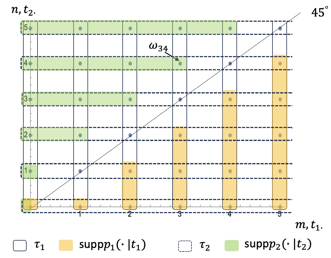
Figure 1: The information structure of the Bayesian game

The information structure of the Bayesian game is shown in Figure 1, where each point is an element in $\Omega$ (for example, the point having $3$ with respect to $t_{1}$-axis and $4$ to $t_{2}$-axis represents $\omega_{34}$) and the vertical (horizontal) slots indicate $\tau_{1}$ ($\tau_{2}$). One can see that a profile $(\theta_{1m},\alpha_{1};\theta_{2n},\alpha_{2})$ satisfies $\alpha_{1}=\Psi_{\theta_{1}m,\Delta^{\kappa}}^{\infty}$ and $\alpha_{2}=\Psi_{\theta_{2}n,\Delta^{\kappa}}^{\infty}$ if and only if it is generated from a mixed-action Bayesian equilibrium $(\sigma_{1},\sigma_{2})$ of the above Bayesian game; especially, when $|\alpha_{i}|>1$, $\sigma_{i}$ is a uniform distribution over $\alpha_{i}$.

For example, in Example 2.1, the state of the world could be $\omega_{5,7}$, which means that player 1 is level-$5$ and player 2 is level-$7$ and both chooses $0$, which forms an equilibrium, even the real level of player 2 is not in the support of player 1’s belief.

3 $\Delta^{\kappa}$-rationalizability in dynamic games and DCH solution

To extend our discussion into the dynamic situation, we study multistage games with perfect information, which is mostly used in the experimental literature. Still, we focus on 2-person games. A multistage game is a tuple $\Gamma=\langle I,(A_{j},\mathcal{A}_{j},v_{j})_{j\in I}\rangle$, where,

• $A_{i}$ is the set of potentially feasible actions for each $i\in I$,

• Let $A=\times_{j\in I}A_{j}$ and $A^{<\mathbb{N}_{0}}=\cup_{k\in\mathbb{N}_{0}}A^{k}$ be the set of finite sequences of action profiles; for each $i\in I$, $\mathcal{A}_{i}:A^{<\mathbb{N}_{0}}\rightrightarrows A_{i}$ is a feasibility correspondence that assigns each sequence of action profiles (i.e., history) $h=(a^{t})_{t=1}^{\ell}$ actions available to each player; the game terminates when $\mathcal{A}_{i}(h)=\emptyset$ for each $i$,

• For each terminal history $h$ (i.e, $\mathcal{A}_{i}(h)=\emptyset$ for each $i$), $v_{i}(h)$ is the payoff of $i$.

We use $\overline{\mathcal{H}}$ to denote the set of all feasible histories, $\mathcal{Z}$ the set of terminal histories, and $\mathcal{H}$ the set of all non-terminal histories. $\overline{\mathcal{H}}$ is naturally endowed with the prefix order. The symbol $\emptyset$ is used to denote the initial history (i.e., the beginning) of the game. At each non-terminal history $h$, a player $i$ is called active iff she has multiple available actions, i.e., $|\mathcal{A}_{i}(h)|>1$. $\Gamma$ is a game with perfect information iff at each $h\in\mathcal{H}$ only one player is active. A strategy for player $i$ is a function $s_{i}:\mathcal{H}\rightarrow A_{i}$ such that for each $h\in\mathcal{H}$, $s_{i}(h)\in\mathcal{A}_{i}(h)$. We let $S_{i}$ be the set of player $i$’s strategies and $S=S_{1}\times S_{2}$. We define $\zeta:S\rightarrow\mathcal{Z}$ to be the path function associating each strategy profile with the terminal history it generates; based on this, we can define the payoff for each player given a strategy profile by letting $V_{i}(s)=v_{i}(\zeta(s))$ for each $i\in I$ and $s\in S$. For each $h\in\mathcal{H}$, we define $S(h)$ to be the set of strategy profiles that leads to $h$, $S_{i}(h):=\operatorname{proj}_{i}S(h)$, and $S_{-i}(h):=\operatorname{proj}_{-i}S(h)$. One can see that when there is only one stage (and consequently everyone moves simultaneously at the beginning), a strategy degenerates into an action, and $\Gamma$ is equivalent to a static game.

As in Section 2, given $\Gamma$, we can define a multistage game with payoff uncertainty $\hat{\Gamma}=\langle I,(\Theta_{j},A_{j},\mathcal{A}_{j},u_{j})_{j\in I}\rangle$, where for each $i\in I$, $\Theta_{i}=\{\theta_{ik}:k\in\mathbb{N}_{0}\}$ is the set of information types, and for each $\theta=(\theta_{i},\theta_{-i})$ and $h\in\mathcal{Z}$, $u_{i}(\theta,h)=0$ if $\theta_{i}=\theta_{i0}$ and $u_{i}(\theta,h)=v_{i}(h)$ otherwise; in addition, for each $s\in S$, we define $U_{i}(\theta,s)=u_{i}(\theta,\zeta(s))$.

To describe players’ beliefs in a dynamic situation, we need a more sophisticated tool, because, as the game unfolds, players have to update and revise their beliefs based on their observations. A conditional probability system (CPS) for player $i$ is a collection $\mu^{i}=(\mu^{i}(\cdot|h))_{h\in\mathcal{H}}\in\prod_{h\in\mathcal{H}}\Delta(\Theta_{-i}\times S_{-i}(h))$ such that for all $\overline{\theta}_{-i}\in\Theta_{-i}$, $\overline{s}_{-i}\in S_{-i}$, $h^{\prime},h^{\prime\prime}\in\mathcal{H}$ with $h^{\prime}\prec h^{\prime\prime}$,

$$\mu^{i}(\overline{\theta}_{-i},\overline{s}_{-i}|h^{\prime})=\mu^{i}(\overline{\theta}_{-i},\overline{s}_{-i}|h^{\prime\prime})\left(\sum_{\theta_{-i}\in\Theta_{-i},s_{-i}\in S_{-i}(h^{\prime\prime})}\mu^{i}(\theta_{-i},s_{-i}|h^{\prime})\right)$$ (1)

In words, a CPS of a player assigns to each non-terminal history a belief about her opponent’s types and strategies, which satisfies the chain rule in (1). The set of CPSs for player $i$ is denoted by $\Delta^{\mathcal{H}}(\Theta_{-i}\times S_{-i})$. A strategy $s_{i}\in S_{i}$ is sequentially rational for type $\theta_{i}$ with respect to CPS $\mu^{i}\in\Delta^{\mathcal{H}}(\Theta_{-i}\times S_{-i})$ iff for all $h\in\mathcal{H}$ with $s_{i}\in S_{i}(h)$,

$$\mathbb{E}_{\mu^{i}(\cdot|h)}U_{i}(\theta_{i},s_{i},\cdot)\geq\mathbb{E}_{\mu^{i}(\cdot|h)}U_{i}(\theta_{i},s^{\prime}_{i},\cdot)\text{ for all }s_{i}^{\prime}\in S_{i}(h)$$

That is, $s_{i}$ is a best response for $\theta_{i}$ at each history that consistent with it. We use $r_{i}(\hat{\theta}_{i},\mu^{i})$ to denote the set of all strategies sequentially rational for $\hat{\theta}_{i}$ for $\mu^{i}$.

We extend K1-K3 in Section 2 to define the restriction $\Delta^{\kappa}$ here. One intuitive way is as follows: for each $i\in I$, $\theta_{i}\in\Theta_{i}$, and $\mu^{i}\in\Delta^{\theta_{ik}}$,

1. At each $h\in\mathcal{H}$, $\operatorname{supp}\operatorname{marg}_{\Theta_{-i}}\mu^{i}(\cdot|h)\subseteq\{\theta_{-i,0},\theta_{-i,1},...,\theta_{-i,k-1}\}$,

2. At each $h\in\mathcal{H}$, if $\mu^{i}(\theta_{-i,0}|h)>0$, $\mu^{i}(s_{-i}|h,\theta_{-i,0})=\frac{1}{|S_{-i}(h)|}$ for each $s_{-i}\in S_{-i}(h)$.

3. For each $t=0,...,k-1$, $\mu^{i}(\theta_{-i,t}|\emptyset)=f^{k}(t)$.

We still preserve the name $\Delta^{\kappa}$ since in the degenerate case (that is, $\Gamma$ is in fact a static game), condition DK$n$ coincides with K$n$ for each $n=1,2,3$; in this sense, as we mentioned before, K1–K3 are DK1 – DK3 in special cases. Note that DK2 can be equivalently rephrased in a behavioral way: at each history $h\in\mathcal{H}$, if $\theta_{-i,0}$ is deemed possible (i.e., with positive probability), then under $\theta_{-i,0}$ each action in $\mathcal{A}_{-i}(h)$ is deemed to appear with equal probabilities (see Battigalli [3] for a detailed discussion). However, as pointed out in Battigalli [3], even though it is frequently used in the experimental literature, in general, K2 is not equivalent to uniform distribution of reduced strategies conditional on $\theta_{-i,0}$ at each $h$. One might want to modify DK2 into RDK2, where strategy is replaced by reduced strategy; yet that might be characterized by different behavioral consequences.

Note that as long as $f(0)>0$, DK2 and DK3 imply that a player will never be surprised, that is, there is no history that she deems impossible at the beginning, because she always deems $\theta_{-i,0}$ possible and under $\theta_{-i,0}$, at each history, every action (of her opponent’s) is possible. Therefore, only the chain rule in (1) matters; it does not matter which notion of belief system is adopted (forward consistent, standard, or complete consistent; see Battigalli, Catonini, and Manili [6]).

Now we go to the epistemic foundation. In dynamic situations, rationality means sequential rationality. There are several ways to extend the concept of belief in some event (e.g., rationality), all of which agree on belief in that event at the beginning of the game; the problem is how to revise one’s initial belief when it is rejected by observation. By incorporating a forward-induction criterion, i.e., maintaining the belief of the event at all history that is consistent with the event, Battigalli and Siniscalchi’s [7] formulate the cornerstone concept called strong belief which is later incorporated into the framework of Battigalli and Siniscalchi’s [8] $\Delta$-rationalizability. Here, by applying Battigalli and Siniscalchi’s [8] argument, the behavioral consequences of rationality (R), common strong belief in rationality (CSBR), and transparency of $\Delta^{\kappa}$ (TCK) are characterized by the iterative procedure defined as follows.

Definition 3.10.

Consider the following procedure, called $\Delta^{\kappa}$-rationalization procedure:

Step 0. For each $i\in I$, $\Sigma_{i,\Delta^{\kappa}}^{0}=\Theta_{i}\times S_{i}$,

Step $n+1$. For each $i=1,2$ and each $(\theta_{i},s_{i})\in\Theta_{i}\times S_{i}$ with $(\theta_{i},s_{i})\in\Sigma_{i,\Delta^{\kappa}}^{n}$, $(\theta_{i},s_{i})\in\Sigma_{i,\Delta^{\kappa}}^{n+1}$ iff the there is some CPS $\mu^{i}\in\Delta^{\theta_{i}}$ such that

1. $s_{i}\in r_{i}(\theta_{i},\mu^{i})$;

2. for each $h\in\mathcal{H}$, if $\sum_{-i,\Delta^{\kappa}}^{n-1}\cap[\Theta_{-i}\times S_{-i}(h)]\neq\emptyset$, then $\mu^{i}(\sum_{-i,\Delta^{\kappa}}^{n-1}|h)=1$.

Finally, let $\Sigma_{i,\Delta^{\kappa}}^{\infty}=\cap_{n\geq 0}\Sigma_{i,\Delta^{\kappa}}^{n}$ for $i=1,2$. The elements in $\Sigma_{i,\Delta^{\kappa}}^{\infty}$ are said to be $\Delta^{\kappa}$-rationalizable.

One can see that when $\Gamma$ is degenerate, Definitions 3.10 and 2.2 coincide.

Example 3.11.

Consider the game in Figure 2 (Lin and Palfrey [21]). Suppose that $f=\operatorname{Poisson}(1.5)$.

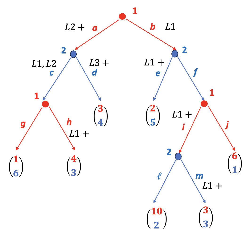
Figure 2: Palfrey and Line’s Example 4.2.1, p.15

Starting from step 1. Consider $\theta_{11}$, i.e., a level-1 player 1. Note that $\mu^{1}\in\Delta^{\theta_{11}}$ and $\mu^{1}(\Sigma_{2,\Delta^{\kappa}}^{0}|\emptyset)=1$ if and only if $\mu^{1}((\theta_{20},s_{2})|\emptyset)=\frac{1}{8}$ for each $s_{2}\in S_{2}$. Only two strategies of player 1, b.g.i and b.h.i, are optimal to the initial belief. To see which one is sequentially rational, we only need to check the choice at history $(ac)$, where one can see easily that $g$ is dominated by $h$. Hence $\Sigma_{1,\Delta^{\kappa}}^{1}(\theta_{11})=\{$b.h.i$\}$. In a similar manner we can see that, for a level-1 player 2, $\Sigma_{2,\Delta^{\kappa}}^{1}(\theta_{21})=\{$c.e.m$\}$.

Note that some strategies could also be deleted under $\theta_{i2}$ (or types with higher sophistication) at step 1. For example, it is easy to see that for each $s_{1}\in S_{1}$ with $s_{1}(ac)=g$, $(\theta_{12},s_{1})\not\in\Sigma_{1,\Delta^{\kappa}}^{1}$.

For step 2, we consider $\theta_{12}$. Now for each $\mu^{1}\in\Delta^{\theta_{12}}$, at the beginning of the game it has to satisfy $\operatorname{supp}\mu^{1}(\cdot|\emptyset)=\left(\{\theta_{20}\}\times S_{2}\right)\cup\{(\theta_{21},c.e.m)\}$, $\mu^{1}(\theta_{20}|\emptyset)=0.4$, $\mu^{1}(\theta_{21}|\emptyset)=0.6$, and $\mu^{1}((s_{2})|\emptyset,\theta_{20})=\frac{1}{8}$ for each $s_{2}\in S_{2}$. The best responses to such a belief are $a.g.i$ and $a.h.j$. Note that the difference for the two strategies is at the history $(bf)$. Note that $c.e.m\not\in S_{2}(bf)$, the belief of player 1 in $\Delta^{\theta_{12}}$ with $\mu^{1}(\sum_{2,\Delta^{\kappa}}^{1}|(bf))=1$ must be $\mu^{1}((\theta_{20},s_{2})|(bf))=\frac{1}{4}$ for each $s_{2}\in S_{2}(bf)$, which implies that by choosing $i$ player 1 gets expected payoff $6.5$, and by $j$ $6$. Therefore, for a level-2 player 1, $\Sigma_{1,\Delta^{\kappa}}^{2}(\theta_{12})=\{$a.h.i$\}$. In a similar manner one can see that $\Sigma_{2,\Delta^{\kappa}}^{2}(\theta_{22})=\{$c.e.m$\}=\Sigma_{2,\Delta^{\kappa}}^{1}(\theta_{21})$.

One can continue this procedure, and the outcome is summarized in Figure 2.

It can be easily seen that Proposition 1 still holds here. Further, we show that $\Delta^{\kappa}$-rationalizability generically coincides with Lin and Palfrey’s [21] DCH solution, a recent dynamic extension of CH. In this manner, we provide an epistemic foundation for DCH.

Definition 3.12.

Consider the following procedure, called the DCH-procedure:

Step 0. For each $i\in I$ and $\theta_{i}\in\Theta_{i}$, $\Lambda_{\theta_{i},\Delta^{\kappa}}^{0}=\{\theta_{i}\}\times S_{i}$,

Step $n+1$. For each $i\in I$, $\Lambda_{\theta_{ik},\Delta^{\kappa}}^{n+1}=\Lambda_{\theta_{ik},\Delta^{\kappa}}^{n}$ if $k\neq n+1$; for each $(\theta_{i,n+1},s_{i})$ with $s_{i}\in S_{i}$, $(\theta_{i,n+1},a_{i})\in\Lambda_{\theta_{i,n+1},\Delta^{\kappa}}^{n+1}$ iff there is some $\mu^{i}$ satisfying DK1 - DK3 such that

1. $s_{i}\in r^{i}(\theta_{i,n+1},\mu^{i})$,

2. $\mu^{i}$ satisfies the following conditions:

   • $\operatorname{supp}\mu^{i}(\cdot|\emptyset)=\cup_{t=0}^{n}\Lambda_{\theta_{-i,t},\Delta^{\kappa}}^{n}$,

   • For each $\theta_{-i,t}$ ($t\leq n$) and $s_{-i},s_{-i}^{\prime}\in S_{-i}$, if $(\theta_{-i,t},s_{-i}),(\theta_{-i,t},s_{-i}^{\prime})\in\Lambda_{\theta_{-i,t},\Delta^{\kappa}}^{n}$, $\mu^{i}(\theta_{-i,t},s_{-i}|\emptyset)=\mu^{i}(\theta_{-i,t},s_{-i}^{\prime}|\emptyset)$.

We let $\Lambda_{-i,\Delta^{\kappa}}^{n}:=\cup_{\theta_{-i}\in\Theta_{-i}}\Lambda_{\theta_{-i},\Delta^{\kappa}}^{n}$ and $\Lambda_{i,\Delta^{\kappa}}^{\infty}=\cap_{n\geq 0}\Lambda_{i,\Delta^{\kappa}}^{n}$ for each $i\in I$. $\Lambda_{\Delta^{\kappa}}^{\infty}:=\times_{i\in I}\Lambda_{i,\Delta^{\kappa}}^{\infty}$ is called the DCH-solution.

The following lemma shows that Definition 3.12 coincides with the original definition of Lin and Palfrey [21] (Section 3.2).

Lemma 3.13.

For each $i\in I$, $n\in\mathbb{N}_{0}$, and $h\in\mathcal{H}$, define $\Theta_{-i}^{n+1}(h)=\{\theta_{-i,t}:t\leq n,$ and there is $s_{-i}\in S_{-i}$ with $(\theta_{-i,t},s_{-i})\in\Lambda_{\theta_{-i,t},\Delta^{\kappa}}^{n}$ and $s_{-i}\in S_{-i}(h)\}$. Then the belief $\mu^{i}$ satisfies the conditions (i.e., KD1-KD3, conditions 1, 2.1, and 2.2) at step $n+1$ if and only if for each $h\in\mathcal{H}$, $\theta_{-i,t}\in\Theta_{-i}^{n+1}(h)$

• $\mu^{i}(\theta_{-i,t}|h)=\frac{f(t)}{\sum_{\theta_{-i,\ell}\in\Theta_{-i}^{n+1}(h)}f(\ell)}$,

• $\mu^{i}(s_{-i}|h)=\sum_{\theta_{-i,\ell}\in\Theta_{-i}^{n+1}(h)}\frac{\mu^{i}(\theta_{-i,t}|h)}{|\Lambda_{\theta_{-i,t},\Delta^{\kappa}}^{n}(h)|}$ for each $s_{-i}\in S_{-i}(h)$, where $\Lambda_{\theta_{-i,t},\Delta^{\kappa}}^{n}(h):=\{(\theta_{-i,t},s_{-i})\in|\Lambda_{\theta_{-i,t},\Delta^{\kappa}}^{n}:s_{-i}\in S_{-i}(h)\}$.

Proof 3.14.

The if part is straightforward. The only-if part follows from the chain rule (1) and condition 2.2.

Using Lemma 3.13, we can show the following statement in a manner similar to Theorem 2.4.

Theorem 3.15.

1. For each $i\in I$ and $k\in\mathbb{N}_{0}$, $\Lambda_{\theta_{ik},\Delta^{\kappa}}^{k}\subseteq\Sigma_{\theta_{ik},\Delta^{\kappa}}^{k}$; consequently, $\Lambda_{i,\Delta^{\kappa}}^{\infty}\subseteq\Sigma_{i,\Delta^{\kappa}}^{\infty}$.

2. For generic multistage games, for each $i\in I$ and $k\in\mathbb{N}_{0}$, $\Lambda_{\theta_{ik},\Delta^{\kappa}}^{k}=\Sigma_{\theta_{ik},\Delta^{\kappa}}^{k}$; consequently, $\Lambda_{i,\Delta^{\kappa}}^{\infty}=\Sigma_{i,\Delta^{\kappa}}^{\infty}$.

References

- [1] Alaoui, L., Penta, A., 2016. Endogenous depth of reasoning. Review of Economic Studies 83,1297-1333.
- [2] Aumann R. 1976. Agreeing to disagree. The Annals of Statistics 4: 1236-1239.
- [3] Battigalli P. 2023. A note on reduced strategies and cognitive hierarchies in the extensive and normal form. IGIER working paper No. 706.
- [4] Battigalli, P., Bonanno, G., 1999. Recent results on belief, knowledge and the epistemic foundation of game theory. Research in Economics 53, 149-225.
- [5] Battigalli P, Catonini E, De Vito N. 2023. Game Theory: Analysis of Strategic Thinking. Manuscript. Bocconi University. Downloadable at https://didattica.unibocconi.it/mypage/upload/48808_20230906_024712_05.09.2023TEXTBOOOKGT-AST_PRINT_COMPRESSED.PDF
- [6] Battigalli P, Catonini E, Manili J. 2023. Belief change, rationality, and strategic reasoning in sequential games. Games and Economic Behavior 142: 527-551.
- [7] Battigalli P, Siniscalchi M. 2002. Strong belief and forward induction reasoning. Journal of Economic Theory 106: 356-391.
- [8] Battigalli, P., Siniscalchi, M., 2003. Rationalization and incomplete information. Advances in Theoretical Economics 3, Article 3.
- [9] Camerer CF, Ho TH, Chong JK. 2004. A cognitive hierarchy model of games. The Quarterly Journal of Economics 119: 861-898.
- [10] Chong J-K, Camerer CF, Ho TH. 2005. Cognitive hierarchy: a limited thinking theory in games. Chapter 9 in Experimental Business Research III, ed. by Zwick R and Rapoport A, 203-228. Springer.
- [11] Dekel, E., Siniscalchi, M., 2015. Epistemic game theory. In: Young, P.H., Zamir, S., eds, Handbooks of game theory with economic applications, vol 4. Elsevier, Amsterdam, 619–702
- [12] Friedenberg, A., Kets, W., Kneeland, T., 2021. Is bounded reasoning about rationality driven by limited ability? Working paper.
- [13] Ho TH, Su X. 2013. A dynamic level- model in sequential games. Management Science 59: 452-469.
- [14] Ho TH, Park S-E, Su X. 2021. A Bayesian level- model in -person games. Management Science 67: 1622-1638.
- [15] Jin Y. 2021. Does level- behavior imply level- behavior imply level- thinking? Experimental Economics 24: 330-353.
- [16] Kaneko M, Suzuki N-Y. 2003. Epistemic models of shallow depths and decision making in games: Horticulture. Journal of Symbolic Logic 68: 163-186.
- [17] Kneeland, T., 2015. Identifying higher-order rationality. Econometrica 83, 2065-2079.
- [18] Kneeland, T., 2016. Coordination under limited depth of reasoning. Games and Economic Behavior 96, 49-64.
- [19] Koriyama Y, Ozkes A. 2021. Inclusive Cognitive Hierarchy. Journal of Economic Behavior and Organization 186, 458–480.
- [20] Levin D, Zhang L. 2022. Bridging level- to Nash equilibrium. The Review of Economics and Statistics 104: 1329-1340.
- [21] Lin P-H, Palfrey TR. Cognitive hierarchies for games in extensive form. Working paper.
- [22] Liu S., Maccheroni F. 2023. Quantal response equilibrium and rationalizability: Inside the blackbox. Forthcoming in Games and Economic Behavior.
- [23] Maschler M, Solan E, Zamir S. 2020. Game Theory, 2nd ed. Cambridge University Press.
- [24] Pearce, D. 1984. Rationalizable strategic behavior and the problem of perfection. Econometrica 52: 1029-1050.
- [25] Rubinstein A. 2007. Instinctive and cognitive reasoning: A study of response times. Economic Journal 117: 1243-1259.
- [26] Rubinstein A, Wolinstky A. 1994. Rationalizable conjectural equilibrium: between Nash and equilibrium. Games and Economic Behavior 6: 299-311.
- [27] Schipper BC, Zhou H. 2024. Level- thinking in extensive form. Forthcoming in Economic Theory.
- [28] Stahl DO. Evolution of Smartn players. Games and Economic Behavior 5: 604-617.
- [29] Stahl DO, Wilson PW. 1995. On players’ models of other players: theory and experimental evidence. Games and Economic Behavior 10: 218-254.
- [30] Strzalecki T. 2014. Depth of reasoning and higher order beliefs. Journal of Economic Behavior and Organization 108, 108–122.