X-Diffusion: Generating Detailed 3D MRI Volumes From a Single Image Using Cross-Sectional Diffusion Models

Abstract

In this work, we present X-Diffusion, a cross-sectional diffusion model tailored for Magnetic Resonance Imaging (MRI) data. X-Diffusion is capable of generating the entire MRI volume from just a single MRI slice or optionally from few multiple slices, setting new benchmarks in the precision of synthesized MRIs from extremely sparse observations. The uniqueness lies in the novel view-conditional training and inference of X-Diffusion on MRI volumes, allowing for generalized MRI learning. Our evaluations span both brain tumour MRIs from the BRATS dataset and full-body MRIs from the UK Biobank dataset. Utilizing the paired pre-registered Dual-energy X-ray Absorptiometry (DXA) and MRI modalities in the UK Biobank dataset, X-Diffusion is able to generate detailed 3D MRI volume from a single full-body DXA. Remarkably, the resultant MRIs not only stand out in precision on unseen examples (surpassing state-of-the-art results by large margins) but also flawlessly retain essential features of the original MRI, including tumour profiles, spine curvature, brain volume, and beyond. Furthermore, the trained X-Diffusion model on the MRI datasets attains a generalization capacity out-of-domain (e.g. generating knee MRIs even though it is trained on brains). The code is available on the project website https://emmanuelleb985.github.io/XDiffusion/.

1 Introduction

Medical imaging stands as a cornerstone in modern healthcare, its innovations playing a critical role in disease diagnosis and treatment planning. Traditional MRI scans, though detailed, are often time-consuming and come with significant economic implications [8]. The urgency to tackle these impediments has propelled research endeavors in the past, but the quest for a cost-efficient, rapid, and precise alternative persists[74, 3, 60]. A rapid and affordable MRI process would catalyze early disease detection, potentially saving countless lives. Moreover, by reducing the barriers to access, we would be ensuring a more holistic healthcare approach, promptly addressing diseases before they escalate.

Figure 1: X-Diffusion. We present X-Diffusion, a method that can generate detailed and dense MRI volumes from (i) a single MRI slice, or (ii) from a single DXA scan. This is the first work that we know of in the medical imaging literature to generate MRIs that preserve key properties from extremely sparse inputs. X-Diffusion can optionally accept multiple MRI slice inputs as well for full MRI generation from few MRI slices.

Traditionally, inverse 2D or 3D fast Fourier transform (FFT) [12] on k-space data with full Cartesian sampling are used to reconstruct MR images from raw data or with the help of machine learning models [24, 72, 71, 56, 9, 68, 75]. Recent years saw a pivot towards machine learning-based frameworks such as Generative Adversarial Networks (GANs) and Convolutional Neural Networks (CNNs), harnessing the power of deep neural networks to enrich MRI reconstruction [53, 34]. However, a pervasive challenge remained: the synthesis of high-resolution MRIs from extremely limited observations (or even a single 2D image). The previous works either target compressive sensing for increasing the frequency resolution of the MRI [17, 53, 34, 19] or target increasing the slice density when a sufficient number of slices is available (e.g. more than 30) [39]. These existing gaps in the MRI reconstruction landscape underscore the significance of our X-diffusion in MRI reconstruction from an extremely small number of observations.

Recently, the use of diffusion-based models for image inverse problems has shown great success [63, 18, 35, 51, 40, 52]. This motivated our X-Diffusion to investigate learning volumes instead of images. In this light, our X-Diffusion proposes a novel architecture to allow learning on 3D volumetric data by view-dependent cross-sections. This allows for full MRI generation with unprecedented accuracy from a single MRI slice, multiple slices, or even from DXA image if paired data is available (see Figure 1). To the best of our knowledge, X-Diffusion is the first work to successfully generate detailed MRI volumes from a single DXA scan, bridging the gap between two common data modalities in medical imaging. It is important to note that the generated MRIs are not clinical replacements for true MRIs, but could provide a quick, affordable, and informative “pseudo-MRI" before conducting a full MRI examination.

Contributions: (i) We introduce X-Diffusion, a cross-sectional diffusion model that generates MRI slices conditioned on a single input MRI slice or multiple slices. The proposed X-Diffusion achieves state-of-the-art results on MRI reconstruction and super-resolution compared to recent methods on BRATS, a large public dataset of annotated MRIs for brain tumours. (ii) We adapt our X-Diffusion to leverage paired and registered full-body MRI and DXA images from UK Biobank dataset to generate full-body 3D MRI from a single DXA for the first time in the literature. (iii) We validate the generated MRIs on a wide range of tasks that ensure the generated MRIs retain important features of the original MRIs, including tumor profiles, spine curvature, brain volume, and more, without using this meta-information in the generation process. (iv) We showcase the generalization of trained X-Diffusion on different datasets (knee MRIs) illustrating the potential of X-Diffusion to be the first 3D volumetric foundation model in medical imaging.

2 Related Work

2.1 3D Understanding and Generation

Multi-View 3D Reconstruction. Multi-view 3D reconstruction predicts 3D from 2D RGB images captured from different views [23, 2]. Recently, Neural Radiance Fields (NeRF) [47, 42] marked a significant shift towards 3D radiance, enabling realistic view synthesis [73, 6]. Current research optimizes NeRF for both few-shot and one-shot settings [31, 36, 81, 25]. One important difference between these few-shot NeRF works and our X-Diffusion is that we learn the explicit 3D prior on volumes by cross-sectional conditioning while those other works rely on 2D priors to enhance the neural rendering of mostly surfaces, making them less suitable for 3D volumes.

Single-View 3D Reconstruction. Previous efforts leveraged CLIP’s capabilities [54] for tasks like 3D modeling [30, 29, 48, 80]. The seminal work of DreamFusion [51] distilled a ready-made diffusion mechanism [59] into NeRF [47, 7]. This methodology ignited a myriad of new techniques, both in converting text to 3D (e.g. [40, 15]) and transitioning visuals to 3D forms (e.g. [62, 44, 41, 69]). These frameworks were considerably improved by Zero-123  [41], explicitly conditioning on camera-views while finetuning Stable Diffusion on the large 3D CAD dataset Objaverse [20]. While Zero-123 learns to generate surface renderings of a target view given a single image, X-Diffusion learns to generate a cross-sectional slice, conditioned on the angle and depth index of the slice, allowing for dense 3D volume generation and targeting MRI medical imaging.

2.2 MRI Analysis and Reconstruction

Full-Body MRI Analysis. Most methods on automatic MRI analysis focused on developing methods for local segmentation of organs or tumours [16, 22, 77, 55]. Relatively few studies looked at whole-body scans. Most of them were developed to detect and segment the spine in tasks such as scoliosis detection[33, 32, 78, 79, 11]. We leverage the MRI analysis techniques for validating the viability of the generated MRIs for tumor, spine, and other discriminative features of interest from the medical imaging community.

MRI Reconstruction. With the recent rise of foundation models in computer vision [57, 14, 50], several attempts have shown promise in steering these models for medical imaging domain [43, 49]. However, this is mainly limited to discriminative tasks such as segmentation, classification and detection. For Medical imaging inverse problem tasks, mostly classical methods were employed for incensing the resolution of the reconstruction [58, 61], or adopt diffusion models without great leverage of image pretraining [19, 17, 39, 64]. ScoreMRI and TPDM [19, 39] make use of diffusion probabilistic model (DPM) performing conditional sampling-based inverse problem. TPDM [39] proposed to overcome the limitation of ScoreMRI being an image-to-image model and leveraged the 3D prior distribution of the data using a product of two 2D diffusion models. Although this approach enables 3D generation, it only samples from two fixed canonical planes from the 3D MRI and does not work for sparse input. On the other hand, X-Diffusion leverages the full 3D volume by sampling the brain in all directions and leverages the Stable Diffusion huge image pretraining for 3D MRI volumes from a single MRI slice or an aligned DXA image.

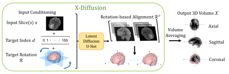
Figure 2: X-Diffusion Pipeline. A single or multi-slice input is fed into the Latent Diffusion U-Net conditioned on the target slice index $d$ and target rotation from 360^∘ slicing. The 3D volume is reconstructed by vertical stacking of the slices from a fixed axis of rotation. The final volume $\mathcal{X}$ is obtained after averaging the $N$ realigned view-dependant volumes $R_{i}^{\intercal}\mathcal{X}_{R_{i}}$ from a set of predefined target rotations $R_{i}$.

3 Methodology

In this section, we present the methodology underpinning X-Diffusion. Our approach can be delineated into three primary aspects (as shown in Figure 2):

1. Synthesizing MRI volumes using X-Diffusion models conditioned on a single MRI slice or multiple slices, with view direction and slice of volume indexing control.

2. Leveraging the multi-view capability of the X-Diffusion to aggregate multiple view-conditioned volumes to generate the final MRI output.

3. Adopting X-Diffusion to work on converting Dual X-ray Absorptiometry (DXA) to MRI volumes by utilizing a registered DXA-MRI paired dataset to create the first DXA to 3D MRI model in the medical imaging literature.

3.1 Diffusion Models Preliminaries

In previous works on view-conditional diffusion [35, 57, 41], the diffusion model $\epsilon_{\theta}$ is trained based on the objective:

$$\min_{\theta}\;\mathbb{E}_{z\sim\mathcal{E}(x),t,\epsilon\sim\mathcal{N}(0,1)}||\epsilon-\epsilon_{\theta}(z_{t},t,c(x,R,\tau))||_{2}^{2}$$ (1)

In Equation1, $\theta$ denotes the model parameters that are being optimized. The latent variable $z$ is sampled from a distribution $\mathcal{E}(x)$, where $x$ indicates the input data and $\mathcal{E}$ is a fixed encoder. $t\sim[1,2,...,T]$ specifies a particular time step during the diffusion process with maximum $T$ steps. The term $\epsilon$ is a noise variable, which is sampled from a standard normal distribution, $\mathcal{N}(0,1)$. The function $\epsilon_{\theta}$ is representative of the model’s prediction for a given $z_{t},t$, and transformation $c(x,R,\tau)$, where $R$ and $\tau$ are rotation and translation parameters, respectively.

Proceeding, the gradient of the Score Jacobian Chaining (SJC) loss, which approximates the score towards the non-noisy input as described in [41, 57], is given by: $\nabla\mathcal{L}_{SJC}=\nabla_{I_{\pi}}\log p_{\sqrt{2}\epsilon}(x_{\pi})$. The term $\nabla_{I_{\pi}}$ specifies the gradient with respect to the image $I_{\pi}$. The expression $p_{\sqrt{2}\epsilon}(x_{\pi})$ denotes the probability distribution of the transformed image $x_{\pi}$ under noise level $\sqrt{2}\epsilon$.

In our setup, $\tau$ is replaced with the index $d$ of the slice of the MRI volume and $R$ is the rotation applied on the MRI volume for the cross-sectional processing.

3.2 X-Diffusion for Cross-Sectional MRI Synthesis

Upon acquiring the MRI slice $x\in\mathbb{R}^{H\times W}$ , we seek to synthesize the entire MRI volume $\mathcal{X}\in\mathbb{R}^{H\times W\times D}$ . For this, we employ X-Diffusion $\epsilon_{\theta}$, a cross-sectional diffusion model. The fundamental idea stems from the analogy that a 3D volume can be built crosswise by stacking slices from a certain direction, just like a loaf of bread. The full target volume $\bar{\mathcal{X}}$ can be reconstructed from limited slices by generating target slices indexed by their depth $d\in[1,2,...,D]$ in the MRI volume conditioned on a certain direction $R$ where the volume is oriented. This simplifies the learning of cross-sections since the rotated MRI volume $R\mathcal{X}$ will have the same size $H\times W\times D$ as the original volume where zero padding is used. For simplicity of the processing of the data, we use the same dimensions for all directions ($H=W=D$). This allows varying the depth after rotating the ground truth MRI $\bar{\mathcal{X}}$ volume by simply indexing by the depth index $d$, and hence the slice that is used for training will be $\bar{x}_{d}=(R\mathcal{X})_{d,:,:}$. The full objective of training X-Diffusion is as follows.

$$\min_{\theta} \mathbb{E}||\epsilon-\epsilon_{\theta}(z_{t},t,c(x,d,R))||_{2}^{2}$$ (2)

s.t. $$z\sim\mathcal{E}(\bar{x_{d}}),~{}~{}t\sim[1,2,...,T]$$

$$\epsilon\sim\mathcal{N}(0,1),~{}~{}d\sim[1,2,...,D],~{}~{}R\sim SO(3)$$

The X-Diffusion model is trained with cross-sections from all different directions $R$ and all different depths $d$, which allows it to generate the target from any arbitrary rotation and depth. At inference , X-Diffusion is applied $D$ times with $d\in[1,2,..,D]$ from an arbitrary orientation $R_{i}$ to obtain the view-conditional volume $\mathcal{X}_{R_{i}}$.

$$\mathcal{X}_{R_{i}}=\begin{bmatrix}\epsilon_{\theta}(z_{t},t,c(x,1,R_{i}))\\ \vdots\\ \epsilon_{\theta}(z_{t},t,c(x,D,R_{i}))\end{bmatrix}~{}~{},~{}~{}t=1,2,...,T.$$ (3)

The volume is then rotated back by $R_{i}^{\intercal}\mathcal{X}_{R_{i}}$ to the Canonical orientation in order to proceed for validation.

Multi-slice input. While the pipeline described above is effective, it relies on heavy diffusion operations for each slice input and output. Adding more slices by simply inflating the network will create computational and memory difficulties. Therefore, to efficiently allow X-Diffusion’s pipeline to accept $K$ slices as input while maintaining the same original weights structure of Stable Diffusion [57], we perform a cumulative sum operation on the dot product of consecutive slices to reduce to a single slice input. The reduction operation of the $K>1$ input slices $(x_{1},x_{2},...,x_{K})$ is similar to what is followed in TPDM [39] in the conditioning volume, and it can be described as follows. $x=\frac{1}{K-1}\sum_{j=1}^{K}x_{j}\cdot x_{j+1}$.

Input DXA	GT d=68	Output d=68	Difference	GT d=100	Output d=100	Difference

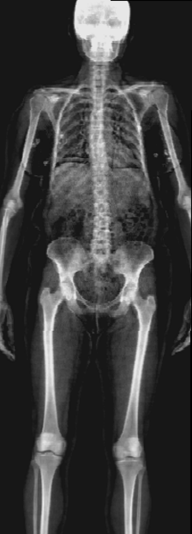
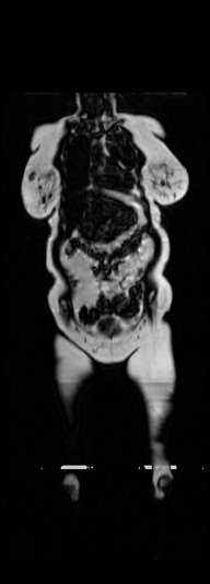
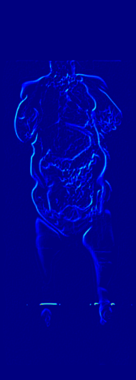
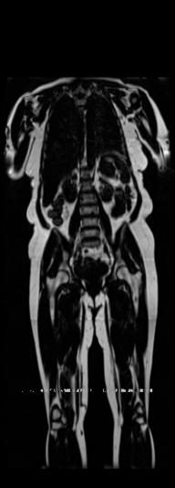
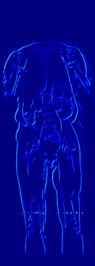
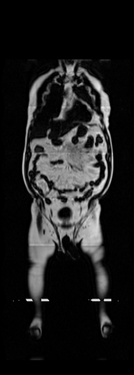
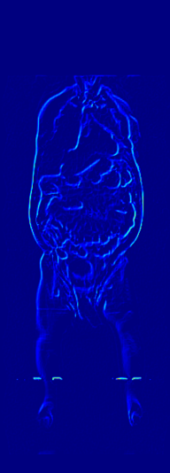
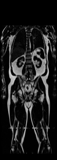
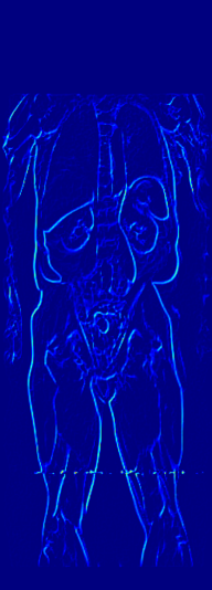
Figure 3: Qualitative Results of DXA to 3D MRI Generation with X-Diffusion. We show a single DXA example, Two corresponding ground-truth MRI slices (index 68 and 100), the corresponding generated MRI slice, and a difference map to qualitatively measure the error between generated and ground-truth MRI. Note that when stitching the MRIs in the UKBioBank dataset, there is a disparity in the bias field effect which is strongest at the knee region (brighter pixels). The same pattern is present on all samples in the dataset for a fixed depth, and hence it is learned by X-Diffusion as well.

Input	$d=57$	$d=73$	$d=77$	3D Tumour

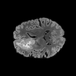
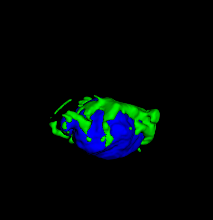
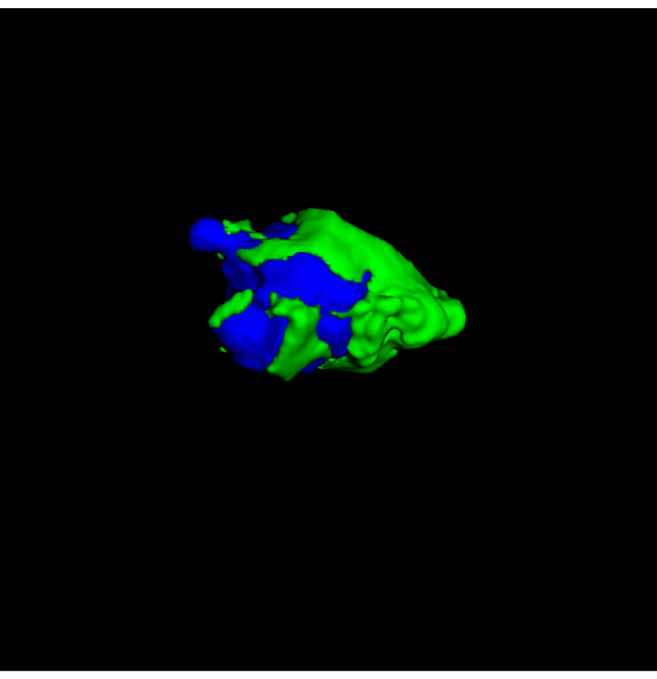
Figure 4: Visualisations of 3D Brain Generation. For the input slice (slice index 76), we show examples of slices from generated 3D brain MRI volumes with varying slice index (top) and its ground-truth brain slices (bottom). We show the tumour profile segmentation map in all output and ground truth slices to highlight the differences and show the 3D tumor in the generated MRI and ground truth MRI in the most right column. Red is used for non-enhancing and necrotic tumor core, green for the peritumoral edema, and blue for the enhancing tumor core.

3.3 Multi-View MRI Volume Generation

One advantage of our cross-sectional diffusion is that it can learn and generate the volume $\mathcal{X}_{R_{i}}$ from any arbitrary view direction $R_{i}$ (as in Equation 3). In training, this allows X-Diffusion to train on MRIs from all types of cross-sections, unlike the typically followed common 3 planes (coronal, sagittal, and axial) [19, 39, 24], which allows the model to generalize much better. At inference, we leverage this power to generate $N$ volumes from $N$ different views predefined as equally distributed views around the $360^{\circ}$ around the azimuth horizontal rotations $R_{i}\in\{R_{\text{azim}}(\frac{i\times 360^{\circ}}{N})\}_{i=1}^{N}$, where $R_{\text{azim}}(r)$ is the rotation matrix defined by rotating by $r$ degrees around the vertical axis (0,1,0). The final MRI volume output $\mathcal{X}$ is then obtained by averaging the view-conditional volumes at inference after rotating back to the canonical orientation of the output as follows.

$$\mathcal{X}=\frac{1}{N}\sum_{i=1}^{N}R_{i}^{\intercal}\mathcal{X}_{R_{i}}$$ (4)

This multi-view aggregation is inspired by how typically multi-view discriminative methods learn a global representation by average/max pooling multiple views features[66, 26, 27]. We show in Section 6.1 the utility of the volume averaging compared to a single volume.

3.4 DXA to MRI Volume Generation

DXA is a single image data modality that is similar to X-ray but includes other non-bony information such as tissue mass [67]. It measures bone mineral density and body fat composition. The radiation level is low enough that it is acceptable for conducting studies of healthy participants, such as the UK Biobank. In order to leverage X-Diffusion to synthesize the MRI volume $\mathcal{X}_{R_{i}}$ from a single DXA $u\in\mathbb{R}^{H^{\prime}\times W^{\prime}}$ (as in Figure 3), they have to be aligned, and registered. Note that, the size of the DXA does not match the MRI ($H^{\prime}\times W^{\prime}\neq H\times W$) and the scans are not registered. The two modalities in UK BioBank were not taken simultaneously but close in time hence why we believe registration is feasible for these two sequences as illustrated extensively in [79].

In order to tackle this domain gap, we leverage a registration network [79] paired with a X-Diffusion to achieve DXA to MRI slice generation. [79] introduced a multi-modal image-matching contrastive framework, that is able to learn correspondences between DXA and middle coronal MRI slices. These networks extrapolate the DXA scan by a transform $\mathbf{A}$ to the coronal MRI slice by harnessing the embedded patterns and features of the DXA and the coronal MRI mid-slice. X-Diffusion is then trained on the registered DXA ($\mathbf{A}(u)\in\mathbb{R}^{H\times W}$) and corresponding MRI slices in ($\bar{x}\in\mathbb{R}^{H\times W}$) in the target MRI volumes and is able to produce precise MRI volumes $\mathcal{X}$ that align with the DXA scans (see Figure 5 left). The other details are similar to Section 3.2 and Section 3.3.

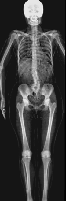
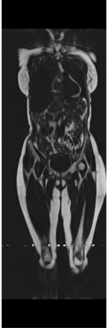
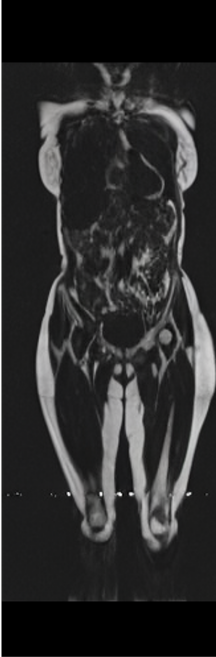
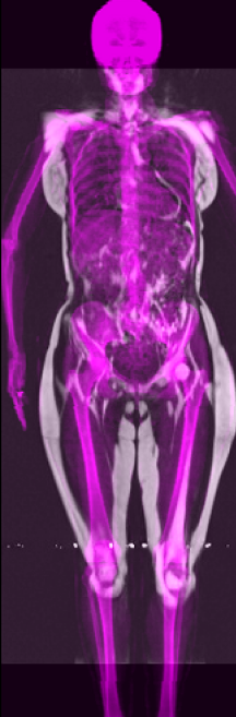
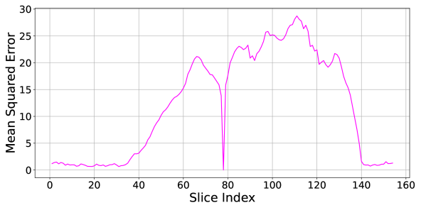
Figure 5: Alignment and Error Spread of MRI Generation. (left) We show from left to right: input DXA, ground-truth MRI, generated MRI, and overlay of the two modalities to test the alignment. The 3D PSNR for this example is 26.38 dB. (right) We show the Mean Square Error of the generated MRI from a single MRI slice (index 78) as a function of the output depth index. It shows that the error is not equally distributed in the generated MRI.

4 Experiments

4.1 Datasets

BRATS. The largest public dataset of brain tumours consisting of 5,880 MRI scans from 1,470 brain diffuse glioma patients, and corresponding annotations of tumours[4, 45, 5]. All scans were skull-stripped and resampled to 1 mm isotropic resolution. All images have a resolution of 240 $\times$ 240 $\times$ 155, and we use the flair T2 sequence. Tumours are annotated for 3 classes: Whole Tumour (WT), Tumour Core (TC), and Enhanced Tumour Core (ET).

UK Biobank. A more comprehensive dataset of 48,384 full-body MRIs from more than 500,000 volunteers[67], capturing diverse physiological attributes across a broad demographic spectrum. These Dixon MRIs do not come stitched, the scans are scanned axially and there is a disparity in the bias field effect (a common artifact of MRI machines) which is strongest at the knee region. The same knee pattern is present on all samples in the dataset. UK Biobank MRIs are resampled to be isotropic and cropped to a consistent resolution (501 $\times$ 160 $\times$ 224). 48,384 whole-body MRIs are paired with antero-posterior (AP) DXA scans of the same subjects.

IXI. A dataset of T1-weighted 1.5 Tesla brain MRI images of 582 healthy subjects, freely available online [1].

Knee fastMRI. A public dataset of raw k-space data from NYU Langone[37, 82]. We use the test set provided (n=109) of fastMRI single coil, dimensions 640x372x30. These are center-cropped to 320x320x30.

4.2 Evaluation Metrics

We use the standard 3D PSNR [39] and 2D SSIM [76] metrics to evaluate 3D MRI reconstruction and the following metrics for the validation experiments:

Dice Score. It is used to evaluate the performance of our model at segmenting the brain tumours [46]. Dice Score = $\frac{2|Y\cap\hat{Y}|}{n(|Y|+|\hat{Y}|)}$, where $Y$ is the prediction, $\hat{Y}$ is the ground-truth label and $n$ the total number of slices.

Brain Volume. We measure brain volume in $mm^{3}$ by counting the non-zero voxels in the volume multiplied by the voxel spacing [21].

Spine Curvature. Let $\gamma(t)=(x(t),y(t))$ be the equation of a twice differentiable plane curve parametrized by $t\in[0,209]$. We measure the spine curvature $\kappa$ similar to [10]: $\kappa=(y^{{}^{\prime\prime}}x^{{}^{\prime}}-x^{{}^{\prime\prime}}y^{{}^{\prime}})/(x^{{}^{\prime}2}+y^{{}^{\prime}2})^{\frac{3}{2}}$.

	Test 3D PSNR $\uparrow$
Models	1 slice		2 slices		3 slices		5 slices		10 slices		31 slices
	BR	UK	BR	UK	BR	UK	BR	UK	BR	UK	BR	UK
ScoreMRI [19]	9.37	8.54	10.25	9.16	10.68	10.42	12.37	11.88	14.31	13.24	29.24	19.01
TPDM [39]	10.48	9.29	10.86	9.99	11.33	11.09	14.13	12.62	16.65	15.88	31.48	21.70
X-Diffusion (ours)	23.1	22.42	25.2	23.04	29.43	25.26	31.25	26.85	33.27	27.44	35.48	29.01

Table 1: Model Performance on Test Brain Data and Whole-Body MRIs. We compare the MRI reconstruction for baselines ScoreMRI [19], TPDM [39] and our X-Diffusion model for varying input slice numbers in training and inference. We report the mean 3D test PSNR on BRATS (BR) brain dataset and the UK Biobank body dataset (UK). The results showcase huge improvement over the baselines, especially on the small number of input slices (particularly at 1). The parameters count and inference time of a single 3D MRI. On a single GPU a6000, 48GB of RAM for the three methods are as follows: ScoreMRI (860M, 139.1s), TPDM (1720M, 149.5s), and X-Diffusion (990M, 141.5s).

2 Slices	5 Slices	10 Slices	31 Slices	Ground Truth

Figure 6: Visual Comparison of MRI Brain Reconstruction. We benchmark different methods of reconstructed 3D brains on test set with multi-slice inputs. We show a generated slice from 3D brain generated from ScoreMRI [19] (top), TPDM[39] (middle), and X-Diffusion (bottom) conditioned on a varying number of input slices. The red zoomed crop is placed in the exact location in all images to highlight the differences.

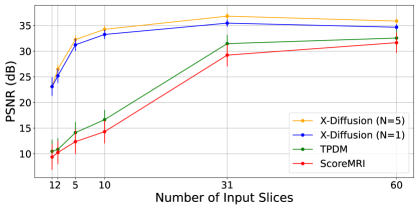
Figure 7: Effect of the Number of Input Slices. We plot the test PSNR vs. number of input slices for X-Diffusion and our baselines i.e. TPDM [39] and ScoreMRI [19] on the brain MRI dataset. $N$ is the number of averaged view-dependent volumes. We show the standard deviation of each run to account for potential randomness.

4.3 Baselines

We compare X-Diffusion’s performance against state-of-the-art MRI generation techniques, namely ScoreMRI [19] and Two-Perpendicular-Diffusion-Models TPDM [39] using ncsnpp model [65]. For the multiple slice input (nx256x256) in X-Diffusion, we aggregated the multiple inputs to form a single batch (1x256x256). For comparison with Score-MRI, being an image-to-image model, we uniformly sampled $n$ slices along the z-axis. As for TPDM, we conditioned on $n$ slices from the full volume after the fusion of the two diffusion models.

4.4 Implementation Details

To facilitate using the pretrained weights of Zero-123 [41] (based on Stable Diffusion [57]), we use the same channel size in the input 3, repeating the grayscale images. For the size of the MRI volumes, we used $H=W=D=155$, as originally the sizes in the dataset were 155 slices. For model training, we use a base learning rate of $1.0e^{-06}$, LambdaLinearScheduler with warm-up every 100 steps. Batch size is set to 32. In the diffusion sampling, we used $T=1000$ time steps and an ETA of 1.0. More details about the datasets, metrics, and setup are provided in supplementary material.

5 Results

5.1 Main Results

Our results unequivocally highlight the superior performance of X-Diffusion in terms of both qualitative and quantitative metrics. Representative MRI volumes generated by our pipeline, when juxtaposed with ground-truth images, showcased remarkable similarity, with even intricate physiological features like tumor information, spine curvature, and fat distribution being accurately captured.

Notably, X-Diffusion achieves state-of-the-art $PSNR>30$ dB for a few input slices while baselines require more than 60 input slices to achieve similar performance (Figure 7). The margin is more than 12 dB PSNR for the 1-slice input in both the BRATS and the UK Biobank benchmarks (see Table 1 and Figure 6). For reference, two randomly sampled MRIs from UK Biobank would have a PSNR of 15.95 dB $\pm$ 0.36 (on 4800 randomly sampled examples). Omitting the preprocessing step of alignment DXA to MRI, leads to a drop of PSNR on average by 2.87 dB (29.01 dB $\rightarrow$ 26.14 dB). The slices from 3D reconstructed volumes at varying depths and axis of rotation, visually match the ground truths for both brain and whole-body scans (see Figures 4 and 5 left). We also plot the error map (Figure 3) and the spread of the error (Figure 5 right) of such X-Diffusion generations to highlight the differences with the ground truth MRIs.

5.2 MRI Validation Results

Brain Volumes Preservation. The generated MRIs by our X-Diffusion retain almost the exact same average brain volume $1.28e^{6}$ $mm^{3}$ vs. $1.31e^{6}$ $mm^{3}$ of the real MRIs.

Tumour Information Preservation. For the brain tumor segmentation, we use a Swin UNETR model[28, 70], trained with random rotation, and intensity as data augmentation. On the test set with human ground-truth annotations ($n=333$), the brain volumes generated from single slice input preserve the volume of the different tumour components (paired t-test, $p-value<0.05$ for all 3 classes). In Figure 4, we highlight the tumor profiles of the generated MRIs compared to the ground truth tumour profile. The real MRI Dice score in the test set is 85.15 while the generated MRIs from a single slice have a dice score of 83.09. This shows how the generated MRIs indeed preserve the tumor information and can act as an affordable and informative pseudo-MRI, before conducting an actual costly MRI examination in hospitals. More detailed results are provided in supplementary material.

Preservation of Spine Curvature. For the spine segmentation on UK Biobank, we use a UNet++ model [83] with Dice Loss. We use a model trained to predict curves on DXA on UK Biobank [11]). We measure the Pearson correlation factor [11] of spine curvature measured on the generated MRIs where the input is a single MRI coronal slice, a single sagittal slice, or from the paired DXA, against the curvature of reference real MRIs of the same samples. The correlation coefficients are 0.89 for the coronal MRIs, 0.88 for the sagittal MRIs, and 0.87 for the DXAs on the test set of 308 human-annotated angles. We can then bin the curvature of the spines under different scoliosis categories based on human-annotated angles: mild: $0.06<\kappa<0.12$, moderate: $0.12\leq\kappa<0.15$, and severe $\kappa\geq 0.15$. We show the results in Figure 8. This illustrates that the generated MRIs preserve the spine curvature from normal to severe scoliosis cases. Additional details about spine curvature are provided in supplementary material.

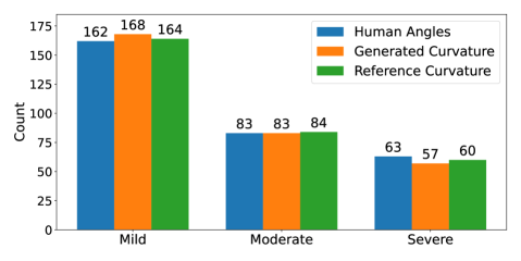
Figure 8: Scoliosis Categories of Generated MRIs. We show spine curvature predicted vs. reference curvature and human annotated angles for scoliosis categories in section 5.2. The barplot indicates that our generated MRIs maintain almost the same distribution of scoliosis categories for then set of 308 patients annotated in the UK Biobank.

5.3 Out-of-Domain Generalisation

One way to test the generalization capability of the trained X-Diffusion is to test it on a completely different domain from an MRI dataset not seen during training. We report the single-slice results on NYU fastMRI [37, 82], a knee MRI dataset, using the X-Diffusion trained on the BRATS brain MRIs. The results are shown in Figure 9 and Table 2. It shows how successfully X-Diffusion is able to generate knee MRIs from a single image, despite not seeing knees at all in training. To qualitatively assess how realistic our generated 3D volumes were (produced from a single slice), we gave 20 generated examples alongside their real MRI counterparts to an expert orthopaedic surgeon. He was then asked to identify the real example from a given pair. The surgeon identified with certainty only 10 real knee MRIs out of 17, while could not decide on the remaining 3 of the 20 MRI pairs. This further validates the generated out-of-domain MRIs.

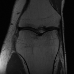
Figure 9: Out-of-Domain Generations of X-Diffusion. We show an example of knee 3D MRI generation using X-Diffusion from the single input slice on the left. We show (top): different slices of the generated 3D MRI, (bottom): ground truth slices of the same sample as reference. Our X-Diffusion can generate high-fidelity 3D MRIs of knees, even though it is trained on BRATS brain MRI dataset, illustrating its potential as a foundation model for 3D MRI generation.

6 Analysis and Ablation Study

6.1 Volume Averaging

We study the effect of volume averaging at inference as detailed in Equation 4. We note (from Figure 7) how the averaging volumes indeed increase the performance up to a certain point. The results 3D PSNR (dB) for the 31-slices X-Diffusion on $N=$ 1, 2, 3, 5, and 10 volumes are 35.48, 35.94, 36.17, 37.40, and 36.72 respectively. This is consistent with multi-view understanding literature [26].

6.2 Why does X-Diffusion Work?

The Effect of Pretraining. We hypothesize that the massive pretraining of our X-Diffusion based on Stable Diffusion weights [57] played an important role. Another aspect is that the Zero-123 [41] weights which are modified Stable Diffusion weights that understand viewpoints and fine-tuned on large 3D CAD dataset Objaverse [20] can indeed be the reason why X-Diffusion generalizes well. The PSNR for 1-slice on BRATS dataset are (SD-pretraining): 21.52 dB, (Zero-123-pretraining): 23.13 dB, (no-pretraining): 17.14 dB. These results highlight the importance of pertaining to X-Diffusion.

Leveraging Context. Since we train on a predominantly cancerous brain dataset, one question that might arise is whether X-Diffusion generated MRIs preserve tumour information when the given inputs do not intersect with any tumour. We perform experiments varying the input slice index used to generate the 3D brain MRIs and measure the performance for input slices with no intersection with the tumour (not a single pixel with tumor label in the input slice). We also measure performance when only input slices are selected from tumor range. The Dice Scores of the random slices, no-tumour, and only-tumour are 83.09, 79.23, and 83.68 respectively. As can be seen here, the brain volumes generated from input slices with no tumour still preserve tumour information in reconstructed brain volumes despite a small drop in performance. This indicates that X-Diffusion is leveraging the context to preserve key information, such as tumor locations. This observation is consistent with how tumor segmentation models with global context [13] perform better than local-based U-Nets. More details are provided in supplementary material.

	PSNR$\uparrow$	SSIM$\uparrow$
Method		Axial	Coronal	Sagittal
ScoreMRI (multi) [19]	30.88	0.82	0.82	0.81
TPDM (multi) [39]	33.76	0.87	0.86	0.87
X-Diffusion (single)	34.17	0.88	0.87	0.88
X-Diffusion (multi)	36.57	0.89	0.88	0.89

Table 2: Out-of-Domain Results. We evaluate 3D knee generation using 3D PSNR and mean SSIM on the test set of $n=109$ knees. We show a comparison between X-Diffusion and baselines that are all trained on brain MRIs from BRATS.

6.3 When does X-Diffusion Fail?

To see when and how X-Diffusion fails, we conducted an experiment on healthy brains (no tumour) using IXI dataset, by running an X-diffusion trained on BRATS brain tumor dataset. Our X-Diffusion achieved a PSNR of 35.86 dB on the IXI dataset despite being trained on the BRATS dataset. We then ran the tumour segmenter on the set of 582 healthy scans and corresponding generated MRIs. The segmenter predicted tumours in 9.9% of the real healthy brains and in 11.3% of the generated brain MRIs. Some of these tumor hallucination examples fron X-Diffusion generation are shown in Figure 10.

Hallucination	Reference	Hallucination	Reference	Failure	Reference

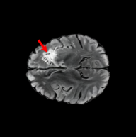
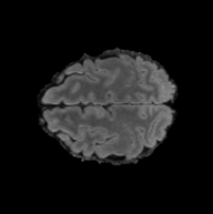
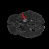
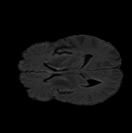
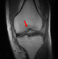
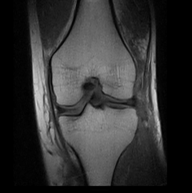
Figure 10: Tumour Hallucination and Failure Cases in X-Diffusion Generation. We show two cases of failure (red arrow) of our model hallucinating tumour in healthy sample scans. These tumour hallucinations represent only 2% of the healthy sample test set. Also, we show a failure case for the out-of-domain knee generation with the reference ground truth MRI slice.

7 Conclusions and Future Work

X-Diffusion advances 3D MRI generation, achieving high precision with limited inputs, as confirmed by tests on BRATS and UK Biobank data. Future directions include extending its application to dynamic MRI types and exploring its utility in other domains like environmental sciences.

Limitations. X-Diffusion occasionally exhibits minor artifacts in complex tissue interfaces, a known issue in generative models operating in input-sparse scenarios. An instance of this is discussed in Section 6.3 and supplementary material with additional examples.

Acknowledgement. We thank Professor Andrew Zisserman for his insightful discussions. This work was supported by the Centre for Doctoral Training in Sustainable Approaches to Biomedical Science: Responsible and Reproducible Research (SABS: R3), University of Oxford (EP/S024093/1), and by the EPSRC Programme Grant Visual AI (EP/T025872/1). We are also grateful for the support from the Novartis-BDI Collaboration for AI in Medicine. Part of the support is also coming from KAUST Ibn Rushd Postdoc Fellowship program.

Appendix A Detailed Setup

A.1 Evaluation Metrics

To quantify the efficacy of X-Diffusion, we employed a suite of evaluation metrics, namely:

• Peak Signal-to-Noise Ratio (PSNR): Indicates the quality of the reconstructed MRI by assessing the fidelity of the generated MRI in relation to the original.

  $$PSNR(x,\hat{x})=10log_{10}(\frac{max(x)^{2}}{\frac{1}{n}\sum_{i,j,k}(x_{i,j,k}-\hat{x}_{i,j,k})^{2}})$$ (5)

  where x represents the ground truth volume, $\hat{x}$ is the predicted volume, and n is the total number of voxels in the ground truth volume.

• Structural Similarity Index (SSIM): Captures the perceived changes between the original and generated MRI images.

  $$SSIM(x,\hat{x})=\frac{(2\mu_{x}\mu_{\hat{x}}+C_{1})+(2\sigma_{x{\hat{x}}}+C_{2})}{(\mu_{x}^{2}+\mu_{\hat{x}}^{2}+C_{1})(\sigma_{x}^{2}+\sigma_{\hat{x}}^{2}+C_{2})}$$ (6)

  where $x$ denotes the ground truth slice, $\hat{x}$ is the predicted slice, $\mu{x}$ is the average of $x$, $\sigma_{x}^{2}$ is the variance of $x$, $\sigma_{x\hat{x}}$ is the covariance between $x$ and $\hat{x}$, $C_{1}$=$(k_{1}L)^{2}$, $C_{2}$=$(k_{2}L)^{2}$, L is the dynamic range of pixel values, and $k_{1}$=0.01 and $k_{2}$=0.03.

  We measured the random PSNR on the whole test set for reference on the UKBiobank, BRATS, and knee fastMRI dataset. For the UKBiobank, two randomly sampled MRIs have a PSNR of 15.95 $\pm$ 0.36 dB. For BRATS, it is of 19.89 $\pm$ 1.59 dB, and for the knee fastMRI of 20.21 $\pm$ 2.58 dB.

  On BRATS dataset only

• Dice Score: We use the average Dice score to evaluate the performance of our model at segmenting the brain tumours [46]: Dice Score = $\frac{2|Y\cap\hat{Y}|}{N(|Y|+|\hat{Y}|)}$, where $Y$ is the prediction, $\hat{Y}$ is the ground-truth label and $N$ the total number of slices in the set.

• Brain Volume:
  We measure brain volume in $mm^{3}$ by counting the non-zero voxels in the volume multiplied by the volume in $mm^{3}$ of each voxel [21].

  $$NonZeroVoxCount=\sum_{i}^{N}V(x_{i},y_{i},z_{i})>0$$ (7)

  
  

  $$VoxVol(mm^{3})=v_{x}*v_{y}*v_{z}$$ (8)

  $$BrainVol=NonZeroVoxCount*VoxVol$$

  On UK Biobank dataset only

• Ground-truth Correlation Index: Pearson’s correlation coefficient $r$ measures the strength of a linear association between two variables. The formula in 9 returns a value between -1 and 1, where: 1 denotes a strong positive relationship; -1 denotes a strong negative relationship; and zero denotes no relationship [11].

  $$r=\frac{\sum_{i=1}^{n}(x_{i}-\bar{x})(y_{i}-\bar{y})}{\sqrt{\sum_{i=1}^{n}(x_{i}-\bar{x})^{2}}\sqrt{\sum_{i=1}^{n}(y_{i}-\bar{y})^{2}}}$$ (9)

• Spine Curvature Let $\gamma(t)=(x(t),y(t))$ be the equation of a twice differentiable plane curve parametrized by $t\in[0,209]$. We measure the spine curvature $\kappa$ with the standard mathematical formula [10]:
  $\kappa=(y^{{}^{\prime\prime}}x^{{}^{\prime}}-x^{{}^{\prime\prime}}y^{{}^{\prime}})/(x^{{}^{\prime}2}+y^{{}^{\prime}2})^{\frac{3}{2}}$.

A.2 Implementation Details

We conducted our experiments on two primary datasets:
BRATS. 5,880 brain MRIs annotated by expert clinicians for three classes: Whole Tumour (WT), Tumour Core (TC), and Enhanced Tumour Core (ET) [4, 45, 5]. We split the 5,880 MRIs into train (n = 4704), validation (n = 588), and test (n = 588) sets.
UKBiobank. 48,384 full-body Dixon MRIs from more than 500,000 volunteers[67]. We split the UKBiobank MRIs into train (n = 38 707), validation (n = 4839), and test (n = 4838) sets. These Dixon MRI patches could not be stitched seamlessly with our current pipeline. These artifacts appear on all scans of the UKBiobank that we stitch. Therefore, the X-Diffusion trained on this data will recreate these artifacts regardless of input. The same pattern is present on all samples in the dataset for a fixed depth, while different depth indices will have different fixed patterns. We made sure there was a coherence split, such that each patient was in a unique set. We will publish the unique IDs used for train-validation-testing to confirm there is no leakage, nor retrieval of images.

We implement X-Diffusion based on the Stable Diffusion [57] U-Net with additional controls and conditions. We detail some of the hyperparameters and design choices below.

For the first stage of autoencoder training, the encoder downsamples the image $x\in R\textsuperscript{H\texttimes W\texttimes 3}$, where $H=W=256$ by a factor $8$ to allow the DPM to focus on the semantic features of the latent space in a computationally efficient manner. KL regularization is added to mitigate high variance latent space. In the second stage, a DPM is trained on the learned lower-dimensional latent space. The configuration of the U-Net is as follows: 2 residual blocks, channels multiples: [ 1, 2, 4, 4 ], attention resolutions: [ 4, 2, 1 ], 8 heads, using spatial transformer with depth = 1. For the DDPM Latent Diffusion, we use a base learning rate of $1.0\textsuperscript{-06}$, timesteps $T=1000$, image size = 32, channels = 4, and hybrid conditioning (concatenation and cross attention). Sampling is performed with classifier free guidance (see FigureI for example of test time sampling).

We use image-conditioned stable diffusion $v2$ checkpoint from Lambda Labs. We follow the novel view synthesis training from Zero-123. X-Diffusion is trained on a single GPU a6000, 48GB of RAM for four days.

Input	$t=5$	$t=15$	$t=215$	$t=265$
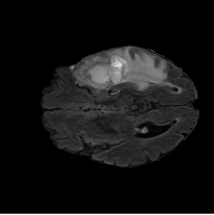
GT	$t=465$	$t=690$	$t=890$	$t=990$

Figure I: Test Time Brain Generation at Different Sampling Steps. For the input slice (top left), we show the ground-truth slice (bottom) and corresponding brain slice generating at different sampling steps $t$ in the denoising diffusion process.

Input	$d=42$	$d=48$	$d=65$	$d=69$
	7.609	9.031	8.993	8.584

Figure II: Residual Error of Generated MRIs. For the input slice (left), we show a difference map(bottom) between generated MRI (top) and ground truth. Below the (bottom) row, we indicate the mean squared error between generated and ground-truth images. Brighter pixels indicate greater disparity.

$d=97$	$d=104$	$d=108$	3D Tumour

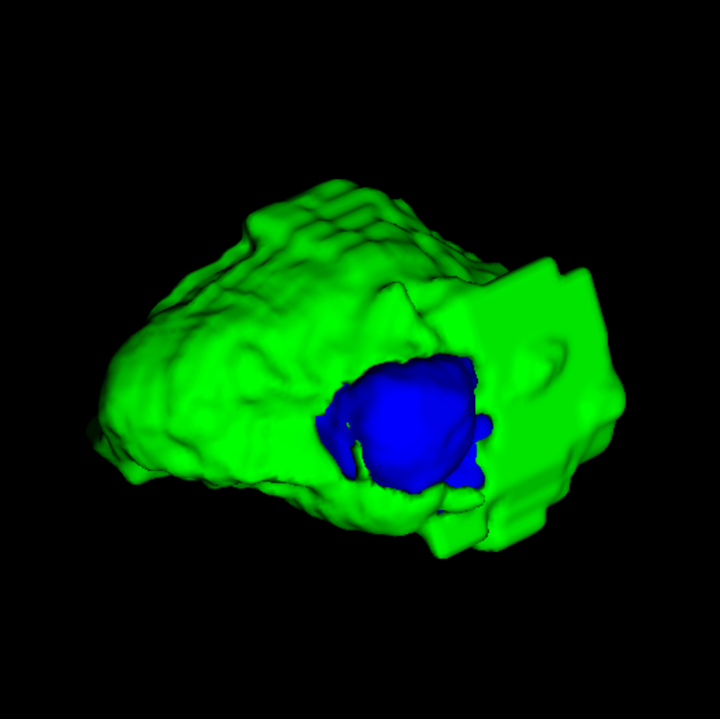
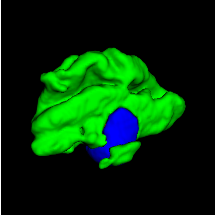
Figure III: Generated MRIs with Segmentation Maps Overlaid. We show ground-truth segmentation maps(bottom) and generated MRI (top). Red is used for the non-enhancing and necrotic tumor core, green for the peritumoral edema, and blue for the enhancing tumor core. The 3D Dice Score for this example is 77.26.

Input

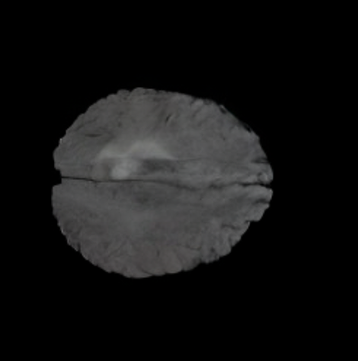
Figure IV: Probabilistic Output for Different Volumes Generated from Single Slice by X-Diffusion. For the same input slice (top left), we show 12 generated output slices ( at index $d=88$) using 12 different inputs Gaussian noise for X-Diffusion U-Net.

Input DXA	GT MRI	Generated MRI	Difference

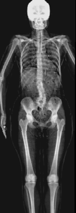
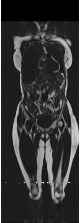
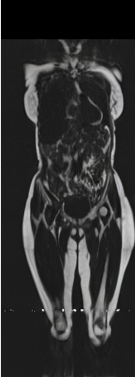
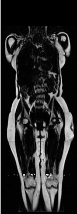
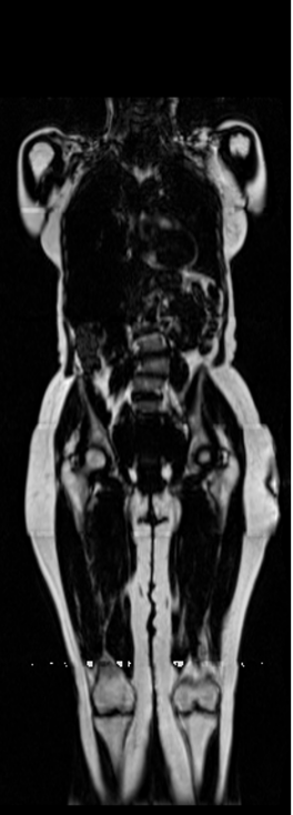
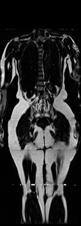
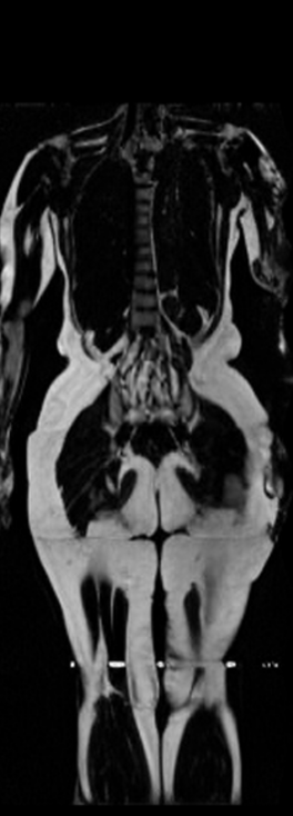
Figure V: Extension of Figure 5 from Main Paper. We show input DXA 1st column, generated MRI 2nd column, ground-truth MRI 3rd column, and Difference Map 4th column with residual value $\epsilon$.

Appendix B Additional Results

B.1 Fat Validation

We ran further experiments to investigate whether the generated MRIs (see an example in Figure V) preserve fat information. We use an image-based regression network trained on the UKBiobank to estimate DXA metadata information from 2D compressed middle coronal and sagittal MRIs [38]. Pearson’s correlations using Equation 9 comparing reference values and generated values are reported in Figure VIII with most fields having high correlation $r>0.9$. We show that the generated MRIs preserve crucial internal information.

B.2 Brain Volumes Preservation

The comparison of generated MRIs versus reference MRIs suggest a nearly perfect preservation of brain volume (in mm³) with median volume of reference MRIs of $1.31e^{6}$ $mm^{3}$ versus generated MRIs $1.28e^{6}$ $mm^{3}$ (see an example of brain generation in Figure II).

B.3 Tumour Information Preservation

On the test set with human ground-truth annotations ($n=333$), the brain volumes generated from single slice input preserve the volume of the different tumour components (paired t-test, $p-value<0.05$ for all 3 classes) (see Table I). The real MRI Dice scores are put for reference to our generated MRIs. X-Diffusion outperforms baselines TPDM [39] and ScoreMRI [19] in tumour preservation (see Table I and Figure III). We ran experiments comparing the tumour segmentation Dice Score varying X-Diffusion configurations. The multi-slice input X-Diffusion achieves marginally better Dice Score than the single slice input model (83.47 $\rightarrow$ 83.09). We also ran experiments with slice input used for volume reconstruction intersecting or not with tumour. We observe on average a drop of 6% Dice Score (see Table I). Further away from the tumour the input slice for volume reconstruction is selected, we observe a linear decrease in tumour segmentation Dice Score with lowest value of 77.21 Dice Score (see Figure VI).

This shows how the generated MRIs indeed preserve the tumour information and can act as an affordable and informative pseudo-MRI, before conducting an actual costly MRI examination in hospitals. Given that our model has been trained on brain scans all with tumours, we expect to see hallucinations of tumours in healthy scans. We report two cases of failure of our model in Figure VII. Hallucinations of tumours on healthy samples represent 2% of the test set.

	Test Dice Score $\uparrow$
X-Diffusion Generated MRIs	ET	WT	TC	Average Dice	3D PSNR(dB)$\uparrow$
single slice	75.48	89.24	84.57	83.09	35.81
multi-slice	75.82	89.56	85.04	83.47	36.13
multi-slice (only-tumour)	76.12	90.04	85.87	84.01	36.98
multi-slice (no-tumour)	70.14	84.29	81.65	78.69	33.24
Real	76.47	91.13	86.24	85.15	N/A

Table I: Dice Score for Brain Tumour Segmentation on Real vs. Reconstructed MRIs with our X-Diffusion. We show Dice Score for generated MRIs ($n=587$) by our X-Diffusion when input only intersection with tumour (only-tumour) and when input does not intersect with tumour (no-tumour) for single slice and multi-slice input (31 slices). Note how X-Diffusion predicts the correct 3D tumour locations even when the input 2D slice does not intersect the tumour in most cases (drop from 83.47 to 81.65 Dice Score).

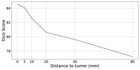
Figure VI: Dice Score versus Distance to Tumour. We show the decrease in Dice Score for slice selection at increasing distance from the centre ($0mm$) of the tumour up to $80mm$ (where slice index $\in[1,5]\cup[151,155]$, total number of slices is 155 per scan, $n=587$).

Failure	Reference	Failure	Reference

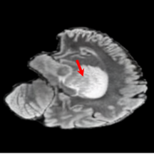
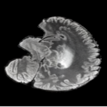
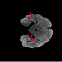
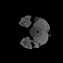
Figure VII: X-Diffusion Failure Cases. We show two cases of failure (red arrow) on BRATS generations.

B.4 Preservation of Spine Curvature and Fat

For the spine segmentation on UK Biobank, we use a UNet++ model [83] with Dice Loss. We use a model trained to predict curves on DXA on UK Biobank [11]. We show in Figure IX that generated MRIs preserve the spine curvature from normal to severe scoliosis cases. We also study the case when DXA is used to generate the MRIs and show in Figure IX how the correlation to real curvatures compares to the input MRI case. The curvatures of the MRI generated from the coronal plane match the DXA curvatures more than the curvatures generated from sagittal MRI. This is expected since the antero-posterior plane of DXA is equivalent to the coronal plane for MRIs. This also explains the greater Pearson’s correlation coefficient $r$ of the coronal MRI (0.89) and DXA-generated curvature (0.88) compared to sagittal-generated curvature (0.87) relative to the reference curvature on the coronal plane. We observe though that MRI generation using X-Diffusion from another plane than the conventional plane for scoliosis assessment is valid.

	Test 3D PSNR $\uparrow$
Input Slices	1 slice	2 slices	3	5	10	31	60	120
X-Diffusion	22.30	23.50	24.63	25.77	26.79	25.55	24.44	24.24

Table II: Model Performance on Synthetic Cone Data. We report the test 3D PSNR on synthetic volume generation of our model X-Diffusion for varying input slice number in training.

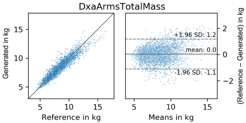
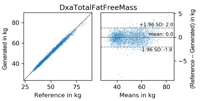
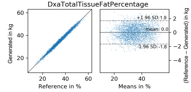
Figure VIII: Evaluation of Fat Estimation for Reference versus Generated MRIs. We show correlation (left) and mean difference plot (right) for DxaArmsTotalMass (top) with $r$ < 0.95, and DxaTotalFreeMass (middle), and DxaTotalTissueFatPercentage (bottom) with $r$ > 0.95 from Table .

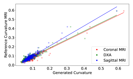
Figure IX: Curvature Preservation of Generated MRIs. We plot spine curvature measured on reconstructed MRIs where the input was either, (i) a single MRI coronal slice, (ii) a single sagittal slice, or (iii) from the paired DXA, against the curvature of reference real MRIs of the same samples. The correlation coefficients are 0.89 for the MRIs, 0.88 for the MRIs from sagittal plane generation, and 0.87 for the DXAs.

Appendix C Additional Analysis

C.1 Ablation Study

Repeated Input Single Slice in Multi-Slice Models. We try to see whether the multi-slice models are better than single slice models by studying if we used repeated input single slice multiple times. The 3D PSNR results for multi-slice input with 1, 2, 3, 5, 10, 31, and 60 repeated slices are 23.1, 23.256, 23.638, 23.921, 24.379, 25.125, and 24.921 respectively.

The Effect of Pretraining. We hypothesize that the massive pretraining of our X-Diffusion based on Stable Diffusion weights [57] played an important role. Another aspect is that the Zero-123 [41] weights which are modified Stable Diffusion weights that understand viewpoints and fine tuned on large 3D CAD dataset Objaverse [20] can indeed be the reason why X-Diffusion generalizes well to out-of-domain dataset (see generalization to knee MRIs in Figure XI).

We show the results in the following Table III.

	3D PSNR$\uparrow$
Models	1 slice	2 slices	3 slices	5 slices	10 slices	31 slices	60 slices
X-Diffusion (pre-training)	23.13	25.25	29.43	31.25	33.27	35.48	33.18
X-Diffusion (no-pretraining)	21.52	23.42	25.16	27.06	29.32	27.86	27.43

Table III: X-Diffusion with Pre-Training versus no Pre-Training. We show comparison of X-Diffusion with fine-tuning pre-trained Stable Diffusion weights versus no pre-training.

Different Mechanisms for Multi-Volume Aggregation. We used view-dependant volume averaging as described in the main paper in all of the main results in the work. We show probabilistic outputs in Figure IV for different brain volumes generated for a single slice. We show the results of varying the number of volumes in Figure X. We see that as the number of volumes averaged increase, the performance increase up to a certain point before saturating (as noted in the multi-view literature [26]). We did try to use other ways to aggregate the view-dependant volumes (e.g. by max pooling the volumes) and show the results as follows in Table VII.

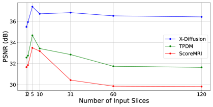
Figure X: Effect of the Number of Volume Averaged. We plot the test PSNR vs. number of volume averaged for X-Diffusion and our baselines i.e. TPDM and ScoreMRI for 31-slice mode on BRATS dataset. The PSNR increases up to 5 volumes averaged before dropping and stabilising at 60 volumes averaged for X-Diffusion and baselines.

MRI Volumes Specificity. One hypothesis that can justify why the X-Diffusion model works very well on MRIs is that MRI data is not ordinary volume data since it is obtained by actually running an inverse Fourier transform on different k-frequency components, which means that the 3D information is embedded in every slice of the MRI. Introducing this Fourier effect on our synthetic Cone volumes dataset by applying masks on the high frequencies and then inverse Fourier results in slight improvement of volume reconstruction of $+0.51$ PSNR (dB) higher than with no Fourier masking ($26.788\rightarrow 27.298$ dB). This indicates that the Fourier frequency effect is negligble and does not explain away the performance of X-Diffusion.

C.2 Time and Memory Requirements

Lowering reconstruction speed is important for greater accessibility, MRI re-acquisition purposes, and to monitor surgery in the case of dynamic MRI. The number of model parameters should be kept low to enable implementation on machines with lower memory capacity. X-Diffusion is in par with other diffusion based baseline models, albeit higher in memory requirements than classical methods. However, X-Diffusion is the only 3D medical imaging diffusion model that shows the capacity to generalize beyond the training data, opening the potential for foundation models in 3D MRIs. We show the cost analysis in Table V.

	Test 3D PSNR $\uparrow$
Models	1 vol	2 vol	3 vol	5 vol	10 vol	20 vol	31 vol	60 vol
ScoreMRI [19]	31.67	31.86	32.23	33.49	33.19	32.16	30.43	29.86
TPDM [39]	32.57	32.76	33.25	34.68	33.43	32.93	32.85	31.75
X-Diffusion (max-pool)	35.48	35.48	35.52	35.48	35.31	35.46	35.19	35.33
X-Diffusion (averaging)	35.48	35.94	36.17	37.40	36.72	36.35	36.83	36.53

Table IV: Effect of Volume Averaging on The Performance. We show best performing model on BRATS with number of volumes averaged from view-dependent 3D MRI generation. We see that the PSNR reaches a peak for 5 volumes averaged before stabilising at 10 volumes.

Models	#Params	Runtime (s)
Score-MRI[19]	860M	139.142
TDPM[39]	1720M	149.468
X-Diffusion	990M	141.461

Table V: Cost Analysis. We show compute cost and runtimes that are measured on a computer with a single GPU a6000, 48GB of RAM.

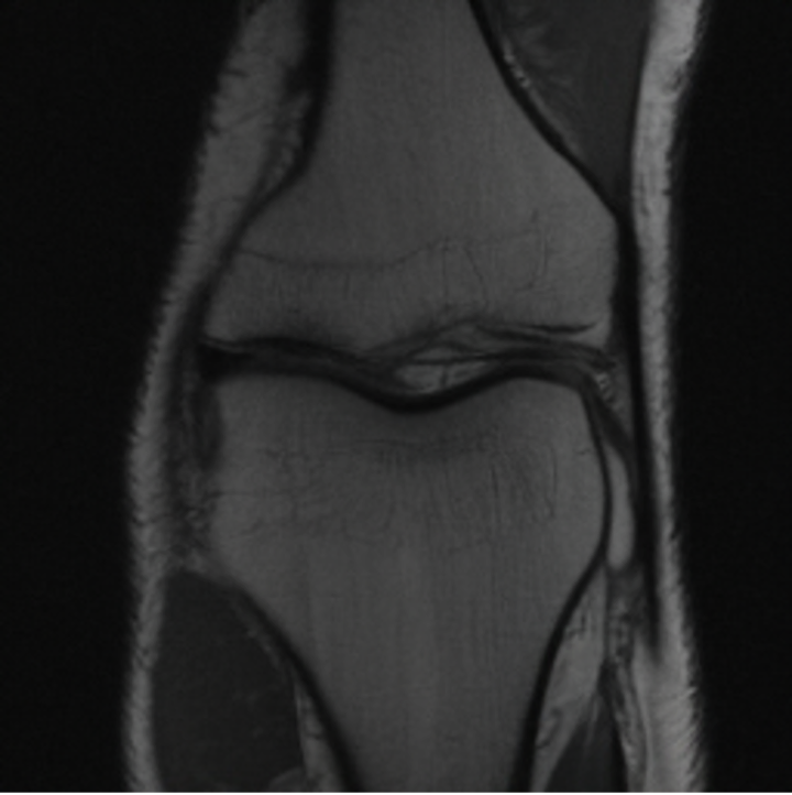
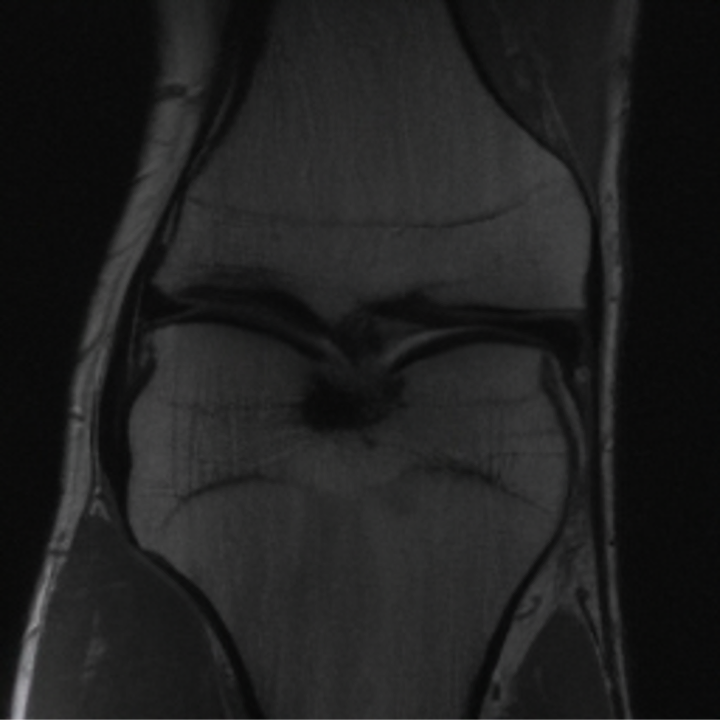
Figure XI: Out-of-Domain Knee Generations of X-Diffusion 1. We show two examples of knee 3D MRI generation using X-Diffusion from the single input slice on the left. We show (top): different slices of the generated 3D MRI, (bottom): ground truth slices of the same sample as reference. Mean PSNR for top example is of 36.84 dB and for bottom example of 35.17 dB.

C.3 Compressed Sensing Experiment

Some of the previous works on MRI reconstruction [17, 19] target the task of compressive sensing, where the goal is to increase the frequency resolution of the MRIs when the k-space is undersampled. While this is not the goal of X-Diffusion, we adapted X-Diffusion to this task and train X-Diffusion on the k-space of the MRIs. The performance for our model in the compressive sensing task for under-sampling factor $\alpha=2$ is $PSNR=35.17$ dB. Results are shown in Table VI.

	Test 3D PSNR $\uparrow$
Acceleration Factor	2	4	6
X-Diffusion	35.17	34.41	34.16
DiffusionMBIR[17]	37.16	36.12	35.85
TPDM[39]	36.48	35.52	35.18
ScoreMRI[19]	34.18	33.88	33.57

Table VI: Compressive Sensing Experiment. We show test 3D PSNR for brenchmark models DiffusionMBIR[17], TPDM[39], and ScoreMRI[19], and X-Diffusion for input downsampled by acceleration factor 2, 4, and 6.

C.4 Multi-Slice Inputs

The multi- slice inputs are sampled from the same axis of rotation during training and testing. To reduce the memory requirement for running the pipeline, the reduction operation of the $K>1$ input slices $(x_{1},x_{2},...,x_{K})$ is similar to what is followed in TPDM [39] in the conditioning volume, and it can be described as follows: $x=\frac{1}{K-1}\sum_{j=1}^{K}x_{j}\cdot x_{j+1}$. The difference in performance between the simple dot product reduction and the learned reduction with additional MLP is shown in Table VII. During training, the slices do not need to be consecutive. The diffusion model implicitly learns to handle the slice gap since it is trained on multiple slices with different gaps. For the evaluation of multi-slice benchmarks, fixed input slices are sampled uniformly from the test set and used for all the compared models.

	Test 3D PSNR $\uparrow$
Models	1 slice	2 slices	3 slices	5 slices	10 slices	31 slices
X-Diffusion (Avg. Dot)	23.1	25.2	29.43	31.25	33.27	35.48
X-Diffusion (MLP)	22.7	24.91	28.89	30.73	32.82	35.16

Table VII: Comparing Model Performance of Multi-Input Aggregation Procedure on Brain Data. We compare the MRI reconstruction for X-Diffusion model for varying aggregation procedure i.e. dot averaging and multi-layer-perceptron (MLP) reduction and for varying input slice numbers. We report the mean 3D test PSNR on BRATS brain dataset. The results show that our aggregation method with dot product averaging increases model performance by a margin compared to MLP reduction method for varying number of input slices.

C.5 Synthetic Volumes Generation

We applied our X-Diffusion model on a completely different volumetric data modality to see if the MRI volume generation is indeed a simple task for X-Diffusion (see Figure XIII). To do this, we trained X-Diffusion on a synthetic volumes dataset. We show an example of the generated volume used for training and the corresponding prediction in Figure XII and quantitative results in Table VIII.

	Test 3D PSNR $\uparrow$
X-Diffusion	1	2	3	5	10	31	60	120
Input Slices	22.302	23.504	24.625	25.771	26.788	25.548	24.439	24.238
Volumes Averaged	26.788	26.836	26.944	26.967	26.872	26.841	26.784	26.763

Table VIII: Synthetic Cone Generation with varying input slices and number of volumes averaged.

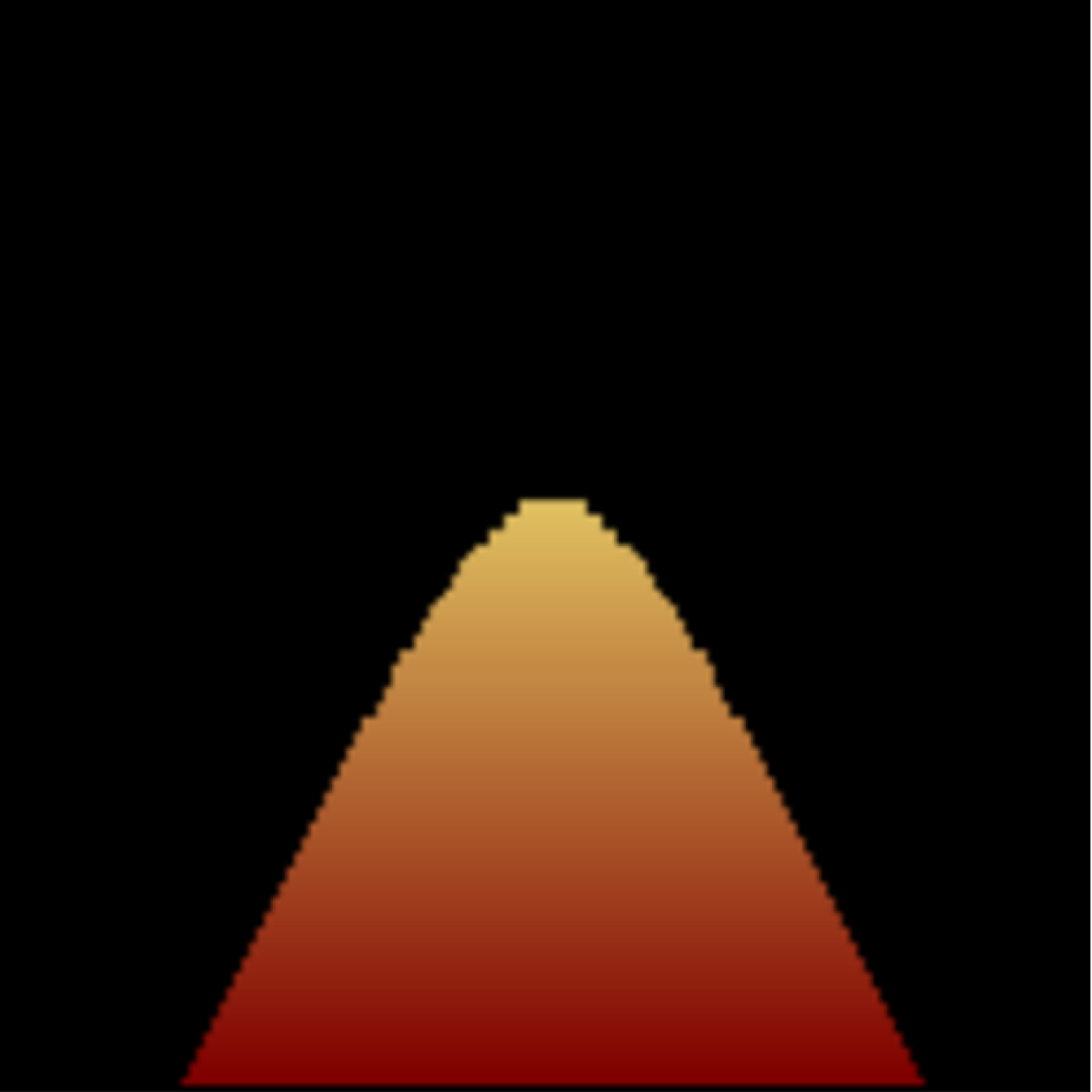
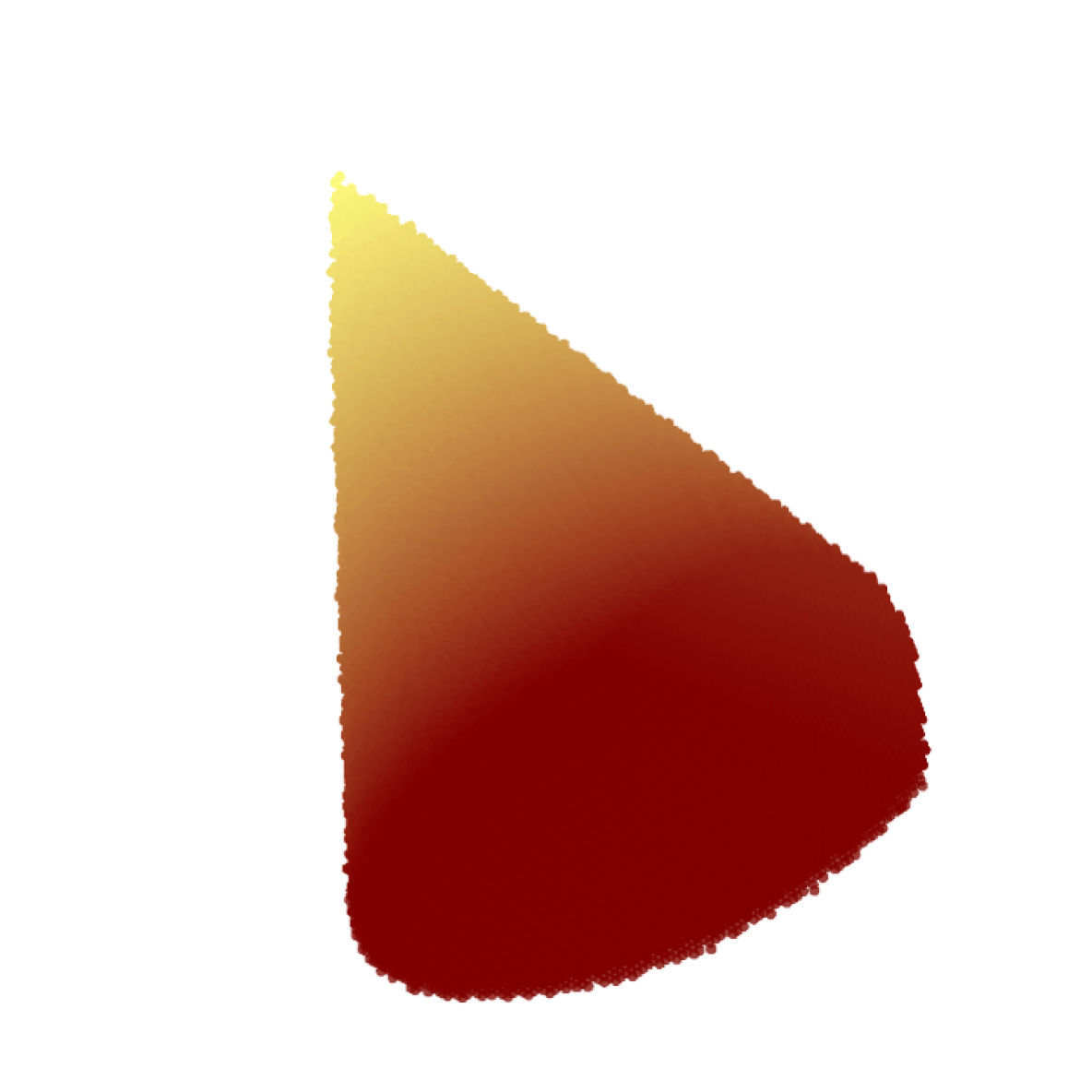
Figure XII: Synthetic Cone Generation with X-Diffusion. Top left image is the input to the model. We show (top): the generated 3D cone and slices from the 3D volume, (bottom): the ground-truth 3D cone and corresponding slices from 3D volume.

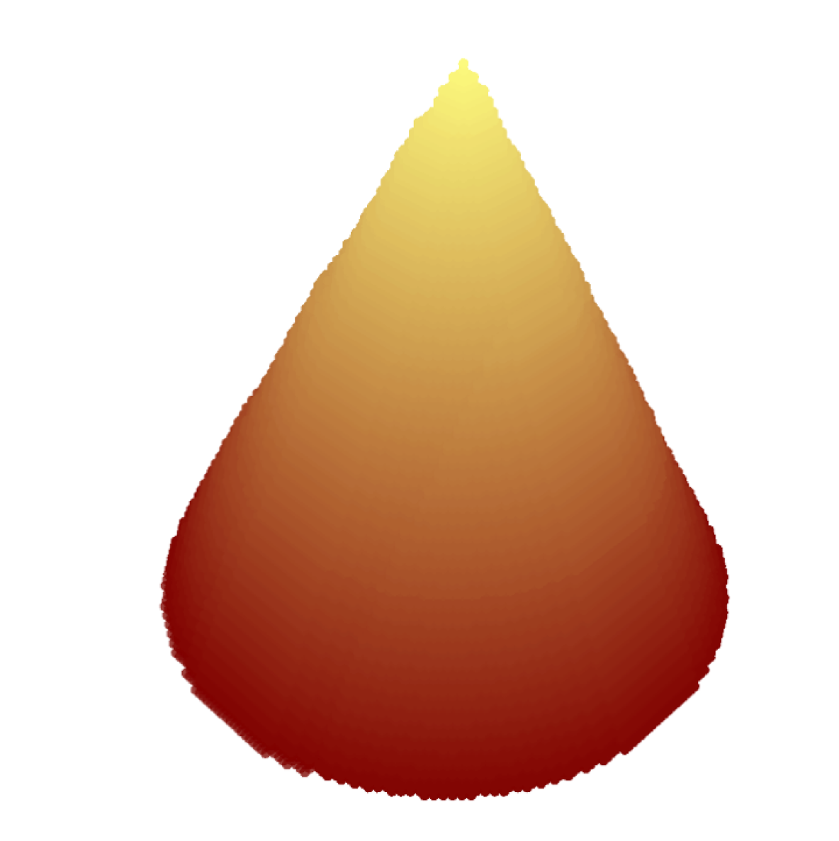
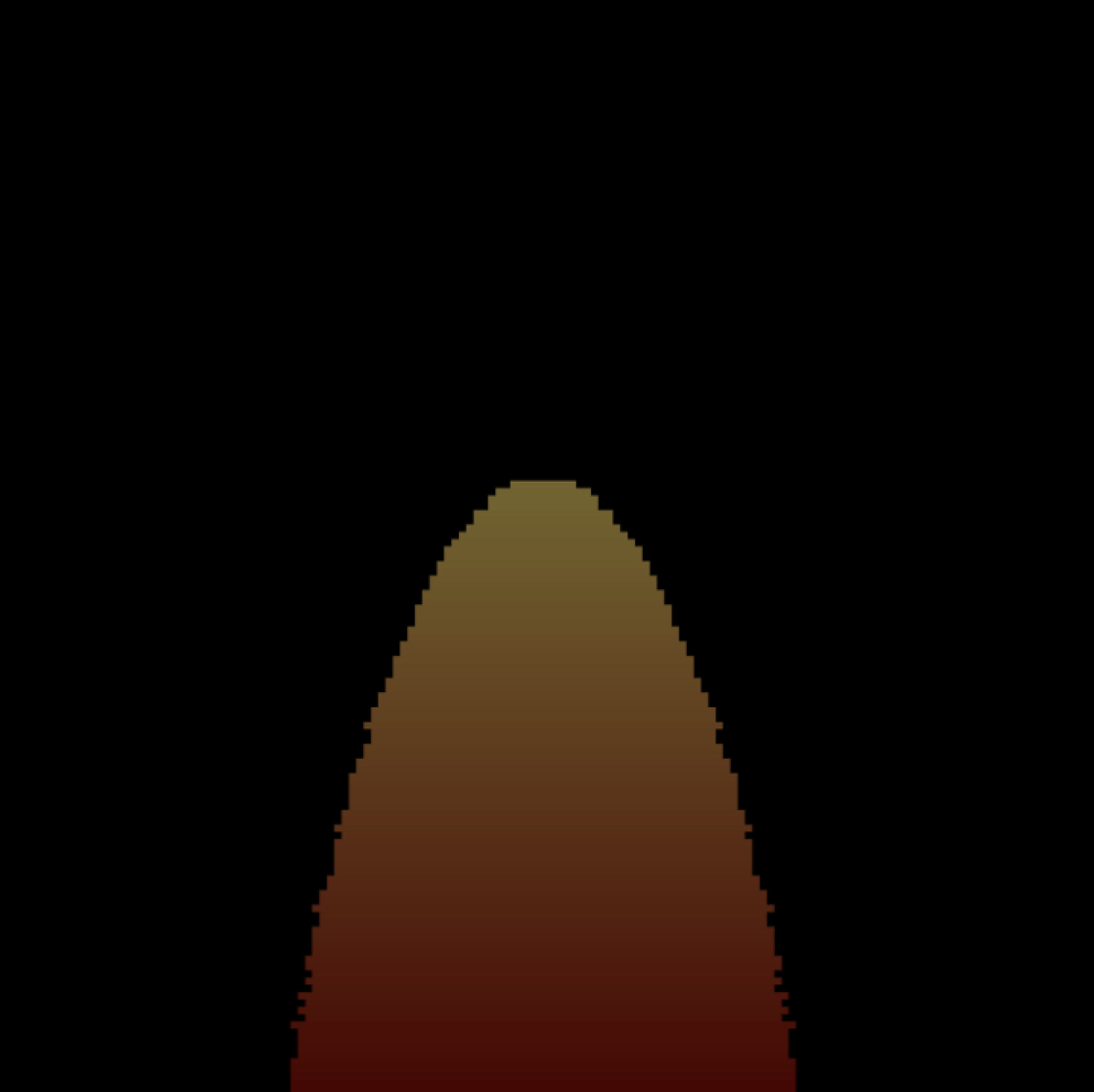
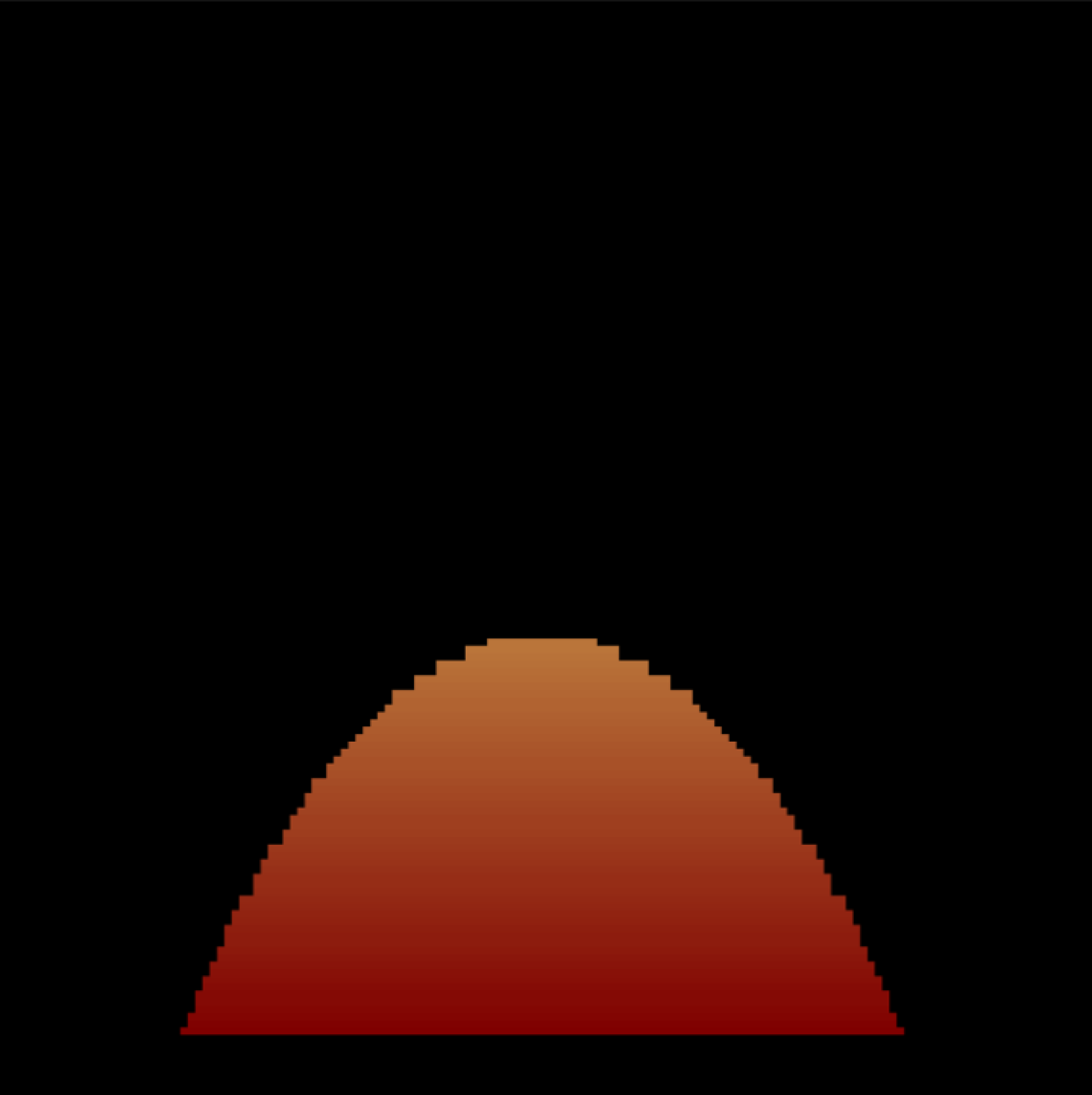
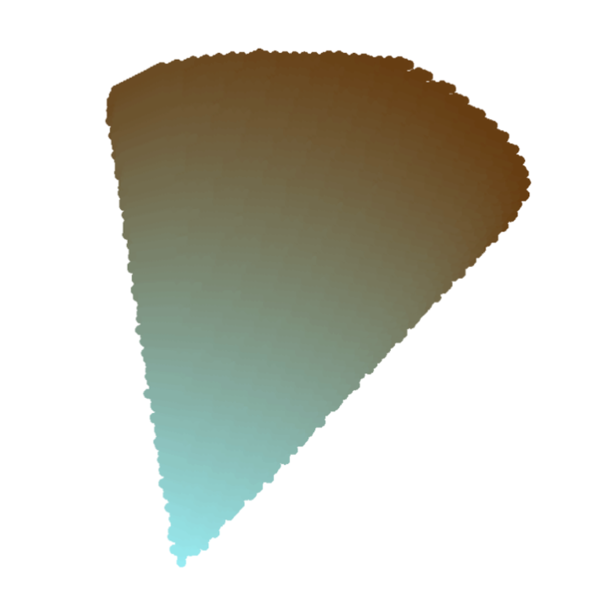
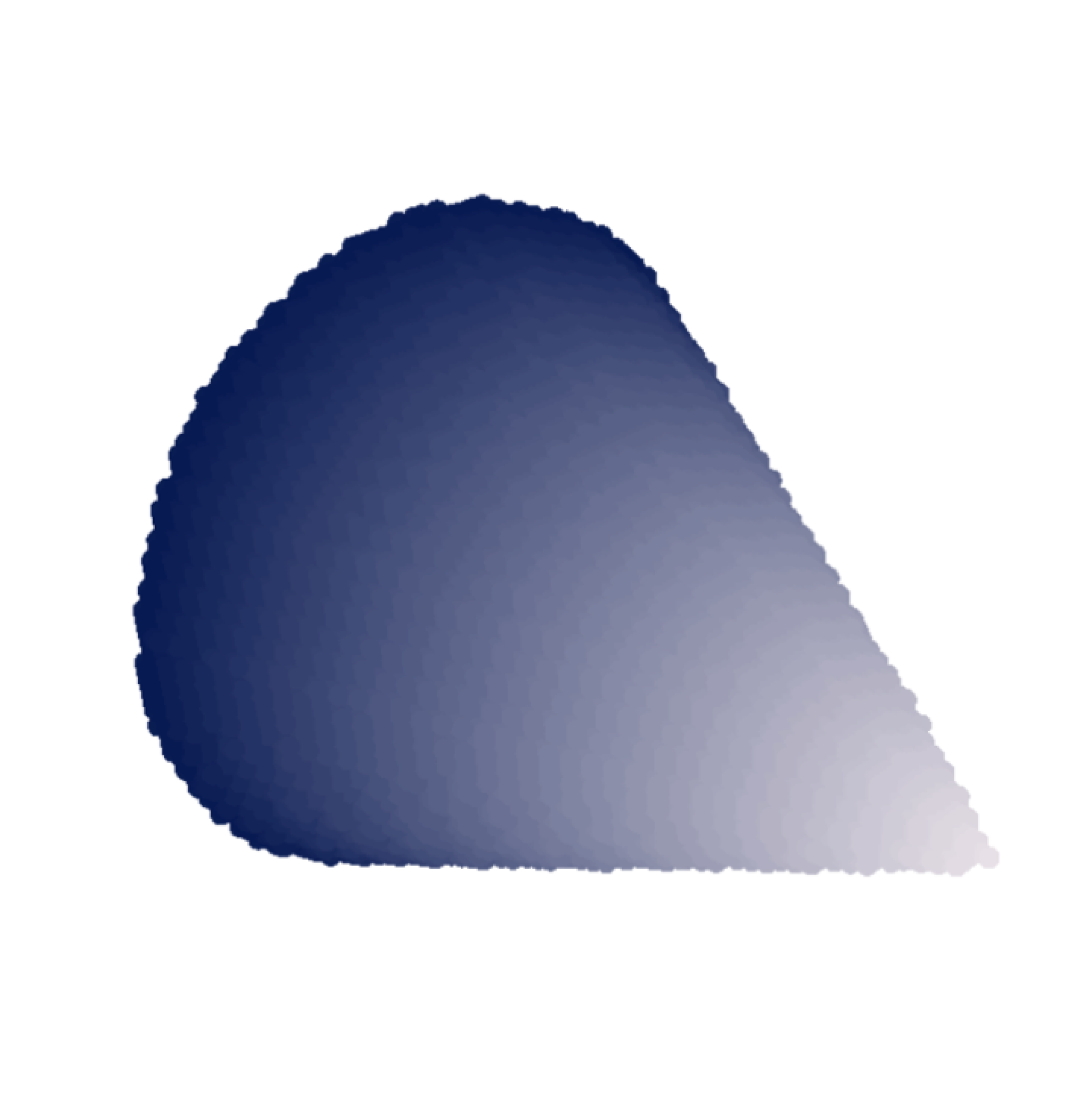
Figure XIII: Synthetic Volume Dataset. We show some samples of our proposed Synthetic Volumes dataset. The dataset consists of cones with different sizes, orientations, and colours (constant and gradient colours).

References

- [1] IXI Dataset. https://brain-development.org/ixi-dataset/, accessed: 2023-11-05
- [2] Agarwal, S., Furukawa, Y., Snavely, N., Simon, I., Curless, B., Seitz, S.M., Szeliski, R.: Building rome in a day. Communications of the ACM 54(10), 105–112 (2011)
- [3] Arnold, T.C., Freeman, C.W., Litt, B., Stein, J.M.: Low-field mri: Clinical promise and challenges. Journal of Magnetic Resonance Imaging 57(1), 25–44 (2023)
- [4] Baid, U., Ghodasara, S., Bilello, M., Mohan, S., Calabrese, E., Colak, E., Farahani, K., Kalpathy-Cramer, J., Kitamura, F.C., Pati, S., Prevedello, L.M., Rudie, J.D., Sako, C., Shinohara, R.T., Bergquist, T., Chai, R., Eddy, J.A., Elliott, J., Reade, W.C., Schaffter, T., Yu, T., Zheng, J., Annotators, B., Davatzikos, C., Mongan, J.T., Hess, C.P., Cha, S., Villanueva-Meyer, J.E., Freymann, J.B., Kirby, J.S., Wiestler, B., Crivellaro, P.S., R.Colen, R., Kotrotsou, A., Marcus, D., Milchenko, M., Nazeri, A., Fathallah-Shaykh, H.M., Wiest, R., Jakab, A., Weber, M.A., Mahajan, A., Menze, B.H., Flanders, A.E., Bakas, S.: The rsna-asnr-miccai brats 2021 benchmark on brain tumor segmentation and radiogenomic classification. ArXiv abs/2107.02314 (2021), https://api.semanticscholar.org/CorpusID:235742974
- [5] Bakas, S., Akbari, H., Sotiras, A., Bilello, M., Rozycki, M., Kirby, J., Freymann, J., Farahani, K., Davatzikos, C.: Advancing the cancer genome atlas glioma mri collections with expert segmentation labels and radiomic features. Scientific Data 4 (Sep 2017). https://doi.org/10.1038/sdata.2017.117
- [6] Barron, J.T., Mildenhall, B., Tancik, M., Hedman, P., Martin-Brualla, R., Srinivasan, P.P.: Mip-nerf: A multiscale representation for anti-aliasing neural radiance fields. In: CVPR. pp. 5855–5864 (2021)
- [7] Barron, J.T., Mildenhall, B., Verbin, D., Srinivasan, P.P., Hedman, P.: Mip-nerf 360: Unbounded anti-aliased neural radiance fields. In: CVPR. pp. 5470–5479 (2022)
- [8] Bell, R.A.: Economics of mri technology. Journal of Magnetic Resonance Imaging 6(1), 10–25 (1996)
- [9] Ben-Eliezer, N., Sodickson, D.K., Shepherd, T., Wiggins, G.C., Block, K.T.: Accelerated and motion-robust in vivo t 2 mapping from radially undersampled data using bloch-simulation-based iterative reconstruction. Magnetic resonance in medicine 75(3), 1346–1354 (2016)
- [10] Bourigault, E., Jamaludin, A., Clark, E., Fairbank, J., Kadir, T., Zisserman, A.: 3d shape analysis of scoliosis. In: MICCAI Workshop on Shape in Medical Imaging. Springer (2023)
- [11] Bourigault, E., Jamaludin, A., Kadir, T., Zisserman, A.: Scoliosis measurement on DXA scans using a combined deep learning and spinal geometry approach. In: Medical Imaging with Deep Learning (2022)
- [12] Brigham, E.O., Morrow, R.E.: The fast fourier transform. IEEE Spectrum 4(12), 63–70 (1967). https://doi.org/10.1109/MSPEC.1967.5217220
- [13] Cao, H., Wang, Y., Chen, J., Jiang, D., Zhang, X., Tian, Q., Wang, M.: Swin-unet: Unet-like pure transformer for medical image segmentation. In: European conference on computer vision. pp. 205–218. Springer (2022)
- [14] Caron, M., Touvron, H., Misra, I., Jégou, H., Mairal, J., Bojanowski, P., Joulin, A.: Emerging properties in self-supervised vision transformers. In: CVPR. pp. 9650–9660 (2021)
- [15] Chen, R., Chen, Y., Jiao, N., Jia, K.: Fantasia3d: Disentangling geometry and appearance for high-quality text-to-3d content creation. arXiv preprint arXiv:2303.13873 (2023)
- [16] Chen, Y., Ruan, D., Xiao, J., Wang, L., Sun, B., Saouaf, R., Yang, W., Li, D., Fan, Z.: Fully automated multi-organ segmentation in abdominal magnetic resonance imaging with deep neural networks. Medical physics (2019), https://api.semanticscholar.org/CorpusID:209444984
- [17] Chung, H., Ryu, D., McCann, M.T., Klasky, M.L., Ye, J.C.: Solving 3d inverse problems using pre-trained 2d diffusion models. In: Proceedings of the IEEE/CVF Conference on Computer Vision and Pattern Recognition. pp. 22542–22551 (2023)
- [18] Chung, H., Sim, B., Ryu, D., Ye, J.C.: Improving diffusion models for inverse problems using manifold constraints. Advances in Neural Information Processing Systems 35, 25683–25696 (2022)
- [19] Chung, H., Ye, J.C.: Score-based diffusion models for accelerated mri. Medical Image Analysis p. 102479 (2022)
- [20] Deitke, M., Schwenk, D., Salvador, J., Weihs, L., Michel, O., VanderBilt, E., Schmidt, L., Ehsani, K., Kembhavi, A., Farhadi, A.: Objaverse: A universe of annotated 3d objects. In: IEEE Conf. Comput. Vis. Pattern Recog. pp. 13142–13153 (2023)
- [21] Dikici, E., Ryu, J.L., Demirer, M., Bigelow, M.T., White, R.D., Slone, W.H., Erdal, B.S., Prevedello, L.M.: Automated brain metastases detection framework for t1-weighted contrast-enhanced 3d mri. IEEE Journal of Biomedical and Health Informatics 24, 2883–2893 (2019), https://api.semanticscholar.org/CorpusID:199551987
- [22] Doran, S.J., Hipwell, J.H., Denholm, R., Eiben, B., Marta, Busana, Hawkes, D.J., Leach, M.O., dos Santos Silva, I.: Breast mri segmentation for density estimation breast mri segmentation for density estimation: Do different methods (2017), https://api.semanticscholar.org/CorpusID:55077584
- [23] Faugeras, O.D.: What can be seen in three dimensions with an uncalibrated stereo rig? In: Computer Vision—ECCV’92: Second European Conference on Computer Vision Santa Margherita Ligure, Italy, May 19–22, 1992 Proceedings 2. pp. 563–578. Springer (1992)
- [24] Fessler, J.A.: Model-based image reconstruction for mri. IEEE Signal Processing Magazine 27(4), 81–89 (2010). https://doi.org/10.1109/MSP.2010.936726
- [25] Hamdi, A., Ghanem, B., Nießner, M.: Sparf: Large-scale learning of 3d sparse radiance fields from few input images. arxiv (2022)
- [26] Hamdi, A., Giancola, S., Ghanem, B.: Mvtn: Multi-view transformation network for 3d shape recognition. In: Proceedings of the IEEE/CVF International Conference on Computer Vision (ICCV). pp. 1–11 (October 2021)
- [27] Hamdi, A., Giancola, S., Ghanem, B.: Voint cloud: Multi-view point cloud representation for 3d understanding. In: The Eleventh International Conference on Learning Representations (2023), https://openreview.net/forum?id=IpGgfpMucHj
- [28] Hatamizadeh, A., Nath, V., Tang, Y., Yang, D., Roth, H.R., Xu, D.: Swin unetr: Swin transformers for semantic segmentation of brain tumors in mri images. ArXiv abs/2201.01266 (2022), https://api.semanticscholar.org/CorpusID:245668780
- [29] Hong, F., Zhang, M., Pan, L., Cai, Z., Yang, L., Liu, Z.: Avatarclip: Zero-shot text-driven generation and animation of 3d avatars. arXiv preprint arXiv:2205.08535 (2022)
- [30] Jain, A., Mildenhall, B., Barron, J.T., Abbeel, P., Poole, B.: Zero-shot text-guided object generation with dream fields. In: IEEE Conf. Comput. Vis. Pattern Recog. pp. 867–876 (2022)
- [31] Jain, A., Tancik, M., Abbeel, P.: Putting nerf on a diet: Semantically consistent few-shot view synthesis. In: CVPR. pp. 5885–5894 (2021)
- [32] Jamaludin, A., Fairbank, J., Harding, I., Kadir, T., Peters, T.J., Zisserman, A., Clark, E.M.: Identifying scoliosis in population-based cohorts: Automation of a validated method based on total body dual energy x-ray absorptiometry scans (2020)
- [33] Jamaludin, A., Kadir, T., Zisserman, A.: Self-supervised learning for spinal mris. ArXiv abs/1708.00367 (2017), https://api.semanticscholar.org/CorpusID:9549581
- [34] Jiang, M., Zhi, M., Wei, L., Yang, X., Zhang, J., Li, Y., Wang, P., Huang, J., Yang, G.: Fa-gan: Fused attentive generative adversarial networks for mri image super-resolution (2021)
- [35] Kawar, B., Elad, M., Ermon, S., Song, J.: Denoising diffusion restoration models. In: Advances in Neural Information Processing Systems (2022)
- [36] Kim, M., Seo, S., Han, B.: Infonerf: Ray entropy minimization for few-shot neural volume rendering. In: CVPR. pp. 12912–12921 (2022)
- [37] Knoll, F., Zbontar, J., Sriram, A., Muckley, M., Bruno, M., Defazio, A., Parente, M., Geras, K.J., Katsnelson, J., Chandarana, H., Zhang, Z., Drozdzalv, M., Romero, A., Rabbat, M.G., Vincent, P., Pinkerton, J., Wang, D., Yakubova, N., Owens, E., Zitnick, C.L., Recht, M.P., Sodickson, D.K., Lui, Y.W.: fastmri: A publicly available raw k-space and dicom dataset of knee images for accelerated mr image reconstruction using machine learning. Radiology. Artificial intelligence 2 1, e190007 (2020), https://api.semanticscholar.org/CorpusID:211214833
- [38] Langner, T., Mora, A., Strand, R., Ahlström, H., Kullberg, J.: Mimir: Deep regression for automated analysis of uk biobank body mri. ArXiv abs/2106.11731 (2021), https://api.semanticscholar.org/CorpusID:235593053
- [39] Lee, S., Chung, H., Park, M., Park, J., Ryu, W.S., Ye, J.C.: Improving 3d imaging with pre-trained perpendicular 2d diffusion models. In: Proceedings of the IEEE/CVF International Conference on Computer Vision (ICCV). pp. 10710–10720 (October 2023)
- [40] Lin, C.H., Gao, J., Tang, L., Takikawa, T., Zeng, X., Huang, X., Kreis, K., Fidler, S., Liu, M.Y., Lin, T.Y.: Magic3d: High-resolution text-to-3d content creation. In: CVPR (2023)
- [41] Liu, R., Wu, R., Van Hoorick, B., Tokmakov, P., Zakharov, S., Vondrick, C.: Zero-1-to-3: Zero-shot one image to 3d object. arXiv preprint arXiv:2303.11328 (2023)
- [42] Lombardi, S., Simon, T., Saragih, J., Schwartz, G., Lehrmann, A., Sheikh, Y.: Neural volumes: Learning dynamic renderable volumes from images. ACM Trans. Graph. 38(4), 65:1–65:14 (Jul 2019). https://doi.org/10.1145/3306346.3323020, http://doi.acm.org/10.1145/3306346.3323020
- [43] Ma, J., Wang, B.: Segment anything in medical images. arXiv preprint arXiv:2304.12306 (2023)
- [44] Melas-Kyriazi, L., Rupprecht, C., Laina, I., Vedaldi, A.: Realfusion: 360deg reconstruction of any object from a single image. In: CVPR (2023)
- [45] Menze, B., Jakab, A., Bauer, S., Kalpathy-Cramer, J., Farahani, K., Kirby, J., Burren, Y., Porz, N., Slotboom, J., Wiest, R., Van Leemput, K.: The multimodal brain tumor image segmentation benchmark (brats). I E E E Transactions on Medical Imaging 34(10), 1993 – 2024 (2015). https://doi.org/10.1109/TMI.2014.2377694
- [46] Menze, B.H., Jakab, A., Bauer, S., Kalpathy-Cramer, J., Farahani, K., Kirby, J.S., Burren, Y., Porz, N., Slotboom, J., Wiest, R., Lanczi, L., Gerstner, E.R., Weber, M.A., Arbel, T., Avants, B.B., Ayache, N., Buendia, P., Collins, D.L., Cordier, N., Corso, J.J., Criminisi, A., Das, T., Delingette, H., Çağatay Demiralp, Durst, C.R., Dojat, M., Doyle, S., Festa, J., Forbes, F., Geremia, E., Glocker, B., Golland, P., Guo, X., Hamamci, A., Iftekharuddin, K.M., Jena, R., John, N.M., Konukoglu, E., Lashkari, D., Mariz, J.A., Meier, R., Pereira, S., Precup, D., Price, S.J., Riklin-Raviv, T., Reza, S.M.S., Ryan, M.T., Sarikaya, D., Schwartz, L.H., Shin, H.C., Shotton, J., Silva, C.A., Sousa, N.J., Subbanna, N.K., Székely, G., Taylor, T.J., Thomas, O.M., Tustison, N., Ünal, G.B., Vasseur, F., Wintermark, M., Ye, D.H., Zhao, L., Zhao, B., Zikic, D., Prastawa, M., Reyes, M., Leemput, K.V.: The multimodal brain tumor image segmentation benchmark (brats). IEEE Transactions on Medical Imaging 34, 1993–2024 (2015), https://api.semanticscholar.org/CorpusID:1739295
- [47] Mildenhall, B., Srinivasan, P.P., Tancik, M., Barron, J.T., Ramamoorthi, R., Ng, R.: Nerf: Representing scenes as neural radiance fields for view synthesis. In: European conference on computer vision. pp. 405–421. Springer (2020)
- [48] Mohammad Khalid, N., Xie, T., Belilovsky, E., Popa, T.: Clip-mesh: Generating textured meshes from text using pretrained image-text models. In: SIGGRAPH Asia 2022 Conference Papers. pp. 1–8 (2022)
- [49] Nguyen, D.M., Nguyen, H., Diep, N.T., Pham, T.N., Cao, T., Nguyen, B.T., Swoboda, P., Ho, N., Albarqouni, S., Xie, P., et al.: Lvm-med: Learning large-scale self-supervised vision models for medical imaging via second-order graph matching. arXiv preprint arXiv:2306.11925 (2023)
- [50] OpenAI: Gpt-4 technical report (2023)
- [51] Poole, B., Jain, A., Barron, J.T., Mildenhall, B.: Dreamfusion: Text-to-3d using 2d diffusion. ICLR (2022)
- [52] Qian, G., Mai, J., Hamdi, A., Ren, J., Siarohin, A., Li, B., Lee, H.Y., Skorokhodov, I., Wonka, P., Tulyakov, S., et al.: Magic123: One image to high-quality 3d object generation using both 2d and 3d diffusion priors. arXiv preprint arXiv:2306.17843 (2023)
- [53] Quan, T.M., Nguyen-Duc, T., Jeong, W.K.: Compressed sensing mri reconstruction using a generative adversarial network with a cyclic loss. IEEE Transactions on Medical Imaging 37, 1488–1497 (2017), https://api.semanticscholar.org/CorpusID:3898199
- [54] Radford, A., Kim, J.W., Hallacy, C., Ramesh, A., Goh, G., Agarwal, S., Sastry, G., Askell, A., Mishkin, P., Clark, J., et al.: Learning transferable visual models from natural language supervision. In: ICML. pp. 8748–8763. PMLR (2021)
- [55] Ranjbarzadeh, R., Kasgari, A.B., Ghoushchi, S.J., Anari, S., Naseri, M., Bendechache, M.: Brain tumor segmentation based on deep learning and an attention mechanism using mri multi-modalities brain images. Scientific Reports 11 (2021), https://api.semanticscholar.org/CorpusID:235198255
- [56] Roeloffs, V., Wang, X., Sumpf, T.J., Untenberger, M., Voit, D., Frahm, J.: Model-based reconstruction for t1 mapping using single-shot inversion-recovery radial flash. International Journal of Imaging Systems and Technology 26(4), 254–263 (2016)
- [57] Rombach, R., Blattmann, A., Lorenz, D., Esser, P., Ommer, B.: High-resolution image synthesis with latent diffusion models. In: CVPR. pp. 10684–10695 (2022)
- [58] Ronneberger, O., Fischer, P., Brox, T.: U-net: Convolutional networks for biomedical image segmentation. In: Navab, N., Hornegger, J., Wells, W.M., Frangi, A.F. (eds.) Medical Image Computing and Computer-Assisted Intervention – MICCAI 2015. pp. 234–241. Springer International Publishing, Cham (2015)
- [59] Saharia, C., Chan, W., Saxena, S., Li, L., Whang, J., Denton, E.L., Ghasemipour, K., Gontijo Lopes, R., Karagol Ayan, B., Salimans, T., et al.: Photorealistic text-to-image diffusion models with deep language understanding. NeurIPS 35, 36479–36494 (2022)
- [60] Sarracanie, M., LaPierre, C.D., Salameh, N., Waddington, D.E., Witzel, T., Rosen, M.S.: Low-cost high-performance mri. Scientific reports 5(1), 15177 (2015)
- [61] Schlemper, J., Caballero, J., Hajnal, J.V., Price, A.N., Rueckert, D.: A deep cascade of convolutional neural networks for dynamic mr image reconstruction. IEEE Transactions on Medical Imaging 37, 491–503 (2017), https://api.semanticscholar.org/CorpusID:18068061
- [62] Seo, H., Kim, H., Kim, G., Chun, S.Y.: Ditto-nerf: Diffusion-based iterative text to omni-directional 3d model. arXiv preprint arXiv:2304.02827 (2023)
- [63] Sohl-Dickstein, J., Weiss, E., Maheswaranathan, N., Ganguli, S.: Deep unsupervised learning using nonequilibrium thermodynamics. In: ICML. pp. 2256–2265. PMLR (2015)
- [64] Song, Y., Sohl-Dickstein, J., Kingma, D.P., Kumar, A., Ermon, S., Poole, B.: Score-based generative modeling through stochastic differential equations. In: International Conference on Learning Representations (2021), https://openreview.net/forum?id=PxTIG12RRHS
- [65] Song, Y., Sohl-Dickstein, J.N., Kingma, D.P., Kumar, A., Ermon, S., Poole, B.: Score-based generative modeling through stochastic differential equations. ArXiv abs/2011.13456 (2020), https://api.semanticscholar.org/CorpusID:227209335
- [66] Su, H., Maji, S., Kalogerakis, E., Learned-Miller, E.: Multi-view convolutional neural networks for 3d shape recognition. In: Proceedings of the IEEE international conference on computer vision. pp. 945–953 (2015)
- [67] Sudlow, C.L.M., Gallacher, J.E., Allen, N.E., Beral, V., Burton, P., Danesh, J., Downey, P., Elliott, P., Green, J., Landray, M.J., Liu, B.C., Matthews, P.M., Ong, G., Pell, J.P., Silman, A.J., Young, A., Sprosen, T., Peakman, T.C., Collins, R.: Uk biobank: An open access resource for identifying the causes of a wide range of complex diseases of middle and old age. PLoS Medicine 12 (2015)
- [68] Tan, Z., Roeloffs, V., Voit, D., Joseph, A.A., Untenberger, M., Merboldt, K.D., Frahm, J.: Model-based reconstruction for real-time phase-contrast flow mri: improved spatiotemporal accuracy. Magnetic resonance in medicine 77(3), 1082–1093 (2017)
- [69] Tang, J., Wang, T., Zhang, B., Zhang, T., Yi, R., Ma, L., Chen, D.: Make-it-3d: High-fidelity 3d creation from a single image with diffusion prior. arXiv preprint arXiv:2303.14184 (2023)
- [70] Tang, Y., Yang, D., Li, W., Roth, H.R., Landman, B.A., Xu, D., Nath, V., Hatamizadeh, A.: Self-supervised pre-training of swin transformers for 3d medical image analysis. 2022 IEEE/CVF Conference on Computer Vision and Pattern Recognition (CVPR) pp. 20698–20708 (2021), https://api.semanticscholar.org/CorpusID:244715046
- [71] Tran, D., Bourdev, L., Fergus, R., Torresani, L., Paluri, M.: Learning spatiotemporal features with 3d convolutional networks. In: Proceedings of the IEEE International Conference on Computer Vision (ICCV). pp. 4489–4497 (2015)
- [72] Tran-Gia, J., Stäb, D., Wech, T., Hahn, D., Köstler, H.: Model-based acceleration of parameter mapping (map) for saturation prepared radially acquired data. Magnetic resonance in medicine 70(6), 1524–1534 (2013)
- [73] Verbin, D., Hedman, P., Mildenhall, B., Zickler, T., Barron, J.T., Srinivasan, P.P.: Ref-nerf: Structured view-dependent appearance for neural radiance fields. In: CVPR. pp. 5481–5490. IEEE (2022)
- [74] Wald, L.L., McDaniel, P.C., Witzel, T., Stockmann, J.P., Cooley, C.Z.: Low-cost and portable mri. Journal of Magnetic Resonance Imaging 52(3), 686–696 (2020)
- [75] Wang, X., Roeloffs, V., Klosowski, J., Tan, Z., Voit, D., Uecker, M., Frahm, J.: Model-based t 1 mapping with sparsity constraints using single-shot inversion-recovery radial flash. Magnetic resonance in medicine 79(2), 730–740 (2018)
- [76] Wang, Z., Bovik, A.C., Sheikh, H.R., Simoncelli, E.P.: Image quality assessment: From error visibility to structural similarity. IEEE TRANSACTIONS ON IMAGE PROCESSING 13, NO. 4 (2004)
- [77] Windsor, R., Jamaludin, A.: The ladder algorithm: Finding repetitive structures in medical images by induction. 2020 IEEE 17th International Symposium on Biomedical Imaging (ISBI) pp. 1729–1733 (2020), https://api.semanticscholar.org/CorpusID:210965990
- [78] Windsor, R., Jamaludin, A., Kadir, T., Zisserman, A.: A convolutional approach to vertebrae detection and labelling in whole spine mri. In: International Conference on Medical Image Computing and Computer-Assisted Intervention (2020), https://api.semanticscholar.org/CorpusID:220364469
- [79] Windsor, R., Jamaludin, A., Kadir, T., Zisserman, A.: Self-supervised multi-modal alignment for whole body medical imaging. In: International Conference on Medical Image Computing and Computer Assisted Intervention (2021)
- [80] Xu, J., Wang, X., Cheng, W., Cao, Y.P., Shan, Y., Qie, X., Gao, S.: Dream3d: Zero-shot text-to-3d synthesis using 3d shape prior and text-to-image diffusion models. In: Proceedings of the IEEE/CVF Conference on Computer Vision and Pattern Recognition (CVPR). pp. 20908–20918 (June 2023)
- [81] Yu, A., Ye, V., Tancik, M., Kanazawa, A.: pixelnerf: Neural radiance fields from one or few images. In: CVPR. pp. 4578–4587 (2021)
- [82] Zbontar, J., Knoll, F., Sriram, A., Murrell, T., Huang, Z., Muckley, M.J., Defazio, A., Stern, R., Johnson, P., Bruno, M., Parente, M., Geras, K.J., Katsnelson, J., Chandarana, H., Zhang, Z., Drozdzal, M., Romero, A., Rabbat, M., Vincent, P., Yakubova, N., Pinkerton, J., Wang, D., Owens, E., Zitnick, C.L., Recht, M.P., Sodickson, D.K., Lui, Y.W.: fastmri: An open dataset and benchmarks for accelerated mri (2019)
- [83] Zhou, Z., Siddiquee, M.M.R., Tajbakhsh, N., Liang, J.: Unet++: A nested u-net architecture for medical image segmentation. Deep Learning in Medical Image Analysis and Multimodal Learning for Clinical Decision Support : 4th International Workshop, DLMIA 2018, and 8th International Workshop, ML-CDS 2018, held in conjunction with MICCAI 2018, Granada, Spain, S… 11045, 3–11 (2018), https://api.semanticscholar.org/CorpusID:50786304