Nonlinear scalarization of Schwarzschild black holes in Einstein-scalar-Gauss-Bonnet gravity

Abstract

In this paper, we propose a fully nonlinear mechanism for obtaining scalarized black holes in Einstein-scalar-Gauss-Bonnet (EsGB) gravity which is beyond the spontaneous scalarization. Introducing three coupling functions $f(\varphi)$ satisfying $f^{\prime\prime}(0)=0$, we find that Schwarzschild black hole is linearly stable against scalar perturbation, whereas it is unstable against nonlinear scalar perturbation if the coupling function includes term higher than $\varphi^{6}$. For a specific choice of coupling function $f(\varphi)=\alpha(\varphi^{4}-\beta\varphi^{6})$, we obtain new black holes with scalar hair in the EsGB gravity. In this case, the coupling parameter $\alpha$ plays a major role in making different nonlinear scalarized black holes, while the other parameter $\beta$ plays a supplementary role. Furthermore, we study thermodynamic aspects of these scalarized black holes and prove the first-law of thermodynamics.

I Introduction

It is worth noting that scalar fields ubiquitously appear in the various contexts of theoretical physics, and offer a straightforward and versatile framework that accounts for the accelerated expansion of the universe, both in its early stages and in its later epochs. In addition, physics of black holes can probe the existence of scalar fields from the completely different aspects. In general relativity (GR), however, the no-hair theorem rules out black holes conformally coupled to a scalar field in asymptotically flat spacetimes due to a divergent scalar on the horizon and instability of black holes Bekenstein:1974sf -Bekenstein:1995un . Then, it becomes a challenge to introduce scalar fields that interact with the curvature of black hole spacetimes. Fortunately, the no-theorem can be circumvented when hairy black holes possess extra macroscopic degrees of freedom in other theories. For instance, Damour and Esposito-Farese Damour:1993hw have shown a mechanism of spontaneous scalarization in scalar-tensor gravity when studying neutron stars.

As one of scalar-tensor gravity theories, Einstein-scalar-Gauss-Bonnet (EsGB) gravity has received increasing attentions over the past years. The merits of this theory lie in twofold. Firstly, it makes a simple modification of GR by including the Gauss-Bonnet curvature term coupled to a single scalar field. Secondly, since this term alone is a topological term in four dimensional spacetimes, this theory corresponds to extending GR rather than modifying it, provided that all solutions of GR are also solutions of these theories and they can coexist with non-GR solutions. The Refs. Doneva:2017bvd -Antoniou:2017acq have shown that the spontaneous scalarization may take place around Schwarzschild black holes in EsGB gravity, due to a tachyonic instability triggered by coupling a scalar field to the Gauss-Bonnet term [$f(\varphi){\mathcal{R}^{2}}_{\rm GB}$]. This is analogous to relativistic stars triggered by coupling a scalar field to the matter field. Then, a new branch of black hole solutions with nontrivial scalar field bifurcates from the Schwarzschild solution. Similar discussions have been also presented in the context of scalar-tensor gravity theories possessing the scalar field non-minimally coupled to either Gauss-Bonnet term Antoniou:2017hxj -Berti:2020kgk or to Maxwell term [$f(\varphi)F^{2}$] Herdeiro:2018wub -Promsiri:2023yda , where the scalar field induces destabilization of bald black holes and makes scalarized (charged) black holes. It is important to note that infinite branches ($n=0,~{}1,~{}2,~{}\cdots$) of scalarized (charged) black holes are generated through spontaneous scalarization.

Concerning nonlinear scalarization of Schwarzschild black holes in the EsGB gravity, the effective mass term of a perturbed scalar always vanishes when the coupling function takes the following exponential forms:

$$f(\varphi)=\frac{1}{4\kappa}\left(1-e^{-\kappa\varphi^{4}}\right)\quad{\rm or}\quad\frac{1}{4\kappa}\left(1-e^{-\kappa\varphi^{6}}\right).$$ (1)

It implies that Schwarzschild black holes are always stable under a linear scalar perturbation. Nevertheless, it is interesting to note that Schwarzschild black holes become unstable against nonlinear scalar perturbation when the amplitude of a scalar perturbation is large enough Doneva:2021tvn -Zhang:2023jei . Here, finite (three) branches of scalarized black holes for $\kappa=100$ appear but only one branch is stable against radial perturbations Blazquez-Salcedo:2022omw . Evolving nonlinear scalar equation in time on the Kerr background, Doneva et al. Doneva:2022yqu have found the nonlinear scalarization phenomenon for exponential coupling functions in the EsGB gravity. In this case, there is a threshold amplitude of the scalar perturbation above which the Kerr black hole loses the linear stability, and scalarized rotating black holes are obtained. Later, Lai, et al. Lai:2023gwe have constructed finite (three) branches of nonlinear scalarized rotating black hole solutions for the first coupling function in Eq.(1) with $\kappa=400$ by making use of the pseudo-spectral method. Thermodynamic aspect of these branches is compared to that of Kerr black hole.

In this paper, we focus on exploring the nonlinear scalarization phenomenon and examine the nonlinear instability of Schwarzschild black holes against nonlinear scalar perturbation in the EsGB gravity by choosing three polynomial coupling functions $f(\varphi)$ satisfying $f^{\prime\prime}(0)=0$, appearing in Eq.(10). The Schwarzschild black hole is unstable against nonlinear scalar perturbation if the coupling function includes term higher than $\varphi^{6}$. For a particular coupling function of $f(\varphi)=\alpha(\varphi^{4}-\beta\varphi^{6})$, we will find newly black holes with scalar hair in the EsGB gravity. In this case, the coupling parameter $\alpha$ plays a major role in making different nonlinear scalarized black holes, while the other parameter $\beta$ may play a supplementary role. Furthermore, we wish to study thermodynamic aspects of these nonlinear scalarized black holes.

The manuscript is organized as follows. We first introduce the EsGB gravity theory and discuss what is the nonlinear instability of Schwarzschild black holes by solving the scalar equation numerically in Section II. Then, we obtain numerical scalarized black hole solutions and analyze thermodynamic properties of these scalarzied black holes in Section III. Finally, Section IV is ready for conclusions and discussions.

II Nonlinear instability of Schwarzschild black holes

We start with the Einstein-scalar-Gauss-Bonnet (EsGB) gravity theory, whose action is given by Doneva:2017bvd

$$\mathcal{S}=\frac{1}{{16\pi}}\int{{d^{4}}}x\sqrt{-g}\left[{R-2{\nabla_{\mu}}\varphi{\nabla^{\mu}}\varphi+{\lambda^{2}}f(\varphi){\mathcal{R}^{2}}_{\rm GB}}\right],\$$ (2)

where $R$ is the Ricci scalar and ${R^{2}}_{\rm GB}={R_{\mu\nu\rho\sigma}}{R^{\mu\nu\rho\sigma}}-4{R_{\mu\nu}}{R^{\mu\nu}}+{R^{2}}$ is so-called Gauss-Bonnet curvature term. Moreover, $\varphi$ denotes a scalar field, $f(\varphi)$ represents a coupling function depending on $\varphi$, and $\lambda$ is the Gauss-Bonnet coupling parameter. Then, two equations can be obtained as

$${R_{\mu\nu}}-\frac{1}{2}R{g_{\mu\nu}}+{\Gamma_{\mu\nu}}=2{\nabla_{\mu}}\varphi{\nabla_{\nu}}\varphi-{g_{\mu\nu}}{\nabla_{\alpha}}\varphi{\nabla^{a}}\varphi,$$ (3)

$$\square\varphi=-\frac{\lambda^{2}}{4}\frac{{df(\varphi)}}{{d\varphi}}{\mathcal{R}^{2}}_{GB},$$ (4)

where $\Gamma_{\mu\nu}$ is defined by

$${\Gamma_{\mu\nu}} = -R({\nabla_{\mu}}{\psi_{\nu}}+{\nabla_{\nu}}{\psi_{\mu}})-4{\nabla^{\alpha}}{\psi_{\alpha}}\left({{R_{\mu\nu}}-\frac{1}{2}R{g_{\mu\nu}}}\right)+4{R_{\mu\alpha}}{\nabla^{\alpha}}{\psi_{\nu}}$$ (5)

$$+4{R_{\nu\alpha}}{\nabla^{\alpha}}{\psi_{\mu}}-4{g_{\mu\nu}}{R^{\alpha\beta}}{\nabla_{\alpha}}{\psi_{\beta}}+4{R^{\beta}}_{\mu\alpha\nu}\nabla_{\alpha}{\psi_{\beta}}$$

with

$${\psi_{\mu}}={\lambda^{2}}\frac{{df(\varphi)}}{{d\varphi}}{\nabla_{\mu}}\varphi.$$

In the EsGB gravity, the linearized Einstein equation ($\delta G_{\mu\nu}(h)=0$) governing the metric perturbation $\delta g_{\mu\nu}=h_{\mu\nu}$ are decoupled from the scalar equation governing the scalar perturbation $\delta\phi$. Then, this linearized Einstein equation is the same as that for the Einstein gravity and, it turns out that Schwarzschild black hole is stable against the metric perturbation $h_{\mu\nu}$. Therefore, we shall focus only on the linearized scalar equation

$$\bar{\square}\delta\varphi-\mu_{{\rm{eff}}}^{2}\delta\varphi=0,$$ (6)

where the effective scalar mass is given by

$$\mu_{{\rm{eff}}}^{2}=-\frac{{{\lambda^{2}}}}{4}\frac{{{d^{2}}f}}{{d{\varphi^{2}}}}(0)\bar{R}_{\rm GB}^{2}.$$ (7)

Then, spontaneous scalarization may take place around Schwarzschild black holes. The tachyonic instability is triggered by an effective scalar mass $\mu_{{\rm{eff}}}$ when the coupling function $f(\varphi)$ satisfies the following three conditions Doneva:2017bvd -Antoniou:2017acq :

$$f(0)=0,\quad\frac{{df}}{{d\varphi}}(0)=0,\quad\frac{{{d^{2}}f}}{{d{\varphi^{2}}}}(0)\neq 0.$$ (8)

Here, infinite branches ($n=0,~{}1,~{}2,~{}\cdots$) of scalarized black holes emerges from solving static linearized scalar equation [$\bar{\nabla}^{2}\delta\varphi(\bf{x})-\mu_{{\rm{eff}}}^{2}\delta\varphi(\bf{x})$].

On the other hand, if the coupling functions are given by Eq.(1), we have

$$\quad\frac{{{d^{2}}f}}{{d{\varphi^{2}}}}(0)=0\to\mu_{{\rm{eff}}}^{2}=0.$$ (9)

It is clear that tachyonic instability is absent because of $\bar{\square}\delta\varphi=0$ and the Schwarzschild black hole is stable against linear scalar perturbation. Nevertheless, Schwarzschild black holes allows to be unstable against nonlinear scalar perturbation when the amplitude of a scalar perturbation is large enough Doneva:2021tvn -Zhang:2023jei . This provides another mechanism to obtain scalarized black hole via nonlinear scalarization.

To realize nonlinear instability definitely, we introduce three polynomial forms of coupling functions satisfying $\frac{{{d^{2}}f}}{{d{\varphi^{2}}}}(0)=0$ as

$$f(\varphi)=\varphi^{4},\quad\varphi^{4}-\varphi^{6},\quad\varphi^{4}-\varphi^{8}.$$ (10)

Now, we introduce a mechanism to solve ($2+1$)-dimensional evolution of the Klein-Gordon Eq.(4) on the Schwarzschild background

$$ds^{2}_{\rm S}=\bar{g}_{\mu\nu}dx^{\mu}dx^{\nu}=-A(r)dt^{2}+A(r)^{-1}dr^{2}+r^{2}d\Omega^{2}\quad\text{with}\quad A(r)=1-\frac{2M}{r}.$$ (11)

After redefining the scalar field $\varphi=\frac{\Psi(t,r)}{r}$ and bringing the GB term in the background metric as

$$\mathcal{R}^{2}_{\rm GB}(\bar{g})=\frac{1}{r}\left[A(r)^{2}A^{\prime\prime}(r)-A(r)A^{\prime\prime}(r)+A(r)A^{\prime}(r)^{2}\right]\to\frac{48M^{2}}{r^{6}},$$ (12)

the Klein-Gorden equation can be simplified as

$$\begin{split}&\left(-\partial^{2}_{t}+\partial^{2}_{r_{*}}-\frac{A(r)A^{\prime}(r)}{r}\right)\Psi(t,r)\\ &+\frac{\lambda^{2}}{r}f^{\prime}(\frac{\Psi}{r})\left[A(r)^{2}A^{\prime\prime}(r)-A(r)A^{\prime\prime}(r)+A(r)A^{\prime}(r)^{2}\right]=0\end{split}$$ (13)

with the tortoise coordinate $r_{*}=\int A^{-1}(r)dr=r+2M\ln|r-2M|$. To solve the above equation in time profile, we adopt the finite difference method. This method begins with discretizing Eq.(13) in the tortoise coordinate grids by having

$$\begin{split}r=r(r_{*})=r(j\Delta r_{*})=r_{j},\\ \Psi(t,r)=\Psi(i\Delta t,j\Delta r_{*})=\psi_{i,j},\\ A(r)=A(j\Delta r_{*})=A_{j},\end{split}$$ (14)

where the inverse function of tortoise coordinate $r(r_{*})$ can be generated numerically by performing the Euler integration $\frac{dr}{dr_{*}}=\frac{r_{i}-r_{j}}{\Delta r_{*}}=A_{i}$ and setting the seed $r_{i=1}=r_{h}+10^{-9}$.

The next step is to discretize the derivative of $\psi_{i,j}$ into the central difference, leading to

$$\begin{split}-\frac{\Psi_{i+1,j}-2\Psi_{i,j}+\Psi_{i-1,j}}{\Delta t^{2}}+\frac{\Psi_{i,j+1}-2\Psi_{i,j}+\Psi_{i,j-1}}{\Delta r_{*}^{2}}-\frac{A_{j}A^{\prime}_{j}}{r_{j}}\Psi_{i,j}\\ +\frac{\lambda^{2}}{r_{j}}f^{\prime}(\frac{\Psi_{i,j}}{r_{j}})\left[A_{j}^{2}A^{\prime\prime}_{j}-A_{j}A^{\prime\prime}_{j}+A_{j}A^{\prime 2}_{j}\right]=&0.\end{split}$$ (15)

Eq.(13) can be rewritten an iterative equation by isolating the next grid point in time direction as

$$\begin{split}\Psi_{i+1,j}=\frac{\Delta t^{2}}{\Delta r_{*}^{2}}\Psi_{i,j+1}+\left(2-\frac{\Delta t^{2}A_{j}A^{\prime}_{j}}{r_{j}}-\frac{2\Delta t^{2}}{\Delta r_{*}^{2}}\right)\Psi_{i,j}\\ +\frac{\Delta t^{2}\lambda^{2}}{r_{j}}f^{\prime}(\frac{\Psi_{i,j}}{r_{j}})\left[A_{j}^{2}A^{\prime\prime}_{j}-A_{j}A^{\prime\prime}_{j}+A_{j}A^{\prime 2}_{j}\right]+\frac{\Delta t^{2}\Psi_{i,j-1}}{\Delta r_{*}^{2}}-\Psi_{i-1,j}.\end{split}$$ (16)

After imposing the initial condition $\Psi_{i<0,j}=0$, $\Psi_{0,j}=A\exp[-\frac{(r_{j}+1)^{2}}{1/5000}]$ with $A$ an initial amplitude and setting $\frac{\Delta t}{\Delta r_{*}}=\frac{0.05}{0.1}=\frac{1}{2}$, this iterative equation provides us the evolution of the scalar field in time profile.

From the results in Fig. 1(a), it is clear that the scalar field with the coupling function $f_{1}=\phi^{4}$ always decays with time for different initial wave packets. However, choosing either $f_{2}(\varphi)=\varphi^{4}-\phi^{6}$ or $f_{3}(\varphi)=\varphi^{4}-\phi^{8}$, the scalar field tends to be stable with time and does not decay at an amplitude of $A=0.00335$. At larger amplitudes, the scalar field has no tendency to decay. Therefore, we conclude that if the coupling function includes a term higher than $\varphi^{6}$, the Schwarzschild black hole is nonlinearly unstable in the EsGB gravity.

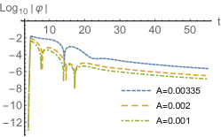
(a) $f_{1}=\varphi^{4}$

(b) $f_{2}=\varphi^{4}-\varphi^{6}$

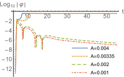
(c) $f_{3}=\varphi^{4}-\varphi^{8}$

Figure 1: Time evolution of the scalar field on the Schwarzschild background with $M=0.1,\lambda=1$, and $\Psi(t=0,r)=A\exp[-\frac{(r_{j}+1)^{2}}{1/5000}]$. The coupling functions of the left, middle and right graphs are given by $\varphi^{4},\varphi^{4}-\varphi^{6}$ and $\varphi^{4}-\varphi^{8}$, respectively.

III Numerical solutions of scalarized black holes

We wish to construct scalarized black hole solutions by solving the full equations (3)(4) numerically. The static and spherically symmetric black hole can be described by

$$d{s^{2}}=-{e^{2\xi(r)}}d{t^{2}}+{e^{2\Lambda(r)}}d{r^{2}}+{r^{2}}(d{\theta^{2}}+{\sin^{2}}\theta d{\phi^{2}}).$$ (17)

Substituting the metric ansatz (17) into Eqs. (3)(4), we obtain four equations

$$\frac{2}{r}\Big{[}{1+\frac{2}{r}(1-3{e^{-2\Lambda}}){\psi_{r}}}\Big{]}\frac{{d\Lambda}}{{dr}}+\frac{{{e^{2\Lambda}}-1}}{{{r^{2}}}}-\frac{4}{{{r^{2}}}}(1-{e^{-2\Lambda}})\frac{{d{\psi_{r}}}}{{dr}}-{\left({\frac{{d\varphi}}{{dr}}}\right)^{2}}=0,$$ (18)

$$\frac{2}{r}\left[{1+\frac{2}{r}(1-3{e^{-2\Lambda}}){\psi_{r}}}\right]\frac{{d\xi}}{{dr}}-\frac{{{e^{2\Lambda}}-1}}{{{r^{2}}}}-{\left({\frac{{d\varphi}}{{dr}}}\right)^{2}}=0,$$ (19)

$$\frac{{{d^{2}}\xi}}{{d{r^{2}}}}+\left({\frac{{d\xi}}{{dr}}+\frac{1}{r}}\right)\left({\frac{{d\xi}}{{dr}}-\frac{{d\Lambda}}{{dr}}}\right)+\frac{{4{e^{-2\Lambda}}}}{r}\left[{3\frac{{d\xi}}{{dr}}\frac{{d\Lambda}}{{dr}}-\frac{{{d^{2}}\xi}}{{d{r^{2}}}}-{{\left({\frac{{d\xi}}{{dr}}}\right)}^{2}}}\right]{\psi_{r}}$$

$$-\frac{{4{e^{-2\Lambda}}}}{r}\frac{{d\xi}}{{dr}}\frac{{d{\psi_{r}}}}{{dr}}+{\left({\frac{{d\varphi}}{{dr}}}\right)^{2}}=0,$$ (20)

$$\frac{{{d^{2}}\varphi}}{{d{r^{2}}}}+\left({\frac{{d\xi}}{{dr}}-\frac{{d\Lambda}}{{dr}}+\frac{2}{r}}\right)\frac{{d\varphi}}{{dr}}-\frac{{2{\lambda^{2}}}}{{{r^{2}}}}\frac{{df(\varphi)}}{{d\phi}}\Big{\{}{(1-e^{-2\Lambda})\left[{\frac{{d^{2}}\xi}{d{r^{2}}}+\frac{d\xi}{dr}\left({\frac{d\xi}{dr}-\frac{d\Lambda}{dr}}\right)}\right]+2{e^{-2\Lambda}}\frac{d\xi}{{dr}}\frac{d\Lambda}{dr}}\Big{\}}=0$$ (21)

with

$${\psi_{\rm{r}}}={\lambda^{2}}\frac{{df(\varphi)}}{{d\varphi}}\frac{{d\varphi}}{{dr}}.$$ (22)

Here we need to introduce the boundary conditions for this work. Our quest for asymptotically flat black hole solutions with a non-trivial scalar hair requires boundary conditions at asymptotic infinity and near the horizon:

$$\xi\left|{{}_{r\to\infty}\to 0,\quad\Lambda\left|{{}_{r\to\infty}}\right.}\right.\to 0,\quad\varphi\left|{{}_{r\to\infty}}\right.\to 0,$$

$${e^{2\xi}}\left|{{}_{r\to r_{h}}\to 0,}\quad\right.{e^{-2\Lambda}}\left|{{}_{r\to r_{h}}\to 0.}\right.$$ (23)

The mass of the black hole $M$ and scalar charge $D$ appear through the asymptotic forms of $\Lambda,\xi$, and $\varphi$ as Antoniou:2017acq

$${e^{2\xi}}= 1-\frac{{2M}}{r}+\frac{{{D^{2}}}}{{{r^{2}}}}+\frac{{3{D^{2}}M}}{{{r^{3}}}}+\frac{{-{D^{4}}+\frac{{16{D^{2}}{M^{2}}}}{3}}}{{{r^{4}}}}+\cdots,$$

$${e^{-2\Lambda}}= 1+\frac{{2M}}{r}+\frac{{-{D^{2}}+4{M^{2}}}}{{{r^{2}}}}+\frac{{-5{D^{2}}M+8{M^{3}}}}{{{r^{3}}}}+\frac{{{D^{4}}-16{D^{2}}{M^{2}}+16{M^{4}}}}{{{r^{4}}}}+\cdots,$$

$$\varphi= {\varphi_{\infty}}+\frac{D}{r}+\frac{{DM}}{{{r^{2}}}}-\frac{{D\left({{D^{2}}-8{M^{2}}}\right)}}{{6{r^{3}}}}+\cdots$$ (24)

with $\varphi_{\infty}=0$.

As stated in the previous section, we consider the relevant coupling function for obtaining scalarized black holes

$$f(\varphi)=\alpha({\varphi^{4}}-\beta{\varphi^{6}}),$$ (25)

where we set $\lambda=1$ because a coupling parameter $\alpha$ is included in $f(\varphi)$. We start by picking small parameters ($\alpha=1,\beta=1$) and the numerical results are shown in Fig. 2. The horizon radius is selected as $r_{h}=0.1$. This picture displays that the metric function gradually increases from zero at the horizon and approaches $1$ at infinity. This behavior is very similar to Schwarzschild solution. Enlarging the local results in Fig. 2(a), it is clear that $g_{tt}(r)$ and $g_{rr}(r)$ curves of scalarized black holes are below Schwarzschild solution $A(r)$. In Fig. 2(b), we introduce two differences between the scalarized and Schwarzschild metric functions defined by ${\Delta_{1}}(r)={e^{2\xi(r)}}-(1-\frac{{0.1}}{r})$ and ${\Delta_{2}}(r)={e^{-2\Lambda(r)}}-(1-\frac{{0.1}}{r})$. We find that these near the origin are greater than zero and are decreasing with two lowest points at $r=-0.002$ and $r=-0.0015$. Then, $\Delta_{1}$ and $\Delta_{2}$ increase but they remain below the $x$-axis. The scalar field decreases as $r$ increases and approaches $0$ as shown in Fig. 2(c). The above results imply that nonlinear scalarized black holes are similar to spontaneous scalarized black holes.

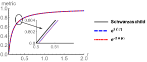
(a) Metric functions

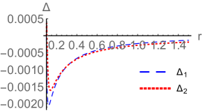
(b) Differences of two metric functions

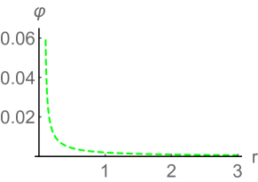
(c) Scalar hair

Figure 2: Metric functions and scalar field as functions of $r$. Here, we choose $\alpha=1,\beta=1$ and ${r_{h}}=0.1$.

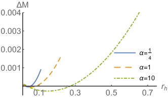
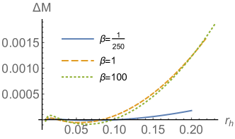
Figure 3: Mass as a function of horizon radius $r_{h}$ with $M_{0}=0.05$ mass of Schwarzschild black hole. In the left, $\beta=1,\alpha=\frac{1}{4},1,10$ and in the right, we choose $\alpha=1,\beta=\frac{1}{250},1,100$.

We further investigate the mass difference between scalarized and Schwarzschild black holes. We plot a figure for difference $\Delta M=M-M_{0}$ vs. horizon radius $r_{h}$ in Fig.3 , where $M$ and $M_{0}$ are the masses of scalarized and Schwarzschild black holes, respectively. In the left panel of Fig.3, we choose $\beta=1$. It turns out that $M-M_{0}$ decreases first and, then increases. With the increase of $\alpha$, the minimum value of $M-M_{0}$ decreases, while its maximum value increases significantly. In the right of Fig.3, we choose $\alpha=1$. Changing $\beta$, it shows a similar conclusion to the left panel. In addition, the smaller the $\beta$, the smoother the $M-M_{0}$ curve.

The connection between scalar field on the black hole horizon $r_{h}$ and mass $M$ is also worth exploring. These results are shown in Fig.4, where it illustrates the uniqueness of our model with the coupling function $f(\varphi)$ in Eq.(25). Obviously, the role of $\alpha$ is quite different from $\beta$ in making nonlinear scalarized black holes. The coupling parameter $\alpha$ plays a major role in making different nonlinear scalarized black holes, while the coupling parameter plays a supplementary role. We first fix $\beta$ and change $\alpha$, which is depicted in the left of the graph. This implies that $\varphi_{h}$ is a monotonically increasing function of $M$ (the same behavior with $r_{h}$). This implies that a non-linear parameter $\alpha$ affects the slope of this line: the larger the $\alpha$, the smaller the slope. However, this change have no effect on the maximum value of $\varphi_{h}$. In the right of the graph, we fix $\alpha$ first and change $\beta$. This result is contrary to the left of the graph, showing that changing $\beta$ hardly affects the slope of the $\varphi_{h}(M)$ line, but the maximum $\varphi_{h}$ increases as $\beta$ increases.

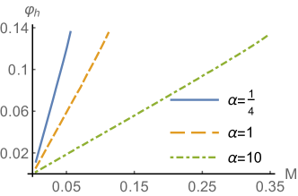
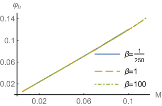
Figure 4: Scalar field at the event horizon as function of mass. In the left, $\alpha=\frac{1}{4},1,10.\beta=1$, while in the right, $\beta=\frac{1}{250},1,100$.

Also, Fig.5 shows the scalar charge $D$ as a function of the black hole mass $M$ and the effects of different $\alpha$ and $\beta$ on the scalar charge $D$ are clearly displayed. In the left panel with fixed $\beta=1$, $D$ shows increasing functions as $M$ increases. The value of $D$ increases curvilinearly as $M$ increases and eventually stops at the end point. The larger the value of $\alpha$, the larger the end point of $D$. In the right panel, we fix $\alpha=1$ first and change $\beta$. This result is contrary to the left of the graph, indicating that changing $\beta$ hardly affects the slope of the $D(M)$ curve, but the maximum $\varphi_{h}$ increases as $\beta$ increases. $D(M)$ curves show similar behaviors to $\varphi_{h}(M)$ for roles of $\alpha$ and $\beta$ in making different nonlinear scalarized black holes.

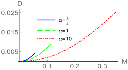
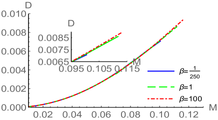
Figure 5: Scalar charge as a function of the black hole mass. In the left, $\beta=1,\alpha=\frac{1}{4},1,10$ and in the right, $\alpha=1,\beta=\frac{1}{250},1,100.$

.

Based on the numerical solutions we have obtained, we can further calculate the thermodynamic properties of these black holes. In static spherically symmetric black hole spacetime, the temperature takes the form

$$T=\frac{{\sqrt{{e^{\xi(r)}}^{\prime}({r_{h}})*{e^{\Lambda(r)}}^{\prime}({r_{h}})}}}{{4\pi}}.$$ (26)

It is interesting to study the profiles of the area of the black hole horizon, $A_{h}=4\pi{r_{h}}^{2}$ and of the entropy $S$ of this class of solutions Antoniou:2017hxj Gibbons:1976ue .

$${S}=\frac{1}{4}{A_{h}}+4\pi{\lambda^{2}}f({\varphi_{h}}).$$ (27)

As is shown in Fig.6, the entropy decreases as $\alpha$ increases for fixed $\beta=1$ and the entropy decreases as $\beta$ increases for fixed $\alpha=1$. Schwarzschild black hole lies on the top.

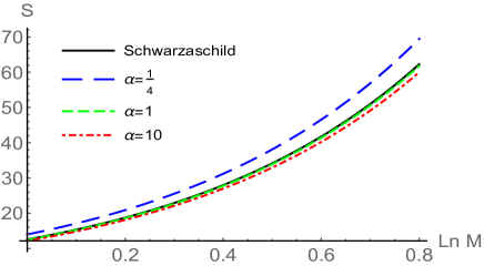
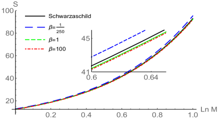
Figure 6: Black hole entropy as a function of mass. In the left, $\beta=1,\alpha=\frac{1}{4},1,10$ and in the right, $\alpha=1,\beta=\frac{1}{250},1,100$.

Now we discuss the first-law of thermodynamics of the hairy black holes. In order to evaluate this law, the discrete values of thermodynamic quantities of mass $M$, temperature $T$ and entropy $S$ with different horizon radius $r_{h}$ are shown in Table.1.

$No.$	$r_{h}$	$M$	$T$	$S$
1	0.01	0.004988	7.958000	0.005872
2	0.03	0.015004	2.652330	0.002829
3	0.05	0.024942	1.591190	0.007863
4	0.07	0.035000	1.136250	0.015430
5	0.09	0.045021	0.883451	0.025546
6	0.11	0.055063	0.722499	0.038237
7	0.13	0.065316	0.610955	0.053533
8	0.15	0.075491	0.529097	0.071477
9	0.17	0.085648	0.466433	0.092121
10	0.19	0.096001	0.416862	0.115541

Table 1: Mass $M$, temperature $T$, and entropy $S$ of scalarized black hole with different $r_{h}$ and $\alpha=\beta=1$.

Forward differences of mass $M$ entropy $S$ can be written as Zou:2019onm

$$\Delta M \equiv \frac{{M(i+2)-M(i)}}{2},$$

$$= \{0.019953,0.019996,0.020080,0.020064,0.020294,0.020428,$$

$$0.020333,0.020510,0.020802\},$$

$$\Delta S \equiv \frac{{S(i+2)-S(i)}}{2},$$ (28)

$$= \{0.007549,0.012601,0.017683,0.022807,0.027987,0.033240,$$

$$0.038588,0.044064,0.049746\}.$$

Then, the expression $dM=TdS$ in the form of discrete points is given by

$$\Delta M(i)-(T(i+1)\cdot\Delta S(i))$$ (29)

$$= \{-6.95*{10^{-5}},-5.53*{10^{-5}},-1.27*{10^{-5}},-8.52*{10^{-5}},7.37*{10^{-5}},$$

$$1.19*{10^{-4}},-8.42*{10^{-5}},-4.26*{10^{-5}},6.47*{10^{-5}}\}.$$

Thus, the thermodynamic quantities of the hairy black holes are seen to obey the first law $dM=TdS$ to quite a high precision.

IV Conclusions and discussions

We have discovered the existence of a fully nonlinear dynamical mechanism for forming scalarized black holes, which is different from the spontaneous scalarization. We considered three types of polynomial coupling functions satisfying $f^{\prime\prime}(0)=0$ for which the Schwarzschild black hole is still a linearly stable solution to the linearized equations. However, for certain ranges of the amplitude $A$ of a scalar field, scalarized black hole phases appear if the coupling function $f(\varphi)$ includes term higher than $\varphi^{6}$. This was shown by solving the non-linear scalar equation (13) in (1+1)dimensions numerically.

To obtain nonlinear scalarized black hole solutions, we select the most intuitive coupling function $\alpha(\varphi^{4}-\beta\varphi^{6})$ where the parameter $\alpha$ measures the overall effect of the scalar field on making nonlinear scalarized black hole, whereas the other $\beta$ represents the effect of higher order terms on making nonlinear scalarized black holes. We confirm the feasibility of our conjecture through calculation and analysis. Our numerical results have shown that scalarized black hole phases always exists for different coupling parameters $\alpha$ and $\beta$. It is important to note that the role of $\alpha$ is quite different from $\beta$ in making nonlinear scalarized black holes. The coupling parameter $\alpha$ plays a major role in making different nonlinear scalarized black holes, while the coupling parameter $\beta$ plays a supplementary role. This was shown by observing scalar hair at the horizon $\varphi(M)$ and scalar charge $D(M)$ for different $\alpha$ and $\beta$. This indicates that the nonlinear instability is a way of obtaining scalarized black holes, in addition to tachyonic instability for spontaneous scalarization.

Interestingly, we studied the thermodynamic properties of nonlinear scalarized black holes. We analyzed the relationship between black hole entropy $S$ and mass $M$ under different coupling parameters, and compare it with Schwarzschild black hole entropy. The entropy decreases as $\alpha$ increases for fixed $\beta=1$ as well as the entropy decreases as $\beta$ increases for fixed $\alpha=1$. The curve of Schwarzschild black hole lies on the top. Finally, we proved that the first-law of thermodynamics $dM=TdS$ is satisfied numerically for $\alpha=\beta=1$.

Acknowledgments

We appreciate Guo-Yang Fu for helpful discussion. D. C. Z is supported by National Natural Science Foundation of China (NSFC) (Grant No. 12365009) and Jiangxi Provincial Natural Science Foundation (No. 20232BAB201039). M. Y. L is supported by the National Natural Science Foundation of China with Grant No. 12305064 and Jiangxi Provincial Natural Science Foundation with Grant No. 20224BAB211020.

References

- (1) J. D. Bekenstein, “Exact solutions of Einstein conformal scalar equations,” Annals Phys. 82, 535 (1974).
- (2) J. D. Bekenstein, “Black Holes with Scalar Charge,” Annals Phys. 91, 75 (1975).
- (3) K. A. Bronnikov and Y. .N. Kireev, “Instability of Black Holes with Scalar Charge,” Phys. Lett. A 67, 95 (1978).
- (4) J. D. Bekenstein, “Novel “no-scalar-hair” theorem for black holes,” Phys. Rev. D 51 (1995) no.12, R6608
- (5) T. Damour and G. Esposito-Farese, “Nonperturbative strong field effects in tensor - scalar theories of gravitation,” Phys. Rev. Lett. 70 (1993), 2220-2223
- (6) D. D. Doneva and S. S. Yazadjiev, “New Gauss-Bonnet Black Holes with Curvature-Induced Scalarization in Extended Scalar-Tensor Theories,” Phys. Rev. Lett. 120, no.13, 131103 (2018) [arXiv:1711.01187 [gr-qc]].
- (7) H. O. Silva, J. Sakstein, L. Gualtieri, T. P. Sotiriou and E. Berti, “Spontaneous scalarization of black holes and compact stars from a Gauss-Bonnet coupling,” Phys. Rev. Lett. 120, no.13, 131104 (2018) [arXiv:1711.02080 [gr-qc]].
- (8) G. Antoniou, A. Bakopoulos and P. Kanti, “Evasion of No-Hair Theorems and Novel Black-Hole Solutions in Gauss-Bonnet Theories,” Phys. Rev. Lett. 120, no.13, 131102 (2018) [arXiv:1711.03390 [hep-th]].
- (9) G. Antoniou, A. Bakopoulos and P. Kanti, “Black-Hole Solutions with Scalar Hair in Einstein-Scalar-Gauss-Bonnet Theories,” Phys. Rev. D 97 (2018) no.8, 084037 [arXiv:1711.07431 [hep-th]].
- (10) Y. S. Myung and D. C. Zou, “Gregory-Laflamme instability of black hole in Einstein-scalar-Gauss-Bonnet theories,” Phys. Rev. D 98, no. 2, 024030 (2018) [arXiv:1805.05023 [gr-qc]].
- (11) H. O. Silva, C. F. B. Macedo, T. P. Sotiriou, L. Gualtieri, J. Sakstein and E. Berti, “Stability of scalarized black hole solutions in scalar-Gauss-Bonnet gravity,” Phys. Rev. D 99 (2019) no.6, 064011 [arXiv:1812.05590 [gr-qc]].
- (12) E. Berti, L. G. Collodel, B. Kleihaus and J. Kunz, “Spin-induced black-hole scalarization in Einstein-scalar-Gauss-Bonnet theory,” Phys. Rev. Lett. 126 (2021) no.1, 011104 [arXiv:2009.03905 [gr-qc]].
- (13) C. A. R. Herdeiro, E. Radu, N. Sanchis-Gual and J. A. Font, “Spontaneous Scalarization of Charged Black Holes,” Phys. Rev. Lett. 121, no.10, 101102 (2018) [arXiv:1806.05190 [gr-qc]].
- (14) P. G. S. Fernandes, C. A. R. Herdeiro, A. M. Pombo, E. Radu and N. Sanchis-Gual, “Spontaneous Scalarisation of Charged Black Holes: Coupling Dependence and Dynamical Features,” Class. Quant. Grav. 36 (2019) no.13, 134002 [erratum: Class. Quant. Grav. 37 (2020) no.4, 049501] [arXiv:1902.05079 [gr-qc]].
- (15) Y. S. Myung and D. C. Zou, “Instability of Reissner–Nordström black hole in Einstein-Maxwell-scalar theory,” Eur. Phys. J. C 79, no. 3, 273 (2019) [arXiv:1808.02609 [gr-qc]].
- (16) D. C. Zou and Y. S. Myung, “Radial perturbations of the scalarized black holes in Einstein-Maxwell-conformally coupled scalar theory,” Phys. Rev. D 102, no. 6, 064011 (2020) [arXiv:2005.06677 [gr-qc]].
- (17) Y. S. Myung and D. C. Zou, “Quasinormal modes of scalarized black holes in the Einstein–Maxwell–Scalar theory,” Phys. Lett. B 790 (2019), 400-407 [arXiv:1812.03604 [gr-qc]].
- (18) C. Promsiri, T. Tangphati, E. Hirunsirisawat and S. Ponglertsakul, “Scalarization of planar anti–de Sitter charged black holes in Einstein-Maxwell-scalar theory,” Phys. Rev. D 108 (2023) no.2, 024015 [arXiv:2302.04654 [gr-qc]].
- (19) D. D. Doneva and S. S. Yazadjiev, “Beyond the spontaneous scalarization: New fully nonlinear mechanism for the formation of scalarized black holes and its dynamical development,” Phys. Rev. D 105 (2022) no.4, L041502 [arXiv:2107.01738 [gr-qc]].
- (20) A. M. Pombo and D. D. Doneva, “Effects of mass and self-interaction on nonlinear scalarization of scalar-Gauss-Bonnet black holes,” Phys. Rev. D 108 (2023) no.12, 124068 [arXiv:2310.08638 [gr-qc]].
- (21) S. J. Zhang, “Nonlinear instability and scalar clouds of spherical exotic compact objects in scalar-Gauss-Bonnet theory,” Eur. Phys. J. C 83 (2023) no.10, 950 [arXiv:2304.08092 [gr-qc]].
- (22) J. L. Blázquez-Salcedo, D. D. Doneva, J. Kunz and S. S. Yazadjiev, “Radial perturbations of scalar-Gauss-Bonnet black holes beyond spontaneous scalarization,” Phys. Rev. D 105 (2022) no.12, 124005 [arXiv:2203.00709 [gr-qc]].
- (23) D. D. Doneva, L. G. Collodel and S. S. Yazadjiev, “Spontaneous nonlinear scalarization of Kerr black holes,” Phys. Rev. D 106 (2022) no.10, 104027 [arXiv:2208.02077 [gr-qc]].
- (24) M. Y. Lai, D. C. Zou, R. H. Yue and Y. S. Myung, “Nonlinearly scalarized rotating black holes in Einstein-scalar-Gauss-Bonnet theory,” Phys. Rev. D 108 (2023) no.8, 084007 [arXiv:2304.08012 [gr-qc]].
- (25) W. Xiong, C. Y. Zhang and P. C. Li, “The rotating solutions beyond the spontaneous scalarization in Einstein-Maxwell-scalar theory,” [arXiv:2312.11879 [gr-qc]].
- (26) G. W. Gibbons and S. W. Hawking, Phys. Rev. D 15 (1977), 2752-2756 doi:10.1103/PhysRevD.15.2752
- (27) D. C. Zou, C. Wu, M. Zhang and R. H. Yue, “Black holes in the Einstein-Born-Infeld-Weyl gravity,” EPL 128 (2019) no.4, 40006