Quantitative Results on Symplectic Barriers
Abstract
In this paper we present some quantitative results concerning symplectic barriers. In particular, we answer a question raised by Sackel, Song, Varolgunes, and Zhu regarding the symplectic size of the -dimensional Euclidean ball with a codimension-two linear subspace removed.
1 Introduction and Results
In a recent work [6], we established a new type of rigidity for symplectic embeddings that originates from obligatory intersections with symplectic submanifolds. Inspired by the terminology introduced by Biran [2] for analogous results regarding Lagrangian submanifolds, we refer to such symplectic obstructions as symplectic barriers. More precisely, if is a -dimensional symplectic manifold, a symplectic submanifold is said to be a symplectic barrier if
where is some (normalized) symplectic capacity. Recall that symplectic capacities are numerical invariants that, roughly speaking, measure the size of a symplectic manifold (see, e.g., Chapter 2 of [9]). More precisely,
Definition 1.1.
A symplectic capacity is a map which associates to every symplectic manifold an element of with the following properties:
-
•
if (Monotonicity)
-
•
for all , (Conformality)
-
•
(Nontriviality and Normalization)
Here denotes the -dimensional Euclidean ball with radius , denotes the cylinder , and stands for a symplectic embedding. Note that both the ball and the cylinder are equipped with the standard symplectic form on . Two examples of symplectic capacities, which naturally arise from Gromov’s celebrated non-squeezing theorem [5], are the Gromov width and the cylindrical capacity:
Another important example is the Hofer-Zhender capacity , which is closely related with Hamiltonian dynamics (see, e.g., [8]). It follows immediately from Definition 1.1 that for any symplectic capacity . For more information on symplectic capacities, see e.g., the survey [4].
In this paper we present some quantitative results concerning symplectic barriers. Our first result answers a question raised in Section 6.2 of [11] regarding the capacity of the -dimensional Euclidean ball in with a codimension-two linear subspace removed, where the classical Kähler angle is used to measure the “defect” of the subspace from being complex. More precisely, let be a codimension-two linear subspace with Kähler angle , i.e, the unit outer normals to satisfy . The following result shows that the -ball is a symplectic barrier in when .
Theorem 1.2.
Let and . For any symplectic capacity one has
We remark that the complex case follows from Proposition 1.6 in [6] (cf. Theorem 3.1.A in [10]). For the Gromov width, the Lagrangian case follows from [2], where it is proved that . Moreover, one can check that Theorem 1.3 in [11] implies that .
Our next result concerns the symplectic barriers introduced in [6]. For denote by the following union of symplectic codimension-two subspaces in :
Moreover, define to be a linear image of such that the Kähler angle of the corresponding planes is , i.e., , where are the unit outer normals to the subspaces in . Note that any two such configurations of subspaces with the same Kähler angle are unitarily equivalent. We also note that when is sufficiently large, the intersection becomes , where is a single codimension-two subspace of Kähler angle as above. Thus we are especially interested in the case when is small. In [6] it was proved that for small , the configurations are symplectic barriers of the ball with respect to any (normalized) symplectic capacity. Here we provide more precise bounds for the symplectic size of the complement of in when .
Theorem 1.3.
For any and
We suspect that Theorem 1.3 also holds for the Gromov width. This is supported by the following claim that provides an almost exact lower bound:
Theorem 1.4.
While Theorem 1.2 shows that the complement of a single codimension-two linear subspace with Kähler angle has capacity , the two theorems above show that the symplectic size of the complement of a large number of such spaces is strictly smaller, and takes a value around the Kähler angle .
Acknowledgements: We are grateful to Yael Karshon for numerous enlightening discussions, particularly for her generous sharing of ideas concerning the proof of Proposition 3.3, which is crucial for the results in Section 3. P. H-K. and Y.O. were partially supported by the ISF grant No. 938/22, and R.H. by the Simons Foundation grant No. 663715.
2 The Complement of a Single Subspace
In this section we prove Theorem 1.2. We first introduce the following notations. Equip with coordinates , where , and with the standard symplectic form . Let be the real two-dimensional plane in spanned by the two vectors and , where are positive real numbers satisfying . It is not hard to check that using a linear unitary transformation in , we can assume without loss of generality that any codimension-two linear space with Kähler angle is of the form . This implies that the proof of Theorem 1.2 is, roughly speaking, four-dimensional.
The strategy for the proof of Theorem 1.2 is as follows: first we prove the required lower bound for the Gromov width by an explicit embedding of a 4-dimensional ball in (Proposition 2.2), and then extend the argument to any dimension in Proposition 2.3. Next, in Proposition 2.4 we develop the main ingredient needed for the required upper bound for the cylindrical capacity, which in turn is proved in Proposition 2.12.
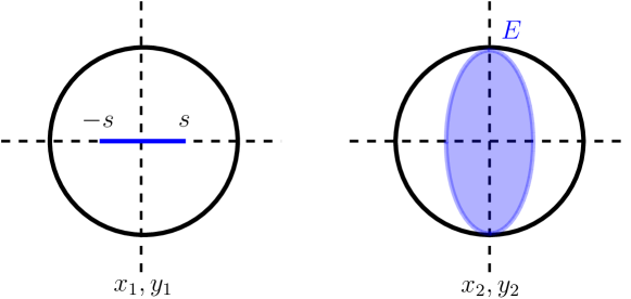
We start with some preparation. First, note that the plane lies in the hyperplane . Moreover, let be the projection onto the -plane, for . Then, one has
where is the ellipse with axes , , and area (see Figure 1).
Set , , , and . Note that any subset of the intersection satisfying can be displaced from using a Hamiltonian diffeomorphism of that sends points of the form to , with . This can be done, e.g., via the following simple lemma.
Lemma 2.1.
Let be a submanifold and let be a vector field on tangent to whose time- flow defines a diffeomorphism of . Then there exists a Hamiltonian diffeomorphism of which preserves and restricts to on .
Proof.
As the -form vanishes on , one can find a function which vanishes on , and satisfies . Clearly the function generates the required Hamiltonian diffeomorphism. ∎
With these preliminaries in place, we turn now to prove the required lower bound for the Gromov width in dimension four.
Proposition 2.2.
For any one has,
Proof.
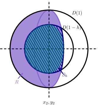
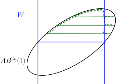
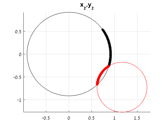
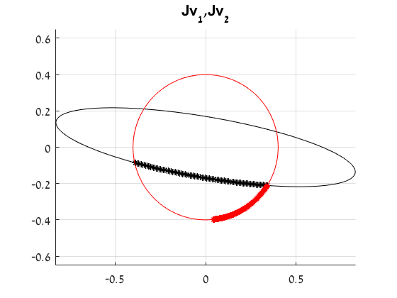
By the remark proceeding Lemma 2.1, for the proof of the proposition it suffices to find a symplectic embedding with image satisfying . Denote by the disk of area centered at the origin. Note that divides the disc into two regions, and set to be the one with area . Next, let (see Figure 2). Note that is the set of all points in such that the fibers of the map in have area at least . It is not hard to check that the area of is at least . Indeed, the area of is , while the area of can be bounded from below by half the area of an ellipse centered at the origin with radii and , where and .
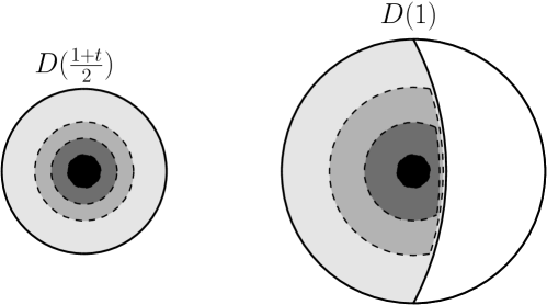
We shall construct an area preserving map from to , such that the product is the required symplectic embedding . Note that the image if for all . Indeed, let such that and for some . If , then, as , one as . Using Lemma 3.1.5 in [12] (see Figure 3), one can construct such a map since
for all . Finally, as the -component of lies in , such a map automatically satisfies , as required. This completes the proof of the proposition. ∎
We can extend Proposition 2.2 to higher dimensions as follows.
Proposition 2.3.
For any and
Proof.
We would like to construct a Hamiltonian function whose corresponding time- flow maps the ball into . From the proof of Proposition 2.2 it follows that there exists a Hamiltonian function whose time- flow maps the ball into . It follows that for every the time-1 map of the Hamiltonian function maps into . Next, for a point , set . Note that . Hence, since , the time- map of the Hamiltonian function
satisfies
as required (cf. [3], Section 2.1). This completes the proof of the proposition. ∎
Next we turn to establish the upper bound in Theorem 1.2. For this, let be the Lagrangian plane spanned by and . Note that both and lie in the hyperplane , and one has . The main ingredient we need is the following:
Theorem 2.4.
Let be a compact subset. Then there exists a symplectomorphism of with .
Proof.
Set with , defined as follows:
Since is a graph over the -plane, is the disjoint union of and . Further, since are positive we have that and This implies in particular that and . Indeed, for , if , then , and then . Hence . A similar argument holds for points in .
Our proof has two steps. In Step 1 we apply a symplectic diffeomorphism to , with support in , moving first the subsets and away from , and then moving sufficiently away from the -axis. In Step 2 we describe a Hamiltonian diffeomorphism of displacing the re-positioned obtained in Step 1 from as required.
Step 1. The repositioning of is achieved via the following two lemmas.
Lemma 2.5.
For every sufficiently small, there exists a Hamiltonian diffeomorphism with compact support in such that the sets and defined for satisfy and .
Proof.
We can find such a diffeomorphism which preserves by applying Lemma 2.1, since moving points of in the positive -direction, and points of in the negative -direction does not introduce intersections with . ∎
To simplify notations, in what follows we denote the image provided by Lemma 2.5 also by .
Lemma 2.6.
For every sufficiently small there is a symplectic diffeomorphism which is the identity on , and satisfies
Proof.
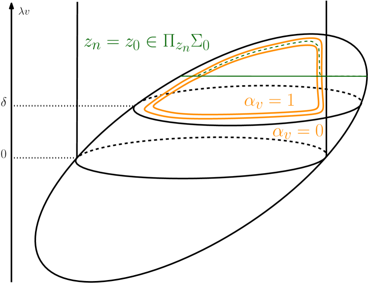
We use symplectic polar coordinates on the -plane, with and . Let satisfy when both and , and when or . Then, consider the closed -form . As is disjoint from , the form defines a symplectic isotopy of increasing the coordinate by and preserving . As , the ball remains disjoint from but stays within , as required (see Figure 4). This completes the proof of the lemma. ∎
Step 2. Displacing the repositioned from .
To further simplify notations, using Step 1, in what follows we assume that for some sufficiently small . In addition, note that , where and . Our goal is to find a Hamiltonian diffeomorphism of which displaces from . We must consider both and , and give sufficient conditions for a Hamiltonian function to generate a diffeomorphism displacing from , while leaving disjoint from . The proof will conclude by showing that Hamiltonian functions satisfying the sufficient conditions exist.
Displacing from .
We can find two Hamiltonian functions and , with compact support in whose corresponding time-1 flows, denoted by and respectively, satisfy and . This is because and are compact subsets of and , respectively, and both sets have area . In fact, as and are compact, choosing smaller if necessary we may assume and have compact support in . Note that one can choose such that . In addition, we can let on , and make sure the flow of remains in .
Next, let be such that if , if , and . We consider the Hamiltonian function defined by
| (1) |
Note that the Hamiltonian flow satisfies . More generally we have the following.
Lemma 2.7.
Suppose satisfies in and in a neighborhood of . Then the time-1 flow satisfies .
Proof.
Suppose (the argument for points in is identical), then . The component of the Hamiltonian vector field in the direction is given by , which vanishes when as agrees with . Also, as , when we have . Therefore the flow of remains in , and as the -component of on is independent of , we see that also displaces from . ∎
Controlling the flow of .
Note that showing that remains disjoint from under a Hamiltonian flow is equivalent to showing that the inverse flow applied to remains disjoint from . Consider the Hamiltonian flow generated by , so . This flow has the following property:
Lemma 2.8.
Let . With the above notations one has
Proof.
Suppose . Then we have
For a point , set to be its image under the flow of . Note that if , then and in particular . Assume . Note that if the projection , then by our assumption on the Hamlitonian function one has , and thus , i.e., . If , then, by the assumptions on and , one has that , and that . This completes the proof of the lemma for . A similar argument works for the case . ∎
Let be a symplectomorphism of the -plane mapping the region
into the disk . Furthermore, suppose that is the identity near . Define by . The following is a corollary of Lemma 2.8.
Corollary 2.9.
Let . Then
Proof.
The proof follows immediately from Lemma 2.8 and the fact that the flow of is given by . ∎
Our repositioning Lemma 2.6 now implies that . Slightly more generally, let be a neighborhood of the union of the sets for . Then we have the following.
Corollary 2.10.
Let so that on . Then .
Displacing .
Recall that the flow generated by a Hamiltonian function preserves the ball provided it is constant on the characteristic circles in . Summarizing our discussion above, combining Lemma 2.7. Corollary 2.10, and the symplectomorphism from Step 1, give the following.
Corollary 2.11.
Suppose is such that
-
1.
is constant on characteristics of ,
-
2.
in and in a neighborhood of ,
-
3.
on .
Then, the time-1 map restricts to give a diffeomorphism of which displaces from .
It remains to show that such functions exist. We will show that the three conditions in Corollary 2.11 are consistent.
We start by showing the compatibility of the first two conditions. For this we need to show that for each Hopf circle on , the restriction of to the intersection of the Hopf circle with , and to a neighborhood of , is constant.
Note that there is a single characteristic, , lying entirely in . As our functions and have compact support in , the function is identically on this circle. The remaining characteristics intersect in exactly two points, say and . Assume (a similar argument holds for ), note that
and so for each Hopf circle is constant on its intersection with . Thus can be extended over to a function constant on the characteristics.
Now we consider characteristics intersecting the neighborhood of . These characteristics intersect inside the region
where is identically . Hence a function on which agrees with on and is constant on characteristics will be identically on . In particular agrees with on a neighborhood of and we have shown the compatibility of conditions 1 and 2.
Regarding condition 3, as is relatively compact in the ball, its only intersection with the boundary is on . Also in a neighborhood of . Thus we can define a smooth function simultaneously equal to on , equal to on and in a neighborhood of , and equal to our extension of over which is constant on the characteristics. In other words, one can find a smooth function as required. This completes the proof of Theorem 2.4. ∎
Proposition 2.12.
For any and
Proof.
We need to produce a symplectic embedding
for all . Given a compact , Theorem 2.4 gives a symplectic embedding . Theorem 1.3 from [11] says that there exists a symplectic embedding , and so composing gives an embedding . Next we observe that embeds into a compact subset of for all . Indeed, a suitable embedding is the restriction of a symplectic embedding of into itself defined as follows. Write , where is the symplectic complement of . Let be a -small symplectic embedding , where is small neighborhood of the origin. Thus, the required embedding is
Compose the above embedding with , we obtain an embedding
To conclude, we observe that
satisfies
This completes the proof of the proposition. ∎
3 The Complement of Parallel Subspaces
In this section we prove Theorem 1.3 and Theorem 1.4. As before, assume that and equip with coordinates , and with the standard symplectic form .
The proof of Theorem 1.3 is broken into two parts: obtaining an upper bound for the cylindrical capacity, and a lower bound for the Hofer-Zehnder capacity. For the upper bound we need the following observation. Let be a convex body, and denote by the Ekeland-Hofer-Zehder capacity associated with , i.e., the minimal action among the closed characteristics on the boundary (see, e.g., Section 1.5 in [8]). Moreover, for , let be the linear map that takes to , and leaves fixed for .
Proposition 3.1.
For convex such that one has
Note that , and hence its capacity is taken with respect to the standard symplectic form restricted to .
Proof.
Assume without loss of generality that is also strictly convex and smooth. Recall that, by Clarke’s dual action principle (see, e.g., Section 1.5 of [9]), one has that for every convex body
| (2) |
where , the function is the support function of defined by , and is the symplectic action of . Moreover, one has that for , a minimizer of (2), and some and , the orbit is a closed characteristic on the boundary of with minimal action. Denote by a minimizer of (2) for the body , and by the corresponding closed characteristic. In order to bound the capacity of , we consider the loop defined by
where is the unit outer normal to at a point. Recall that as one has that can be assumed to be centrally symmetric (see Corollary 2.2. in [1]), and hence is a closed loop. Define and so that
Note that since ,
Moreover, since for every one has that ,
Next, since is parallel to , one has
This together with the definition of the support function implies that
Note that one has , where . As is bounded, one gets that as . Using (2) and normalizing appropriately, complete the proof. ∎
Recall that is a linear image of the set of codimension-two subspaces
| (3) |
with Kähler angle , i.e., one has , where are the unit outer normals to the subspaces in .
Proposition 3.2.
For any and , there exists such that
Proof.
Let , and consider the symplectic matrix (cf. Example 2.2. in [6])
It follows from the proof of Theorem 1.3 in [6] that for every
where , and is the family of complex planes (3). Since is a centrally symmetric ellipsoid, Proposition 3.1 implies that for every (normalized) symplectic capacity one has
A direct computation shows that is linearly symplectomorphic to the symplectic ellipsoid which has capacity . Note that the normals to (in the -coordinate system) are
and hence . Overall, for any and , there exist and such that
and the proof of the proposition is thus complete. ∎
We turn now to obtain the required lower bound for the Hofer-Zehnder capacity. To this end we shall need the following
Proposition 3.3.
Let and , and let be a symplecitc matrix such that . Then for every there is a symplectic embedding
where
Proof.
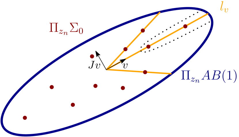
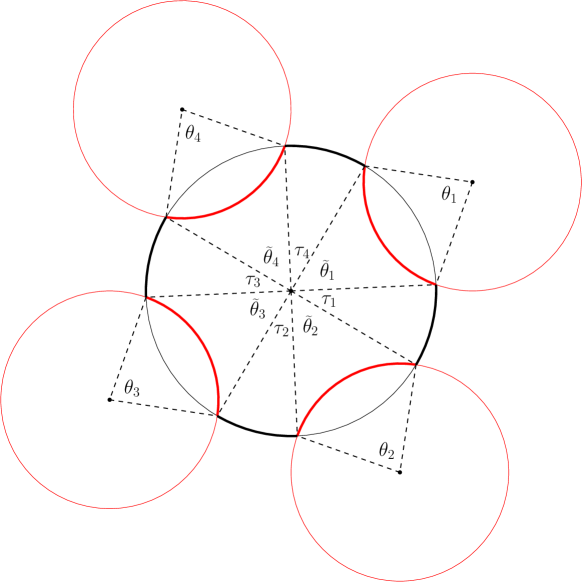
The idea of the proof is to “push” to a small neighborhood of the boundary of via a symplectic isotopy (see Figure 5). Then, will give the required embedding. More precisely, let be the set of all the directions connecting points in to the origin. For every , set such that cover all the points in (see Figure 7). Next, consider
and define a function such that it vanishes outside , is equal to in the interior of , and with some smooth cut-off in between (see Figure 7). Define a smooth function such that it equals in a small neighborhood of , and vanishes outside a slightly larger neighborhood (by choosing the former neighborhood small enough, one can make sure that the supports of are disjoint). Note that the Hamiltonian vector field is equal to for such that and . Hence, the Hamiltonian function generates the required flow. Note that in a similar way one can also push the codimension-two hyperplane passing through the origin in to the boundary of . This completes the proof of the lemma. ∎
From Proposition 3.3 it follows that in order to obtain a lower bound for the capacity of it is enough to find a lower bound for the capacity of the intersection , which is a convex domain in . We will show below that the minimal action capacity of this domain equals , which is suffices for the proof of Theorem 1.3.
Remark 3.4.
In light of the well-known conjecture that all symplectic capacities coincide on convex domains in the classical phase space, one expects that the Gromov width of the intersection also equals . This, in turn, would imply that Theorem 1.3 holds for the Gromov width as well. However, we are only able to show that the Gromov width of the above intersection is bounded below by as stated in Theorem 1.4.
Proposition 3.5.
With the above notations one has
Proof.
We start with the 4-dimensional case. Based on the definition of the Ekeland-Hofer-Zehnder capacity and the fact that is a symplectic matrix, it suffices to show that any closed characteristic with minimal action on the boundary of has action . For this end, without loss of generality, one can choose to be the matrix
| (8) |
In this case the base of the cylinder is spanned by
Complete into an orthonormal basis with
Denote and , and note that . We classify the closed characteristics on the boundary by how many time they “visit” the sets and . More precisely, note that a closed characteristic which lies entirely in has action , and a closed characteristic which is entirely in has action . Moreover, such a characteristic in exists in the subspace spanned by . The other options include closed characteristics that pass between and and vice versa (maybe several times), and closed characteristics that stay in the intersection for all time. We analyse the latter two options below. We remark that from the proof below it follows that any closed characteristic spending a non-discrete time in must remain within this intersection indefinitely.
We start with some general observations regarding the Reeb dynamics that will be useful later on. Observe that the characteristics in are moving along two centred circles in the and -coordinate planes respectively, in the same direction and the same angular speed. The sum of the areas enclosed by the two circles is . On the other hand, a direct computation shows that the characteristics in are moving along two non-centred circles in the , -coordinate planes respectively, in opposite directions, and with the same angular speed. The areas enclosed by these circles are and , respectively.
Using the fact that if and only if
one can write
Note that for a point , the (not normalized) outer normal equals , and the characteristic direction is . On the other hand, for , the characteristic direction is , where
is the outer normal to at . From now on we set for a point so that
Moreover, a point in can be written as , where . One can check that
A direct computation shows that the projection of a Hopf circle passing through a point on the plane spanned by is an ellipse with area given by . Denote the projection of the Hopf circle on by , and the projection to the plane by . Denote the projection of the characteristics of on by (non-centred circles) and the projection on the plane spanned by by (centred circle of radius ).
We analyse first closed characteristics entirely contained in the intersection of and . Note that for the characteristic direction is a non-negative linear combination of the two outer normals and , denoted by for some . In order for the characteristic to stay in the intersection, needs to be tangent to , meaning , which is equivalent to . This condition, together with the fact that , implies that
We start with the case . In order for the characteristic to remain in the intersection one also needs to require that , and . This condition implies that , i.e. the velocity is only “coming” from . The point in Euclidean coordinates is of the form
and in this case . This is the same closed characteristic as in the case when the characteristic is contained in , which has action . In addition, we claim that moving in the direction of the Hopf circle (and possibly leaving the intersection) is not possible. Indeed, recall that the projection of the Hopf circle passing through is an ellipse, which is tangent to , a circle of radius (and area ). As the area of the ellipse is , it must contain the circle, and hence the Hopf circle intersects only in the tangency points. This observation also implies that a characteristic cannot get to from .
We turn to case that . The conditions and imply that . As , we get that this case holds only for . In this case,
This creates a simultaneous circular movement in the and planes. One can check that the projection of this orbit to the coordinates are also centred circles (rotating in opposite directions). The point in Euclidean coordinates is of the form
The symplectic action is thus
Since , the action is larger then . Similarly to the case of , the projection of the Hopf circle, , is an ellipse of area , which is larger than (as ). Hence the ellipse is tangent to the circle of radius from the outside, which means that the direction of the Hopf circle does not interact with this characteristic.
It remains to consider the case of a characteristic which alternates between and . Assume without loss of generality that the starting point of the characteristic is in and it moves along until it hits again the intersection. We claim that the norms of the and coordinates are the same at these two points (before and after moving in ). To show this, we calculate the intersection of a characteristic of with the boundary of the unit ball. Recall that a possible representation of this characteristic is
for fixed and . In Euclidean coordinates this becomes
This implies that
In the intersection , and hence
Since these expressions are independent of , we get that , for , is the same before and after the movement in . In addition, we note that as one varies and , the change in and is the same. Since , this means that the movement along lies inside the disc enclosed by . We continue along movement on , which has the same projection to as . Consider a closed characteristic which starts with movement in with angular change along , then movement on with angular change (see Figure 10), continuing with movements that alternate between and with angular movements . Denote by the angular change along which corresponds to .
As the radius of (i.e., ) is always smaller then the radius of (i.e., ), we get that . Hence the action of the loop is
where the last inequality is due to the fact that the loop is closed and the orientation of the loops does not change. This completes the proof of the proposition in the 4-dimensional case. For a general dimension , note that one can assume that the symplectic matrix, which we now denote by to distinguish it from the 4-dimensional case above, is of the form
where is the matrix (8). In this case one has
where stands for the symplectic -product defined more generally for two convex domains and by
From Proposition 1.5 in [7] one has
which completes the proof of the proposition. ∎
Proof of Theorem 1.3.
We turn now to the proof of Theorem 1.4, which shows, roughly speaking, that the Gromov width of is bounded below by an almost linear function.
Proof of Theorem 1.4.
From Proposition 3.3 it follows that it is enough to show that
where is a symplectic matrix such that . We may assume without loss of generality that the outer normals to the hyperplanes in are given by and , written here in the -coordinate system. Note that as symplectic matrix that maps to one can now take
We first describe two immediate bounds for . The first comes from the largest Euclidean ball contained in the domain . More precisely, let be the linear subspace such that and . Note that
and the corresponding symplectic orthogonal subspace is
In addition, the orthogonal complement of is
and since the orthogonal projection of to is
one has , which gives .
The second lower bound is provided by the largest Euclidean ball inside . More precisely, note that is of the form
which is a -dimensional symplectic ellipsoid containing the ball of capacity . On the other hand, for the largest ball inside one has
Thus, , which gives .
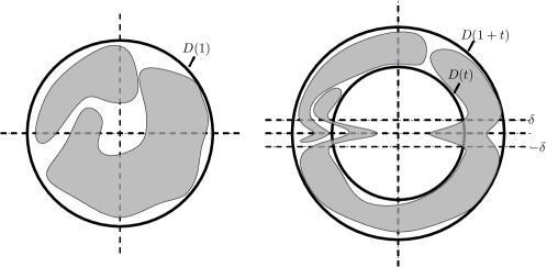
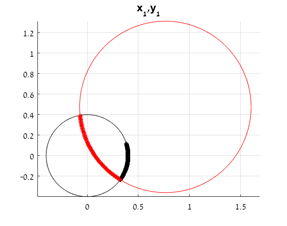
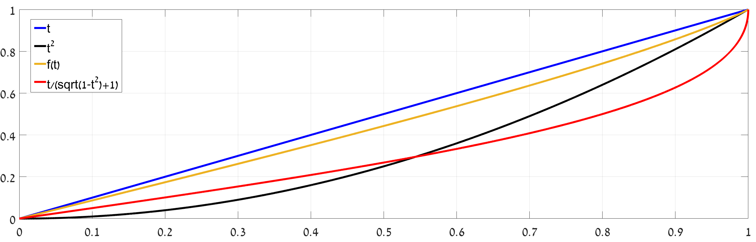
Note that none of the above bounds dominates the other (see Figure 11). Moreover, in the first case the constraint for embedding is coming from the intersection of the ball with the cylinder , while in the second case, the constraint is due to the intersection of a ball with . A way to improve the two bounds above is to consider a symplectic linear image of the ball such that the largest for which it fits in the ball is equal to the largest for which the image fits in the cylinder . For this, consider the following symplectic matrix for some parameters ,
Note that when this corresponds to the first embedding described above, and up to a unitary transformation (which does not change the embedding of the ball), there exist and which correspond to the second embedding, i.e., has this form after multiplying with a unitary matrix. Now we choose the parameters and such that the projection of the image of the ball to is a symplectic ellipsoid, or, in other words, that the base of the relevant symplectic image of the cylinder is always a disc. Moreover, as is often the case with similar optimization problems, we require that:
These two assumptions determine and , and when plugging these solutions into we conclude that one can fit into a ball of capacity
∎
Remark 3.6.
Numerical tests suggest that the embedding above of a ball with capacity given by is the best embedding one can find using only linear symplectic maps.
References
- [1] A. Akopyan, R. Karasev. Estimating symplectic capacities from lengths of closed curves on the unit spheres, arXiv:1801.00242.
- [2] P. Biran. Lagrangian barriers and symplectic embeddings, Geom. Funct. Anal., 11 (2001), 407–464.
- [3] O. Buse and R. Hind, Symplectic embeddings of ellipsoids in dimension greater than four, Geom. Topol. 15 (2011), 2091–2110.
- [4] Cieliebak, K., Hofer, H., Latschev, J., Schlenk, F. Quantitative symplectic geometry, in Recent Progress in Dynamics. Math. Sci. Res. Inst. Publ., 54 Cambridge University Press, Cambridge, 2007, 1–44.
- [5] Gromov, M. Pseudo holomorphic curves in symplectic manifolds, Invent. Math., 82 (1985), 307–347.
- [6] P. Haim-Kislev, R. Hind, Y. Ostrover. On the existence of symplectic barriers, Preprint. arXiv:2301.01822.
- [7] P. Haim-Kislev, Y. Ostrover. Remarks on symplectic capacities of -products, Internat. J. Math. 34 (2023), no. 4, Paper No. 2350021.
- [8] H. Hofer and E. Zehnder, A new capacity for symplectic manifolds, Analysis, et cetera, Academic Press, Boston, MA, 1990, pp. 405–427, 2011.
- [9] H. Hofer and E. Zehnder, Symplectic invariants and Hamiltonian dynamics, Birkhäuser Verlag, Basel, 1994.
- [10] D. McDuff, L. Polterovich. Symplectic packings and algebraic geometry. With an appendix by Yael Karshon, Invent. Math. 115(3) (1994), 405–434.
- [11] K. Sackel, A. Song, U. Varolgunes, and J. Zhu J. On certain quantifications of Gromov’s non-squeezing theorem. With an appendix by Joé Brendel, to appear in Geometry and Topology. arXiv:2105.00586.
- [12] F. Schlenk, Embedding problems in symplectic geometry, De Gruyter Expositions in Mathematics 40. Walter de Gruyter Verlag, Berlin, 2005.
Pazit Haim-Kislev
School of Mathematical Sciences, Tel Aviv University, Israel
e-mail: pazithaim@mail.tau.ac.il
Richard Hind
Department of Mathematics, University of Notre Dame, IN, USA.
e-mail: hind.1@nd.edu
Yaron Ostrover
School of Mathematical Sciences, Tel Aviv University, Israel
e-mail: ostrover@tauex.tau.ac.il