Convergence analysis of the transformed gradient projection algorithms on compact matrix manifolds

Abstract.

In this paper, to address the optimization problem on a compact matrix manifold, we introduce a novel algorithmic framework called the Transformed Gradient Projection (TGP) algorithm, using the projection onto this compact matrix manifold. Compared with the existing algorithms, the key innovation in our approach lies in the utilization of a new class of search directions and various stepsizes, including the Armijo, nonmonotone Armijo, and fixed stepsizes, to guide the selection of the next iterate. Our framework offers flexibility by encompassing the classical gradient projection algorithms as special cases, and intersecting the retraction-based line-search algorithms. Notably, our focus is on the Stiefel or Grassmann manifold, revealing that many existing algorithms in the literature can be seen as specific instances within our proposed framework, and this algorithmic framework also induces several new special cases. Then, we conduct a thorough exploration of the convergence properties of these algorithms, considering various search directions and stepsizes. To achieve this, we extensively analyze the geometric properties of the projection onto compact matrix manifolds, allowing us to extend classical inequalities related to retractions from the literature. Building upon these insights, we establish the weak convergence, convergence rate, and global convergence of TGP algorithms under three distinct stepsizes. In cases where the compact matrix manifold is the Stiefel or Grassmann manifold, our convergence results either encompass or surpass those found in the literature. Finally, through a series of numerical experiments, we observe that the TGP algorithms, owing to their increased flexibility in choosing search directions, outperform classical gradient projection and retraction-based line-search algorithms in several scenarios.

1. Introduction

1.1. Problem formulation

Let $\mathcal{M}\subseteq\mathbb{R}^{n\times r}$ be a compact matrix submanifold of class $C^{3}$ with $1\leq r\leq n$. In this paper, we mainly consider the following optimization problem:

$$\min_{\boldsymbol{X}\in\mathcal{M}}f(\boldsymbol{X}),$$ (1)

where the cost function $f$ is assumed to be twice continuously differentiable over $\mathbb{R}^{n\times r}$. Problem (1) has a wide range of applications in various fields, including signal processing [3, 24, 48], machine learning [41, 9, 79], numerical linear algebra [64, 65] and data analysis [5, 22, 42, 70].

In this paper, as two significant examples of the above problem (1), we mainly focus on the Stiefel manifold [28, 82] and the Grassmann manifold [12]. In fact, it is worth noting that the proposed algorithms and convergence results of this paper also apply to other compact matrix manifolds as well, e.g., the oblique manifold [75] and the product of Stiefel manifolds [36, 48], although we do not dive into the details in this paper. The Stiefel manifold is defined as $\mathbf{St}(r,n)\stackrel{{\scriptstyle\sf def}}{{=}}\{\boldsymbol{X}\in\mathbb{R}^{n\times r}:\boldsymbol{X}^{{\sf T}}\boldsymbol{X}=\boldsymbol{I}_{r}\}$ [73]. If $r=1$, it is the unit sphere $\mathbb{S}^{n-1}\subseteq\mathbb{R}^{n}$, and when $r=n$, it becomes the $n$-dimensional orthogonal group $\mathbf{O}_{n}\subseteq\mathbb{R}^{n\times n}$. The Grassmann manifold is defined as $\mathbf{Gr}(p,n)\stackrel{{\scriptstyle\sf def}}{{=}}\{\boldsymbol{X}\in\mathbb{R}^{n\times n}:\boldsymbol{X}^{{\sf T}}=\boldsymbol{X},\boldsymbol{X}^{2}=\boldsymbol{X},\mathop{\operator@font rank}(\boldsymbol{X})=p\}$ [10], which is a set of projection matrices satisfying $\mathop{\operator@font rank}(\boldsymbol{X})=p$. It is also isomorphic to $\mathbf{St}(p,n)/\mathbf{O}_{p}$, the quotient manifold of $\mathbf{St}(p,n)$ and $\mathbf{O}_{p}$ [12].

A diverse range of algorithms have been developed to address problem (1) in the literature, including both infeasible and feasible approaches. Infeasible methods encompass techniques such as the splitting methods [44], and penalty methods [83, 84, 81]. Feasible methods mainly include two classes. The first class stems from exploiting the geometric structure of $\mathcal{M}$, allowing for the direct implementation of various Riemannian optimization algorithms by making use of differential-geometric principles like geodesic and retraction; see e.g. [3, 17, 35]. The second class of feasible methods ensures that iterations consistently remain within the manifold by using the projection onto compact matrix manifolds.

1.2. Retraction-based line-search algorithms

A fundamental concept in the theory of differential manifold is the geodesic [55], which, in essence, embodies a locally shortest path on the manifold, offering a generalization of straight lines in Euclidean space [27, 29]. Meanwhile, in classical unconstrained optimization, a thoroughly examined class of line-search algorithms explores along straight lines in each iteration [55]. Therefore, it is natural to extend these classical line-search methods to manifolds through the utilization of geodesics. These types of algorithms have been extensively studied in early works; see [55, 29, 72, 85] and the references therein. It is worth noting that the algorithms proposed therein usually presume the explicit calculation of geodesics along a given direction.

While closed-form expressions of geodesics are available only for certain manifolds [28, 71], the computation of geodesics can be computationally expensive or even impractical in general, as shown in [16, 4]. To address this challenge, it has been suggested to approximate exact geodesics using computationally efficient alternatives [16, 31]. For example, in the context of the Stiefel manifold, various specially designed curves along search directions have been constructed with low computational cost, and curvilinear search algorithms have subsequently been developed based on these curves [82, 80, 40].

Note that geodesics can often be computed through an exponential map [28]. To approximate these geodesics effectively, it suffices to find an approximation of the exponential map, which gives rise to the concept of retraction [3, 69]. Let $\mathcal{M}^{\prime}\subseteq\mathbb{R}^{m}$ be a submanifold. A smooth map $\operatorname{R}$ from the tangent bundle $\mathbf{T}{\mathcal{M}^{\prime}}$ to $\mathcal{M}^{\prime}$ is said to be a retraction on $\mathcal{M}^{\prime}$ if it satisfies the following properties:

• $\operatorname{R}(\boldsymbol{x},\boldsymbol{0}_{\boldsymbol{x}})=\boldsymbol{x}$ for all $\boldsymbol{x}\in\mathcal{M}^{\prime}$, where $\boldsymbol{0}_{\boldsymbol{x}}$ denotes the zero element in the tangent space $\mathbf{T}_{\boldsymbol{x}}{\mathcal{M}^{\prime}}$;

• The differential of $\operatorname{R}_{\boldsymbol{x}}$ at $\boldsymbol{0}_{\boldsymbol{x}}$ is the identity map on $\mathbf{T}_{\boldsymbol{x}}{\mathcal{M}^{\prime}}$. Here $\operatorname{R}_{\boldsymbol{x}}:\mathbf{T}_{\boldsymbol{x}}{\mathcal{M}^{\prime}}\to\mathcal{M}^{\prime}$ denotes the restriction of $\operatorname{R}$ to $\mathbf{T}_{\boldsymbol{x}}{\mathcal{M}^{\prime}}$, i.e., $\operatorname{R}_{\boldsymbol{x}}(\cdot)\stackrel{{\scriptstyle\sf def}}{{=}}\operatorname{R}(\boldsymbol{x},\cdot)$.

Define a curve $c(t)$ on $\mathcal{M}^{\prime}$ passing through $\boldsymbol{x}$ for some $\boldsymbol{x}\in\mathcal{M}^{\prime}$ and $\boldsymbol{v}\in\mathbf{T}_{\boldsymbol{x}}{\mathcal{M}^{\prime}}$ by $c(t)\stackrel{{\scriptstyle\sf def}}{{=}}\operatorname{R}_{\boldsymbol{x}}(t\boldsymbol{v})$. The above definition of retraction implies that $c^{\prime}(0)=\boldsymbol{v}$, and thus this curve $c(t)$ serves as a first-order approximation of the geodesic passing through $\boldsymbol{x}$ along the direction $\boldsymbol{v}$ [4].

Over recent decades, numerous retractions have been developed for commonly used manifolds, many of which can be computed efficiently or have closed-form solutions; see [3, 17, 35]. The derivation of retractions enables the adoption of classical algorithms in unconstrained optimization to general Riemannian manifolds. Up to now, various retraction-based Riemannian optimization algorithms have been developed, including Riemannian gradient descent [3, 19, 52, 68], Newton-type [36, 39, 38, 91, 87] and trust region [1, 19]. In particular, in the context of addressing problem (1), the update scheme of retraction-based line-search algorithms can be represented as:

$$\boldsymbol{X}_{k+1}=\operatorname{R}_{\boldsymbol{X}_{k}}(\tau_{k}\boldsymbol{V}_{k}).$$ (2)

Here, $\boldsymbol{V}_{k}\in\mathbf{T}_{\boldsymbol{X}_{k}}{\mathcal{M}}$ is a search direction such as $-\operatorname{grad}f(\boldsymbol{X}_{k})$, where $\operatorname{grad}f(\boldsymbol{X}_{k})$ is the Riemannian gradient [3] of $f$ at $\boldsymbol{X}_{k}$, $\tau_{k}>0$ is the stepsize selected by certain rules and $\operatorname{R}$ is a retraction on $\mathcal{M}$. For the Stiefel manifold $\mathbf{St}(r,n)$, the retraction can be chosen as the exponential map, QR decomposition, polar decomposition or Cayley transform; see [35] and the references therein. For the Grassmann manifold $\mathbf{Gr}(p,n)$ in the form of the quotient manifold $\mathbf{St}(p,n)/\mathbf{O}_{p}$, each retraction on the Stiefel manifold induces a corresponding retraction on $\mathbf{Gr}(p,n)$ [3, Prop. 4.1.3]. When the Grassmann manifold is represented as the set of projection matrices satisfying $\mathop{\operator@font rank}(\boldsymbol{X})=p$, available retraction options involve utilizing QR decomposition [66] and the exponential map [12].

In recent years, there has been a growing interest in the convergence analysis of retraction-based line-search update scheme (2) [19, 89, 90]. Notably, the weak convergence of general first-order line-search algorithms on a general manifold has been established in [3] under a gradient-related assumption. The research conducted in [52, 68] demonstrates the global convergence of these algorithms on the Stiefel manifold. It has also been shown in [52] that the sequence generated by these algorithms exhibits linear convergence for quadratic optimization on the Stiefel manifold. The work presented in [13, 19] derived the convergence rate of the gradient descent type algorithm under specific conditions. In particular, the Riemannian gradient descent method attains a first-order $\epsilon$-stationary point within $\mathcal{O}(\epsilon^{-2})$ iterations on a general compact submanifold of Euclidean space. Although not as extensive as the convergence studies on the Stiefel manifold, for the Grassmann manifold in the form of the set of projection matrices, the weak convergence of the Riemannian gradient descent method was also established [66].

1.3. Gradient projection method

In addition to the retraction-based line-search algorithms discussed in Section 1.2, the other feasible approach to addressing problem (1) is through the classical gradient projection algorithm, which selects the next iterate by

$$\boldsymbol{X}_{k+1}=\mathcal{P}_{\mathcal{M}}(\boldsymbol{X}_{k}-\tau_{k}\nabla f(\boldsymbol{X}_{k})),$$ (3)

where $\mathcal{P}_{\mathcal{M}}:\mathbb{R}^{n\times r}\rightarrow\mathcal{M}$ denotes the projection mapping onto $\mathcal{M}$ computing the best approximation, and $\tau_{k}>0$ is the stepsize. It is well-known that $\mathcal{P}_{\mathcal{M}}$ can be computed via the polar decomposition when $\mathcal{M}=\mathbf{St}(r,n)$; see [48, Lem. 5] and the references therein. We will demonstrate later in Lemma 5.8 that, when $\mathcal{M}=\mathbf{Gr}(p,n)$, the projection $\mathcal{P}_{\mathcal{M}}$ can be obtained from the eigenvalue decomposition.

Although the update schemes (2) and (3) both keep the iterates in the feasible region $\mathcal{M}$ and, for tangent vectors $\boldsymbol{V}\in\mathbf{T}_{\boldsymbol{X}}{\mathcal{M}}$, the map $\operatorname{R}_{\boldsymbol{X}}:\boldsymbol{V}\mapsto\mathcal{P}_{\mathcal{M}}(\boldsymbol{X}+\boldsymbol{V})$ forms a retraction [4], there still exist fundamental differences between them. For example, the Euclidean gradient $\nabla f(\boldsymbol{X})$ in (3) is not necessarily tangent to $\boldsymbol{X}$ in general, and there also exist other choices of retraction besides the projection. Therefore, the existing analysis of retraction-based line-search algorithms (2) cannot be directly applied to the projection-based one in (3).

In recent years, there has been extensive research on the convergence of the gradient projection algorithm (3) for addressing phase synchronization [53, 51, 92] and tensor approximation problems [21, 86, 37, 48], where the feasible set can be the Stiefel manifold, the product of Stiefel manifolds, or the Grassmann manifold. In addition, various variants of the gradient projection algorithm (3) have also been studied, as well as their convergence properties. For example, an algorithm combining (3) with a correction step was proposed in [30]. In the long line of work presented in [61, 62, 63], the term $\boldsymbol{X}_{k}-\tau_{k}\nabla f(\boldsymbol{X}_{k})$ in (3) was substituted with various forms incorporating different stepsizes, and the weak convergence of them was established. These algorithms are referred to as projection-based line-search algorithms in this paper, and the update scheme of them can be summarized as

$$\boldsymbol{X}_{k+1}=\mathcal{P}_{\mathcal{M}}(\boldsymbol{X}_{k}-\tau_{k}\boldsymbol{H}_{k}),$$ (4)

where $\boldsymbol{H}_{k}\in\mathbb{R}^{n\times r}$ is the search direction. We will dive into the details of them later.

We would like to remark that several variants of the gradient projection algorithm have also been extensively studied for the optimization problem $\min_{\boldsymbol{x}\in\mathcal{D}}f(\boldsymbol{x})$, where the feasible region $\mathcal{D}\subseteq\mathbb{R}^{m}$ is a closed convex subset, and the convergence properties were established utilizing the properties of the projection onto $\mathcal{D}$ [57, 58, 11]. For example, the scaled gradient projection method over a closed convex set was developed in [14, 15, 25], where the update scheme is given by $\boldsymbol{x}_{k+1}=\mathcal{P}_{\mathcal{D}}(\boldsymbol{x}_{k}-\tau_{k}\boldsymbol{D}_{k}\nabla f(\boldsymbol{x}_{k}))$ and $\boldsymbol{D}_{k}$ is the scaling matrix, which is usually assumed to be positive definite. If the feasible set $\mathcal{M}$ in problem (1) is non-convex, as is the case with the Stiefel manifold and Grassmann manifold we focus on in this paper, the existing convergence analysis for the closed convex constraint optimization cannot be directly applied to the projection-based line-search algorithms (4).

1.4. Contributions

In this paper, based on the projection onto a compact matrix manifold $\mathcal{M}$, we propose a general algorithmic framework to address problem (1), namely the Transformed Gradient Projection (TGP) algorithm (see Algorithm 1). The main contributions of this paper can be summarized as follows:

• Generality: Our TGP algorithmic framework is quite general, encompassing the classical gradient projection algorithms (3) as special cases, and intersecting the retraction-based line-search algorithms (2). It is a subclass of the projection-based line-search algorithms (4). An illustration of the relationships among these algorithms can be found in Figure 1.

• Important special cases: For problem (1) and the proposed TGP algorithmic framework, our specific emphasis lies on the Stiefel or Grassmann manifold. It is evident that many important algorithms in the literature can be viewed as special cases of Algorithm 1, as detailed in Section 3.2. It also induces several new special cases, which have not been studied in the literature; see Examples 4.2 and 4.4.

• Geometric properties of the projection: We prove several inequalities related to the projection onto a compact matrix manifold $\mathcal{M}$, which characterize the variations in distance and function values before and after projection. These results are crucial for the subsequent investigation of the convergence properties of TGP algorithms, and extend certain inequalities found in the literature concerning retractions [19, 50, 52], when the retraction is constructed using the projection. See Section 5 for more details.

• Convergence properties: We conduct a systematic exploration of the convergence properties of TGP algorithms across various stepsizes, encompassing the Armijo, nonmonotone Armijo and fixed stepsizes, and establish their weak convergence, convergence rate and global convergence under A and B (see Sections 4 and 6). When the compact matrix manifold is the Stiefel or Grassmann manifold, the convergence results we derive in these specific cases either encompass or surpass the convergence results in the literature. In particular, we prove the global convergence of Algorithm 1 under nonmonotone Armijo stepsize. To our knowledge, this is the first time that the global convergence of an algorithm with nonmonotone cost function value is established. Lemma 7.5, which we prove, will also contribute to establishing the global convergence of other analogous nonmonotone algorithms.

• Experimental efficiency: Through numerical experiments, we show that, due to more choices in the search direction, Algorithm 1 can, in several scenarios, achieve superior experimental results compared to retraction-based line-search algorithms (2) and gradient projection algorithms (3).

1.5. Organization

The paper is organized as follows. In Section 2, we recall several concepts for the Riemannian manifold, as well as the Łojasiewicz gradient inequality. In Section 3, we introduce the TGP algorithm framework, review related existing algorithms from the literature, and summarize the convergence results, which we will obtain, in Footnote 13. In Section 4, we propose the assumptions concerning the scaling matrices $\boldsymbol{L}(\boldsymbol{X}_{k})$ and $\boldsymbol{R}(\boldsymbol{X}_{k})$, and explore the search directions within the TGP algorithm framework. In Section 5, we study the geometric properties of the projection $\mathcal{P}_{\mathcal{M}}$, which will play a crucial role in the convergence analysis of TGP algorithms. In Sections 6, 7 and 8, we focus on the investigation of TGP algorithms employing Armijo, nonmonotone Armijo and fixed stepsizes, respectively. We establish their weak convergence, convergence rate and global convergence using the geometric properties of the projection. In Section 9, we conduct several numerical experiments to verify the efficiency of TGP algorithms. In Section 10, we provide a summary of the paper.

2. Preliminaries

2.1. Notation

In this paper, we endow the Euclidean space $\mathbb{R}^{n\times r}$ with the standard Euclidean inner product defined as $\langle\boldsymbol{X},\boldsymbol{Y}\rangle\stackrel{{\scriptstyle\sf def}}{{=}}\mbox{tr}(\boldsymbol{X}^{{\sf T}}\boldsymbol{Y})$ for $\boldsymbol{X},\boldsymbol{Y}\in\mathbb{R}^{n\times r}$. For a matrix $\boldsymbol{X}\in\mathbb{R}^{n\times r}$, we denote its Frobenius norm by $\|\boldsymbol{X}\|\stackrel{{\scriptstyle\sf def}}{{=}}\sqrt{\langle\boldsymbol{X},\boldsymbol{X}\rangle}$ and its Schatten $p$-norm by $\|\boldsymbol{X}\|_{p}$. In particular, $\|\boldsymbol{X}\|_{\infty}$ represents its spectral norm. The smallest and largest singular values of $\boldsymbol{X}$ are denoted by $\sigma_{\min}(\boldsymbol{X})$ and $\sigma_{\max}(\boldsymbol{X})$, respectively. Let $\mathop{\operator@font\bf symm}\left(\mathbb{R}^{m\times m}\right)$ and $\mathop{\operator@font\bf skew}\left(\mathbb{R}^{m\times m}\right)$ denote the sets of symmetric and skew-symmetric matrices in $\mathbb{R}^{m\times m}$, respectively. For $\boldsymbol{X}\in\mathop{\operator@font\bf symm}\left(\mathbb{R}^{m\times m}\right)$, $\lambda_{\min}(\boldsymbol{X})$ and $\lambda_{\max}(\boldsymbol{X})$ refer to its smallest and largest eigenvalues, respectively. For two matrices $\boldsymbol{X},\boldsymbol{Y}\in\mathop{\operator@font\bf symm}\left(\mathbb{R}^{m\times m}\right)$, $\boldsymbol{X}\succeq\boldsymbol{Y}$ indicates that $\boldsymbol{X}-\boldsymbol{Y}$ is positive semi-definite. For a matrix $\boldsymbol{X}\in\mathbb{R}^{m\times m}$, we denote $\mathop{\operator@font sym}\left(\boldsymbol{X}\right)\stackrel{{\scriptstyle\sf def}}{{=}}\frac{1}{2}\left(\boldsymbol{X}+\boldsymbol{X}^{{\sf T}}\right)$ and $\mathop{\operator@font skew}\left(\boldsymbol{X}\right)\stackrel{{\scriptstyle\sf def}}{{=}}\frac{1}{2}\left(\boldsymbol{X}-\boldsymbol{X}^{{\sf T}}\right)$. We denote by $\boldsymbol{I}_{m}\in\mathbb{R}^{m\times m}$ the identity matrix and by $\boldsymbol{0}_{m\times m^{\prime}}\in\mathbb{R}^{m\times m^{\prime}}$ the zero matrix. If the dimension is clear from the context, we will abbreviate it as $\boldsymbol{0}$. Given multiple square matrices $\boldsymbol{X}_{1},\boldsymbol{X}_{2},\ldots,\boldsymbol{X}_{L}\in\mathbb{R}^{m\times m}$, we denote by $\mathop{\operator@font\bf Diag}\{\boldsymbol{X}_{1},\boldsymbol{X}_{2},\ldots,\boldsymbol{X}_{L}\}\in\mathbb{R}^{Lm\times Lm}$ the square block diagonal matrix consisting of the given matrices.

For a point $\boldsymbol{x}\in\mathbb{R}^{m}$ and a subset $\mathcal{S}\subseteq\mathbb{R}^{m}$, we denote by $d(\boldsymbol{x},\mathcal{S})\stackrel{{\scriptstyle\sf def}}{{=}}\inf_{\boldsymbol{y}\in\mathcal{S}}\|\boldsymbol{x}-\boldsymbol{y}\|$ the distance between them. The projection of $\boldsymbol{x}$ onto $\mathcal{S}$ is denoted by $\mathcal{P}_{\mathcal{S}}(\boldsymbol{x})$. We define $\mathcal{B}(\boldsymbol{x};\rho)\stackrel{{\scriptstyle\sf def}}{{=}}\{\boldsymbol{y}:\|\boldsymbol{y}-\boldsymbol{x}\|<\rho\}$ as the open ball centered at $\boldsymbol{x}$ with radius $\rho>0$, and similarly define $\mathcal{B}(\mathcal{S};\rho)\stackrel{{\scriptstyle\sf def}}{{=}}\{\boldsymbol{y}:d(\boldsymbol{y},\mathcal{S})<\rho\}$. Given a differentiable function $F:\mathcal{E}\to\mathcal{E}^{\prime}$ between two linear spaces $\mathcal{E}$ and $\mathcal{E}^{\prime}$, its differential at $\boldsymbol{x}\in\mathcal{E}$ is the linear mapping $\mathrm{D}F(\boldsymbol{x})$ from $\mathcal{E}$ to $\mathcal{E}^{\prime}$ defined as:

$$\mathrm{D}F(\boldsymbol{x})[\boldsymbol{v}]\stackrel{{\scriptstyle\sf def}}{{=}}\lim_{t\to 0}\frac{F(\boldsymbol{x}+t\boldsymbol{v})-F(\boldsymbol{x})}{t},\text{ for all }\boldsymbol{v}\in\mathcal{E}.$$

For the cost function $f$ in (1), we denote $f^{*}\stackrel{{\scriptstyle\sf def}}{{=}}\min_{\boldsymbol{X}\in\mathcal{M}}f(\boldsymbol{X})$, $\Delta_{1}\stackrel{{\scriptstyle\sf def}}{{=}}\max_{\boldsymbol{X}\in\mathcal{M}}\|\nabla f(\boldsymbol{X})\|$.

2.2. Basic concepts for Riemannian manifold

In this paper, we consider $\mathcal{M}$ as a submanifold of the ambient space $\mathbb{R}^{n\times r}$, and endow $\mathcal{M}$ with the Riemannian metric induced from the Euclidean metric on $\mathbb{R}^{n\times r}$. To be more specific, the inner product on the tangent space to $\mathcal{M}$ at $\boldsymbol{X}\in\mathcal{M}$, denoted by $\mathbf{T}_{\boldsymbol{X}}{\mathcal{M}}$, is defined as:

$$\langle\boldsymbol{V},\boldsymbol{V}^{\prime}\rangle_{\boldsymbol{X}}\stackrel{{\scriptstyle\sf def}}{{=}}\langle\boldsymbol{V},\boldsymbol{V}^{\prime}\rangle=\mbox{tr}(\boldsymbol{V}^{{\sf T}}\boldsymbol{V}^{\prime}),\text{ for all }\boldsymbol{V},\boldsymbol{V}^{\prime}\in\mathbf{T}_{\boldsymbol{X}}{\mathcal{M}}.$$

We use $\mathbf{N}_{\boldsymbol{X}}{\mathcal{M}}$ to represent the normal space to $\mathcal{M}$ at $\boldsymbol{X}$, which is the orthogonal complement of the tangent space $\mathbf{T}_{\boldsymbol{X}}{\mathcal{M}}$. For the cost function $f$ in (1), its Riemannian gradient at $\boldsymbol{X}\in\mathcal{M}$ is defined to be the unique tangent vector $\operatorname{grad}f(\boldsymbol{X})\in\mathbf{T}_{\boldsymbol{X}}{\mathcal{M}}$ satisfying

$$\mathrm{D}f(\boldsymbol{X})[\boldsymbol{V}]=\langle\operatorname{grad}f(\boldsymbol{X}),\boldsymbol{V}\rangle_{\boldsymbol{X}},\text{ for all }\boldsymbol{V}\in\mathbf{T}_{\boldsymbol{X}}{\mathcal{M}}.$$

In our setting where $\mathcal{M}$ is a Riemannian submanifold of $\mathbb{R}^{n\times r}$, the Riemannian gradient is equal to the projection of the classical Euclidean gradient $\nabla f(\boldsymbol{X})$ onto the tangent space to $\mathcal{M}$ at $\boldsymbol{X}$ [3, Eq. 3.37], i.e.,

$$\operatorname{grad}f(\boldsymbol{X})=\mathcal{P}_{\mathbf{T}_{\boldsymbol{X}}{\mathcal{M}}}(\nabla f(\boldsymbol{X})).$$ (5)

Example 2.1 (Stiefel manifold).

As demonstrated in [3, Ex. 3.5.2], the tangent space to $\mathbf{St}(r,n)$ at $\boldsymbol{X}\in\mathbf{St}(r,n)$ can be expressed as

$$\mathbf{T}_{\boldsymbol{X}}{\mathbf{St}(r,n)} =\{\boldsymbol{V}\in\mathbb{R}^{n\times r}:\boldsymbol{X}^{{\sf T}}\boldsymbol{V}+\boldsymbol{V}^{{\sf T}}\boldsymbol{X}=\boldsymbol{0}\}$$ (6)

$$=\{\boldsymbol{X}\boldsymbol{A}+\boldsymbol{X}_{\perp}\boldsymbol{B}:\boldsymbol{A}\in\mathop{\operator@font\bf skew}\left(\mathbb{R}^{r\times r}\right),\boldsymbol{B}\in\mathbb{R}^{(n-r)\times r}\},$$ (7)

where $\boldsymbol{X}_{\perp}\in\mathbf{St}(n-r,n)$ satisfies $[\boldsymbol{X},\boldsymbol{X}_{\perp}]\in\mathbf{O}_{n}$. The normal space to $\mathbf{St}(r,n)$ at $\boldsymbol{X}\in\mathbf{St}(r,n)$ satisfies

$$\mathbf{N}_{\boldsymbol{X}}{\mathbf{St}(r,n)}=\{\boldsymbol{X}\boldsymbol{S}:\boldsymbol{S}\in\mathop{\operator@font\bf symm}\left(\mathbb{R}^{r\times r}\right)\}.$$ (8)

Moreover, the orthogonal projection of an arbitrary point $\boldsymbol{Y}\in\mathbb{R}^{n\times r}$ to the tangent space $\mathbf{T}_{\boldsymbol{X}}{\mathbf{St}(r,n)}$ can be computed by

$$\mathcal{P}_{\mathbf{T}_{\boldsymbol{X}}{\mathbf{St}(r,n)}}(\boldsymbol{Y})=(\boldsymbol{I}_{n}-\boldsymbol{X}\boldsymbol{X}^{{\sf T}})\boldsymbol{Y}+\boldsymbol{X}\mathop{\operator@font skew}\left(\boldsymbol{X}^{{\sf T}}\boldsymbol{Y}\right)=\boldsymbol{Y}-\boldsymbol{X}\mathop{\operator@font sym}\left(\boldsymbol{X}^{{\sf T}}\boldsymbol{Y}\right).$$ (9)

Let $f$ be the cost function in (1). It follows from (5) and (9) that

$$\mathop{{\operator@font grad}}f(\boldsymbol{X})=\mathcal{P}_{\mathbf{T}_{\boldsymbol{X}}{\mathbf{St}(r,n)}}(\nabla f(\boldsymbol{X}))=\nabla f(\boldsymbol{X})-\boldsymbol{X}\mathop{\operator@font sym}\left(\boldsymbol{X}^{{\sf T}}\nabla f(\boldsymbol{X})\right).$$ (10)

Example 2.2 (Grassmann manifold).

Note that the ambient space of the Grassmann manifold $\mathbf{Gr}(p,n)$ is $\mathbb{R}^{n\times n}$. It follows from the results obtained in [12, 10, 66] that the tangent space to $\mathbf{Gr}(p,n)$ at $\boldsymbol{X}\in\mathbf{Gr}(p,n)$ can be represented by

$$\mathbf{T}_{\boldsymbol{X}}{\mathbf{Gr}(p,n)} =\{\boldsymbol{V}\in\mathop{\operator@font\bf symm}\left(\mathbb{R}^{n\times n}\right):\boldsymbol{V}=\boldsymbol{V}\boldsymbol{X}+\boldsymbol{X}\boldsymbol{V}\}$$ (11)

$$=\{\boldsymbol{\Omega}\boldsymbol{X}-\boldsymbol{X}\boldsymbol{\Omega}:\boldsymbol{\Omega}\in\mathop{\operator@font\bf skew}\left(\mathbb{R}^{n\times n}\right)\}$$ (12)

$$=\left\{\boldsymbol{Q}\begin{bmatrix}\boldsymbol{0}&\boldsymbol{J}^{{\sf T}}\\ \boldsymbol{J}&\boldsymbol{0}\end{bmatrix}\boldsymbol{Q}^{{\sf T}}:\boldsymbol{X}=\boldsymbol{Q}\mathop{\operator@font\bf Diag}\{\boldsymbol{I}_{p},\boldsymbol{0}\}\boldsymbol{Q}^{{\sf T}},\boldsymbol{J}\in\mathbb{R}^{(n-p)\times p},\boldsymbol{Q}\in\mathbf{O}_{n}\right\}.$$ (13)

The normal space to $\mathbf{Gr}(p,n)$ at $\boldsymbol{X}$ satisfies

$$\mathbf{N}_{\boldsymbol{X}}{\mathbf{Gr}(p,n)}=\{\boldsymbol{S}-\operatorname{ad}_{\boldsymbol{X}}^{2}(\boldsymbol{S}):\boldsymbol{S}\in\mathop{\operator@font\bf symm}\left(\mathbb{R}^{n\times n}\right)\},$$

where $\operatorname{ad}_{\boldsymbol{X}}(\boldsymbol{S})\stackrel{{\scriptstyle\sf def}}{{=}}\boldsymbol{X}\boldsymbol{S}-\boldsymbol{S}\boldsymbol{X}$. As shown in [66, Prop. 2.2], the orthogonal projection of $\boldsymbol{Y}\in\mathbb{R}^{n\times n}$ onto the tangent space at $\boldsymbol{X}$ is

$$\mathcal{P}_{\mathbf{T}_{\boldsymbol{X}}{\mathbf{Gr}(p,n)}}(\boldsymbol{Y})=2\mathop{\operator@font sym}\left(\boldsymbol{X}\mathop{\operator@font sym}\left(\boldsymbol{Y}\right)(\boldsymbol{I}_{n}-\boldsymbol{X})\right).$$ (14)

Let $f$ be the cost function in (1). By equations (5) and (14), we have

$$\mathop{{\operator@font grad}}f(\boldsymbol{X})=\mathcal{P}_{\mathbf{T}_{\boldsymbol{X}}{\mathbf{Gr}(p,n)}}(\nabla f(\boldsymbol{X}))=2\mathop{\operator@font sym}\left(\boldsymbol{X}\mathop{\operator@font sym}\left(\nabla f(\boldsymbol{X})\right)(\boldsymbol{I}_{n}-\boldsymbol{X})\right).$$ (15)

2.3. Łojasiewicz gradient inequality

In this subsection, we present some results about the Łojasiewicz gradient inequality [2, 45, 54, 67, 76], which has been used in [46, 48, 52, 77] and will also help us to establish the global convergence of TGP algorithms in this paper.

Definition 2.3 ([67, Def. 2.1]).

Let $\mathcal{M}^{\prime}\subseteq\mathbb{R}^{m}$ be a Riemannian submanifold, and $g:\mathcal{M}^{\prime}\to\mathbb{R}$ be a differentiable function. The function $g$ is said to satisfy a Łojasiewicz gradient inequality at $\boldsymbol{x}\in\mathcal{M}^{\prime}$, if there exist $\varsigma>0$, $\theta\in[\frac{1}{2},1)$ and a neighborhood $\mathcal{U}$ in $\mathcal{M}^{\prime}$ of $\boldsymbol{x}$ such that for all $\boldsymbol{y}\in\mathcal{U}$, it follows that

$$|{g}(\boldsymbol{y})-{g}(\boldsymbol{x})|^{\theta}\leq\varsigma\|\mathop{{\operator@font grad}}g(\boldsymbol{y})\|.$$ (16)

Lemma 2.4 ([67, Prop. 2.2]).

Let $\mathcal{M}^{\prime}\subseteq\mathbb{R}^{m}$ be an analytic submanifold and $g:\mathcal{M}^{\prime}\to\mathbb{R}$ be a real analytic function. Then for any $\boldsymbol{x}\in\mathcal{M}^{\prime}$, $g$ satisfies a Łojasiewicz gradient inequality (16) in the $\varepsilon$-neighborhood of $\boldsymbol{x}$, for some $\varepsilon,\varsigma>0$ and $\theta\in[\frac{1}{2},1)$.

Theorem 2.5 ([67, Thm. 2.3]).

Let $\mathcal{M}^{\prime}\subseteq\mathbb{R}^{m}$ be an analytic submanifold and $\{\boldsymbol{x}_{k}\}_{k\geq 0}\subseteq\mathcal{M}^{\prime}$. Suppose that $g:\mathcal{M}^{\prime}\to\mathbb{R}$ is real analytic and, for large enough $k$,
(i) there exists $\phi>0$ such that

$${g}(\boldsymbol{x}_{k})-{g}(\boldsymbol{x}_{k+1})\geq\phi\|\mathop{{\operator@font grad}}g(\boldsymbol{x}_{k})\|\|\boldsymbol{x}_{k+1}-\boldsymbol{x}_{k}\|;$$

(ii) $\mathop{{\operator@font grad}}g(\boldsymbol{x}_{k})=\boldsymbol{0}$ implies that $\boldsymbol{x}_{k+1}=\boldsymbol{x}_{k}$.
Then any accumulation point $\boldsymbol{x}^{*}$ of $\{\boldsymbol{x}_{k}\}_{k\geq 0}$ must be the only limit point. Furthermore, if
(iii) there exists $\zeta>0$ such that for large enough $k$ it holds that $\|\boldsymbol{x}_{k+1}-\boldsymbol{x}_{k}\|\geq\zeta\|\operatorname{grad}g(\boldsymbol{x}_{k})\|$,
then the convergence speed can be estimated by

$$\left\|\boldsymbol{x}_{k}-\boldsymbol{x}^{*}\right\|\lesssim\begin{cases}e^{-ck}&\text{ if }\theta=\frac{1}{2}\ (\text{for some }c>0);\\ k^{-\frac{1-\theta}{2\theta-1}}&\text{ if }\frac{1}{2}<\theta<1.\end{cases}$$ (17)

3. TGP algorithm framework and a summary of the convergence results

In this section, we first present our algorithm framework, and then recall several related algorithms from the literature, demonstrating how they can be regarded as special instances of our algorithm framework. Finally, in Footnote 13, we summarize the convergence results, whose detailed proofs will be presented in the subsequent sections.

3.1. TGP algorithm framework

In this paper, as a transformed variant of the update scheme (3), we propose the following general Transformed Gradient Projection (TGP) algorithm in Algorithm 1 to address problem (1).

1:  Input: starting point $\boldsymbol{X}_{0}$.

2:  Output: the iterates $\boldsymbol{X}_{k}$, $k\geq 1$.

3:  for $k=0,1,2,\cdots$, until a stopping criterion is satisfied do

4:     Compute

$$\boldsymbol{Y}_{k}(\tau)=\boldsymbol{X}_{k}-\tau\boldsymbol{H}_{k},$$ (18)

where

$$\boldsymbol{H}_{k}\stackrel{{\scriptstyle\sf def}}{{=}}\boldsymbol{L}(\boldsymbol{X}_{k})\nabla f(\boldsymbol{X}_{k})\boldsymbol{R}(\boldsymbol{X}_{k})+\boldsymbol{N}(\boldsymbol{X}_{k}),$$ (19)

with $\boldsymbol{L}(\boldsymbol{X})\in\mathop{\operator@font\bf symm}\left(\mathbb{R}^{n\times n}\right)$, $\boldsymbol{R}(\boldsymbol{X})\in\mathop{\operator@font\bf symm}\left(\mathbb{R}^{r\times r}\right)$ and $\boldsymbol{N}(\boldsymbol{X})\in\mathbf{N}_{\boldsymbol{X}}{\mathcal{M}}$ for $\boldsymbol{X}\in\mathcal{M}$.

5:     Choose the stepsize $\tau_{k}>0$ along the curve defined by

$$\boldsymbol{Z}_{k}(\tau)=\mathcal{P}_{\mathcal{M}}(\boldsymbol{Y}_{k}(\tau)).$$ (20)

6:     Update

$$\boldsymbol{X}_{k+1}=\boldsymbol{Z}_{k}(\tau_{k}).$$ (21)

7:  end for

Algorithm 1 TGP algorithm

In Algorithm 1, with various specific choices of the scaling matrices $\boldsymbol{L}(\boldsymbol{X}_{k})$, $\boldsymbol{R}(\boldsymbol{X}_{k})$, the normal vector $\boldsymbol{N}(\boldsymbol{X}_{k})$ and the stepsize $\tau_{k}$, it includes several existing algorithms from the literature as special cases; see more details in Section 3.2. Some new update schemes are also introduced in Algorithm 1 to address problem (1) by proposing novel choices of the scaling matrices; see, e.g., Example 4.2 for Stiefel manifold and Example 4.4 for Grassmann manifold. In addition, in Figure 1, we would like to demonstrate the relationships among the proposed TGP algorithm framework (Algorithm 1), the retraction-based line-search algorithms (2) we reviewed in Section 1.2, and the projection-based line-search algorithms (4) we reviewed in Section 1.3. It can be seen that there exists an overlap between the TGP algorithms and the retraction-based line-search algorithms (2). If $\boldsymbol{H}_{k}$ is chosen as a tangent vector to $\mathcal{M}$ at $\boldsymbol{X}_{k}$, then the TGP algorithms reduce to a special class of retraction-based line-search algorithms (2) using the projection as a retraction. We can also see that the classical gradient projection algorithms (3) constitute special cases of TGP algorithms, and TGP algorithms belong to the projection-based line-search algorithms (4).

Figure 1. Relationships among TGP algorithms (19), retraction-based line-search algorithms (2) and projection-based line-search algorithms (4) on $\mathcal{M}$

3.2. Related algorithms in the literature

As stated in Section 3.1, Algorithm 1 comprises several existing algorithms from the literature as special cases. To begin, let us first recall these algorithms within the context of the Stiefel manifold, an extensively examined scenario. Let $f$ be the cost function in (1) and $\boldsymbol{X}\in\mathbf{St}(r,n)$. As a generalization of the Riemannian gradient $\operatorname{grad}f(\boldsymbol{X})$, a tangent vector $\boldsymbol{D}_{\rho}(\boldsymbol{X})\in\mathbf{T}_{\boldsymbol{X}}{\mathbf{St}(r,n)}$ was introduced in [40, 52] as follows:

$$\boldsymbol{D}_{\rho}(\boldsymbol{X}) \stackrel{{\scriptstyle\sf def}}{{=}}2\rho\left(\nabla f(\boldsymbol{X})-\boldsymbol{X}\nabla f(\boldsymbol{X})^{{\sf T}}\boldsymbol{X}\right)+(1-2\rho)\left(\nabla f(\boldsymbol{X})-\boldsymbol{X}\boldsymbol{X}^{{\sf T}}\nabla f(\boldsymbol{X})\right)$$

$$=\nabla f(\boldsymbol{X})-\boldsymbol{X}\left(2\rho\nabla f(\boldsymbol{X})^{{\sf T}}\boldsymbol{X}+(1-2\rho)\boldsymbol{X}^{{\sf T}}\nabla f(\boldsymbol{X})\right),$$ (22)

for $\rho\in\mathbb{R}$. In this paper, we always assume that $\rho>0$. It is clear that $\boldsymbol{D}_{1/4}(\boldsymbol{X})=\operatorname{grad}f(\boldsymbol{X})$. This quantity also possesses the following properties.

Lemma 3.1 ([52, Prop. 2, Eq. (28)]).

(i) The tangent vector $\boldsymbol{D}_{\rho}(\boldsymbol{X})$ is equivalent to the Riemannian gradient $\operatorname{grad}f(\boldsymbol{X})$:

$$\frac{1}{2}\min\left\{1,\frac{1}{2\rho}\right\}\cdot\left\|\boldsymbol{D}_{\rho}(\boldsymbol{X})\right\|\leq\|\operatorname{grad}f(\boldsymbol{X})\|\leq\max\left\{1,\frac{1}{2\rho}\right\}\cdot\left\|\boldsymbol{D}_{\rho}(\boldsymbol{X})\right\|.$$

(ii) The tangent vector $\boldsymbol{D}_{\rho}(\boldsymbol{X})$ satisfies that

$$\left\langle\nabla g\left(\boldsymbol{X}\right),\boldsymbol{D}_{\rho}\left(\boldsymbol{X}\right)\right\rangle=\left\langle\operatorname{grad}g\left(\boldsymbol{X}\right),\boldsymbol{D}_{\rho}\left(\boldsymbol{X}\right)\right\rangle\geq\min\left\{\rho,\frac{1}{4\rho},\frac{1}{4\rho^{2}}\right\}\cdot\left\|\boldsymbol{D}_{\rho}\left(\boldsymbol{X}\right)\right\|^{2}.$$

Note that $\boldsymbol{D}_{\rho}(\boldsymbol{X})=\left(\boldsymbol{I}_{n}+(4\rho-1)\boldsymbol{X}\boldsymbol{X}^{{\sf T}}\right)\nabla f(\boldsymbol{X})-4\rho\boldsymbol{X}\mathop{\operator@font sym}\left(\boldsymbol{X}^{{\sf T}}\nabla f(\boldsymbol{X})\right)$. The projection-based algorithms using $-D_{\rho}(\boldsymbol{X})$ as the search direction can also be subsumed under the TGP algorithm framework on the Stiefel manifold. Utilizing this quantity, we now provide a summary of the algorithms specifically designed for the Stiefel manifold from the literature, along with their convergence analysis results.

• In [52], when $\mathcal{M}=\mathbf{St}(r,n)$ and $\boldsymbol{H}_{k}=\boldsymbol{D}_{\rho}(\boldsymbol{X}_{k})$, the weak convergence and global convergence of Algorithm 1 were established using the Armijo-type stepsize. If $\rho=\frac{1}{4}$, we have $\boldsymbol{H}_{k}=\boldsymbol{D}_{1/4}(\boldsymbol{X}_{k})=\operatorname{grad}f(\boldsymbol{X}_{k})$, and it is then reduced to the Riemannian gradient descent algorithm studied in [68].

• In [63], when $\mathcal{M}=\mathbf{St}(r,n)$, the weak convergence of Algorithm 1 was established with

  $$\boldsymbol{H}_{k} =(\alpha+\beta)\boldsymbol{D}_{\alpha/2(\alpha+\beta)}(\boldsymbol{X}_{k})$$

  $$=\alpha\left(\nabla f(\boldsymbol{X})-\boldsymbol{X}\nabla f(\boldsymbol{X})^{{\sf T}}\boldsymbol{X}\right)+\beta\left(\nabla f(\boldsymbol{X})-\boldsymbol{X}\boldsymbol{X}^{{\sf T}}\nabla f(\boldsymbol{X})\right)$$ (23)

  where $\alpha>0,\beta\geq 0$. If $\alpha=1$ and $\beta=0$, we have $\boldsymbol{H}_{k}=\boldsymbol{D}_{1/2}(\boldsymbol{X}_{k})$ [61, 62]. As in [82], the Armijo-type stepsize and nonmonotone search with Barzilai–Borwein stepsize were both used in [61, 62, 63].

• In [21, 30, 86, 37, 48], when $\mathcal{M}=\mathbf{St}(r,n)$ and $\boldsymbol{H}_{k}=\nabla f(\boldsymbol{X}_{k})$, Algorithm 1 was applied to the tensor approximations and electronic structure calculations, and the convergence properties were established as well. This is the simplest form of the gradient projection algorithm with $-\nabla f(\boldsymbol{X}_{k})$ as the search direction (update scheme (3)). A fixed stepsize was used in [21, 30, 86, 48], while an adaptive one was used in [37].

For problem (1) on $\mathbf{Gr}(p,n)$, there are not as many algorithms as in the above $\mathbf{St}(r,n)$ scenario. Several existing methods treat it as a quotient manifold [18, 78]. To our knowledge, for the Grassmann manifold in the form of $\mathbf{Gr}(p,n)\stackrel{{\scriptstyle\sf def}}{{=}}\{\boldsymbol{X}\in\mathbb{R}^{n\times n}:\boldsymbol{X}^{{\sf T}}=\boldsymbol{X},\boldsymbol{X}^{2}=\boldsymbol{X},\mathop{\operator@font rank}(\boldsymbol{X})=p\}$, there is currently no projection-based algorithm in the literature. Instead, the retraction-based line-search algorithm, relying on QR decomposition [66], has been introduced, demonstrating the weak convergence of the Riemannian gradient descent method.

For problem (1) on a general compact matrix manifold $\mathcal{M}\subseteq\mathbb{R}^{n\times r}$, it is worth mentioning that the weak convergence of retraction-based line-search algorithms (2) has been established, specifically when employing the Armijo stepsize and a gradient-related direction [3, Thm 4.3.1]. The work presented in [19] derived the convergence rate of the Riemannian gradient descent method with both fixed stepsize and Armijo stepsize under the Lipschitz-type regularity assumption. Furthermore, under a similar assumption, the convergence rate of the Riemannian gradient descent method with Zhang-Hager type nonmonotone Armijo stepsize was also obtained in [60].

3.3. A summary of the convergence results

In this paper, for the stepsize $\tau_{k}$ in Algorithm 1, we will choose three different types: the Armijo stepsize presented in Section 6, the nonmonotone Armijo stepsize presented in Section 7, and the fixed stepsize discussed in Section 8. Using these three different types of stepsizes, we mainly establish the weak convergence, convergence rate and global convergence of Algorithm 1 in the general sense, and our convergence results are summarized in Footnote 13. It will be seen that these convergence results subsume the results found in the literature designed for those special cases listed in Section 3.2.

Table 1. A summary of the convergence results for TGP algorithms (Algorithm 1)

Stepsizes	Weak convergence	Convergence rate	Global convergence	Special cases
				References	Form of $\boldsymbol{H}_{k}$	Convergence
Armijo stepsize	Corollary 6.3	Theorem 6.5 (iii)	Theorem 6.9	[61, 62]	$\boldsymbol{D}_{1/2}(\boldsymbol{X}_{k})$	WeakC $(\mathbf{St})$
				[63]	$\boldsymbol{D}_{\alpha/2(\alpha+\beta)}(\boldsymbol{X}_{k})$	WeakC $(\mathbf{St})$
				[52]	$\boldsymbol{D}_{\rho}(\boldsymbol{X}_{k})$	GlobC $(\mathbf{St})$
				[68]	$\boldsymbol{D}_{1/4}(\boldsymbol{X}_{k})$	GlobC $(\mathbf{St})$
				[3]	gradient-related	WeakC $(\mathcal{M})$
				[19]	gradient-equivalent	ConvR $(L\mathcal{M})$
Nonmonotone  Armijo stepsize	Theorem 7.2	Theorem 7.3(iii)	Theorem 7.6	[63]	$\boldsymbol{D}_{\alpha/2(\alpha+\beta)}(\boldsymbol{X}_{k})$	WeakC $(\mathbf{St})$
				[59]	gradient-equivalent	WeakC $(L\mathcal{M})$
				[60]	gradient-equivalent	ConvR $(L\mathcal{M})$
Fixed stepsize	Theorem 8.2(i)	Theorem 8.2(ii)	Theorem 8.3	[30, 86] [37, 48]	$\nabla f(\boldsymbol{X}_{k})$	WeakC& GlobC $(\mathbf{St})$
				[19]	$\operatorname{grad}f(\boldsymbol{X}_{k})$	ConvR $(L\mathcal{M})$

4. The search directions in TGP algorithm framework

In this section, we discuss the assumptions on the scaling matrices $\boldsymbol{L}(\boldsymbol{X}_{k})$ and $\boldsymbol{R}(\boldsymbol{X}_{k})$, along with the search directions in TGP algorithm framework.

4.1. Assumptions on $\boldsymbol{L}(\boldsymbol{X}_{k})$ and $\boldsymbol{R}(\boldsymbol{X_{k}})$

In the scaled gradient projection method over a closed convex set [14, 15, 25], a common assumption is that the scaling matrix is positive definite and possesses eigenvalues that are uniformly bounded, ensuring that the iterates move towards a proper search direction. Inspired by this consideration, we introduce the following assumptions regarding the scaling matrices in Algorithm 1. It will be shown in Section 4.2 that, roughly speaking, these assumptions make the tangent component of our search direction $-\boldsymbol{H}_{k}$ be equivalent to $-\operatorname{grad}f(\boldsymbol{X}_{k})$.

Assumption A.

• $\boldsymbol{L}(\boldsymbol{X}_{k})\boldsymbol{V}\boldsymbol{R}(\boldsymbol{X}_{k})\in\mathbf{T}_{\boldsymbol{X}_{k}}{\mathcal{M}}$ for all $\boldsymbol{V}\in\mathbf{T}_{\boldsymbol{X}_{k}}{\mathcal{M}}$ and $k\in\mathbb{N}$.

• there exist positive constants $\upsilon,\varpi>0$ such that for all $k\in\mathbb{N}$, it holds that

  $$\upsilon\|\operatorname{grad}f(\boldsymbol{X}_{k})\| \leq\|\boldsymbol{L}(\boldsymbol{X}_{k})\operatorname{grad}f(\boldsymbol{X}_{k})\boldsymbol{R}(\boldsymbol{X}_{k})\|\leq\varpi\|\operatorname{grad}f(\boldsymbol{X}_{k})\|,$$ (24)

  $$\upsilon\|\operatorname{grad}f(\boldsymbol{X}_{k})\|^{2} \leq\langle\operatorname{grad}f(\boldsymbol{X}_{k}),\boldsymbol{L}(\boldsymbol{X}_{k})\operatorname{grad}f(\boldsymbol{X}_{k})\boldsymbol{R}(\boldsymbol{X}_{k})\rangle\leq\varpi\|\operatorname{grad}f(\boldsymbol{X}_{k})\|^{2}.$$ (25)

The following lemma helps us derive the conditions under which our examples meet the assumption (A2) based on the eigenvalues of the scaling matrices.

Lemma 4.1.

Let $\boldsymbol{L}\in\mathop{\operator@font\bf symm}\left(\mathbb{R}^{n\times n}\right)$ and $\boldsymbol{R}\in\mathop{\operator@font\bf symm}\left(\mathbb{R}^{r\times r}\right)$ be positive semi-definite matrices. Then for all $\boldsymbol{T}\in\mathbb{R}^{n\times r}$, we have

$$\lambda_{\min}(\boldsymbol{L})\lambda_{\min}(\boldsymbol{R})\|\boldsymbol{T}\| \leq\|\boldsymbol{L}\boldsymbol{T}\boldsymbol{R}\|\leq\lambda_{\max}(\boldsymbol{L})\lambda_{\max}(\boldsymbol{R})\|\boldsymbol{T}\|,$$

$$\lambda_{\min}(\boldsymbol{L})\lambda_{\min}(\boldsymbol{R})\|\boldsymbol{T}\|^{2} \leq\langle\boldsymbol{T},\boldsymbol{L}\boldsymbol{T}\boldsymbol{R}\rangle\leq\lambda_{\max}(\boldsymbol{L})\lambda_{\max}(\boldsymbol{R})\|\boldsymbol{T}\|^{2}.$$

Proof.

It suffices to prove the left sides of the above two inequalities, as the proofs for the right sides can be demonstrated in a similar manner. Let $\boldsymbol{L}=\boldsymbol{Q}_{\boldsymbol{L}}^{{\sf T}}\boldsymbol{\Lambda}_{\boldsymbol{L}}\boldsymbol{Q}_{\boldsymbol{L}}$ and $\boldsymbol{R}=\boldsymbol{Q}_{\boldsymbol{R}}^{{\sf T}}\boldsymbol{\Lambda}_{\boldsymbol{R}}\boldsymbol{Q}_{\boldsymbol{R}}$ be the spectral decompositions, with $\boldsymbol{\Lambda}_{\boldsymbol{L}}=\mathop{\operator@font\bf Diag}\{\lambda_{1},\lambda_{2},\ldots,\lambda_{n}\}$ and $\boldsymbol{\Lambda}_{\boldsymbol{R}}=\mathop{\operator@font\bf Diag}\{\lambda^{\prime}_{1},\lambda^{\prime}_{2},\ldots,\lambda^{\prime}_{r}\}$. Let $\boldsymbol{T}^{\prime}=\boldsymbol{Q}_{\boldsymbol{L}}\boldsymbol{T}\boldsymbol{Q}_{\boldsymbol{R}}^{{\sf T}}$. Then $\|\boldsymbol{T}^{\prime}\|=\|\boldsymbol{T}\|$ and $\|\boldsymbol{L}\boldsymbol{T}\boldsymbol{R}\|=\|\boldsymbol{Q}_{\boldsymbol{L}}^{{\sf T}}\boldsymbol{\Lambda}_{\boldsymbol{L}}\boldsymbol{T}^{\prime}\boldsymbol{\Lambda}_{\boldsymbol{R}}\boldsymbol{Q}_{\boldsymbol{R}}\|=\|\boldsymbol{\Lambda}_{\boldsymbol{L}}\boldsymbol{T}^{\prime}\boldsymbol{\Lambda}_{\boldsymbol{R}}\|$. Note that $\lambda_{i},\lambda^{\prime}_{j}\geq 0$ for all $1\leq i\leq n,1\leq j\leq r$. It follows that

$$\|\boldsymbol{L}\boldsymbol{T}\boldsymbol{R}\|=\|\boldsymbol{\Lambda}_{\boldsymbol{L}}\boldsymbol{T}^{\prime}\boldsymbol{\Lambda}_{\boldsymbol{R}}\|\geq\lambda_{\min}(\boldsymbol{L})\lambda_{\min}(\boldsymbol{R})\|\boldsymbol{T}^{\prime}\|=\lambda_{\min}(\boldsymbol{L})\lambda_{\min}(\boldsymbol{R})\|\boldsymbol{T}\|.$$

Similarly, we have that

$$\langle\boldsymbol{T},\boldsymbol{L}\boldsymbol{T}\boldsymbol{R}\rangle =\langle\boldsymbol{T}^{\prime},\boldsymbol{\Lambda}_{\boldsymbol{L}}\boldsymbol{T}^{\prime}\boldsymbol{\Lambda}_{\boldsymbol{R}}\rangle=\sum_{i,j}\lambda_{i}\lambda^{\prime}_{j}(\boldsymbol{T}^{\prime}_{ij})^{2}$$

$$\geq\lambda_{\min}(\boldsymbol{L})\lambda_{\min}(\boldsymbol{R})\|\boldsymbol{T}^{\prime}\|^{2}=\lambda_{\min}(\boldsymbol{L})\lambda_{\min}(\boldsymbol{R})\|\boldsymbol{T}\|^{2}.$$

The proof is complete. ∎

Now we construct two examples on $\mathbf{St}(r,n)$ and $\mathbf{Gr}(p,n)$, respectively. It will be seen that the classes of scaling matrices $\boldsymbol{L}(\boldsymbol{X}_{k})$ and $\boldsymbol{R}(\boldsymbol{X}_{k})$ in these two examples satisfy the assumptions (A1) and (A2).

Example 4.2 (A class of $\boldsymbol{L}(\boldsymbol{X})$ and $\boldsymbol{R}(\boldsymbol{X})$ on $\mathbf{St}(r,n)$).

Let

$$\boldsymbol{L}(\boldsymbol{X})=\boldsymbol{I}_{n}+\mu\boldsymbol{X}\boldsymbol{E}\boldsymbol{X}^{{\sf T}}+\boldsymbol{X}_{\perp}\boldsymbol{F}\boldsymbol{X}_{\perp}^{{\sf T}},\quad\boldsymbol{R}(\boldsymbol{X})=\boldsymbol{E},$$ (26)

where $\boldsymbol{E}\in\mathop{\operator@font\bf symm}\left(\mathbb{R}^{r\times r}\right)$, $\boldsymbol{F}\in\mathop{\operator@font\bf symm}\left(\mathbb{R}^{(n-r)\times(n-r)}\right)$ and $\mu\in\mathbb{R}$. Then, for $\boldsymbol{V}\in\mathbf{T}_{\boldsymbol{X}}{\mathbf{St}(r,n)}$ in the form (7), we always have

$$\boldsymbol{L}(\boldsymbol{X})\boldsymbol{V}\boldsymbol{R}(\boldsymbol{X})=\boldsymbol{X}(\boldsymbol{A}+\mu\boldsymbol{E}^{{\sf T}}\boldsymbol{A}\boldsymbol{E})+\boldsymbol{X}_{\perp}(\boldsymbol{B}+\boldsymbol{F}\boldsymbol{B}\boldsymbol{E}).$$

Since $\boldsymbol{E}^{{\sf T}}\boldsymbol{A}\boldsymbol{E}\in\mathop{\operator@font\bf skew}\left(\mathbb{R}^{r\times r}\right)$ for $\boldsymbol{A}\in\mathop{\operator@font\bf skew}\left(\mathbb{R}^{r\times r}\right)$, we have $\boldsymbol{L}(\boldsymbol{X})\boldsymbol{V}\boldsymbol{R}(\boldsymbol{X})\in\mathbf{T}_{\boldsymbol{X}}{\mathbf{St}(r,n)}$ for all $\boldsymbol{V}\in\mathbf{T}_{\boldsymbol{X}}{\mathbf{St}(r,n)}$. Therefore, the assumption (A1) is always satisfied. Note that $\boldsymbol{L}(\boldsymbol{X})=\boldsymbol{I}_{n}+[\boldsymbol{X},\boldsymbol{X}_{\perp}]\mathop{\operator@font\bf Diag}\{\mu\boldsymbol{E},\boldsymbol{F}\}[\boldsymbol{X},\boldsymbol{X}_{\perp}]^{{\sf T}}$ and $[\boldsymbol{X},\boldsymbol{X}_{\perp}]\in\mathbf{O}_{n}$. We have that

$$\lambda_{\min}(\boldsymbol{L}(\boldsymbol{X}))=1+\min\{\lambda_{\min}(\mu\boldsymbol{E}),\lambda_{\min}(\boldsymbol{F})\},\ \ \lambda_{\max}(\boldsymbol{L}(\boldsymbol{X}))=1+\max\{\lambda_{\max}(\mu\boldsymbol{E}),\lambda_{\max}(\boldsymbol{F})\}.$$

It follows from Lemma 4.1 that the assumption (A2) is satisfied if

$$\left(1+\min\{\lambda_{\min}(\mu\boldsymbol{E}),\lambda_{\min}(\boldsymbol{F})\}\right)\lambda_{\min}(\boldsymbol{E})\geq\upsilon,\ \ \left(1+\max\{\mu\lambda_{\max}(\boldsymbol{E}),\lambda_{\max}(\boldsymbol{F})\}\right)\lambda_{\max}(\boldsymbol{E})\leq\varpi.$$

Remark 4.3.

By direct calculations, it can be seen that $\boldsymbol{D}_{\rho}(\boldsymbol{X})$ defined in (22) satisfies that

$$\boldsymbol{D}_{\rho}(\boldsymbol{X}) =\left(\boldsymbol{I}_{n}+(4\rho-1)\boldsymbol{X}\boldsymbol{X}^{{\sf T}}\right)\operatorname{grad}f(\boldsymbol{X})$$

$$=\left(\boldsymbol{I}_{n}+(4\rho-1)\boldsymbol{X}\boldsymbol{X}^{{\sf T}}\right)\nabla f(\boldsymbol{X})-4\rho\boldsymbol{X}\mathop{\operator@font sym}\left(\boldsymbol{X}^{{\sf T}}\nabla f(\boldsymbol{X})\right).$$

Therefore, when $\boldsymbol{E}=\boldsymbol{I}_{r}$, $\boldsymbol{F}=\boldsymbol{0}_{(n-r)\times(n-r)}$ and $\mu=4\rho-1$, Example 4.2 includes $\boldsymbol{D}_{\rho}(\boldsymbol{X})$ as a special case.

Example 4.4 (A class of $\boldsymbol{L}(\boldsymbol{X})$ and $\boldsymbol{R}(\boldsymbol{X})$ on $\mathbf{Gr}(p,n)$).

Let

$$\boldsymbol{L}(\boldsymbol{X})=\boldsymbol{R}(\boldsymbol{X})=\boldsymbol{Q}\mathop{\operator@font\bf Diag}\{\boldsymbol{G}_{1},\boldsymbol{G}_{2}\}\boldsymbol{Q}^{{\sf T}},$$

where $\boldsymbol{G}_{1}\in\mathop{\operator@font\bf symm}\left(\mathbb{R}^{p\times p}\right)$, $\boldsymbol{G}_{2}\in\mathop{\operator@font\bf symm}\left(\mathbb{R}^{(n-p)\times(n-p)}\right)$ and the orthogonal matrix $\boldsymbol{Q}\in\mathbf{O}_{n}$ satisfies that $\boldsymbol{X}=\boldsymbol{Q}\mathop{\operator@font\bf Diag}\{\boldsymbol{I}_{p},\boldsymbol{0}_{(n-p)\times(n-p)}\}\boldsymbol{Q}^{{\sf T}}$. Then, for all $\boldsymbol{V}\in\mathbf{T}_{\boldsymbol{X}}{\mathbf{Gr}(p,n)}$ in the form of (13), we have

$$\boldsymbol{L}(\boldsymbol{X})\boldsymbol{V}\boldsymbol{R}(\boldsymbol{X})=\boldsymbol{Q}\begin{bmatrix}\boldsymbol{0}_{p\times p}&\boldsymbol{G}_{1}\boldsymbol{J}^{{\sf T}}\boldsymbol{G}_{2}\\ \boldsymbol{G}_{2}\boldsymbol{J}\boldsymbol{G}_{1}&\boldsymbol{0}_{(n-p)\times(n-p)}\end{bmatrix}\boldsymbol{Q}^{{\sf T}}\in\mathbf{T}_{\boldsymbol{X}}{\mathbf{Gr}(p,n)}.$$

Therefore, the assumption (A1) is satisfied. Note that the eigenvalues of $\boldsymbol{L}(\boldsymbol{X})$ are the union of the eigenvalues of $\boldsymbol{G}_{1}$ and $\boldsymbol{G}_{2}$. It follows from Lemma 4.1 that the assumption (A2) is satisfied if $\min\{\lambda_{\min}(\boldsymbol{G}_{1}),\lambda_{\min}(\boldsymbol{G}_{2})\}\geq\sqrt{\upsilon}$ and $\max\{\lambda_{\max}(\boldsymbol{G}_{1}),\lambda_{\max}(\boldsymbol{G}_{2})\}\leq\sqrt{\varpi}$.

4.2. Orthogonal projection of $\boldsymbol{H}_{k}$

In TGP algorithm framework, we denote

$$\boldsymbol{L}_{k} \stackrel{{\scriptstyle\sf def}}{{=}}\boldsymbol{L}(\boldsymbol{X}_{k}),\ \ \boldsymbol{R}_{k}\stackrel{{\scriptstyle\sf def}}{{=}}\boldsymbol{R}(\boldsymbol{X}_{k}),\ \ \boldsymbol{N}_{k}\stackrel{{\scriptstyle\sf def}}{{=}}\boldsymbol{N}(\boldsymbol{X}_{k}),$$

$$\tilde{\boldsymbol{H}}_{k} \stackrel{{\scriptstyle\sf def}}{{=}}\mathcal{P}_{\mathbf{T}_{\boldsymbol{X}_{k}}{\mathcal{M}}}(\boldsymbol{H}_{k}),\ \ \hat{\boldsymbol{H}}_{k}\stackrel{{\scriptstyle\sf def}}{{=}}\mathcal{P}_{\mathbf{N}_{\boldsymbol{X}_{k}}{\mathcal{M}}}(\boldsymbol{H}_{k})$$

for simplicity. We now show the following relationship between $\tilde{\boldsymbol{H}}_{k}$ and $\operatorname{grad}f(\boldsymbol{X}_{k})$ under A.

Lemma 4.5.

(i) If $\boldsymbol{L}_{k}$ and $\boldsymbol{R}_{k}$ satisfy the assumption (A1), then

$$\tilde{\boldsymbol{H}}_{k}=\boldsymbol{L}_{k}\operatorname{grad}f(\boldsymbol{X}_{k})\boldsymbol{R}_{k}.$$ (27)

(ii) If $\boldsymbol{L}_{k}$ and $\boldsymbol{R}_{k}$ satisfy A, then

$$\upsilon\|\operatorname{grad}f(\boldsymbol{X}_{k})\| \leq\|\tilde{\boldsymbol{H}}_{k}\|\leq\varpi\|\operatorname{grad}f(\boldsymbol{X}_{k})\|,$$ (28)

$$\upsilon\|\operatorname{grad}f(\boldsymbol{X}_{k})\|^{2} \leq\langle\boldsymbol{\tilde{H}}_{k},\operatorname{grad}f(\boldsymbol{X}_{k})\rangle=\langle\boldsymbol{H}_{k},\operatorname{grad}f(\boldsymbol{X}_{k})\rangle\leq\varpi\|\operatorname{grad}f(\boldsymbol{X}_{k})\|^{2}.$$ (29)

Proof.

(i) For any normal vector $\boldsymbol{W}\in\mathbf{N}_{\boldsymbol{X}_{k}}{\mathcal{M}}$ and tangent vector $\boldsymbol{V}\in\mathbf{T}_{\boldsymbol{X}_{k}}{\mathcal{M}}$, we have that

$$\langle\boldsymbol{L}_{k}\boldsymbol{W}\boldsymbol{R}_{k},\boldsymbol{V}\rangle=\langle\boldsymbol{W},\boldsymbol{L}_{k}^{{\sf T}}\boldsymbol{V}\boldsymbol{R}_{k}^{{\sf T}}\rangle=\langle\boldsymbol{W},\boldsymbol{L}_{k}\boldsymbol{V}\boldsymbol{R}_{k}\rangle=0,$$

where the assumption (A1) is used in the last equality. It follows that $\boldsymbol{L}_{k}\boldsymbol{W}\boldsymbol{R}_{k}\in\mathbf{N}_{\boldsymbol{X}_{k}}{\mathcal{M}}$ for all $\boldsymbol{W}\in\mathbf{N}_{\boldsymbol{X}_{k}}{\mathcal{M}}$. Combining this property with the fact that $\nabla f(\boldsymbol{X}_{k})-\operatorname{grad}f(\boldsymbol{X}_{k})\in\mathbf{N}_{\boldsymbol{X}_{k}}{\mathcal{M}}$, we have $\boldsymbol{L}_{k}(\nabla f(\boldsymbol{X}_{k})-\operatorname{grad}f(\boldsymbol{X}_{k}))\boldsymbol{R}_{k}\in\mathbf{N}_{\boldsymbol{X}_{k}}{\mathcal{M}}$. Then, it follows from the fact that the projection onto the linear subspace $\mathbf{T}_{\boldsymbol{X}_{k}}{\mathcal{M}}$ is a linear mapping that

$$\tilde{\boldsymbol{H}}_{k} =\mathcal{P}_{\mathbf{T}_{\boldsymbol{X}_{k}}{\mathcal{M}}}(\boldsymbol{L}_{k}\nabla f(\boldsymbol{X}_{k})\boldsymbol{R}_{k}+\boldsymbol{N}_{k})$$

$$=\mathcal{P}_{\mathbf{T}_{\boldsymbol{X}_{k}}{\mathcal{M}}}(\boldsymbol{L}_{k}\operatorname{grad}f(\boldsymbol{X}_{k})\boldsymbol{R}_{k})+\mathcal{P}_{\mathbf{T}_{\boldsymbol{X}_{k}}{\mathcal{M}}}(\boldsymbol{L}_{k}(\nabla f(\boldsymbol{X}_{k})-\operatorname{grad}f(\boldsymbol{X}_{k}))\boldsymbol{R}_{k}+\boldsymbol{N}_{k})$$

$$\stackrel{{\scriptstyle(a)}}{{=}}\mathcal{P}_{\mathbf{T}_{\boldsymbol{X}_{k}}{\mathcal{M}}}(\boldsymbol{L}_{k}\operatorname{grad}f(\boldsymbol{X}_{k})\boldsymbol{R}_{k})\stackrel{{\scriptstyle(b)}}{{=}}\boldsymbol{L}_{k}\operatorname{grad}f(\boldsymbol{X}_{k})\boldsymbol{R}_{k},$$

where $(a)$ is due to $\boldsymbol{L}_{k}(\nabla f(\boldsymbol{X}_{k})-\operatorname{grad}f(\boldsymbol{X}_{k}))\boldsymbol{R}_{k}$, $\boldsymbol{N}_{k}\in\mathbf{N}_{\boldsymbol{X}_{k}}{\mathcal{M}}$ and $(b)$ follows from the assumption (A1). (ii) can be easily obtained from the assumption (A2) and (27). The proof is complete. ∎

Remark 4.6.

Upon satisfying the assumption (A1), based on Figure 1, we now more explicitly elucidate the connections between the TGP algorithms and the retraction-based line-search algorithms (2) (see Figure 2 as an example on $\mathbf{St}(1,2)$). In fact, at present, by Lemma 4.5(i), we are aware that

$$\boldsymbol{H}_{k}=\tilde{\boldsymbol{H}}_{k}+\hat{\boldsymbol{H}}_{k}=\boldsymbol{L}_{k}\operatorname{grad}f(\boldsymbol{X}_{k})\boldsymbol{R}_{k}+\hat{\boldsymbol{H}}_{k},$$ (30)

where $\tilde{\boldsymbol{H}}_{k}\in\mathbf{T}_{\boldsymbol{X}_{k}}{\mathcal{M}}$ and $\hat{\boldsymbol{H}}_{k}\in\mathbf{N}_{\boldsymbol{X}_{k}}{\mathcal{M}}$. Note that $\operatorname{R}_{\boldsymbol{X}}(\boldsymbol{V})\stackrel{{\scriptstyle\sf def}}{{=}}\mathcal{P}_{\mathcal{M}}(\boldsymbol{X}+\boldsymbol{V})$ for $\boldsymbol{V}\in\mathbf{T}_{\boldsymbol{X}}{\mathcal{M}}$ forms a retraction on $\mathcal{M}$ [4]. If $\hat{\boldsymbol{H}}_{k}=\boldsymbol{0}$ (equivalently, $\boldsymbol{H}_{k}\in\mathbf{T}_{\boldsymbol{X}_{k}}{\mathcal{M}}$), the update scheme (18) in Algorithm 1 reduces to the retraction-based line-search algorithms in [3]. In this sense, TGP algorithms can also be viewed as an extension of the retraction-based line-search algorithms on $\mathcal{M}$ (employing the projection as a form of retraction).

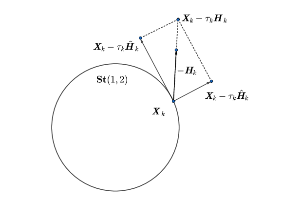
Figure 2. A new illustration of the update scheme (18) in Algorithm 1

Remark 4.7.

It was demonstrated in [82, Sec. 4.1] that the tangent vector $\boldsymbol{D}_{1/2}(\boldsymbol{X})\in\mathbf{T}_{\boldsymbol{X}}{\mathbf{St}(r,n)}$, as defined in (22), can be interpreted as the Riemannian gradient of $f(\boldsymbol{X})$ when considering a distinct Riemannian metric, namely the canonical metric. In Algorithm 1, if the scaling matrices $\boldsymbol{L}(\boldsymbol{X})$ and $\boldsymbol{R}(\boldsymbol{X})$ satisfy A and vary smoothly on $\mathcal{M}$, we can define a new Riemannian metric by

$$\langle\boldsymbol{V},\boldsymbol{V}^{\prime}\rangle_{\boldsymbol{X}}\stackrel{{\scriptstyle\sf def}}{{=}}\langle\boldsymbol{V},\boldsymbol{L}(\boldsymbol{X})^{-1}\boldsymbol{V}^{\prime}\boldsymbol{R}(\boldsymbol{X})^{-1}\rangle\text{ for all }\boldsymbol{V},\boldsymbol{V}^{\prime}\in\mathbf{T}_{\boldsymbol{X}}{\mathcal{M}}.$$

Then the Riemannian gradient under this new metric is $\boldsymbol{L}(\boldsymbol{X})\operatorname{grad}f(\boldsymbol{X})\boldsymbol{R}(\boldsymbol{X})$ by definition. In this scenario, according to Lemma 4.5, the tangent component $\tilde{\boldsymbol{H}}_{k}$ can also be interpreted as a Riemannian gradient of $f(\boldsymbol{X})$ at $\boldsymbol{X}_{k}$ under the above new Riemannian metric.

5. Properties of the projection onto a general compact manifold

In this section, we explore the geometric properties of the projection onto a general compact manifold, which will play a crucial role in the convergence analysis of our TGP algorithm framework in the next sections.

5.1. Uniqueness and smoothness of the projection

In the context of retraction-based line-search algorithms (2), a retraction is required to be smooth, at least in a local sense. In this subsection, we discuss the smoothness of the projection onto a general compact submanifold, as well as its uniqueness. We now begin with the following classical result, which demonstrates the well-defined nature of the projection onto a general compact manifold and derives its differential, indicating that this projection forms a retraction.

Lemma 5.1 ([4, Lem. 4]).

Let $\mathcal{M}^{\prime}\subseteq\mathbb{R}^{m}$ be a submanifold of class $C^{k}$ with $k\geq 2$ and $\mathcal{P}_{\mathcal{M}^{\prime}}$ be the projection onto $\mathcal{M}^{\prime}$. Given any $\bar{\boldsymbol{x}}\in\mathcal{M}^{\prime}$, there exists $\varrho_{\bar{\boldsymbol{x}}}>0$ such that $\mathcal{P}_{\mathcal{M}^{\prime}}(\boldsymbol{y})$ uniquely exists for all $\boldsymbol{y}\in\mathcal{B}(\bar{\boldsymbol{x}};\varrho_{\bar{\boldsymbol{x}}})$. Moreover, $\mathcal{P}_{\mathcal{M}^{\prime}}(\boldsymbol{y})$ is of class $C^{k-1}$ for $\boldsymbol{y}\in\mathcal{B}(\bar{\boldsymbol{x}};\varrho_{\bar{\boldsymbol{x}}})$, and $\mathrm{D}\mathcal{P}_{\mathcal{M}^{\prime}}(\bar{\boldsymbol{x}})=\mathcal{P}_{\mathbf{T}_{\bar{\boldsymbol{x}}}{\mathcal{M}}}$.

Based on the above Lemma 5.1, we now present a new result that reveals a stability property of the projection when the normal vector is relatively small. The proof of this result highly depends on that of [4, Lem. 4].

Lemma 5.2.

Let $\mathcal{M}^{\prime}\subseteq\mathbb{R}^{m}$ be a submanifold of class $C^{k}$ with $k\geq 2$ and $\mathcal{P}_{\mathcal{M}^{\prime}}$ be the projection onto $\mathcal{M}^{\prime}$. Let $\bar{\boldsymbol{x}}\in\mathcal{M}^{\prime}$ and $\varrho_{\bar{\boldsymbol{x}}}>0$ be as given in Lemma 5.1. Then, for all $\boldsymbol{x}\in\mathcal{M}^{\prime}\cap\mathcal{B}(\bar{\boldsymbol{x}};\varrho_{\bar{\boldsymbol{x}}})$ and $\boldsymbol{w}\in\mathbf{N}_{\boldsymbol{x}}{\mathcal{M}^{\prime}}$ satisfying $\boldsymbol{x}+\boldsymbol{w}\in\mathcal{B}(\bar{\boldsymbol{x}};\varrho_{\bar{\boldsymbol{x}}})$, we have $\mathcal{P}_{\mathcal{M}^{\prime}}(\boldsymbol{x}+\boldsymbol{w})=\boldsymbol{x}$.

Proof.

Consider the mapping $F:\mathbf{N}{\mathcal{M}^{\prime}}\to\mathbb{R}^{m},(\boldsymbol{x},\boldsymbol{w})\mapsto\boldsymbol{x}+\boldsymbol{w}$, where $\mathbf{N}{\mathcal{M}^{\prime}}\stackrel{{\scriptstyle\sf def}}{{=}}\{(\boldsymbol{x},\boldsymbol{w})\in\mathbb{R}^{m}\times\mathbb{R}^{m}:\boldsymbol{x}\in\mathcal{M}^{\prime},\boldsymbol{w}\in\mathbf{N}_{\boldsymbol{x}}{\mathcal{M}^{\prime}}\}$ denotes the normal bundle of $\mathcal{M}^{\prime}$. It follows from the construction of $\varrho_{\bar{\boldsymbol{x}}}$ in the proof of [4, Lem. 4] that $F$ is injective in $\mathcal{I}\stackrel{{\scriptstyle\sf def}}{{=}}\{(\boldsymbol{x},\boldsymbol{w}):\boldsymbol{x}\in\mathcal{M}^{\prime}\cap\mathcal{B}(\bar{\boldsymbol{x}};2\varrho_{\bar{\boldsymbol{x}}}),\boldsymbol{w}\in\mathbf{N}_{\boldsymbol{x}}{\mathcal{M}^{\prime}},\|\boldsymbol{w}\|<3\varrho_{\bar{\boldsymbol{x}}}\}$. For all $\boldsymbol{x}\in\mathcal{M}^{\prime}\cap\mathcal{B}(\bar{\boldsymbol{x}};\varrho_{\bar{\boldsymbol{x}}})$ and $\boldsymbol{w}\in\mathbf{N}_{\boldsymbol{x}}{\mathcal{M}^{\prime}}$ satisfying $\boldsymbol{x}+\boldsymbol{w}\in\mathcal{B}(\bar{\boldsymbol{x}};\varrho_{\bar{\boldsymbol{x}}})$, we know from Lemma 5.1 that $\mathcal{P}_{\mathcal{M}^{\prime}}(\boldsymbol{x}+\boldsymbol{w})$ uniquely exists and is in $\mathcal{M}^{\prime}\cap\mathcal{B}(\bar{\boldsymbol{x}};2\varrho_{\bar{\boldsymbol{x}}})$. By the definition of projection, $\mathcal{P}_{\mathcal{M}^{\prime}}(\boldsymbol{x}+\boldsymbol{w})$ is the solution of the optimization problem $\min_{\boldsymbol{z}\in\mathcal{M}^{\prime}}\|\boldsymbol{x}+\boldsymbol{w}-\boldsymbol{z}\|^{2}$. Thus, $\mathcal{P}_{\mathcal{M}^{\prime}}(\boldsymbol{x}+\boldsymbol{w})$ satisfies the first-order necessary condition: $\boldsymbol{x}+\boldsymbol{w}-\mathcal{P}_{\mathcal{M}^{\prime}}(\boldsymbol{x}+\boldsymbol{w})\in\mathbf{N}_{\mathcal{P}_{\mathcal{M}^{\prime}}(\boldsymbol{x}+\boldsymbol{w})}{\mathcal{M}^{\prime}}$. Therefore, there exists $\boldsymbol{w}^{\prime}\in\mathbf{N}_{\mathcal{P}_{\mathcal{M}^{\prime}}(\boldsymbol{x}+\boldsymbol{w})}{\mathcal{M}^{\prime}}$ such that $\boldsymbol{x}+\boldsymbol{w}=\mathcal{P}_{\mathcal{M}^{\prime}}(\boldsymbol{x}+\boldsymbol{w})+\boldsymbol{w}^{\prime}$. It follows from $\boldsymbol{x},\boldsymbol{x}+\boldsymbol{w}\in\mathcal{B}(\bar{\boldsymbol{x}};\varrho_{\bar{\boldsymbol{x}}})$ that $\|\boldsymbol{w}\|<2\varrho_{\bar{\boldsymbol{x}}}$. Since $\mathcal{P}_{\mathcal{M}^{\prime}}(\boldsymbol{x}+\boldsymbol{w})\in\mathcal{B}(\bar{\boldsymbol{x}};2\varrho_{\bar{\boldsymbol{x}}})$ and $\boldsymbol{x}\in\mathcal{B}(\bar{\boldsymbol{x}};\varrho_{\bar{\boldsymbol{x}}})$, we have $\|\boldsymbol{w}^{\prime}\|<3\varrho_{\bar{\boldsymbol{x}}}$. Thus, $(\boldsymbol{x},\boldsymbol{w})$ and $(\mathcal{P}_{\mathcal{M}^{\prime}}(\boldsymbol{x}+\boldsymbol{w}),\boldsymbol{w}^{\prime})$ belong to the region $\mathcal{I}$. It follows from $F(\boldsymbol{x},\boldsymbol{w})=\boldsymbol{x}+\boldsymbol{w}=\mathcal{P}_{\mathcal{M}^{\prime}}(\boldsymbol{x}+\boldsymbol{w})+\boldsymbol{w}^{\prime}=F(\mathcal{P}_{\mathcal{M}^{\prime}}(\boldsymbol{x}+\boldsymbol{w}),\boldsymbol{w}^{\prime})$ that $\boldsymbol{x}=\mathcal{P}_{\mathcal{M}^{\prime}}(\boldsymbol{x}+\boldsymbol{w})$. The proof is complete. ∎

Note that the above Lemmas 5.1 and 5.2 are both local results, i.e., the radius $\varrho_{\bar{\boldsymbol{x}}}$ depends on $\bar{\boldsymbol{x}}$. In this paper, by the compactness of $\mathcal{M}^{\prime}$, we can achieve the following stronger result where the radius is independent of the specific choice of $\bar{\boldsymbol{x}}$, denoted by $\varrho$.

Lemma 5.3.

Let $\mathcal{M}^{\prime}\subseteq\mathbb{R}^{m}$ be a compact submanifold of class $C^{k}$ with $k\geq 2$. Then there exists a positive constant $\varrho>0$ such that, for all $\boldsymbol{y}\in\mathcal{B}(\mathcal{M}^{\prime};\varrho),\mathcal{P}_{\mathcal{M}^{\prime}}(\boldsymbol{y})$ uniquely exists and is of class $C^{k-1}$. Moreover, for all $\boldsymbol{x}\in\mathcal{M}^{\prime}$ and $\boldsymbol{w}\in\mathbf{N}_{\boldsymbol{x}}{\mathcal{M}^{\prime}}$ satisfying $\|\boldsymbol{w}\|<\varrho$, we have

$$\mathcal{P}_{\mathcal{M}^{\prime}}(\boldsymbol{x}+\boldsymbol{w})=\boldsymbol{x}.$$ (31)

Proof.

It follows from Lemma 5.1 that for all $\bar{\boldsymbol{x}}\in\mathcal{M}^{\prime}$, there exists $\varrho_{\bar{\boldsymbol{x}}}>0$ such that $\mathcal{P}_{\mathcal{M}^{\prime}}(\boldsymbol{y})$ is of class $C^{k-1}$, $\mathcal{P}_{\mathcal{M}^{\prime}}(\boldsymbol{y})$ is unique for $\boldsymbol{y}\in\mathcal{B}(\bar{\boldsymbol{x}};\varrho_{\bar{\boldsymbol{x}}})$ and $\mathcal{P}_{\mathcal{M}^{\prime}}(\boldsymbol{x}+\boldsymbol{w})=\boldsymbol{x}$ for $\boldsymbol{x}\in\mathcal{M}^{\prime}\cap\mathcal{B}(\bar{\boldsymbol{x}};\varrho_{\bar{\boldsymbol{x}}})$ and $\boldsymbol{w}\in\mathbf{N}_{\boldsymbol{x}}{\mathcal{M}^{\prime}}$ satisfying $\boldsymbol{x}+\boldsymbol{w}\in\mathcal{B}(\bar{\boldsymbol{x}};\varrho_{\bar{\boldsymbol{x}}})$. We now first prove that there exists $\varrho_{1}>0$ such that $\bar{\mathcal{B}}(\mathcal{M}^{\prime};\varrho_{1})\subseteq\cup_{\bar{\boldsymbol{x}}\in\mathcal{M}^{\prime}}\mathcal{B}(\bar{\boldsymbol{x}};\varrho_{\bar{\boldsymbol{x}}})$ by contradiction. If not, then for all $k\geq 1$, there exists $\boldsymbol{y}_{k}\in\bar{\mathcal{B}}(\mathcal{M}^{\prime};1/k)$, such that $\boldsymbol{y}_{k}\not\in\cup_{\bar{\boldsymbol{x}}\in\mathcal{M}^{\prime}}\mathcal{B}(\bar{\boldsymbol{x}};\varrho_{\bar{\boldsymbol{x}}})$. Since $\mathcal{M}^{\prime}$ is bounded, the sequence $\{\boldsymbol{y}_{k}\}_{k\geq 1}$ is contained in a compact set, and thus it has an accumulation point, namely, $\boldsymbol{y}_{*}$. Noting that $d(\boldsymbol{y}_{k},\mathcal{M}^{\prime})<\frac{1}{k}$, we have $d(\boldsymbol{y}_{*},\mathcal{M}^{\prime})=0$, which implies $\boldsymbol{y}_{*}\in\mathcal{M}^{\prime}$ due to the compactness of $\mathcal{M}^{\prime}$. On the other hand, since $\cup_{\bar{\boldsymbol{x}}\in\mathcal{M}^{\prime}}\mathcal{B}(\bar{\boldsymbol{x}};\varrho_{\bar{\boldsymbol{x}}})$ is an open set and $\boldsymbol{y}_{k}\not\in\cup_{\bar{\boldsymbol{x}}\in\mathcal{M}^{\prime}}\mathcal{B}(\bar{\boldsymbol{x}};\varrho_{\bar{\boldsymbol{x}}})$ for all $k\geq 1$, the accumulation point $\boldsymbol{y}_{*}\not\in\cup_{\bar{\boldsymbol{x}}\in\mathcal{M}^{\prime}}\mathcal{B}(\bar{\boldsymbol{x}};\varrho_{\bar{\boldsymbol{x}}})$, which contradicts the fact that $\boldsymbol{y}_{*}\in\mathcal{M}^{\prime}$ and $\mathcal{M}^{\prime}\subseteq\cup_{\bar{\boldsymbol{x}}\in\mathcal{M}^{\prime}}\mathcal{B}(\bar{\boldsymbol{x}};\varrho_{\bar{\boldsymbol{x}}})$. Therefore, there exists $\varrho_{1}>0$ such that $\bar{\mathcal{B}}(\mathcal{M}^{\prime};\varrho_{1})\subseteq\cup_{\bar{\boldsymbol{x}}\in\mathcal{M}^{\prime}}\mathcal{B}(\bar{\boldsymbol{x}};\varrho_{\bar{\boldsymbol{x}}})$.

Then, by the Lebesgue number lemma [56], there exists $\varrho_{2}>0$, such that for each subset of $\bar{\mathcal{B}}(\mathcal{M}^{\prime};\varrho_{1})$ having diameter less than $\varrho_{2}$, there exists an element of $\{\mathcal{B}(\bar{\boldsymbol{x}};\varrho_{\bar{\boldsymbol{x}}}):\bar{\boldsymbol{x}}\in\mathcal{M}^{\prime}\}$ containing it. Denote $\varrho\stackrel{{\scriptstyle\sf def}}{{=}}\min\{\varrho_{1},\varrho_{2}/2\}$. Then we have $\mathcal{B}(\mathcal{M}^{\prime};\varrho)\subseteq\mathcal{B}(\mathcal{M}^{\prime};\varrho_{1})\subseteq\cup_{\bar{\boldsymbol{x}}\in\mathcal{M}^{\prime}}\mathcal{B}(\bar{\boldsymbol{x}};\varrho_{\bar{\boldsymbol{x}}})$. It follows from the definition of $\varrho_{\bar{\boldsymbol{x}}}$ that $\mathcal{P}_{\mathcal{M}^{\prime}}(\boldsymbol{y})$ uniquely exists and is of class $C^{k-1}$ for $\boldsymbol{y}\in\mathcal{B}(\mathcal{M}^{\prime};\varrho)$. Moreover, for all $\boldsymbol{x}\in\mathcal{M}^{\prime}$ and $\boldsymbol{w}\in\mathbf{N}_{\boldsymbol{x}}{\mathcal{M}^{\prime}}$ with $\|\boldsymbol{w}\|<\varrho$, the diameter of $\mathcal{B}(\boldsymbol{x};\varrho)$ is $2\varrho$, which satisfies $2\varrho\leq\varrho_{2}$. By the definition of $\varrho_{2}$, there exists $\bar{\boldsymbol{x}}\in\mathcal{M}^{\prime}$ such that $\mathcal{B}(\boldsymbol{x};\varrho)\subseteq\mathcal{B}(\bar{\boldsymbol{x}};\varrho_{\bar{\boldsymbol{x}}})$. In particular, we have $\boldsymbol{x},\boldsymbol{x}+\boldsymbol{w}\in\mathcal{B}(\bar{\boldsymbol{x}};\varrho_{\bar{\boldsymbol{x}}})$ for $\boldsymbol{w}\in\mathbf{N}_{\boldsymbol{x}}{\mathcal{M}^{\prime}}$ satisfying $\|\boldsymbol{w}\|<\varrho$. By the property of $\varrho_{\bar{\boldsymbol{x}}}$ stated in Lemma 5.2, we have $\mathcal{P}_{\mathcal{M}^{\prime}}(\boldsymbol{x}+\boldsymbol{w})=\boldsymbol{x}$. The proof is complete. ∎

Remark 5.4.

A subset $\mathcal{S}\subseteq\mathbb{R}^{m}$ is said to be proximally smooth with radius $\vartheta>0$ if the distance function $d(\boldsymbol{y},\mathcal{S})$ is continuously differentiable for $\boldsymbol{y}\in\mathcal{B}(\mathcal{S};\vartheta)$ [23], which is equivalent to the uniqueness of $\mathcal{P}_{\mathcal{S}}(\boldsymbol{x})$ when $\mathcal{S}$ is weakly closed [23, Thm. 4.11]. It follows from Lemma 5.3 that any compact $C^{2}$ submanifold $\mathcal{M}^{\prime}$ is proximally smooth, which is already known in the literature [23]. In fact, Lemma 5.3 can further indicate the higher-order smoothness of the distance function $d(\boldsymbol{y},\mathcal{M}^{\prime})$ if $\mathcal{M}^{\prime}$ is smooth enough, which might be of independent interest.

In this paper, we denote by $\varrho_{*}$ the maximum value of the above positive constant $\varrho$ in Lemma 5.3. For the cases of $\mathbf{St}(r,n)$ and $\mathbf{Gr}(p,n)$, we now estimate $\varrho_{*}$. Before that, we first present two lemmas concerning the projection onto $\mathbf{St}(r,n)$.

Lemma 5.5 ([34, Cor. 7.3.5]).

Let $\boldsymbol{Y},\tilde{\boldsymbol{Y}}\in\mathbb{R}^{n\times r}$ be two matrices with $\sigma_{1}(\boldsymbol{Y})\geq\cdots\geq\sigma_{r}(\boldsymbol{Y})$ and $\sigma_{1}(\tilde{\boldsymbol{Y}})\geq\cdots\geq\sigma_{r}(\tilde{\boldsymbol{Y}})$ as the non-increasingly ordered singular values, respectively. Then
(i) $\left|\sigma_{i}(\boldsymbol{Y})-\sigma_{i}(\tilde{\boldsymbol{Y}})\right|\leq\|\boldsymbol{Y}-\tilde{\boldsymbol{Y}}\|_{\infty}$ for $1\leq i\leq r$;
(ii) $\sum_{i=1}^{r}\left(\sigma_{i}(\boldsymbol{Y})-\sigma_{i}(\tilde{\boldsymbol{Y}})\right)^{2}\leq\|\boldsymbol{Y}-\tilde{\boldsymbol{Y}}\|^{2}$.

Lemma 5.6 ([32, Thm. 9.4.1], [33, Thm. 8.1], [34, Thm. 7.3.1]).

Let $\boldsymbol{Y}\in\mathbb{R}^{n\times r}$ with $1\leq r\leq n$. There exist $\boldsymbol{X}\in\mathbf{St}(r,n)$ and a unique positive semi-definite matrix $\boldsymbol{P}\in\mathbb{R}^{r\times r}$ such that $\boldsymbol{Y}$ has the polar decomposition $\boldsymbol{Y}=\boldsymbol{X}\boldsymbol{P}$. We say that $\boldsymbol{X}$ is the orthogonal polar factor and $\boldsymbol{P}$ is the positive semi-definite polar factor. Moreover,
(i) for any $\boldsymbol{X}^{\prime}\in\mathbf{St}(r,n)$, we have [33, pp. 217]

$$\langle\boldsymbol{X},\boldsymbol{Y}\rangle\geq\langle\boldsymbol{X}^{\prime},\boldsymbol{Y}\rangle;$$

(ii) $\boldsymbol{X}$ is the best orthogonal approximation [33, Thm. 8.4] to $\boldsymbol{Y}$, that is, for any $\boldsymbol{X}^{\prime}\in\mathbf{St}(r,n)$, we have

$$\|\boldsymbol{Y}-\boldsymbol{X}\|\leq\|\boldsymbol{Y}-\boldsymbol{X}^{\prime}\|;$$

(iii) if $\mathop{\operator@font rank}(\boldsymbol{Y})=r$, then $\boldsymbol{P}$ is positive definite and $\boldsymbol{X}$ is unique [33, Thm. 8.1]. Moreover, we have $\boldsymbol{X}=\boldsymbol{Y}(\boldsymbol{Y}^{{\sf T}}\boldsymbol{Y})^{-1/2}$ in this case.

Example 5.7 (Calculation of $\varrho_{*}$ on $\mathbf{St}(r,n)$).

The positive constant $\varrho_{*}=1$ on $\mathbf{St}(r,n)$. We first demonstrate that $\varrho_{*}\geq 1$. For any $\boldsymbol{Y}\in\mathbb{R}^{n\times r}$ satisfying $d(\boldsymbol{Y},\mathbf{St}(r,n))<1$, let $\boldsymbol{X}\in\mathbf{St}(r,n)$ be a projection of $\boldsymbol{Y}$. Then $\|\boldsymbol{Y}-\boldsymbol{X}\|<1$. It follows that

$$\sigma_{\min}(\boldsymbol{Y})=\sigma_{\min}(\boldsymbol{X}+(\boldsymbol{Y}-\boldsymbol{X}))\geq\sigma_{\min}(\boldsymbol{X})-\sigma_{\max}(\boldsymbol{Y}-\boldsymbol{X})\geq 1-\|\boldsymbol{Y}-\boldsymbol{X}\|>0,$$

where the first inequality follows from Lemma 5.5. Therefore, $\boldsymbol{Y}$ is nonsingular, implying that $\mathcal{P}_{\mathbf{St}(r,n)}(\boldsymbol{Y})$ is unique and $\mathcal{P}_{\mathbf{St}(r,n)}(\boldsymbol{Y})=\boldsymbol{Y}(\boldsymbol{Y}^{{\sf T}}\boldsymbol{Y})^{-1/2}$ by Lemma 5.6. It follows from the explicit expression of $\mathcal{P}_{\mathbf{St}(r,n)}(\boldsymbol{Y})$ that it is of class $C^{\infty}$ for all $\boldsymbol{Y}\in\mathbb{R}^{n\times r}$ satisfying $d(\boldsymbol{Y},\mathbf{St}(r,n))<1$. For any $\boldsymbol{W}\in\mathbf{N}_{\boldsymbol{X}}{\mathbf{St}(r,n)}$, by the representation of normal space (8), there exists $\boldsymbol{S}\in\mathop{\operator@font\bf symm}\left(\mathbb{R}^{r\times r}\right)$ such that $\boldsymbol{W}=\boldsymbol{X}\boldsymbol{S}$. If $\|\boldsymbol{W}\|<1$, we have $\lambda_{\min}(\boldsymbol{S})>-1$. Thus $\boldsymbol{X}+\boldsymbol{W}=\boldsymbol{X}(\boldsymbol{I}_{r}+\boldsymbol{S})$ is the polar decomposition of $\boldsymbol{X}+\boldsymbol{W}$ and $\mathcal{P}_{\mathbf{St}(r,n)}(\boldsymbol{X}+\boldsymbol{W})=\boldsymbol{X}$.

On the other hand, we show that $\varrho_{*}\leq 1$. For any $\boldsymbol{X}\in\mathbf{St}(r,n)$, let $\boldsymbol{Y}=[\boldsymbol{X}_{1:r-1},\boldsymbol{0}_{n}]\in\mathbb{R}^{n\times r}$, where $\boldsymbol{X}_{1:r-1}$ denotes the first $r-1$ columns of $\boldsymbol{X}$. Then $d(\boldsymbol{Y},\mathbf{St}(r,n))=1$ and the projection of $\boldsymbol{Y}$ is of the form $[\boldsymbol{X}_{1:r-1},\boldsymbol{y}]$, where $\boldsymbol{y}$ is any unit vector orthogonal to $\boldsymbol{X}_{1:r-1}$. Therefore, the projection $\mathcal{P}_{\mathbf{St}(r,n)}(\boldsymbol{Y})$ is not unique.

In the following lemma, we derive the properties of the projection onto $\mathbf{Gr}(p,n)$ and demonstrate that the computation of $\mathcal{P}_{\mathbf{Gr}(p,n)}$ can be achieved through eigenvalue decomposition.

Lemma 5.8.

Let $\boldsymbol{Y}\in\mathbb{R}^{n\times n}$ and $\mathop{\operator@font sym}\left(\boldsymbol{Y}\right)=\boldsymbol{Q}\boldsymbol{\Lambda}\boldsymbol{Q}^{{\sf T}}$ be the eigenvalue decomposition, where $\boldsymbol{Q}\in\mathbf{O}_{n}$ and $\boldsymbol{\Lambda}=\mathop{\operator@font\bf Diag}\{\lambda_{1},\lambda_{2},\ldots,\lambda_{n}\}$ with $\lambda_{1}\geq\lambda_{2}\geq\ldots\geq\lambda_{n}$. Then we have that
(i) $\mathcal{P}_{\mathbf{Gr}(p,n)}(\boldsymbol{Y})=\mathcal{P}_{\mathbf{Gr}(p,n)}(\mathop{\operator@font sym}\left(\boldsymbol{Y}\right))=\mathcal{P}_{\mathbf{Gr}(p,n)}(\boldsymbol{Y}^{{\sf T}})$;
(ii) $d(\boldsymbol{Y},\mathbf{Gr}(p,n))\geq d(\mathop{\operator@font sym}\left(\boldsymbol{Y}\right),\mathbf{Gr}(p,n))$;
(iii) $\boldsymbol{Q}\mathop{\operator@font\bf Diag}\{\boldsymbol{I}_{p},\boldsymbol{0}\}\boldsymbol{Q}^{{\sf T}}$ is a projection of $\boldsymbol{Y}$. This projection is unique if and only if $\lambda_{p}>\lambda_{p+1}$.

Proof.

(i) For any matrix $\boldsymbol{Y}\in\mathbb{R}^{n\times n}$ and $\boldsymbol{X}\in\mathbf{Gr}(p,n)$, we have $\|\boldsymbol{Y}-\boldsymbol{X}\|^{2}=\|\boldsymbol{Y}\|^{2}+\|\boldsymbol{X}\|^{2}-2\langle\boldsymbol{Y},\boldsymbol{X}\rangle=\|\boldsymbol{Y}\|^{2}+p-2\langle\boldsymbol{Y},\boldsymbol{X}\rangle$, where we use the fact that $\|\boldsymbol{X}\|^{2}=p$ for all $\boldsymbol{X}\in\mathbf{Gr}(p,n)$. Thus, $\mathcal{P}_{\mathbf{Gr}(p,n)}(\boldsymbol{Y})=\operatorname*{\arg\!\max}_{\boldsymbol{X}\in\mathbf{Gr}(p,n)}\langle\boldsymbol{Y},\boldsymbol{X}\rangle$. Note that $\boldsymbol{X}\in\mathbf{Gr}(p,n)$ is symmetric. We have $\langle\boldsymbol{Y},\boldsymbol{X}\rangle=\langle\boldsymbol{Y}^{{\sf T}},\boldsymbol{X}\rangle=\langle\mathop{\operator@font sym}\left(\boldsymbol{Y}\right),\boldsymbol{X}\rangle$. It follows that $\mathcal{P}_{\mathbf{Gr}(p,n)}(\boldsymbol{Y})=\operatorname*{\arg\!\max}_{\boldsymbol{X}\in\mathbf{Gr}(p,n)}\langle\boldsymbol{Y},\boldsymbol{X}\rangle=\operatorname*{\arg\!\max}_{\boldsymbol{X}\in\mathbf{Gr}(p,n)}\langle\boldsymbol{Y}^{{\sf T}},\boldsymbol{X}\rangle=\mathcal{P}_{\mathbf{Gr}(p,n)}(\boldsymbol{Y}^{{\sf T}})$. Similarly, we also have $\mathcal{P}_{\mathbf{Gr}(p,n)}(\boldsymbol{Y})=\mathcal{P}_{\mathbf{Gr}(p,n)}(\mathop{\operator@font sym}\left(\boldsymbol{Y}\right))$.
(ii) Let $\boldsymbol{X}$ be an arbitrary projection of $\boldsymbol{Y}$. It follows from (i) that $\boldsymbol{X}$ is also the projection of $\mathop{\operator@font sym}\left(\boldsymbol{Y}\right)$. Then we have

$$d^{2}(\boldsymbol{Y},\mathbf{Gr}(p,n)) =\|\boldsymbol{Y}-\boldsymbol{X}\|^{2}=\|\boldsymbol{Y}\|^{2}-2\langle\boldsymbol{Y},\boldsymbol{X}\rangle+\|\boldsymbol{X}\|^{2}=\|\boldsymbol{Y}\|^{2}-2\langle\mathop{\operator@font sym}\left(\boldsymbol{Y}\right),\boldsymbol{X}\rangle+\|\boldsymbol{X}\|^{2}$$

$$\geq\|\mathop{\operator@font sym}\left(\boldsymbol{Y}\right)\|^{2}-2\langle\mathop{\operator@font sym}\left(\boldsymbol{Y}\right),\boldsymbol{X}\rangle+\|\boldsymbol{X}\|^{2}=d^{2}(\mathop{\operator@font sym}\left(\boldsymbol{Y}\right),\mathbf{Gr}(p,n)).$$

(iii) For any $\boldsymbol{X}\in\mathbf{Gr}(p,n)$, there exists $\boldsymbol{U}\in\mathbf{St}(p,n)$ such that $\boldsymbol{X}=\boldsymbol{U}\boldsymbol{U}^{{\sf T}}$. It follows from the proof of (i) that

$$\mathcal{P}_{\mathbf{Gr}(p,n)}(\boldsymbol{Y}) =\mathcal{P}_{\mathbf{Gr}(p,n)}(\mathop{\operator@font sym}\left(\boldsymbol{Y}\right))=\operatorname*{\arg\!\max}_{\boldsymbol{X}\in\mathbf{Gr}(p,n)}\langle\mathop{\operator@font sym}\left(\boldsymbol{Y}\right),\boldsymbol{X}\rangle$$

$$=\left\{\boldsymbol{U}\boldsymbol{U}^{{\sf T}}:\boldsymbol{U}\in\operatorname*{\arg\!\max}_{\boldsymbol{U}\in\mathbf{St}(p,n)}\langle\mathop{\operator@font sym}\left(\boldsymbol{Y}\right),\boldsymbol{U}\boldsymbol{U}^{{\sf T}}\rangle\right\}.$$

Note that $\operatorname*{\arg\!\max}_{\boldsymbol{U}\in\mathbf{St}(p,n)}\langle\mathop{\operator@font sym}\left(\boldsymbol{Y}\right),\boldsymbol{U}\boldsymbol{U}^{{\sf T}}\rangle=\operatorname*{\arg\!\max}_{\boldsymbol{U}\in\mathbf{St}(p,n)}\langle\mathop{\operator@font sym}\left(\boldsymbol{Y}\right)\boldsymbol{U},\boldsymbol{U}\rangle$ is exactly the set of the eigenvectors of $\mathop{\operator@font sym}\left(\boldsymbol{Y}\right)$ corresponding to the top $p$ eigenvalues. It follows that $\boldsymbol{Q}^{{\sf T}}\mathop{\operator@font\bf Diag}\{\boldsymbol{I}_{p},\boldsymbol{0}\}\boldsymbol{Q}$ is a projection of $\boldsymbol{Y}$. Then, the proof is complete by using the fact that the solution of the top $p$ eigenvalue problem is unique (up to permutation) if and only if $\lambda_{p}>\lambda_{p+1}$. ∎

Example 5.9 (Calculation of $\varrho_{*}$ on $\mathbf{Gr}(p,n)$).

Note that $\mathbf{Gr}(n,n)=\{\boldsymbol{I}_{n}\}$ and $\mathbf{Gr}(0,n)=\{\boldsymbol{0}_{n\times n}\}$, and the projection always results in a single point in these two trivial cases. We assume that $1\leq p\leq n-1$. We show that $\varrho_{*}\leq 1/\sqrt{2}$. For any $\boldsymbol{X}\in\mathbf{Gr}(p,n)$, there exists $\boldsymbol{Q}\in\mathbf{O}_{n}$ such that $\boldsymbol{X}=\boldsymbol{Q}\mathop{\operator@font\bf Diag}\{\boldsymbol{I}_{p},\boldsymbol{0}\}\boldsymbol{Q}^{{\sf T}}$ by definition. Let $\boldsymbol{Y}=\boldsymbol{Q}\mathop{\operator@font\bf Diag}\{\boldsymbol{I}_{p-1},1/2,1/2,\boldsymbol{0}\}\boldsymbol{Q}^{{\sf T}}$. Then $\|\boldsymbol{X}-\boldsymbol{Y}\|=1/\sqrt{2}$ and, according to Lemma 5.8 (iii), the projection of $\boldsymbol{Y}$ is not unique, since its $p$th eigenvalue is equal to the $(p+1)$th one.

5.2. Geometric inequalities of the projection

Based on Lemma 5.3, we now derive the following relationship among the tangent component, normal component and the trajectory of iterates, which will play a crucial role in the convergence rate analysis of Algorithm 1.

Lemma 5.10.

Let $\mathcal{M}^{\prime}\subseteq\mathbb{R}^{m}$ be a compact submanifold of class $C^{3}$ and $\varrho_{*}>0$ be the positive constant defined after Lemma 5.3. Then for any $\delta\in(0,\varrho_{*}]$, there exist positive constants $L^{(\delta)}_{0},L^{(\delta)}_{1},L^{(\delta)}_{2}>0$ such that for all $\boldsymbol{x}\in\mathcal{M}^{\prime}$, $\boldsymbol{v}\in\mathbf{T}_{\boldsymbol{x}}{\mathcal{M}^{\prime}}$ and $\boldsymbol{w}\in\mathbf{N}_{\boldsymbol{x}}{\mathcal{M}^{\prime}}$ satisfying $\|\boldsymbol{w}\|\leq\varrho_{*}-\delta$, we have

$$\|\mathcal{P}_{\mathcal{M}^{\prime}}(\boldsymbol{x}+\boldsymbol{v}+\boldsymbol{w})-\boldsymbol{x}\| \leq L^{(\delta)}_{0}\|\boldsymbol{v}\|,$$ (32)

$$\|\mathcal{P}_{\mathcal{M}^{\prime}}(\boldsymbol{x}+\boldsymbol{v}+\boldsymbol{w})-\boldsymbol{x}-\boldsymbol{v}\| \leq L^{(\delta)}_{1}\|\boldsymbol{v}\|^{2}+L^{(\delta)}_{2}\|\boldsymbol{v}\|\|\boldsymbol{w}\|.$$ (33)

Proof.

Denote $\mathcal{U}\stackrel{{\scriptstyle\sf def}}{{=}}\bar{\mathcal{B}}(\mathcal{M}^{\prime};\varrho_{*}-\delta/2)$ for simplicity. By Lemma 5.3, the projection mapping $\mathcal{P}_{\mathcal{M}^{\prime}}$ is of class $C^{2}$ on $\mathcal{B}(\mathcal{M}^{\prime};\varrho^{*})$, and $\mathcal{P}_{\mathcal{M}^{\prime}}(\boldsymbol{x}+\boldsymbol{w})=\boldsymbol{x}$ for $\boldsymbol{w}\in\mathbf{N}_{\boldsymbol{x}}{\mathcal{M}^{\prime}}$ satisfying $\|\boldsymbol{w}\|\leq\varrho_{*}-\delta/2$. Since $\mathcal{U}\subseteq\mathcal{B}(\mathcal{M}^{\prime};\varrho^{*})$ is a compact set, both $\mathcal{P}_{\mathcal{M}^{\prime}}$ and its differential $\mathrm{D}\mathcal{P}_{\mathcal{M}^{\prime}}$ are Lipschitz continuous on $\mathcal{B}$. Denote the Lipschitz constants of them by $L_{\mathcal{P}_{\mathcal{M}^{\prime}}}$ and $L_{\mathrm{D}\mathcal{P}_{\mathcal{M}^{\prime}}}$, respectively. For any given $\boldsymbol{x}\in\mathcal{M}^{\prime}$, $\boldsymbol{v}\in\mathbf{T}_{\boldsymbol{x}}{\mathcal{M}^{\prime}}$ and $\boldsymbol{w}\in\mathbf{N}_{\boldsymbol{x}}{\mathcal{M}^{\prime}}$ satisfying $\|\boldsymbol{w}\|\leq\varrho_{*}-\delta$, we consider the following two cases.

Case I: $\|\boldsymbol{v}\|\leq\delta/2$. In this case, both $\boldsymbol{x}+\boldsymbol{w}$ and $\boldsymbol{x}+\boldsymbol{v}+\boldsymbol{w}$ are in $\mathcal{U}$ since $\|\boldsymbol{v}+\boldsymbol{w}\|\leq\|\boldsymbol{v}\|+\|\boldsymbol{w}\|\leq\varrho_{*}-\delta/2$. It follows from (31) and the Lipschitz continuity of $\mathcal{P}_{\mathcal{M}^{\prime}}$ on $\mathcal{U}$ that

$$\|\mathcal{P}_{\mathcal{M}^{\prime}}(\boldsymbol{x}+\boldsymbol{v}+\boldsymbol{w})-\boldsymbol{x}\|=\|\mathcal{P}_{\mathcal{M}^{\prime}}(\boldsymbol{x}+\boldsymbol{v}+\boldsymbol{w})-\mathcal{P}_{\mathcal{M}^{\prime}}(\boldsymbol{x}+\boldsymbol{w})\|\leq L_{\mathcal{P}_{\mathcal{M}^{\prime}}}\|\boldsymbol{v}\|.$$ (34)

Moreover, by using (31) and applying the descent lemma to the mapping $\mathcal{P}$ at $\boldsymbol{x}+\boldsymbol{w}$, we have

$$\|\mathcal{P}_{\mathcal{M}^{\prime}}(\boldsymbol{x}+\boldsymbol{v}+\boldsymbol{w})-\boldsymbol{x}-\mathrm{D}\mathcal{P}_{\mathcal{M}^{\prime}}(\boldsymbol{x}+\boldsymbol{w})[\boldsymbol{v}]\|$$

$$=\|\mathcal{P}_{\mathcal{M}^{\prime}}(\boldsymbol{x}+\boldsymbol{v}+\boldsymbol{w})-\mathcal{P}_{\mathcal{M}^{\prime}}(\boldsymbol{x}+\boldsymbol{w})-\mathrm{D}\mathcal{P}_{\mathcal{M}^{\prime}}(\boldsymbol{x}+\boldsymbol{w})[\boldsymbol{v}]\|\leq\frac{L_{\mathrm{D}\mathcal{P}_{\mathcal{M}^{\prime}}}}{2}\|\boldsymbol{v}\|^{2}.$$ (35)

Combining $\boldsymbol{v}=\mathcal{P}_{\mathbf{T}_{\boldsymbol{x}}{\mathcal{M}^{\prime}}}(\boldsymbol{v})=\mathrm{D}\mathcal{P}_{\mathcal{M}^{\prime}}(\boldsymbol{x})[\boldsymbol{v}]$ from Lemma 5.1 and the Lipschitz continuity of $\mathrm{D}\mathcal{P}_{\mathcal{M}^{\prime}}$, we obtain that

$$\|\mathrm{D}\mathcal{P}_{\mathcal{M}^{\prime}}(\boldsymbol{x}+\boldsymbol{w})[\boldsymbol{v}]-\boldsymbol{v}\| =\|\mathrm{D}\mathcal{P}_{\mathcal{M}^{\prime}}(\boldsymbol{x}+\boldsymbol{w})[\boldsymbol{v}]-\mathrm{D}\mathcal{P}_{\mathcal{M}^{\prime}}(\boldsymbol{x})[\boldsymbol{v}]\|$$

$$=\|(\mathrm{D}\mathcal{P}_{\mathcal{M}^{\prime}}(\boldsymbol{x}+\boldsymbol{w})-\mathrm{D}\mathcal{P}_{\mathcal{M}^{\prime}}(\boldsymbol{x}))[\boldsymbol{v}]\|\leq L_{\mathrm{D}\mathcal{P}_{\mathcal{M}^{\prime}}}\|\boldsymbol{v}\|\|\boldsymbol{w}\|.$$ (36)

It follows from (35) and (36) that

$$\|\mathcal{P}_{\mathcal{M}^{\prime}}(\boldsymbol{x}+\boldsymbol{v}+\boldsymbol{w})-\boldsymbol{x}-\boldsymbol{v}\|\leq\frac{L_{\mathrm{D}\mathcal{P}_{\mathcal{M}^{\prime}}}}{2}\|\boldsymbol{v}\|^{2}+L_{\mathrm{D}\mathcal{P}_{\mathcal{M}^{\prime}}}\|\boldsymbol{v}\|\|\boldsymbol{w}\|.$$ (37)

Case II: $\|\boldsymbol{v}\|>\delta/2$. Let $d_{\mathcal{M}^{\prime}}$ be the diameter of $\mathcal{M}^{\prime}$, i.e., $d_{\mathcal{M}^{\prime}}\stackrel{{\scriptstyle\sf def}}{{=}}\max\{\|\boldsymbol{x}-\boldsymbol{x}^{\prime}\|:\boldsymbol{x},\boldsymbol{x}^{\prime}\in\mathcal{M}^{\prime}\}$. Note that $\mathcal{P}_{\mathcal{M}^{\prime}}(\boldsymbol{x}+\boldsymbol{v}+\boldsymbol{w}),\boldsymbol{x}\in\mathcal{M}^{\prime}$ and $\|\boldsymbol{v}\|>\delta/2$. We have

$$\|\mathcal{P}_{\mathcal{M}^{\prime}}(\boldsymbol{x}+\boldsymbol{v}+\boldsymbol{w})-\boldsymbol{x}\| \leq d_{\mathcal{M}^{\prime}}\leq\frac{2d_{\mathcal{M}^{\prime}}}{\delta}\|\boldsymbol{v}\|,$$ (38)

$$\|\mathcal{P}_{\mathcal{M}^{\prime}}(\boldsymbol{x}+\boldsymbol{v}+\boldsymbol{w})-\boldsymbol{x}-\boldsymbol{v}\| \leq\|\mathcal{P}_{\mathcal{M}^{\prime}}(\boldsymbol{x}+\boldsymbol{v}+\boldsymbol{w})-\boldsymbol{x}\|+\|\boldsymbol{v}\|\leq\left(\frac{4d_{\mathcal{M}^{\prime}}}{\delta^{2}}+\frac{2}{\delta}\right)\|\boldsymbol{v}\|^{2}.$$ (39)

It follows from (34), (37), (38) and (39) that, if we set $L^{(\delta)}_{0}=\max\left\{L_{\mathcal{P}_{\mathcal{M}^{\prime}}},\frac{2d_{\mathcal{M}^{\prime}}}{\delta}\right\}$, $L^{(\delta)}_{1}=\max\left\{\frac{L_{\mathrm{D}\mathcal{P}_{\mathcal{M}^{\prime}}}}{2},\frac{4d_{\mathcal{M}^{\prime}}}{\delta^{2}}+\frac{2}{\delta}\right\}$ and $L^{(\delta)}_{2}=L_{\mathrm{D}\mathcal{P}_{\mathcal{M}^{\prime}}}$, the proof is complete. ∎

Remark 5.11.

In Lemma 5.3, we proved that, for all $\boldsymbol{y}$ satisfying $d(\boldsymbol{y},\mathcal{M}^{\prime})<\varrho_{*}$, the projection $\mathcal{P}_{\mathcal{M}^{\prime}}(\boldsymbol{y})$ uniquely exists. It’s worth noting that, in Lemma 5.10, the vector $\boldsymbol{x}+\boldsymbol{v}+\boldsymbol{w}$ may not satisfy this condition, and thus its projection is not necessarily unique. For example, when $\|\boldsymbol{v}\|>\delta/2$, it is possible that $d(\boldsymbol{x}+\boldsymbol{v}+\boldsymbol{w},\mathcal{M}^{\prime})\geq\varrho_{*}$. However, even in this case, the inequalities (32) and (33) still hold, considering $\mathcal{P}_{\mathcal{M}^{\prime}}(\boldsymbol{x}+\boldsymbol{v}+\boldsymbol{w})$ as any one projection of it.

Remark 5.12.

Let $\mathcal{M}^{\prime}\subseteq\mathbb{R}^{m}$ be a compact submanifold of class $C^{3}$ and $\operatorname{R}$ be a retraction on it. It was shown in [19, Eq. (B.3), (B.4)] that there exist positive constants $L_{0}^{\prime},L_{1}^{\prime}>0$, such that for all $\boldsymbol{x}\in\mathcal{M}^{\prime}$ and $\boldsymbol{v}\in\mathbf{T}_{\boldsymbol{x}}{\mathcal{M}^{\prime}}$,

$$\|\operatorname{R}_{\boldsymbol{x}}(\boldsymbol{v})-\boldsymbol{x}\|\leq L_{0}^{\prime}\|\boldsymbol{v}\|,\ \|\operatorname{R}_{\boldsymbol{x}}(\boldsymbol{v})-\boldsymbol{x}-\boldsymbol{v}\|\leq L_{1}^{\prime}\|\boldsymbol{v}\|^{2},$$ (40)

where the second inequality is referred to as second-order boundedness. In [52], a value of $L_{1}^{\prime}$ satisfying (40) is obtained for multiple kinds of retractions on $\mathbf{St}(r,n)$. Note that, if we set $\delta=\varrho_{*}$ in Lemma 5.10, then $\boldsymbol{w}=\boldsymbol{0}$ and the inequalities (32) and (33) reduce to

$$\|\mathcal{P}_{\mathcal{M}^{\prime}}(\boldsymbol{x}+\boldsymbol{v})-\boldsymbol{x}\|\leq L_{0}^{(\varrho_{*})}\|\boldsymbol{v}\|,\ \|\mathcal{P}_{\mathcal{M}^{\prime}}(\boldsymbol{x}+\boldsymbol{v})-\boldsymbol{x}-\boldsymbol{v}\|\leq L_{1}^{(\varrho_{*})}\|\boldsymbol{v}\|^{2},$$

for all $\boldsymbol{x}\in\mathcal{M}^{\prime}$ and $\boldsymbol{v}\in\mathbf{T}_{\boldsymbol{x}}{\mathcal{M}^{\prime}}$. Hence, constructing a retraction by the projection, Lemma 5.10 can be regarded as an extension of (40) allowing the appearance of a normal vector $\boldsymbol{w}\in\mathbf{N}_{\boldsymbol{x}}{\mathcal{M}^{\prime}}$.

Remark 5.13.

We would like to emphasize that it is not possible to improve Lemma 5.10 in the following two parts through the examination of specific examples within $\mathbf{St}(r,n)$.
(i) The condition that $\|\boldsymbol{w}\|\leq\varrho_{*}-\delta$ can not be weaker. Note that $\varrho_{*}=1$ on $\mathbf{St}(r,n)$ by Example 5.7. We just need to show that the inequality (32) may fail when $\|\boldsymbol{w}\|=1$ on $\mathbf{St}(r,n)$. Let $\boldsymbol{x}=(1,0)^{{\sf T}}\in\mathbf{St}(1,2)$, $\boldsymbol{w}=(-1,0)^{{\sf T}}$ and $\boldsymbol{v}=(0,\epsilon)^{{\sf T}}$ for some $\epsilon>0$. Then

$$\|\mathcal{P}_{\mathbf{St}(1,2)}(\boldsymbol{x}+\boldsymbol{v}+\boldsymbol{w})-\boldsymbol{x}\|=\|\mathcal{P}_{\mathbf{St}(1,2)}((0,\epsilon)^{{\sf T}})-(1,0)^{{\sf T}}\|=\|(0,1)^{{\sf T}}-(1,0)^{{\sf T}}\|=\sqrt{2}.$$

It is clear that there does not exist a positive constant $L_{0}>0$ such that the inequality (32) always holds.
(ii) The last term $\|\boldsymbol{v}\|\|\boldsymbol{w}\|$ in the inequality (33) can not be removed unless $\delta=\varrho$. For any $\delta\in(0,1)$, let $\boldsymbol{x}=(1,0)^{{\sf T}}\in\mathbf{St}(1,2)$, $\boldsymbol{v}=(0,\epsilon)^{{\sf T}}$ and $\boldsymbol{w}=(\delta/2-1,0)^{{\sf T}}$ for some $\epsilon>0$. Then

$$\left\|\mathcal{P}_{\mathbf{St}(1,2)}(\boldsymbol{x}+\boldsymbol{v}+\boldsymbol{w})-\boldsymbol{x}-\boldsymbol{v}\right\| =\left\|\mathcal{P}_{\mathbf{St}(1,2)}((\delta/2,\epsilon)^{{\sf T}})-(1,0)^{{\sf T}}-(0,\epsilon)^{{\sf T}}\right\|$$

$$=\left\|\frac{1}{\sqrt{\delta^{2}/4+\epsilon^{2}}}(\delta/2,\epsilon)^{{\sf T}}-(1,0)^{{\sf T}}-(0,\epsilon)^{{\sf T}}\right\|$$

$$=\left\|\frac{1}{\sqrt{\delta}^{2}/4+\epsilon^{2}}(\delta/2-\sqrt{\delta^{2}/4+\epsilon^{2}},\epsilon(1-\sqrt{\delta^{2}/4+\epsilon^{2}}))^{{\sf T}}\right\|$$

$$\geq\frac{\epsilon(1-\sqrt{\delta^{2}/4+\epsilon^{2}})}{\sqrt{\delta^{2}/4+\epsilon^{2}}}.$$

Since $\|\boldsymbol{v}\|=\epsilon$, we have that $\liminf_{\epsilon\to 0}\|\mathcal{P}_{\mathbf{St}(1,2)}(\boldsymbol{x}+\boldsymbol{v}+\boldsymbol{w})-\boldsymbol{x}-\boldsymbol{v}\|/\|\boldsymbol{v}\|\geq\delta/2-1$, implying that $\|\mathcal{P}_{\mathbf{St}(1,2)}(\boldsymbol{x}+\boldsymbol{v}+\boldsymbol{w})-\boldsymbol{x}-\boldsymbol{v}\|/\|\boldsymbol{v}\|^{2}\to\infty$ as $\epsilon\to 0$. Therefore, there does not exist $L_{1}>0$ such that $\|\mathcal{P}_{\mathbf{St}(1,2)}(\boldsymbol{x}+\boldsymbol{v}+\boldsymbol{w})-\boldsymbol{x}-\boldsymbol{v}\|\leq L_{1}\|\boldsymbol{v}\|^{2}$ for all $\boldsymbol{v}\in\mathbf{T}_{\boldsymbol{x}}{\mathcal{M}^{\prime}}$.

As two examples, we now go back to $\mathbf{St}(r,n)$ and $\mathbf{Gr}(p,n)$, and estimate $L_{0}$ based on the following lemmas.

Lemma 5.14 ([49, Thm. 1, Thm. 2]).

Let $\boldsymbol{Y},\bar{\boldsymbol{Y}}\in\mathbb{R}^{n\times r}$ be two matrices of full column rank, having the polar decompositions $\boldsymbol{Y}=\boldsymbol{X}\boldsymbol{P}$ and $\bar{\boldsymbol{Y}}=\bar{\boldsymbol{X}}\bar{\boldsymbol{P}}$, respectively. Then we have

$$\|\boldsymbol{X}-\bar{\boldsymbol{X}}\|\leq\left(\frac{2}{\sigma_{\rm min}(\boldsymbol{Y})+\sigma_{\rm min}(\bar{\boldsymbol{Y}})}+\frac{1}{\max(\sigma_{\rm min}(\boldsymbol{Y}),\sigma_{\rm min}(\bar{\boldsymbol{Y}}))}\right)\|\boldsymbol{Y}-\bar{\boldsymbol{Y}}\|.$$ (41)

Lemma 5.15.

Let $\boldsymbol{X}\in\mathbf{St}(r,n)$ and $\boldsymbol{S}\in\mathop{\operator@font\bf symm}\left(\mathbb{R}^{r\times r}\right)$. If $\lambda_{\min}(\boldsymbol{S})\geq\delta-1$ for some $\delta>0$, then for all $\boldsymbol{V}\in\mathbf{T}_{\boldsymbol{X}}{\mathbf{St}(r,n)}$, we have $\sigma_{\min}(\boldsymbol{X}+\boldsymbol{V}+\boldsymbol{X}\boldsymbol{S})\geq\delta$.

Proof.

Denote $\boldsymbol{S}_{\delta}\stackrel{{\scriptstyle\sf def}}{{=}}(1-\delta)\boldsymbol{I}_{r}+\boldsymbol{S}$. It is clear that $\boldsymbol{S}_{\delta}\succeq\boldsymbol{0}$. By equation (7), there exist $\boldsymbol{A}_{\boldsymbol{V}}\in\mathop{\operator@font\bf skew}\left(\mathbb{R}^{r\times r}\right)$ and $\boldsymbol{B}_{\boldsymbol{V}}\in\mathbb{R}^{(n-r)\times r}$ such that $\boldsymbol{V}=\boldsymbol{X}\boldsymbol{A}_{\boldsymbol{V}}+\boldsymbol{X}_{\perp}\boldsymbol{B}_{\boldsymbol{V}}$. Then we have

$$(\boldsymbol{X}+\boldsymbol{V}+\boldsymbol{X}\boldsymbol{S})^{{\sf T}}(\boldsymbol{X}+\boldsymbol{V}+\boldsymbol{X}\boldsymbol{S}) =(\boldsymbol{X}+\boldsymbol{X}\boldsymbol{A}_{\boldsymbol{V}}+\boldsymbol{X}_{\perp}\boldsymbol{B}_{\boldsymbol{V}}+\boldsymbol{X}\boldsymbol{S})^{{\sf T}}(\boldsymbol{X}+\boldsymbol{X}\boldsymbol{A}_{\boldsymbol{V}}+\boldsymbol{X}_{\perp}\boldsymbol{B}_{\boldsymbol{V}}+\boldsymbol{X}\boldsymbol{S})$$

$$=(\boldsymbol{X}(\boldsymbol{I}+\boldsymbol{S}+\boldsymbol{A}_{\boldsymbol{V}})+\boldsymbol{X}_{\perp}\boldsymbol{B}_{\boldsymbol{V}})^{{\sf T}}(\boldsymbol{X}(\boldsymbol{I}+\boldsymbol{S}+\boldsymbol{A}_{\boldsymbol{V}})+\boldsymbol{X}_{\perp}\boldsymbol{B}_{\boldsymbol{V}})$$

$$\stackrel{{\scriptstyle(a)}}{{=}}(\boldsymbol{I}+\boldsymbol{S}+\boldsymbol{A}_{\boldsymbol{V}})^{{\sf T}}(\boldsymbol{I}+\boldsymbol{S}+\boldsymbol{A}_{\boldsymbol{V}})+\boldsymbol{B}_{\boldsymbol{V}}^{{\sf T}}\boldsymbol{X}_{\perp}^{{\sf T}}\boldsymbol{X}_{\perp}\boldsymbol{B}_{\boldsymbol{V}}$$

$$\succeq(\boldsymbol{I}+\boldsymbol{S}+\boldsymbol{A}_{\boldsymbol{V}})^{{\sf T}}(\boldsymbol{I}+\boldsymbol{S}+\boldsymbol{A}_{\boldsymbol{V}})=(\delta\boldsymbol{I}+(\boldsymbol{A}_{\boldsymbol{V}}+\boldsymbol{S}_{\delta}))^{{\sf T}}(\delta\boldsymbol{I}+(\boldsymbol{A}_{\boldsymbol{V}}+\boldsymbol{S}_{\delta}))$$

$$=\delta^{2}\boldsymbol{I}+\delta(\boldsymbol{A}_{\boldsymbol{V}}^{{\sf T}}+\boldsymbol{S}_{\delta}^{{\sf T}}+\boldsymbol{A}_{\boldsymbol{V}}+\boldsymbol{S}_{\delta})+(\boldsymbol{A}_{\boldsymbol{V}}+\boldsymbol{S}_{\delta})^{{\sf T}}(\boldsymbol{A}_{\boldsymbol{V}}+\boldsymbol{S}_{\delta})\stackrel{{\scriptstyle(b)}}{{\succeq}}\delta^{2}\boldsymbol{I},$$

where the equality $(a)$ follows from that $\boldsymbol{X}^{{\sf T}}\boldsymbol{X}_{\perp}=\boldsymbol{0}$, and the inequality $(b)$ follows from that $\boldsymbol{A}_{\boldsymbol{V}}^{{\sf T}}+\boldsymbol{A}_{\boldsymbol{V}}=\boldsymbol{0}$ and $\boldsymbol{S}_{\delta}^{{\sf T}}=\boldsymbol{S}_{\delta}\succeq\boldsymbol{0}$. Therefore, we have $\sigma_{\min}(\boldsymbol{X}+\boldsymbol{V}+\boldsymbol{X}\boldsymbol{S})\geq\delta$. The proof is complete. ∎

Example 5.16 ($L_{0}^{(\delta)}$ on $\mathbf{St}(r,n)$).

Let $\boldsymbol{X}\in\mathbf{St}(r,n)$, $\boldsymbol{V}\in\mathbf{T}_{\boldsymbol{X}}{\mathbf{St}(r,n)}$ and $\boldsymbol{W}\in\mathbf{N}_{\boldsymbol{X}}{\mathbf{St}(r,n)}$. It follows from equation (8) that there exists $\boldsymbol{S}\in\mathop{\operator@font\bf symm}\left(\mathbb{R}^{r\times r}\right)$ such that $\boldsymbol{W}=\boldsymbol{X}\boldsymbol{S}$. When $\lambda_{\min}(\boldsymbol{S})\geq\delta-1$ from some $\delta>0$, we have $\sigma_{\min}(\boldsymbol{X}+\boldsymbol{W}+\boldsymbol{V})\geq\delta$ by Lemma 5.15. Since $\boldsymbol{X}+\boldsymbol{W}=\boldsymbol{X}(\boldsymbol{I}_{r}+\boldsymbol{S})$, we have $\sigma_{\min}(\boldsymbol{X}+\boldsymbol{W})\geq\delta$ and $\mathcal{P}_{\mathbf{St}(r,n)}(\boldsymbol{X}+\boldsymbol{W})=\boldsymbol{X}$. It follows from Lemma 5.14 that

$$\|\mathcal{P}_{\mathbf{St}(r,n)}(\boldsymbol{X}+\boldsymbol{V}+\boldsymbol{W})-\boldsymbol{X}\|=\|\mathcal{P}_{\mathbf{St}(r,n)}(\boldsymbol{X}+\boldsymbol{V}+\boldsymbol{W})-\mathcal{P}_{\mathbf{St}(r,n)}(\boldsymbol{X}+\boldsymbol{W})\|\leq\frac{2}{\delta}\|\boldsymbol{V}\|.$$

In particular, for $\boldsymbol{W}=\boldsymbol{X}\boldsymbol{S}$ satisfying $\|\boldsymbol{W}\|\leq 1-\delta$, we have $\lambda_{\min}(\boldsymbol{S})\geq\delta-1$, implying that the above inequality holds. Thus, $2/\delta$ is a choice of $L_{0}^{(\delta)}$ in (32).

Example 5.17 ($L_{0}^{(\delta)}$ on $\mathbf{Gr}(p,n)$).

Note that $\mathbf{Gr}(p,n)$ is proximally smooth with radius $1/\sqrt{2}$ as shown in [8]. We see that $\mathcal{P}_{\mathbf{Gr}(p,n)}$ is Lipschitz continuous with constant $L_{\mathcal{P}_{\mathbf{Gr}(p,n)}}=\sqrt{2}/\delta$ on $\mathcal{B}(\mathbf{Gr}(p,n);\varrho_{*}-\delta/2)$ by the property of proximally smooth sets [23, Thm. 4.8]. It follows from the construction of $L_{0}^{(\delta)}$ in the proof of Lemma 5.10 that $\max\left\{\sqrt{2}/\delta,4\sqrt{p}/\delta\right\}=4\sqrt{p}/\delta$ is a choice of $L_{0}^{(\delta)}$, where we used the fact that the diameter of $\mathbf{Gr}(p,n)$ is less than $2\sqrt{p}$.

While Lemma 5.10 established an upper bound of the distance between $\mathcal{P}_{\mathcal{M}^{\prime}}(\boldsymbol{x}+\boldsymbol{v}+\boldsymbol{w})$ and $\boldsymbol{x}$ in terms of the tangent component $\boldsymbol{v}$, we now present an inequality that builds its lower bound.

Lemma 5.18.

Let $\mathcal{M}^{\prime}\subseteq\mathbb{R}^{m}$ be a compact submanifold of class $C^{2}$. Then there exists a positive constant $L_{3}>0$, such that for all $\boldsymbol{x}\in\mathcal{M}^{\prime},\boldsymbol{v}\in\mathbf{T}_{\boldsymbol{x}}{\mathcal{M}^{\prime}}$ and $\boldsymbol{w}\in\mathbf{N}_{\boldsymbol{x}}{\mathcal{M}^{\prime}}$, we have

$$\|\mathcal{P}_{\mathcal{M}^{\prime}}(\boldsymbol{x}+\boldsymbol{v}+\boldsymbol{w})-\boldsymbol{x}\|\geq\frac{\|\boldsymbol{v}\|}{1+L_{3}\|\boldsymbol{v}+\boldsymbol{w}\|}.$$ (42)

Proof.

For any $\bar{\boldsymbol{x}}\in\mathcal{M}^{\prime}$, there exist a positive constant $\nu_{\bar{\boldsymbol{x}}}>0$ and a $C^{2}$ local defining function $\Phi_{\bar{\boldsymbol{x}}}:\mathcal{B}(\bar{\boldsymbol{x}};\nu_{\bar{\boldsymbol{x}}})\to\mathbb{R}^{m-d}$ such that $\Phi_{\bar{\boldsymbol{x}}}(\boldsymbol{x})=\boldsymbol{0}$ and $\boldsymbol{J}_{\Phi_{\bar{\boldsymbol{x}}}}(\boldsymbol{x})$ is of full rank for all $\boldsymbol{x}\in\mathcal{M}^{\prime}\cap\mathcal{B}(\bar{\boldsymbol{x}};\nu_{\bar{\boldsymbol{x}}})$, where $d$ is the dimension of $\mathcal{M}^{\prime}$ and $\boldsymbol{J}_{\Phi_{\bar{\boldsymbol{x}}}}(\boldsymbol{x})\in\mathbb{R}^{(m-d)\times m}$ is the Jacobian matrix of $\Phi_{\bar{\boldsymbol{x}}}$ at $\boldsymbol{x}$. Note that $\mathbf{T}_{\boldsymbol{x}}{\mathcal{M}^{\prime}}=\operatorname{ker}(\mathrm{D}\Phi_{\bar{\boldsymbol{x}}}(\boldsymbol{x}))$ by [3, Eq. 3.19] and $\mathrm{D}\Phi_{\bar{\boldsymbol{x}}}(\boldsymbol{x})[\boldsymbol{u}]=\boldsymbol{J}_{\Phi_{\bar{\boldsymbol{x}}}}(\boldsymbol{x})\boldsymbol{u}$. It follows that, for all $\boldsymbol{x}\in\mathcal{M}^{\prime}\cap\mathcal{B}(\bar{\boldsymbol{x}};\nu_{\bar{\boldsymbol{x}}})$, we have

$$\mathcal{P}_{\mathbf{T}_{\boldsymbol{x}}{\mathcal{M}^{\prime}}}(\boldsymbol{u})=\left(\boldsymbol{I}_{m}-\boldsymbol{J}_{\Phi_{\bar{\boldsymbol{x}}}}(\boldsymbol{x})^{{\sf T}}(\boldsymbol{J}_{\Phi_{\bar{\boldsymbol{x}}}}(\boldsymbol{x})\boldsymbol{J}_{\Phi_{\bar{\boldsymbol{x}}}}(\boldsymbol{x})^{{\sf T}})^{-1}\boldsymbol{J}_{\Phi_{\bar{\boldsymbol{x}}}}(\boldsymbol{x})\right)\boldsymbol{u},\ \forall\boldsymbol{u}\in\mathbb{R}^{m}.$$ (43)

Since $\mathcal{M}^{\prime}\subseteq\cup_{\bar{\boldsymbol{x}}\in\mathcal{M}^{\prime}}\mathcal{B}(\bar{\boldsymbol{x}};\nu_{\bar{\boldsymbol{x}}}/2)$ and $\mathcal{M}^{\prime}$ is compact, there exists a finite subset $\mathcal{S}\subseteq\mathcal{M}^{\prime}$ such that $\mathcal{M}^{\prime}\subseteq\cup_{\bar{\boldsymbol{x}}\in\mathcal{S}}\mathcal{B}(\bar{\boldsymbol{x}};\nu_{\bar{\boldsymbol{x}}}/2)$. Since $\boldsymbol{I}_{m}-\boldsymbol{J}_{\Phi_{\bar{\boldsymbol{x}}}}(\boldsymbol{x})^{{\sf T}}(\boldsymbol{J}_{\Phi_{\bar{\boldsymbol{x}}}}(\boldsymbol{x})\boldsymbol{J}_{\Phi_{\bar{\boldsymbol{x}}}}(\boldsymbol{x})^{{\sf T}})^{-1}\boldsymbol{J}_{\Phi_{\bar{\boldsymbol{x}}}}(\boldsymbol{x})$ is continuously differentiable for all $\boldsymbol{x}\in\bar{\mathcal{B}}(\bar{\boldsymbol{x}};\nu_{\bar{\boldsymbol{x}}}/2)$, it is Lipschitz continuous on $\bar{\mathcal{B}}(\bar{\boldsymbol{x}};\nu_{\bar{\boldsymbol{x}}}/2)$. Let $L_{\mathcal{P}_{\mathbf{T}_{\bar{\boldsymbol{x}}}{\mathcal{M}^{\prime}}}}$ be its Lipschitz constant and $L_{\mathcal{P}_{\mathbf{T}{\mathcal{M}^{\prime}}}}\stackrel{{\scriptstyle\sf def}}{{=}}\max_{\bar{\boldsymbol{x}}\in\mathcal{S}}L_{\mathcal{P}_{\mathbf{T}_{\bar{\boldsymbol{x}}}{\mathcal{M}^{\prime}}}}$. By a similar argument as in the proof of Lemma 5.3 and using the Lebesgue number lemma, we know that there exists $\nu>0$ such that, for all $\boldsymbol{x},\boldsymbol{z}\in\mathcal{M}^{\prime}$ satisfying $\|\boldsymbol{x}-\boldsymbol{z}\|<\nu$, there exists $\bar{\boldsymbol{x}}\in\mathcal{S}$ such that $\boldsymbol{x},\boldsymbol{z}\in\mathcal{B}(\bar{\boldsymbol{x}};\nu_{\bar{\boldsymbol{x}}}/2)$. Then for such $\boldsymbol{x}$ and $\boldsymbol{z}$, using (43) and the definition of $L_{\mathcal{P}_{\mathbf{T}_{\bar{\boldsymbol{x}}}{\mathcal{M}^{\prime}}}}$, we have

$$\|\mathcal{P}_{\mathbf{T}_{\boldsymbol{x}}{\mathcal{M}^{\prime}}}(\boldsymbol{u})-\mathcal{P}_{\mathbf{T}_{\boldsymbol{z}}{\mathcal{M}^{\prime}}}(\boldsymbol{u})\|\leq L_{\mathcal{P}_{\mathbf{T}_{\bar{\boldsymbol{x}}}{\mathcal{M}^{\prime}}}}\|\boldsymbol{u}\|\leq L_{\mathcal{P}_{\mathbf{T}{\mathcal{M}^{\prime}}}}\|\boldsymbol{u}\|,\ \forall\boldsymbol{u}\in\mathbb{R}^{m}.$$ (44)

Denote $\boldsymbol{z}\stackrel{{\scriptstyle\sf def}}{{=}}\mathcal{P}_{\mathcal{M}^{\prime}}(\boldsymbol{x}+\boldsymbol{v}+\boldsymbol{w})$ and $\boldsymbol{w}^{\prime}\stackrel{{\scriptstyle\sf def}}{{=}}\boldsymbol{z}-(\boldsymbol{x}+\boldsymbol{v}+\boldsymbol{w})$ for simplicity. Since $\boldsymbol{z}$ is a projection of $\boldsymbol{x}+\boldsymbol{v}+\boldsymbol{w}$, we have $\boldsymbol{w}^{\prime}\in\mathbf{N}_{\boldsymbol{z}}{\mathcal{M}}$. We consider the following two cases.

Case I: $\|\boldsymbol{z}-\boldsymbol{x}\|<\nu$. By (44), we have that

$$\|\boldsymbol{z}-\boldsymbol{x}\| =\|\boldsymbol{v}+\boldsymbol{w}+\boldsymbol{w}^{\prime}\|\geq\|\mathcal{P}_{\mathbf{T}_{\boldsymbol{z}}{\mathcal{M}}}(\boldsymbol{v}+\boldsymbol{w}+\boldsymbol{w}^{\prime})\|=\|\mathcal{P}_{\mathbf{T}_{\boldsymbol{z}}{\mathcal{M}}}(\boldsymbol{v}+\boldsymbol{w})\|$$

$$\geq\|\mathcal{P}_{\mathbf{T}_{\boldsymbol{x}}{\mathcal{M}^{\prime}}}(\boldsymbol{v}+\boldsymbol{w})\|-\|\mathcal{P}_{\mathbf{T}_{\boldsymbol{z}}{\mathcal{M}}}(\boldsymbol{v}+\boldsymbol{w})-\mathcal{P}_{\mathbf{T}_{\boldsymbol{x}}{\mathcal{M}^{\prime}}}(\boldsymbol{v}+\boldsymbol{w})\|$$

$$\geq\|\boldsymbol{v}\|-L_{\mathcal{P}_{\mathbf{T}{\mathcal{M}^{\prime}}}}\|\boldsymbol{z}-\boldsymbol{x}\|\|\boldsymbol{v}+\boldsymbol{w}\|.$$

It follows that $\|\boldsymbol{z}-\boldsymbol{x}\|\geq\|\boldsymbol{v}\|/(1+L_{\mathcal{P}_{\mathbf{T}{\mathcal{M}^{\prime}}}}\|\boldsymbol{v}+\boldsymbol{w}\|).$

Case II: $\|\boldsymbol{z}-\boldsymbol{x}\|\geq\nu$. Noting that $\|\boldsymbol{v}+\boldsymbol{w}\|\geq\|\boldsymbol{v}\|$, we have

$$\|\boldsymbol{z}-\boldsymbol{x}\|\geq\nu\geq\nu\|\boldsymbol{v}\|/\|\boldsymbol{v}+\boldsymbol{w}\|\geq\|\boldsymbol{v}\|/(1+\|\boldsymbol{v}+\boldsymbol{w}\|/\nu).$$ (45)

Then, the proof is complete by setting $L_{3}=\max\{L_{\mathcal{P}_{\mathbf{T}{\mathcal{M}^{\prime}}}},1/\nu\}$. ∎

Within the context of the Stiefel manifold, we present the following proposition, which offers a more specific result.

Lemma 5.19.

For all $\boldsymbol{X}\in\mathbf{St}(r,n),\boldsymbol{V}\in\mathbf{T}_{\boldsymbol{X}}{\mathbf{St}(r,n)}$ and $\boldsymbol{W}\in\mathbf{N}_{\boldsymbol{X}}{\mathbf{St}(r,n)}$ satisfying $\|\boldsymbol{X}+\boldsymbol{V}+\boldsymbol{W}\|\neq 0$, we have that

$$\|\mathcal{P}_{\mathbf{St}(r,n)}(\boldsymbol{X}+\boldsymbol{V}+\boldsymbol{W})-\boldsymbol{X}\|\geq\frac{\|\boldsymbol{V}\|}{(r+1)\|\boldsymbol{X}+\boldsymbol{V}+\boldsymbol{W}\|}.$$

Proof.

Denote $\boldsymbol{Z}\stackrel{{\scriptstyle\sf def}}{{=}}\mathcal{P}_{\mathbf{St}(r,n)}(\boldsymbol{X}+\boldsymbol{V}+\boldsymbol{W})$ for simplicity. By Lemma 5.6, there exists a positive semi-definite matrix $\boldsymbol{P}\in\mathop{\operator@font\bf symm}\left(\mathbb{R}^{r\times r}\right)$ such that $\boldsymbol{X}+\boldsymbol{V}+\boldsymbol{W}=\boldsymbol{Z}\boldsymbol{P}$. Since $\boldsymbol{V}\in\mathbf{T}_{\boldsymbol{X}}{\mathbf{St}(r,n)}$, we have $\boldsymbol{X}^{{\sf T}}\boldsymbol{V}+\boldsymbol{V}^{{\sf T}}\boldsymbol{X}=\boldsymbol{0}$ by (6). For $\boldsymbol{W}\in\mathbf{N}_{\boldsymbol{X}}{\mathbf{St}(r,n)}$, there exists $\boldsymbol{S}\in\mathop{\operator@font\bf symm}\left(\mathbb{R}^{r\times r}\right)$ such that $\boldsymbol{W}=\boldsymbol{X}\boldsymbol{S}$ by (8), implying that $\boldsymbol{X}\boldsymbol{X}^{{\sf T}}\boldsymbol{W}=\boldsymbol{W}=\boldsymbol{X}\boldsymbol{W}^{{\sf T}}\boldsymbol{X}$. Then we have

$$\|\boldsymbol{V}\| =\frac{1}{2}\left\|\left(\boldsymbol{X}+\boldsymbol{V}+\boldsymbol{W}-\boldsymbol{X}\boldsymbol{X}^{{\sf T}}(\boldsymbol{X}+\boldsymbol{V}+\boldsymbol{W})\right)+\left(\boldsymbol{X}+\boldsymbol{V}+\boldsymbol{W}-\boldsymbol{X}(\boldsymbol{X}+\boldsymbol{V}+\boldsymbol{W})^{{\sf T}}\boldsymbol{X}\right)\right\|$$

$$=\frac{1}{2}\|(\boldsymbol{Z}\boldsymbol{P}-\boldsymbol{X}\boldsymbol{X}^{{\sf T}}\boldsymbol{Z}\boldsymbol{P})+(\boldsymbol{Z}\boldsymbol{P}-\boldsymbol{X}\boldsymbol{P}\boldsymbol{Z}^{{\sf T}}\boldsymbol{X})\|$$

$$=\frac{1}{2}\left\|\left((\boldsymbol{Z}-\boldsymbol{X})\boldsymbol{P}-\boldsymbol{X}\boldsymbol{X}^{{\sf T}}(\boldsymbol{Z}-\boldsymbol{X})\boldsymbol{P}\right)+\left((\boldsymbol{Z}-\boldsymbol{X})\boldsymbol{P}-\boldsymbol{X}\boldsymbol{P}(\boldsymbol{Z}-\boldsymbol{X})^{{\sf T}}\boldsymbol{X}\right)\right\|$$

$$\leq\frac{1}{2}\left(\|(\boldsymbol{Z}-\boldsymbol{X})\boldsymbol{P}\|+\|\boldsymbol{X}\boldsymbol{X}^{{\sf T}}\|\|(\boldsymbol{Z}-\boldsymbol{X})\boldsymbol{P}\|+\|(\boldsymbol{Z}-\boldsymbol{X})\boldsymbol{P}\|+\|\boldsymbol{X}\|\|\boldsymbol{P}(\boldsymbol{Z}-\boldsymbol{X})^{{\sf T}}\|\|\boldsymbol{X}\|\right)$$

$$\leq(r+1)\|\boldsymbol{Z}-\boldsymbol{X}\|\|\boldsymbol{X}+\boldsymbol{V}+\boldsymbol{W}\|,$$

where the last inequality follows from $\|\boldsymbol{P}\|=\|\boldsymbol{X}+\boldsymbol{V}+\boldsymbol{W}\|$ and $\|\boldsymbol{X}\|=\sqrt{r}$. The proof is complete. ∎

5.3. Decrease of function value after the projection

We end this section with an inequality similar to the descent lemma, which helps to estimate the decrease of function value in each iteration. Before that, let us first recall the following Riemannian subgradient inequality for weakly convex functions over compact manifolds.

Lemma 5.20 ([50, Cor. 1]).

Let $\mathcal{M}^{\prime}\subseteq\mathbb{R}^{m}$ be a compact submanifold given by $\mathcal{M}^{\prime}=\{\boldsymbol{x}\in\mathbb{R}^{m}:F(\boldsymbol{x})=\boldsymbol{0}\}$, where $F:\mathbb{R}^{m}\to\mathbb{R}^{m^{\prime}}$ is a smooth mapping whose derivative $\mathrm{D}F(\boldsymbol{x})$ at $\boldsymbol{x}$ has full row rank for all $\boldsymbol{x}\in\mathcal{M}^{\prime}$. Then, for any weakly convex function $g:\mathbb{R}^{m}\to\mathbb{R}$, there exists a positive constant $c>0$ such that

$$g(\boldsymbol{y})-g(\boldsymbol{x})-\left\langle\tilde{\nabla}_{R}g(\boldsymbol{x}),\boldsymbol{y}-\boldsymbol{x}\right\rangle\geq-c\|\boldsymbol{y}-\boldsymbol{x}\|^{2}$$ (46)

for all $\boldsymbol{x},\boldsymbol{y}\in\mathcal{M}^{\prime}$ and $\tilde{\nabla}_{R}g(\boldsymbol{x})\in\partial_{R}g(\boldsymbol{x})$, where $\partial_{R}g(\boldsymbol{x})$ denotes the projection of the subdifferential $\partial g(\boldsymbol{x})$ onto the tangent space $\mathbf{T}_{\boldsymbol{x}}{\mathcal{M}^{\prime}}$.

Remark 5.21.

(i) By checking the proof of [50, Cor. 1], it can be verified that the result remains valid for $g$ which is weakly convex on a bounded convex set containing $\mathcal{M}^{\prime}$. We now argue that the assumption on $\mathcal{M}^{\prime}$ can be replaced by that $\mathcal{M}^{\prime}$ is a compact submanifold of class $C^{2}$. In fact, by the original proof, it suffices to show that there exists a positive constant $a>0$ such that for all $\boldsymbol{x},\boldsymbol{y}\in\mathcal{M}^{\prime}$, $\|\mathcal{P}_{\mathbf{N}_{\boldsymbol{x}}{\mathcal{M}^{\prime}}}(\boldsymbol{x}-\boldsymbol{y})\|\leq a\|\boldsymbol{x}-\boldsymbol{y}\|^{2}$. We use $\nu$, $\nu_{\bar{\boldsymbol{x}}}$ and $\mathcal{S}$ defined in the proof of Lemma 5.18. When $\|\boldsymbol{x}-\boldsymbol{y}\|<\nu$, there exists $\bar{\boldsymbol{x}}\in\mathcal{M}^{\prime}$ such that $\boldsymbol{x},\boldsymbol{y}\in\mathcal{B}(\bar{\boldsymbol{x}};\nu_{\bar{\boldsymbol{x}}}/2)$. Let $L_{\mathrm{D}\Phi_{\bar{\boldsymbol{x}}}}$ be the Lipschitz constant of $\mathrm{D}\Phi_{\bar{\boldsymbol{x}}}$ on the compact set $\bar{\mathcal{B}}(\bar{\boldsymbol{x}};\nu_{\bar{\boldsymbol{x}}}/2)$ and $L_{\mathrm{D}\Phi}\stackrel{{\scriptstyle\sf def}}{{=}}\max_{\bar{\boldsymbol{x}}\in\mathcal{S}}L_{\mathrm{D}\Phi_{\bar{\boldsymbol{x}}}}$. It follows from the descent lemma that

$$\|\boldsymbol{J}_{\Phi_{\bar{\boldsymbol{x}}}}(\boldsymbol{y}-\boldsymbol{x})\|=\|\Phi_{\bar{\boldsymbol{x}}}(\boldsymbol{y})-\Phi_{\bar{\boldsymbol{x}}}(\boldsymbol{x})-\boldsymbol{J}_{\Phi_{\bar{\boldsymbol{x}}}}(\boldsymbol{y}-\boldsymbol{x})\|\leq\frac{L_{\mathrm{D}\Phi}}{2}\|\boldsymbol{y}-\boldsymbol{x}\|^{2},$$

where we used the fact that $\Phi_{\bar{\boldsymbol{x}}}(\boldsymbol{x})=\Phi_{\bar{\boldsymbol{x}}}(\boldsymbol{y})=\boldsymbol{0}$ for $\boldsymbol{x},\boldsymbol{y}\in\mathcal{M}^{\prime}\cap\bar{\mathcal{B}}(\bar{\boldsymbol{x}};\nu_{\bar{\boldsymbol{x}}}/2)$. Denote $\Delta_{\boldsymbol{J}_{\bar{\boldsymbol{x}}}}\stackrel{{\scriptstyle\sf def}}{{=}}\max_{\boldsymbol{x}\in\bar{\mathcal{B}}(\bar{\boldsymbol{x}};\nu_{\bar{\boldsymbol{x}}}/2)}\|\boldsymbol{J}_{\Phi_{\bar{\boldsymbol{x}}}}(\boldsymbol{x})^{{\sf T}}(\boldsymbol{J}_{\Phi_{\bar{\boldsymbol{x}}}}(\boldsymbol{x})\boldsymbol{J}_{\Phi_{\bar{\boldsymbol{x}}}}(\boldsymbol{x})^{{\sf T}})^{-1}\|$, $\Delta_{\boldsymbol{J}}\stackrel{{\scriptstyle\sf def}}{{=}}\max_{\bar{\boldsymbol{x}}\in\mathcal{S}}\Delta_{\boldsymbol{J}_{\bar{\boldsymbol{x}}}}$. Then, by (43), we have that

$$\|\mathcal{P}_{\mathbf{N}_{\boldsymbol{x}}{\mathcal{M}^{\prime}}}(\boldsymbol{x}-\boldsymbol{y})\|=\left\|\left(\boldsymbol{J}_{\Phi_{\bar{\boldsymbol{x}}}}(\boldsymbol{x})^{{\sf T}}(\boldsymbol{J}_{\Phi_{\bar{\boldsymbol{x}}}}(\boldsymbol{x})\boldsymbol{J}_{\Phi_{\bar{\boldsymbol{x}}}}(\boldsymbol{x})^{{\sf T}})^{-1}\right)\left(\boldsymbol{J}_{\Phi_{\bar{\boldsymbol{x}}}}(\boldsymbol{y}-\boldsymbol{x})\right)\right\|\leq\frac{\Delta_{\boldsymbol{J}}L_{\mathrm{D}\Phi}}{2}\|\boldsymbol{x}-\boldsymbol{y}\|^{2}.$$

In the other case where $\|\boldsymbol{x}-\boldsymbol{y}\|\geq\nu$, we have $\|\mathcal{P}_{\mathbf{N}_{\boldsymbol{x}}{\mathcal{M}^{\prime}}}(\boldsymbol{x}-\boldsymbol{y})\|\leq\|\boldsymbol{x}-\boldsymbol{y}\|\leq\frac{1}{\nu}\|\boldsymbol{x}-\boldsymbol{y}\|^{2}$. Thus, if we set $a\stackrel{{\scriptstyle\sf def}}{{=}}\max\left\{\frac{1}{\nu},\frac{\Delta_{\boldsymbol{J}}L_{\mathrm{D}\Phi}}{2}\right\}$, it satisfies $\|\mathcal{P}_{\mathbf{N}_{\boldsymbol{x}}{\mathcal{M}^{\prime}}}(\boldsymbol{x}-\boldsymbol{y})\|\leq a\|\boldsymbol{x}-\boldsymbol{y}\|^{2}$ for all $\boldsymbol{x},\boldsymbol{y}\in\mathcal{M}^{\prime}$.
(ii) If the function $g$ in Lemma 5.20 is continuously differentiable with a Lipschitz continuous gradient in a convex set containing $\mathcal{M}^{\prime}$, then we can prove the following inequality by a proof similar to that of Lemma 5.20:

$$\left|g(\boldsymbol{y})-g(\boldsymbol{x})-\left\langle\operatorname{grad}g(\boldsymbol{x}),\boldsymbol{y}-\boldsymbol{x}\right\rangle\right|\leq c\|\boldsymbol{y}-\boldsymbol{x}\|^{2}.$$ (47)

Based on Lemma 5.20 and our previous result Lemma 5.10, we are now able to prove the following result. It is worth noticing that the following lemma holds for all projections of $\boldsymbol{x}+\boldsymbol{v}+\boldsymbol{w}$ even if the projection is not unique.

Lemma 5.22.

Let $\mathcal{M}^{\prime}\subseteq\mathbb{R}^{m}$ be a compact submanifold of class $C^{3}$, $g:\mathbb{R}^{m}\to\mathbb{R}$ be a twice continuously differentiable function, and $\delta\in(0,\varrho_{*}]$ be a fixed constant, where $\varrho_{*}$ is the constant related to $\mathcal{M}^{\prime}$ defined after Lemma 5.3. Then there exist positive constants $\Gamma_{1}^{(\delta)},\Gamma_{2}^{(\delta)}>0$, such that for all $\boldsymbol{x}\in\mathcal{M}^{\prime}$, $\boldsymbol{v}\in\mathbf{T}_{\boldsymbol{x}}{\mathcal{M}^{\prime}}$ and $\boldsymbol{w}\in\mathbf{N}_{\boldsymbol{x}}{\mathcal{M}^{\prime}}$ satisfying $\|\boldsymbol{w}\|\leq\varrho_{*}-\delta$, we have

$$|g\left(\mathcal{P}_{\mathcal{M}^{\prime}}(\boldsymbol{x}+\boldsymbol{v}+\boldsymbol{w})\right)-g(\boldsymbol{x})-\langle\operatorname{grad}g(\boldsymbol{x}),\boldsymbol{v}\rangle|\leq\Gamma_{1}^{(\delta)}\|\boldsymbol{v}\|^{2}+\Gamma_{2}^{(\delta)}\|\operatorname{grad}g(\boldsymbol{x})\|\|\boldsymbol{v}\|\|\boldsymbol{w}\|.$$ (48)

Proof.

Since $\mathcal{M}^{\prime}$ is compact and $f$ is twice continuously differentiable, $\nabla f(\boldsymbol{x})$ is Lipschitz continuous on a compact convex set containing $\mathcal{M}^{\prime}$. Then, it follows from (47) and (32) that

$$|g(\mathcal{P}_{\mathcal{M}^{\prime}}(\boldsymbol{x}+\boldsymbol{v}+\boldsymbol{w}))-g(\boldsymbol{x})-\langle\operatorname{grad}g(\boldsymbol{x}),\mathcal{P}_{\mathcal{M}^{\prime}}(\boldsymbol{x}+\boldsymbol{v}+\boldsymbol{w})-\boldsymbol{x}\rangle| \leq c\|\mathcal{P}_{\mathcal{M}^{\prime}}(\boldsymbol{x}+\boldsymbol{v}+\boldsymbol{w})-\boldsymbol{x}\|^{2}$$

$$\leq c(L_{0}^{(\delta)})^{2}\|\boldsymbol{v}\|^{2}.$$

Moreover, utilizing (33), we have

$$|\langle\operatorname{grad}g(\boldsymbol{x}),\mathcal{P}_{\mathcal{M}^{\prime}}(\boldsymbol{x}+\boldsymbol{v}+\boldsymbol{w})-\boldsymbol{x}-\boldsymbol{v}\rangle| \leq\|\operatorname{grad}g(\boldsymbol{x})\|\|\mathcal{P}_{\mathcal{M}^{\prime}}(\boldsymbol{x}+\boldsymbol{v}+\boldsymbol{w})-\boldsymbol{x}-\boldsymbol{v}\|$$

$$\leq\|\operatorname{grad}g(\boldsymbol{x})\|(L_{1}^{(\delta)}\|\boldsymbol{v}\|^{2}+L_{2}^{(\delta)}\|\boldsymbol{v}\|\|\boldsymbol{w}\|).$$

Note that $\|\operatorname{grad}g(\boldsymbol{x})\|\leq\|\nabla g(\boldsymbol{x})\|\leq\Delta_{1}$. The proof is complete by combing the above two inequalities and setting $\Gamma_{1}^{(\delta)}\stackrel{{\scriptstyle\sf def}}{{=}}c(L_{0}^{(\delta)})^{2}+\Delta_{1}L_{1}^{(\delta)}$ and $\Gamma_{2}^{(\delta)}\stackrel{{\scriptstyle\sf def}}{{=}}L_{2}^{(\delta)}$. ∎

Remark 5.23.

In [19, Lem. 2.7], the Lipschitz-type regularity assumption is studied, showing that for any compact submanifold $\mathcal{M}^{\prime}\subseteq\mathbb{R}^{m}$ and function $g:\mathbb{R}^{m}\to\mathbb{R}$ with Lipschitz continuous gradient in the convex hull of $\mathcal{M}^{\prime}$, there exists $L_{g}>0$ such that for all $\boldsymbol{x}\in\mathcal{M}^{\prime}$ and $\boldsymbol{v}\in\mathbf{T}_{\boldsymbol{x}}{\mathcal{M}^{\prime}}$,

$$|g(\operatorname{R}_{\boldsymbol{x}}(\boldsymbol{v}))-g(\boldsymbol{x})-\langle\operatorname{grad}g(\boldsymbol{x}),\boldsymbol{v}\rangle|\leq\frac{L_{g}}{2}\|\boldsymbol{v}\|^{2}.$$ (49)

If we set $\delta=\varrho_{*}$ in Lemma 5.22, then (48) reduces to

$$|g(\mathcal{P}_{\mathcal{M}^{\prime}}(\boldsymbol{x}+\boldsymbol{v}))-g(\boldsymbol{x})-\langle\operatorname{grad}g(\boldsymbol{x}),\boldsymbol{v}\rangle|\leq\Gamma_{1}^{(\varrho_{*})}\|\boldsymbol{v}\|^{2}.$$

Thus, Lemma 5.22 can be considered an extension of the Lipschitz-type regularity assumption if the projection is used as a retraction in (49).

6. TGP algorithms using the Armijo stepsize

6.1. TGP-A algorithm

We refer to Algorithm 1 with the Armijo stepsize [6, 58] as the Transformed Gradient Projection with the Armijo stepsize (TGP-A) algorithm. In this algorithm, the stepsize $\tau_{k}$ is determined by employing a backtracking procedure to satisfy the Armijo condition:

$$f(\boldsymbol{X}_{k+1})-f(\boldsymbol{X}_{k})\leq\gamma\tau_{k}\langle\nabla f(\boldsymbol{X}_{k}),\boldsymbol{Z}^{\prime}_{k}(0)\rangle=-\gamma\tau_{k}\langle\operatorname{grad}f(\boldsymbol{X}_{k}),\boldsymbol{H}_{k}\rangle,$$ (50)

where $\gamma\in(0,1)$ is fixed. Here, we make the assumption that the backtracking procedure is conducted using a parameter $\beta\in(0,1)$ and a trial stepsize $\hat{\tau}_{k}>0$ for each iteration $k$. Then $\tau_{k}$ can be expressed as follows:

$$\tau_{k}=\max\{\hat{\tau}_{k}\beta^{i}:f(\boldsymbol{Z}_{k}(\hat{\tau}_{k}\beta^{i}))-f(\boldsymbol{X}_{k})\leq\gamma\hat{\tau}_{k}\beta^{i}\langle\nabla f(\boldsymbol{X}_{k}),\boldsymbol{Z}_{k}^{\prime}(0)\rangle,i\in\mathbb{N}\},\text{ for all }k\in\mathbb{N}.$$ (51)

In the classical Armijo stepsize method, the trial stepsize $\hat{\tau}_{k}$ is usually assumed to be fixed. However, in our context, we consistently assume that $\hat{\tau}_{k}$ is adaptive, maintaining a uniform lower bound $\hat{\tau}^{(l)}>0$ and upper bound $\hat{\tau}^{(u)}>0$ throughout the paper. As shown in Lemma 5.3, $\boldsymbol{Z}_{k}(\tau)$ is continuously differentiable for $\tau\in[0,\varrho_{*}/\|\boldsymbol{H}_{k}\|)$. It follows from Lemma 5.1 that

$$\boldsymbol{Z}_{k}^{\prime}(0)=\mathcal{P}_{\mathbf{T}_{\boldsymbol{X}_{k}}{\mathcal{M}}}(\boldsymbol{Y}_{k}^{\prime}(0))=\mathcal{P}_{\mathbf{T}_{\boldsymbol{X}_{k}}{\mathcal{M}}}(-\boldsymbol{H}_{k})=-\tilde{\boldsymbol{H}}_{k},$$ (52)

which implies that

$$\langle\nabla f(\boldsymbol{X}_{k}),\boldsymbol{Z}_{k}^{\prime}(0)\rangle=\langle\operatorname{grad}f(\boldsymbol{X}_{k}),\boldsymbol{Z}_{k}^{\prime}(0)\rangle=\langle\operatorname{grad}f(\boldsymbol{X}_{k}),\boldsymbol{Y}_{k}^{\prime}(0)\rangle=-\langle\operatorname{grad}f(\boldsymbol{X}_{k}),\boldsymbol{H}_{k}\rangle.$$ (53)

Therefore, if A is satisfied, then $\langle\nabla f(\boldsymbol{X}_{k}),\boldsymbol{Z}_{k}^{\prime}(0)\rangle<0$, and thus the Armijo stepsize $\tau_{k}$ always exists.

For the convenience of subsequent convergence analysis of Algorithm 1, we now introduce the following mild assumption about the boundedness of $\boldsymbol{H}_{k}$.

Assumption B (Boundedness of $\boldsymbol{H}_{k}$).

$\{\|\boldsymbol{H}_{k}\|\}_{k\geq 0}$ is uniformly bounded, i.e., $\Delta_{\boldsymbol{H}}<+\infty$, where $\Delta_{\boldsymbol{H}}\stackrel{{\scriptstyle\sf def}}{{=}}\sup_{k\in\mathbb{N}}\|\boldsymbol{H}_{k}\|$.

Denote $\Delta_{\hat{\boldsymbol{H}}}\stackrel{{\scriptstyle\sf def}}{{=}}\sup_{k\in\mathbb{N}}\|\hat{\boldsymbol{H}}_{k}\|$. It easy to see that $\Delta_{\hat{\boldsymbol{H}}}\leq\Delta_{\boldsymbol{H}}<+\infty$ under B.

Remark 6.1.

Given the compactness of $\mathcal{M}$, we observe that B is satisfied if $\boldsymbol{H}_{k}$ is chosen in a manner that continuously depends on $\boldsymbol{X}_{k}$. For example, the classical gradient projection algorithm (3) with $\boldsymbol{H}_{k}=\nabla f(\boldsymbol{X}_{k})$ and the Riemannian gradient descent algorithm [52, 68] with $\boldsymbol{H}_{k}=\operatorname{grad}f(\boldsymbol{X}_{k})$ both satisfy this condition.

6.2. Weak convergence

In this subsection, our objective is to establish the weak convergence of the TGP-A algorithm. To begin, we first prove the following result, which can be seen as an extension of [3, Thm 4.3.1] when the retraction is constructed using the projection.

Lemma 6.2.

Let $\mathcal{M}\subseteq\mathbb{R}^{n\times r}$ be a submanifold of class $C^{2}$ and the cost function $f$ in (1) be continuously differentiable over $\mathbb{R}^{n\times r}$. In TGP-A algorithm, if there exists a fixed $\upsilon>0$ such that

$$\langle\operatorname{grad}f(\boldsymbol{X}_{k}),\boldsymbol{H}_{k}\rangle\geq\upsilon\|\operatorname{grad}f(\boldsymbol{X}_{k})\|^{2}\ \textrm{ for all}\ k\in\mathbb{N},$$ (54)

and $\boldsymbol{H}_{k}$ satisfies B, then every accumulation point of the sequence $\{\boldsymbol{X}_{k}\}_{k\geq 0}$ is a stationary point. Moreover, we have that $\lim_{k\to\infty}\|\operatorname{grad}f(\boldsymbol{X}_{k})\|=0$.

Proof.

We prove this lemma by contradiction. Assume that $\boldsymbol{X}^{*}$ is an accumulation point which is a non-stationary point of $f$ and $\{\boldsymbol{X}_{k_{j}}\}_{j\geq 0}$ is the corresponding subsequence converging to $\boldsymbol{X}^{*}$. Noting that the Armijo condition (50) holds for all $k\in\mathbb{N}$ and the sequence $\{f(\boldsymbol{X}_{k})\}_{k\geq 0}$ is monotonically decreasing, we have that, for all $j\in\mathbb{N}$,

$$f(\boldsymbol{X}_{k_{j+1}})-f(\boldsymbol{X}_{k_{j}})\leq f(\boldsymbol{X}_{k_{j}+1})-f(\boldsymbol{X}_{k_{j}})\leq-\gamma\tau_{k_{j}}\langle\operatorname{grad}f(\boldsymbol{X}_{k_{j}}),\boldsymbol{H}_{k_{j}}\rangle\leq-\gamma\tau_{k_{j}}\upsilon\|\operatorname{grad}f(\boldsymbol{X}_{k_{j}})\|^{2}.$$

In the above inequality, we have $\lim_{j\to\infty}\tau_{k_{j}}=0$ by letting $j\to\infty$ and using $\|\operatorname{grad}f(\boldsymbol{X}^{*})\|^{2}>0$. Thus, there exists $j_{0}\in\mathbb{N}$ such that $\tau_{k_{j}}/\beta<\min\{\hat{\tau}^{(l)},\varrho_{*}/\Delta_{\boldsymbol{H}}\}$ for all $j\geq j_{0}$.

Now we consider all $j$ satisfying $j\geq j_{0}$. It follows from the rule of backtracking that the stepsize $\tau_{k_{j}}/\beta$ does not satisfy the Armijo condition, that is,

$$f(\boldsymbol{Z}_{k_{j}}(\tau_{k_{j}}/\beta))-f(\boldsymbol{X}_{k_{j}})>-\gamma\tau_{k_{j}}\langle\operatorname{grad}f(\boldsymbol{X}_{k_{j}}),\boldsymbol{H}_{k_{j}}\rangle/\beta.$$

Dividing both sides by $\tau_{k_{j}}/\beta$, we obtain that

$$\frac{f(\boldsymbol{Z}_{k_{j}}(\tau_{k_{j}}/\beta))-f(\boldsymbol{Z}_{k_{j}}(0))}{\tau_{k_{j}}/\beta}>-\gamma\langle\operatorname{grad}f(\boldsymbol{X}_{k_{j}}),\boldsymbol{H}_{k_{j}}\rangle=\gamma\langle\nabla f(\boldsymbol{X}_{k_{j}}),\boldsymbol{Z}_{k_{j}}^{\prime}(0)\rangle.$$

Moreover, it follows from $\tau_{k_{j}}/\beta<\varrho_{*}/\Delta_{\boldsymbol{H}}$ and Lemma 5.3 that $\boldsymbol{Z}_{k_{j}}(\tau)$ is continuously differentiable for $\tau\in[0,\tau_{k_{j}}/\beta]$. By applying the mean value theorem on $\boldsymbol{Z}_{k_{j}}(\tau)$, we know that there exists $\bar{\tau}_{k_{j}}\in[0,\tau_{k_{j}}/\beta]$ such that

$$\langle\nabla f(\boldsymbol{X}_{k_{j}}),\boldsymbol{Z}_{k_{j}}^{\prime}(\bar{\tau}_{k_{j}})\rangle=\frac{f(\boldsymbol{Z}_{k_{j}}(\tau_{k_{j}}/\beta))-f(\boldsymbol{Z}_{k_{j}}(0))}{\tau_{k_{j}}/\beta}>\gamma\langle\nabla f(\boldsymbol{X}_{k_{j}}),\boldsymbol{Z}_{k_{j}}^{\prime}(0)\rangle.$$ (55)

Since the sequence $\{\boldsymbol{H}_{k_{j}}\}_{j\geq 0}$ is bounded, it has a convergent subsequence. Without loss of generality, we assume that the whole subsequence $\{\boldsymbol{H}_{k_{j}}\}_{j\geq 0}$ is convergent and denote its limit point by $\boldsymbol{H}^{*}$. Let $j\to\infty$ in (55). Noting that $\lim_{j\to\infty}\tau_{k_{j}}=0$ and $\boldsymbol{Z}_{k_{j}}^{\prime}(0)=-\mathcal{P}_{\mathbf{T}_{\boldsymbol{X}_{k_{j}}}{\mathcal{M}}}(\boldsymbol{H}_{k_{j}})$, we have

$$\langle\nabla f(\boldsymbol{X}^{*}),\mathcal{P}_{\mathbf{T}_{\boldsymbol{X}^{*}}{\mathcal{M}}}(\boldsymbol{H}^{*})\rangle\leq\gamma\langle\nabla f(\boldsymbol{X}^{*}),\mathcal{P}_{\mathbf{T}_{\boldsymbol{X}^{*}}{\mathcal{M}}}(\boldsymbol{H}^{*})\rangle.$$ (56)

On the other hand, since $\liminf_{j\to\infty}\langle\operatorname{grad}f(\boldsymbol{X}_{k_{j}}),\boldsymbol{H}_{k_{j}}\rangle>0$ by (54) and $\langle\nabla f(\boldsymbol{X}_{k_{j}}),\tilde{\boldsymbol{H}}_{k}\rangle=\langle\operatorname{grad}f(\boldsymbol{X}_{k_{j}}),\boldsymbol{H}_{k}\rangle$, we have that $\langle\nabla f(\boldsymbol{X}^{*}),\mathcal{P}_{\mathbf{T}_{\boldsymbol{X}^{*}}{\mathcal{M}}}(\boldsymbol{H}^{*})\rangle>0$, which contradicts (56) since $\gamma\in(0,1)$. As a result, such accumulation point $\boldsymbol{X}^{*}$ does not exist and every accumulation point of $\{\boldsymbol{X}_{k}\}_{k\geq 0}$ is a stationary point.

Now we further prove $\lim_{k\to\infty}\|\operatorname{grad}f(\boldsymbol{X}_{k})\|=0$ by contradiction. Assume there exist $\epsilon>0$ and a subsequence $\{\operatorname{grad}f(\boldsymbol{X}_{k_{j}})\}_{j\geq 0}$ such that $\|\operatorname{grad}f(\boldsymbol{X}_{k_{j}})\|>\epsilon$ for all $j\geq 0$. Since $\mathcal{M}$ is compact, $\{\boldsymbol{X}_{k_{j}}\}_{j\geq 0}$ has an accumulation point, denoted by $\bar{\boldsymbol{X}}$. Then $\|\operatorname{grad}f(\bar{\boldsymbol{X}})\|\geq\epsilon$, which contradicts the fact that $\bar{\boldsymbol{X}}$ is a stationary point we have proved. The proof is complete. ∎

It can be deduced from Lemma 4.5 (ii) that, if $\boldsymbol{L}_{k}$ and $\boldsymbol{R}_{k}$ satisfy A, then the inequality (54) holds. Thus, we have the following result by Lemma 6.2.

Corollary 6.3.

Let $\mathcal{M}\subseteq\mathbb{R}^{n\times r}$ be a submanifold of class $C^{2}$ and the cost function $f$ in (1) be continuously differentiable over $\mathbb{R}^{n\times r}$. In TGP-A algorithm, if $\boldsymbol{L}_{k}$ and $\boldsymbol{R}_{k}$ satisfy A and $\boldsymbol{H}_{k}$ satisfies B , then every accumulation point of $\{\boldsymbol{X}_{k}\}_{k\geq 0}$ is a stationary point of $f$. Moreover, we have that $\lim_{k\to\infty}\|\operatorname{grad}f(\boldsymbol{X}_{k})\|=0$.

Remark 6.4.

(i) It is well-known that the weak convergence of general retraction-based line-search algorithms with the Armijo stepsize has already been established in [3, Thm. 4.3.1], covering a special case of Corollary 6.3 where $\boldsymbol{H}_{k}\in\mathbf{T}_{\boldsymbol{X}_{k}}{\mathcal{M}}$. In comparison, our result Corollary 6.3 extends beyond this by allowing for the presence of a normal component in $\boldsymbol{H}_{k}$, enabling applications to more general projection-based line-search algorithms (4) such as the classical gradient projection algorithm (3) ($\boldsymbol{H}_{k}=\nabla f(\boldsymbol{X}_{k})$).
(ii) When $\mathcal{M}=\mathbf{St}(r,n)$, the weak convergence of some special cases of TGP-A algorithm has been established with $\boldsymbol{H}_{k}=(\alpha+\beta)\boldsymbol{D}_{\alpha/2(\alpha+\beta)}(\boldsymbol{X}_{k})$ in [63] and $\boldsymbol{H}_{k}=\boldsymbol{D}_{1/2}(\boldsymbol{X}_{k})$ in [61, 62]. In Corollary 6.3, we have proved a more general weak convergence result. Furthermore, we will establish their convergence rate in Section 6.3 and global convergence in Section 6.4.

6.3. Convergence rate

In this subsection, we mainly prove the following result about the convergence rate of the TGP-A algorithm.

Theorem 6.5.

Let $\mathcal{M}\subseteq\mathbb{R}^{n\times r}$ be a compact submanifold of class $C^{3}$ and the cost function $f$ in (1) be twice continuously differentiable over $\mathbb{R}^{n\times r}$. In TGP-A algorithm, if $\boldsymbol{L}_{k}$ and $\boldsymbol{R}_{k}$ satisfy A, $\boldsymbol{H}_{k}$ satisfies B, then
(i) there exists $\tilde{\tau}>0$ such that $\tau_{k}\geq\tilde{\tau}$ for all $k\in\mathbb{N}$;
(ii) we have that $f(\boldsymbol{X}_{k})-f(\boldsymbol{X}_{k+1})\geq\gamma\tilde{\tau}\upsilon\|\operatorname{grad}f(\boldsymbol{X}_{k})\|^{2}$ for all $k\in\mathbb{N}$; in particular, it holds that $\lim_{k\to\infty}\|\operatorname{grad}f(\boldsymbol{X}_{k})\|=0$;
(iii) for any $K\in\mathbb{N}$, we have that

$$\min_{0\leq k\leq K}\|\operatorname{grad}f(\boldsymbol{X}_{k})\|\leq\sqrt{\frac{f(\boldsymbol{X}_{0})-f^{*}}{\gamma\tilde{\tau}\upsilon(K+1)}}.$$

Proof.

(i) Let $\delta_{*}=\rho_{*}/2$. If $\tau\leq\rho_{*}/(2\Delta_{\hat{\boldsymbol{H}}})$, then $\tau\|\hat{\boldsymbol{H}}_{k}\|\leq\rho_{*}-\delta_{*}$ for all $k\in\mathbb{N}$. It follows from Lemma 5.22 that for $\tau\leq\rho_{*}/(2\Delta_{\hat{\boldsymbol{H}}})$, we have

$$f(\boldsymbol{Z}_{k}(\tau))-f(\boldsymbol{X}_{k}) \leq-\tau\langle\operatorname{grad}f(\boldsymbol{X}_{k}),\tilde{\boldsymbol{H}}_{k}\rangle+\tau^{2}\left(\Gamma_{1}^{(\delta_{*})}\|\tilde{\boldsymbol{H}}_{k}\|^{2}+\Gamma_{2}^{(\delta_{*})}\|\operatorname{grad}f(\boldsymbol{X}_{k})\|\|\tilde{\boldsymbol{H}}_{k}\|\|\hat{\boldsymbol{H}}_{k}\|\right)$$

$$\leq-\tau\langle\operatorname{grad}f(\boldsymbol{X}_{k}),\tilde{\boldsymbol{H}}_{k}\rangle+\tau^{2}\left(\Gamma_{1}^{(\delta_{*})}\|\tilde{\boldsymbol{H}}_{k}\|^{2}+\Gamma_{2}^{(\delta_{*})}\Delta_{\hat{\boldsymbol{H}}}\|\operatorname{grad}f(\boldsymbol{X}_{k})\|\|\tilde{\boldsymbol{H}}_{k}\|\right).$$

Thus, the Armijo condition (50) holds for $\tau$ satisfying

$$\tau\langle\operatorname{grad}f(\boldsymbol{X}_{k}),\boldsymbol{H}_{k}\rangle-\tau^{2}(\Gamma_{1}^{(\delta_{*})}\|\tilde{\boldsymbol{H}}_{k}\|^{2}-\Gamma_{2}^{(\delta_{*})}\Delta_{\hat{\boldsymbol{H}}}\|\operatorname{grad}f(\boldsymbol{X}_{k})\|\|\tilde{\boldsymbol{H}}_{k}\|)\geq\gamma\tau\langle\operatorname{grad}f(\boldsymbol{X}_{k}),\boldsymbol{H}_{k}\rangle,$$

which is equivalent to that

$$\tau\leq\frac{(1-\gamma)\langle\operatorname{grad}f(\boldsymbol{X}_{k}),\boldsymbol{H}_{k}\rangle}{\Gamma_{1}^{(\delta_{*})}\|\tilde{\boldsymbol{H}}_{k}\|^{2}+\Gamma_{2}^{(\delta_{*})}\Delta_{\hat{\boldsymbol{H}}}\|\operatorname{grad}f(\boldsymbol{X}_{k})\|\|\tilde{\boldsymbol{H}}_{k}\|}.$$

By (28) and (29), we see that the right-hand side of the above inequality has a uniform lower bound as follows:

$$\frac{(1-\gamma)\langle\operatorname{grad}f(\boldsymbol{X}_{k}),\boldsymbol{H}_{k}\rangle}{\Gamma_{1}^{(\delta_{*})}\|\tilde{\boldsymbol{H}}_{k}\|^{2}+\Gamma_{2}^{(\delta_{*})}\Delta_{\hat{\boldsymbol{H}}}\|\operatorname{grad}f(\boldsymbol{X}_{k})\|\|\tilde{\boldsymbol{H}}_{k}\|} \geq\frac{(1-\gamma)\upsilon\|\operatorname{grad}f(\boldsymbol{X}_{k})\|^{2}}{\Gamma_{1}^{(\delta_{*})}\|\tilde{\boldsymbol{H}}_{k}\|^{2}+\Gamma_{2}^{(\delta_{*})}\Delta_{\hat{\boldsymbol{H}}}\|\operatorname{grad}f(\boldsymbol{X}_{k})\|\|\tilde{\boldsymbol{H}}_{k}\|}$$

$$\geq\frac{(1-\gamma)\upsilon}{\Gamma_{1}^{(\delta_{*})}\varpi^{2}+\Gamma_{2}^{(\delta_{*})}\Delta_{\hat{\boldsymbol{H}}}\varpi}.$$ (57)

It follows that the Armijo condition holds for all $\tau\leq\min\left(\frac{\rho_{*}}{2\Delta_{\hat{\boldsymbol{H}}}},\frac{(1-\gamma)\upsilon}{\Gamma_{1}^{(\delta_{*})}\varpi^{2}+\Gamma_{2}^{(\delta_{*})}\Delta_{\hat{\boldsymbol{H}}}\varpi}\right)$. By the rule of backtracking (51), we have $\tau_{k}\geq\min\left(\hat{\tau}_{k},\beta\min\left(\frac{\rho_{*}}{2\Delta_{\hat{\boldsymbol{H}}}},\frac{(1-\gamma)\upsilon}{\Gamma_{1}^{(\delta_{*})}\varpi^{2}+\Gamma_{2}^{(\delta_{*})}\Delta_{\hat{\boldsymbol{H}}}\varpi}\right)\right)$. Noting that $\hat{\tau}_{k}$ has a lower bound $\hat{\tau}^{(l)}$, we have that $\tau_{k}\geq\tilde{\tau}\stackrel{{\scriptstyle\sf def}}{{=}}\min\left(\hat{\tau}^{(l)},\frac{\beta\varrho_{*}}{2\Delta_{\hat{\boldsymbol{H}}}},\frac{\beta(1-\gamma)\upsilon}{\Gamma_{1}^{(\delta_{*})}\varpi^{2}+\Gamma_{2}^{(\delta_{*})}\Delta_{\hat{\boldsymbol{H}}}\varpi}\right)$ for all $k\in\mathbb{N}$.
(ii)&(iii) Combining (50), (29) and the result of (i), we obtain that for all $k\in\mathbb{N}$,

$$f(\boldsymbol{X}_{k})-f(\boldsymbol{X}_{k+1})\geq\gamma\tau_{k}\langle\operatorname{grad}f(\boldsymbol{X}_{k}),\boldsymbol{H}_{k}\rangle\geq\gamma\tau_{k}\upsilon\|\operatorname{grad}f(\boldsymbol{X}_{k})\|^{2}\geq\gamma\tilde{\tau}\upsilon\|\operatorname{grad}f(\boldsymbol{X}_{k})\|^{2}.$$

For any $K\in\mathbb{N}$, summing the above inequality for $k$ from 0 to $K$, we have

$$f(\boldsymbol{X}_{0})-f^{*}\geq f(\boldsymbol{X}_{0})-f(\boldsymbol{X}_{K+1})\geq\gamma\tilde{\tau}\upsilon\sum_{k=0}^{K}\|\operatorname{grad}f(\boldsymbol{X}_{k})\|^{2}.$$ (58)

It follows that $\sum_{k=0}^{\infty}\|\operatorname{grad}f(\boldsymbol{X}_{k})\|^{2}\leq f(\boldsymbol{X}_{0})-f^{*}$, implying that $\lim_{k\to\infty}\|\operatorname{grad}f(\boldsymbol{X}_{k})\|=0$. Moreover, it also follows from (58)

$$\min_{0\leq k\leq K}\|\operatorname{grad}f(\boldsymbol{X}_{k})\|\leq\sqrt{\frac{f(\boldsymbol{X}_{0})-f^{*}}{\tilde{\tau}\upsilon\gamma(K+1)}}.$$

The proof is complete. ∎

Remark 6.6.

The requirement on $g$ in Lemma 5.22 can be relaxed to $g$ being continuously differentiable, with its gradient being Lipschitz continuous on a bounded set containing the convex hull of $\mathcal{M}^{\prime}$ by the proof. Note that the above Theorem 6.5 essentially follows from Lemma 5.22 and the Armijo condition. The condition for $f$ in Theorem 6.5 can also be relaxed to the same one.

Remark 6.7.

In this paper, the weak convergence of the TGP-A algorithm is established both in Lemma 6.2 and Theorem 6.5(ii) under different conditions. We would like to remark that, although Theorem 6.5 assumes $f$ to be $C^{3}$, which is a stronger condition than that in Lemma 6.2, we establish an important inequality in Theorem 6.5(ii), which is crucial for the convergence rate analysis in Theorem 6.5(iii). In contrast, we don’t obtain this inequality in the proof of Lemma 6.2.

Remark 6.8.

For a general compact smooth Riemannian manifold $\mathcal{M}$ and a sufficiently smooth cost function $f:\mathcal{M}\rightarrow\mathbb{R}$, if $f$ has Lipschitz continuous gradient in a convex compact set containing $\mathcal{M}$, the convergence rate of the retraction-based line-search algorithm with $\boldsymbol{H}_{k}=\operatorname{grad}f(\boldsymbol{X}_{k})$ was proved in [19, Thm. 2.11]. In this paper, the convergence rate result for TGP-A algorithm we obtain in Theorem 6.5(iii) arrives at the same level as that in [19, Thm. 2.11], and our result allows for more choices of the tangent vectors (see Example 4.2), as well as the presence of a normal component in $\boldsymbol{H}_{k}$, which makes $\boldsymbol{H}_{k}$ not necessarily tangent to $\mathcal{M}$ at $\boldsymbol{X}_{k}$.

6.4. Global convergence

In this subsection, we mainly prove the following result about the global convergence of the TGP-A algorithm.

Theorem 6.9.

Let $\mathcal{M}\subseteq\mathbb{R}^{n\times r}$ be an analytic compact matrix submanifold and $f$ in (1) be an analytic function. In TGP-A algorithm, if for sufficiently large $k$, $\boldsymbol{L}_{k}$ and $\boldsymbol{R}_{k}$ satisfy A, $\boldsymbol{H}_{k}$ satisfies B, and there exists $\delta\in(0,\varrho_{*}]$ such that $\tau_{k}\|\hat{\boldsymbol{H}}_{k}\|\leq\varrho_{*}-\delta$, then the sequence $\{\boldsymbol{X}_{k}\}_{k\geq 0}$ converges to a stationary point $\boldsymbol{X}^{*}$ and the estimation of the convergence speed (17) holds.

Proof.

For all $k\in\mathbb{N}$, we have that

$$f(\boldsymbol{X}_{k})-f(\boldsymbol{X}_{k+1}) \stackrel{{\scriptstyle(a)}}{{\geq}}\gamma\tau_{k}\langle\operatorname{grad}f(\boldsymbol{X}_{k}),\boldsymbol{H}_{k}\rangle=\gamma\tau_{k}\langle\operatorname{grad}f(\boldsymbol{X}_{k}),\tilde{\boldsymbol{H}}_{k}\rangle\stackrel{{\scriptstyle(b)}}{{\geq}}\gamma\tau_{k}\upsilon\|\operatorname{grad}f(\boldsymbol{X}_{k})\|^{2}$$

$$\stackrel{{\scriptstyle(c)}}{{\geq}}\frac{\gamma\upsilon}{\varpi}\|\operatorname{grad}f(\boldsymbol{X}_{k})\|\|\tau_{k}\tilde{\boldsymbol{H}}_{k}\|\stackrel{{\scriptstyle(d)}}{{\geq}}\frac{\gamma\upsilon}{\varpi L_{0}^{(\delta)}}\|\operatorname{grad}f(\boldsymbol{X}_{k})\|\|\boldsymbol{X}_{k+1}-\boldsymbol{X}_{k}\|,$$

where $(a)$ follows from the Armijo condition (50), $(b)$ is by (29), $(c)$ is by (28) and $(d)$ follows from $\|\mathcal{P}_{\mathcal{M}}(\boldsymbol{X}_{k}-\tau_{k}\tilde{\boldsymbol{H}}_{k}-\tau_{k}\hat{\boldsymbol{H}}_{k})-\boldsymbol{X}_{k}\|\leq L_{0}^{(\delta)}\tau_{k}\|\tilde{\boldsymbol{H}}_{k}\|$ by (32). Therefore, the condition (i) of Theorem 2.5 is satisfied. When $\operatorname{grad}f(\boldsymbol{X}_{k})=\boldsymbol{0}$, we have $\tilde{\boldsymbol{H}}_{k}=\boldsymbol{0}$ by (28), implying that $\boldsymbol{H}_{k}=\hat{\boldsymbol{H}}_{k}$. Then it follows from (31) and $\tau_{k}\|\hat{\boldsymbol{H}}_{k}\|\leq\varrho_{*}-\delta$ that the condition (ii) of Theorem 2.5 is also satisfied. Since $\mathcal{M}$ is compact, the sequence $\{\boldsymbol{X}_{k}\}_{k\geq 0}$ has an accumulation point $\boldsymbol{X}^{*}$. By Theorem 6.5(ii), $\boldsymbol{X}^{*}$ is a stationary point of $f$. Then, by Theorem 2.5, the sequence $\{\boldsymbol{X}_{k}\}_{k\geq 0}$ converges to this stationary point $\boldsymbol{X}^{*}$.

For sufficiently large $k$, since the assumptions of Theorem 6.5 hold, we know there exists $\tilde{\tau}>0$ such that $\tau_{k}\geq\tilde{\tau}$. It follows from $\tau_{k}\|\boldsymbol{H}_{k}\|\leq\hat{\tau}^{(u)}\Delta_{\boldsymbol{H}}$, Lemma 5.18 and (28) that

$$\|\boldsymbol{X}_{k+1}-\boldsymbol{X}_{k}\|\geq\frac{\tau_{k}\|\tilde{\boldsymbol{H}}_{k}\|}{1+\tau_{k}\|\boldsymbol{H}_{k}\|}\geq\frac{\tilde{\tau}\upsilon\|\operatorname{grad}f(\boldsymbol{X}_{k})\|}{1+\hat{\tau}^{(u)}\Delta_{\boldsymbol{H}}}.$$

Therefore, the condition (iii) of Theorem 2.5 is satisfied, implying that (17) holds. The proof is complete. ∎

Remark 6.10.

For an analytic function $f:\mathbf{St}(r,n)\rightarrow\mathbb{R}$, the global convergence of retraction-based line-search algorithm with $\boldsymbol{H}_{k}=\boldsymbol{D}_{\rho}(\boldsymbol{X}_{k})$ was established in [52, Thm. 3]. When $\boldsymbol{H}_{k}=\operatorname{grad}f(\boldsymbol{X}_{k})$ and the retraction is constructed using the projection, the global convergence was similarly established when it is applied to the orthogonal approximation problems of symmetric tensors [68, Thm. 4.3]. In this paper, utilizing the geometric properties of the projection, we establish the global convergence of TGP-A algorithm in Theorem 6.9, which is based on a general compact manifold $\mathcal{M}$ and allows for more choices of the tangent vectors (see Example 4.2). Moreover, our result holds for a more general $\boldsymbol{H}_{k}$, which is not necessarily a tangent vector at $\boldsymbol{X}_{k}$.

7. TGP algorithms using the nonmonotone Armijo stepsize

7.1. TGP-NA algorithm

In addition to the Armijo stepsize which belongs to the monotone approach, the nonmonotone rules are also widely used, because, according to the authors of [88, 26, 74], “nonmonotone schemes can improve the likelihood of finding a global optimum; also, they can improve convergence speed in cases where a monotone scheme is forced to creep along the bottom of a narrow curved valley”. In this section, we study Algorithm 1 utilizing the Zhang-Hager type nonmonotone Armijo stepsize [88], and call it the Transformed Gradient Projection with Nonmonotone Armijo stepsize (TGP-NA) algorithm. In each iteration, the stepsize $\tau_{k}$ is selected by backtracking with parameters $\gamma,\beta\in(0,1)$ and initial guess $\hat{\tau}_{k}>0$ as follows:

$$\tau_{k}=\max\{\hat{\tau}_{k}\beta^{i}:f(\boldsymbol{Z}_{k}(\hat{\tau}_{k}\beta^{i}))-c_{k}\leq\gamma\hat{\tau}_{k}\beta^{i}\langle\nabla f(\boldsymbol{X}_{k}),\boldsymbol{Z}^{\prime}_{k}(0)\rangle,i\in\mathbb{N}\}.$$ (59)

Here $c_{k+1}=(\eta_{k}q_{k}c_{k}+f(\boldsymbol{X}_{k+1}))/q_{k+1}$ is the reference value of line-search, $q_{k+1}=\eta_{k}q_{k}+1$, $\eta_{k}\in[0,1)$, $q_{0}=1$ and $c_{0}=f(\boldsymbol{X}_{0})$. In other words, $\tau_{k}$ is the largest one among $\{\hat{\tau}_{k},\hat{\tau}_{k}\beta^{1},\hat{\tau}_{k}\beta^{2},\ldots,\hat{\tau}_{k}\beta^{i},\ldots\}$ satisfying the following nonmonotone Armijo-type condition:

$$f(\boldsymbol{Z}_{k}(\tau_{k}))-c_{k}\leq\gamma\tau_{k}\langle\nabla f(\boldsymbol{X}_{k}),\boldsymbol{Z}_{k}^{\prime}(0)\rangle=-\gamma\tau_{k}\langle\operatorname{grad}f(\boldsymbol{X}_{k}),\boldsymbol{H}_{k}\rangle.$$ (60)

It is easy to see that $c_{k}$ is a convex combination of $f(\boldsymbol{X}_{0}),f(\boldsymbol{X}_{1}),\ldots,f(\boldsymbol{X}_{k})$ and $\{f(\boldsymbol{X}_{k})\}_{k\geq 0}$ is not necessarily decreasing. Moreover, if $\eta_{k}=0$ for all $k\in\mathbb{N}$, then TGP-NA reduces to TGP-A in Section 6. Similar to TGP-A, we assume that there exist $\hat{\tau}^{(u)},\hat{\tau}^{(l)}>0$ such that $\hat{\tau}^{(l)}\leq\hat{\tau}_{k}\leq\hat{\tau}^{(u)}$ for all $k\in\mathbb{N}$. The following lemma can be obtained immediately by mimicking the proof of [88, Lem. 1.1].

Lemma 7.1.

In TGP-NA algorithm, if $\boldsymbol{L}_{k}$ and $\boldsymbol{R}_{k}$ satisfy A, then $f(\boldsymbol{X}_{k})\leq c_{k}$ for all $k\in\mathbb{N}$ and the sequence $\{c_{k}\}_{k\geq 0}$ is non-increasing.

Proof.

By (29) and (60), we see that $f(\boldsymbol{X}_{k+1})\leq c_{k}$ for all $k\in\mathbb{N}$. Define $\pi_{k}(t)\stackrel{{\scriptstyle\sf def}}{{=}}\frac{tc_{k-1}+f(\boldsymbol{X}_{k})}{t+1}$ for $t\geq 0$. Note that $\pi_{k}^{\prime}(t)=\frac{c_{k-1}-f(\boldsymbol{X}_{k})}{(t+1)^{2}}\geq 0$. The function $\pi_{k}(t)$ is non-decreasing and $f(\boldsymbol{X}_{k})=\pi_{k}(0)\leq\pi_{k}(\eta_{k-1}q_{k-1})=c_{k}$. Then, it follows from the definitions of $c_{k}$ and $q_{k}$ that

$$c_{k}=(\eta_{k-1}q_{k-1}c_{k-1}+f(\boldsymbol{X}_{k}))/q_{k}\leq(\eta_{k-1}q_{k-1}c_{k-1}+c_{k-1})/q_{k}=c_{k-1}.$$

The proof is complete. ∎

7.2. Weak convergence and convergence rate

By refining the proof of Lemma 6.2, the following result can be similarly derived for TGP-NA algorithm. Here, we omit the detailed proof for simplicity.

Theorem 7.2.

Let $\mathcal{M}\subseteq\mathbb{R}^{n\times r}$ be a submanifold of class $C^{2}$ and the cost function $f$ in (1) be continuously differentiable over $\mathbb{R}^{n\times r}$. In TGP-NA algorithm, if $\boldsymbol{L}_{k}$ and $\boldsymbol{R}_{k}$ satisfy A, $\boldsymbol{H}_{k}$ satisfies B and there exists a constant $\bar{\eta}\in[0,1)$ such that $\eta_{k}\leq\bar{\eta}$ for all $k\in\mathbb{N}$, then every accumulation point of $\{\boldsymbol{X}_{k}\}_{k\geq 0}$ is a stationary point of $f$. Moreover, we have that $\lim_{k\to\infty}\|\operatorname{grad}f(\boldsymbol{X}_{k})\|=0$.

Similar to the TGP-A algorithm discussed in Section 6.3, we now demonstrate that the stepsize $\tau_{k}$ in TGP-NA algorithm has a positive lower bound, and then derive the complexity result based on this lower bound.

Theorem 7.3.

Let $\mathcal{M}\subseteq\mathbb{R}^{n\times r}$ be a compact submanifold of class $C^{3}$ and the cost function $f$ in (1) be twice continuously differentiable over $\mathbb{R}^{n\times r}$. In TGP-NA algorithm, if $\boldsymbol{L}_{k}$ and $\boldsymbol{R}_{k}$ satisfy A, $\boldsymbol{H}_{k}$ satisfies B, and there exists a constant $\bar{\eta}\in[0,1)$ such that $\eta_{k}\leq\bar{\eta}$ for all $k\in\mathbb{N}$, then
(i) there exists $\tilde{\tau}>0$ such that $\tau_{k}\geq\tilde{\tau}$ for all $k\in\mathbb{N}$;
(ii) $\lim_{k\to\infty}\|\operatorname{grad}f(\boldsymbol{X}_{k})\|=0$, implying that every accumulation point of $\{\boldsymbol{X}_{k}\}_{k\geq 0}$ is a stationary point;
(iii) for any $K\in\mathbb{N}$, we have that

$$\min_{0\leq k\leq K}\|\operatorname{grad}f(\boldsymbol{X}_{k})\|\leq\sqrt{\frac{f(\boldsymbol{X}_{0})-f^{*}}{\gamma\tilde{\tau}\upsilon(1-\bar{\eta})(K+1)}}.$$

Proof.

Note that $f(\boldsymbol{X}_{k})\leq c_{k}$ by Lemma 7.1. It follows from Lemma 5.22 that the nonmonotone Armijo-type condition (60) is satisfied if $\tau$ satisfies $\tau\leq\rho_{*}/(2\Delta_{\hat{\boldsymbol{H}}})$ and

$$\tau\langle\operatorname{grad}f(\boldsymbol{X}_{k}),\boldsymbol{H}_{k}\rangle-\tau^{2}\left(\Gamma_{1}^{(\delta_{*})}\|\tilde{\boldsymbol{H}}_{k}\|^{2}-\Gamma_{2}^{(\delta_{*})}\|\operatorname{grad}f(\boldsymbol{X}_{k})\|\|\tilde{\boldsymbol{H}}_{k}\|\|\hat{\boldsymbol{H}}_{k}\|\right)\geq\gamma\tau\langle\operatorname{grad}f(\boldsymbol{X}_{k}),\boldsymbol{H}_{k}\rangle,$$

where $\delta_{*}=\rho_{*}/2$. The rest of (i) can be proved in a manner similar to Theorem 6.5.

By the nonmonotone Armijo-type condition (60) and the definition of $c_{k+1}$, we have

$$\frac{\gamma\tau_{k}\left\langle\operatorname{grad}f\left(\boldsymbol{X}_{k}\right),\boldsymbol{H}_{k}\right\rangle}{q_{k+1}}\leq\frac{c_{k}-f\left(\boldsymbol{X}_{k+1}\right)}{q_{k+1}}=c_{k}-c_{k+1}.$$ (61)

It follows from the definition of $q_{k}$ that $q_{k+1}\leq\sum_{i=0}^{k}\bar{\eta}^{i}\leq 1/(1-\bar{\eta})$. Combining the inequality (61), $\tau_{k}\geq\tilde{\tau}$ and (29), we have

$$c_{k}-c_{k+1}\geq(1-\bar{\eta})\gamma\tau_{k}\langle\operatorname{grad}f(\boldsymbol{X}_{k}),\boldsymbol{H}_{k}\rangle\geq(1-\bar{\eta})\gamma\tilde{\tau}\upsilon\|\operatorname{grad}f(\boldsymbol{X}_{k})\|^{2}.$$ (62)

For any $K\in\mathbb{N}$, summing (62) for $0\leq k\leq K$ and using the fact that $f^{*}\leq f(\boldsymbol{X}_{K+1})\leq c_{K+1}$ and $f(\boldsymbol{X}_{0})=c_{0}$, we have

$$f(\boldsymbol{X}_{0})-f^{*}\geq c_{0}-c_{K+1}\geq(1-\bar{\eta})\gamma\tilde{\tau}\upsilon\sum_{k=0}^{K}\|\operatorname{grad}f(\boldsymbol{X}_{k})\|^{2},$$ (63)

which implies that $\lim_{k\to\infty}\|\operatorname{grad}f(\boldsymbol{X}_{k})\|=0$ and

$$\min_{0\leq k\leq K}\|\operatorname{grad}f(\boldsymbol{X}_{k})\|\leq\sqrt{\frac{f(\boldsymbol{X}_{0})-f^{*}}{\gamma\tilde{\tau}\upsilon(1-\bar{\eta})(K+1)}}.$$

The proof is complete. ∎

Remark 7.4.

When $\mathcal{M}$ is a compact Riemannian manifold, if the derivative of $f$ has a Lipschitz continuous property in [59, Assumption 1 (2)], the weak convergence of retraction-based line-search algorithms using Zhang-Hager type nonmonotone Armijo stepsize was established in [59, Thm. 1], following an approach similar as in [88], which is for the unconstrained optimization algorithms on the Euclidean space. When the retraction is constructed using the projection, in Theorem 7.3(ii), we prove a more general result which allows for the presence of a normal component in $\boldsymbol{H}_{k}$, which makes $\boldsymbol{H}_{k}$ not necessarily tangent to $\mathcal{M}$ at $\boldsymbol{X}_{k}$.

7.3. Global convergence

Lemma 7.5.

Let $\mathcal{M}^{\prime}\subseteq\mathbb{R}^{m}$ be an analytic submanifold and $g:\mathcal{M}^{\prime}\rightarrow\mathbb{R}$ be a real analytic function. Let $\{\boldsymbol{x}_{k}\}_{k\geq 0}\subseteq\mathcal{M}^{\prime}$ be a sequence having at least one accumulation point $\boldsymbol{x}_{*}$. Let $\{c_{k}\}_{k\geq 0}\subseteq\mathbb{R}$ be an non-increasing sequence satisfying $g(\boldsymbol{x}_{k})\leq c_{k}$ for all $k\geq 0$. Suppose that
(i) there exist positive constants $\kappa,\psi>0$ such that for large enough $k$,

$$c_{k}-c_{k+1}\geq\kappa\|\operatorname{grad}g(\boldsymbol{x}_{k})\|^{2}+\psi\|\boldsymbol{x}_{k+1}-\boldsymbol{x}_{k}\|^{2};$$ (64)

(ii) $\sum_{i=0}^{\infty}(c_{k}-g(\boldsymbol{x}_{k}))^{\theta}<+\infty$, where $\theta$ is the exponent as shown in (16) at $\boldsymbol{x}_{*}$.
Then $\lim_{k\to\infty}\boldsymbol{x}_{k}=\boldsymbol{x}_{*}$ and $\boldsymbol{x}_{*}$ is a stationary point of $g$.

Proof.

If the sequence $\{c_{k}\}_{k\geq 0}$ has no lower bound, then it follows from $g(\boldsymbol{x}_{k})\leq c_{k}$ and the monotony of $\{c_{k}\}_{k\geq 0}$ that $g(\boldsymbol{x}_{k})\to-\infty$ as $k\to\infty$, which contradicts the fact that $\{\boldsymbol{x}_{k}\}_{k\geq 0}$ has an accumulation point $\boldsymbol{x}_{*}$. Thus, the non-increasing sequence $\{c_{k}\}_{k\geq 0}$ is lower bounded and convergent. Denote $c_{*}\stackrel{{\scriptstyle\sf def}}{{=}}\lim_{k\to\infty}c_{k}$. It follows from (ii) that $\lim_{k\to\infty}g(\boldsymbol{x}_{k})=c_{*}$.

Without loss of generality, we assume that the conditions (i) and (ii) hold for all $k\geq 0$. If there exists $k_{0}$ such that $c_{k_{0}}=c_{*}$, then $c_{k}=c_{*}$ for all $k\geq k_{0}$ since $\{c_{k}\}_{k\geq 0}$ converges to $c_{*}$ monotonically. It follows from (64) that $\boldsymbol{x}_{k+1}=\boldsymbol{x}_{k}$ for $k\geq k_{0}$, and so $\{\boldsymbol{x}_{k}\}_{k\geq 0}$ is convergent. Now we consider the case where $c_{k}>c_{*}$ for all $k\geq 0$. For simplicity, we assume that $c_{*}=0$. For all $k\geq 0$, it follows from the mean value theorem that there exists $\bar{c}_{k}\in[c_{k+1},c_{k}]$ such that

$$c_{k}^{1-\theta}-c_{k+1}^{1-\theta}=(1-\theta)\frac{c_{k}-c_{k+1}}{\bar{c}_{k}^{\theta}}\geq(1-\theta)\frac{c_{k}-c_{k+1}}{c_{k}^{\theta}}.$$

Combing the above inequality with (64), we have

$$c_{k}^{1-\theta}-c_{k+1}^{1-\theta}\geq\left(1-\theta\right)\frac{c_{k}-c_{k+1}}{c_{k}^{\theta}}\geq\left(1-\theta\right)\frac{\kappa\|\operatorname{grad}g(\boldsymbol{x}_{k})\|^{2}+\psi\|\boldsymbol{x}_{k+1}-\boldsymbol{x}_{k}\|^{2}}{c_{k}^{\theta}}.$$ (65)

By Lemma 2.4, there exists $\varepsilon,\varsigma>0$ such that for $\boldsymbol{x}\in\mathcal{M}^{\prime}\cap\mathcal{B}(\boldsymbol{x}_{*};\varepsilon)$,

$$|g(\boldsymbol{x})|^{\theta}=|g(\boldsymbol{x})-g(\boldsymbol{x}_{*})|^{\theta}\leq\varsigma\|\operatorname{grad}g(\boldsymbol{x})\|,$$ (66)

where $\theta\in[\frac{1}{2},1)$. Note that $(a+b)^{\theta}\leq a^{\theta}+b^{\theta}$ for $a,b\geq 0$. Then for $\boldsymbol{x}_{k}$ satisfying $\|\boldsymbol{x}_{k}-\boldsymbol{x}_{*}\|<\varepsilon$, we have

$$c_{k}^{\theta}\leq(c_{k}-g(\boldsymbol{x}_{k})+|g(\boldsymbol{x}_{k})|)^{\theta}\leq(c_{k}-g(\boldsymbol{x}_{k}))^{\theta}+|g(\boldsymbol{x}_{k})|^{\theta}\leq(c_{k}-g(\boldsymbol{x}_{k}))^{\theta}+\varsigma\|\operatorname{grad}g(\boldsymbol{x}_{k})\|.$$

Substituting the term $c_{k}^{\theta}$ in (65) by the right-hand side of the above inequality, we have

$$(1-\theta)\left(\kappa\|\operatorname{grad}g(\boldsymbol{x}_{k})\|^{2}+\psi\|\boldsymbol{x}_{k+1}-\boldsymbol{x}_{k}\|^{2}\right)$$

$$\leq\left(c_{k}^{1-\theta}-c_{k+1}^{1-\theta}\right)\left((c_{k}-g(\boldsymbol{x}_{k})^{\theta}+\varsigma\|\operatorname{grad}g(\boldsymbol{x}_{k})\|\right)$$

$$=\left(c_{k}^{1-\theta}-c_{k+1}^{1-\theta}\right)\left(c_{k}-g(\boldsymbol{x}_{k})\right)^{\theta}+\varsigma\left(c_{k}^{1-\theta}-c_{k+1}^{1-\theta}\right)\|\operatorname{grad}g(\boldsymbol{x}_{k})\|$$

$$\leq\left(\frac{1}{4}+\frac{\varsigma^{2}}{4(1-\theta)\kappa}\right)\left(c_{k}^{1-\theta}-c_{k+1}^{1-\theta}\right)^{2}+(c_{k}-g(\boldsymbol{x}_{k}))^{2\theta}+(1-\theta)\kappa\|\operatorname{grad}g(\boldsymbol{x}_{k})\|^{2},$$

where the last inequality follows from that

$$\left(c_{k}^{1-\theta}-c_{k+1}^{1-\theta}\right)(c_{k}-g(\boldsymbol{x}_{k}))^{\theta} \leq\frac{1}{4}\left(c_{k}^{1-\theta}-c_{k+1}^{1-\theta}\right)^{2}+(c_{k}-g(\boldsymbol{x}_{k}))^{2\theta},$$

$$\varsigma\left(c_{k}^{1-\theta}-c_{k+1}^{1-\theta}\right)\|\operatorname{grad}g(\boldsymbol{x}_{k})\| \leq\frac{\varsigma^{2}}{4(1-\theta)\kappa}\left(c_{k}^{1-\theta}-c_{k+1}^{1-\theta}\right)^{2}+(1-\theta)\kappa\|\operatorname{grad}g(\boldsymbol{x}_{k})\|^{2}.$$

Then for $\boldsymbol{x}_{k}$ satisfying $\|\boldsymbol{x}_{k}-\boldsymbol{x}_{*}\|<\epsilon$, we have

$$\|\boldsymbol{x}_{k+1}-\boldsymbol{x}_{k}\| \leq\frac{1}{\sqrt{(1-\theta)\psi}}\sqrt{\left(\frac{1}{4}+\frac{\varsigma^{2}}{4(1-\theta)\kappa}\right)\left(c_{k}^{1-\theta}-c_{k-1}^{1-\theta}\right)^{2}+\left(c_{k}-g(\boldsymbol{x}_{k})\right)^{2\theta}}$$

$$\leq\frac{1}{\sqrt{(1-\theta)\psi}}\left(\sqrt{\frac{(1-\theta)\kappa+\varsigma^{2}}{4(1-\theta)\kappa}}\left(c_{k}^{1-\theta}-c_{k+1}^{1-\theta}\right)+\left(c_{k}-g(\boldsymbol{x}_{k})\right)^{\theta}\right).$$ (67)

Since $\boldsymbol{x}_{*}$ is an accumulation point of $\{\boldsymbol{x}_{k}\}_{k\geq 0}$, and $\sum_{k=1}^{\infty}(c_{k}-g(\boldsymbol{x}_{k}))^{\theta}<+\infty$, there exists $k_{1}$ such that

$$\|\boldsymbol{x}_{k_{1}}-\boldsymbol{x}_{*}\|<\frac{\varepsilon}{3},\ \ \sqrt{\frac{(1-\theta)\kappa+\varsigma^{2}}{4(1-\theta)^{2}\kappa\psi}}\sum_{k=k_{1}}^{\infty}\left(c_{k}^{1-\theta}-c_{k+1}^{1-\theta}\right)<\frac{\varepsilon}{3},\ \ \frac{1}{\sqrt{(1-\theta)\psi}}\sum_{k=k_{1}}^{\infty}(c_{k}-g(\boldsymbol{x}_{k}))^{\theta}<\frac{\varepsilon}{3}.$$

It can be shown by induction with the above inequalities and (67) that $\|\boldsymbol{x}_{k}-\boldsymbol{x}_{*}\|<\varepsilon$ for all $k\geq k_{1}$. By summing (67) up for $k$ from $k_{1}$ to $\infty$, we have $\sum_{k=k_{1}}^{\infty}\|\boldsymbol{x}_{k+1}-\boldsymbol{x}_{k}\|<+\infty$. Thus, $\{\boldsymbol{x}_{k}\}_{k\geq 0}$ converges to its accumulation point $\boldsymbol{x}_{*}$. Moreover, it follows from (64) and $\lim_{k\to\infty}c_{k}=c_{*}$ that $\lim_{k\to\infty}\operatorname{grad}g(\boldsymbol{x}_{k})=\boldsymbol{0}$, implying that $\boldsymbol{x}_{*}$ is a stationary point of $g$. The proof is complete. ∎

Theorem 7.6.

Let $\mathcal{M}\subseteq\mathbb{R}^{n\times r}$ be an analytic compact matrix submanifold and $f$ in (1) be an analytic function. In TGP-NA algorithm, if $\boldsymbol{L}_{k}$ and $\boldsymbol{R}_{k}$ satisfy A, $\boldsymbol{H}_{k}$ satisfies B, and there exist constants $\delta\in(0,\varrho_{*}]$ and $\bar{\eta}\in[0,1)$ such that $\tau_{k}\|\hat{\boldsymbol{H}}_{k}\|\leq\varrho-\delta$ and $\eta_{k}\leq\min\{\frac{1}{q_{k}((c_{k}-f(\boldsymbol{X}_{k+1}))(k+1)^{4}-1)},\bar{\eta}\}$ for sufficiently large $k$, then the sequence $\{\boldsymbol{X}_{k}\}_{k\geq 0}$ converges to a stationary point $\boldsymbol{X}_{\ast}$.

Proof.

Since the sequence $\{\boldsymbol{X}_{k}\}_{k\geq 0}\subseteq\mathcal{M}$, it has an accumulation point. It is sufficient to verify the conditions (i) and (ii) in Lemma 7.5. For sufficiently large $k$, it follows from (28) and (32) that

$$\|\operatorname{grad}f(\boldsymbol{X}_{k})\|\geq\frac{1}{\varpi}\|\tilde{\boldsymbol{H}}_{k}\|\geq\frac{1}{\tau_{k}L_{0}^{(\delta)}\varpi}\|\boldsymbol{X}_{k+1}-\boldsymbol{X}_{k}\|\geq\frac{1}{\hat{\tau}^{(u)}L_{0}^{(\delta)}\varpi}\|\boldsymbol{X}_{k+1}-\boldsymbol{X}_{k}\|.$$

By our assumption, $\eta_{k}$ is uniformly upper bounded. Substituting it into (62), we have

$$c_{k+1}-c_{k}\geq(1-\bar{\eta})\gamma\tilde{\tau}\upsilon\|\operatorname{grad}f(\boldsymbol{X}_{k})\|^{2}\geq\frac{(1-\bar{\eta})\gamma\tilde{\tau}\upsilon}{(\hat{\tau}^{(u)}L_{0}^{(\delta)}\varpi)^{2}}\|\boldsymbol{X}_{k+1}-\boldsymbol{X}_{k}\|^{2}.$$

which implies that

$$c_{k+1}-c_{k}\geq\frac{1}{2}(1-\bar{\eta})\gamma\tilde{\tau}\upsilon\|\operatorname{grad}f(\boldsymbol{X}_{k})\|^{2}+\frac{(1-\bar{\eta})\gamma\tilde{\tau}\upsilon}{2(\hat{\tau}^{(u)}L_{0}^{(\delta)}\varpi)^{2}}\|\boldsymbol{X}_{k+1}-\boldsymbol{X}_{k}\|^{2}.$$

Thus, the condition (i) of Lemma 7.5 is satisfied. Note that $c_{k+1}-f(\boldsymbol{X}_{k+1})=\frac{\eta_{k}q_{k}}{\eta_{k}q_{k}+1}(c_{k}-f(\boldsymbol{X}_{k+1}))$. It follows from the direct computation that $(c_{k+1}-f(\boldsymbol{X}_{k+1}))\leq 1/(k+1)^{4}$ when $\eta_{k}\leq\frac{1}{q_{k}((c_{k}-f(\boldsymbol{X}_{k+1}))(k+1)^{4}-1)}$. Since $\theta\geq 1/2$ in Lemma 2.4, we have $(c_{k}-f(\boldsymbol{X}_{k}))^{\theta}\leq 1/k^{2}$ for sufficiently large $k$, implying that the condition (ii) of Lemma 7.5 is also satisfied. Then the proof is complete by Lemma 7.5. ∎

Remark 7.7.

While the Zhang-Hager type nonmonotone Armijo stepsize has been used in the retraction-based and projection-based line-search algorithms on Riemannian manifold [63, 59, 60], to our knowledge, their global convergence has not yet been studied in the literature, even for the unconstrained nonconvex problems on the Euclidean space. In Theorem 7.6, for the first time, we establish the global convergence of projection-based line-search algorithms using the nonmonotone Armijo stepsize. It is easy to see that the global convergence of the Euclidean space case can be established similarly as in the proof of Theorem 7.6. Moreover, as a nonmonotone analogue of [67, Thm. 2.3], Lemma 7.5 we have proved in this paper can also contribute to establishing the global convergence of other nonmonotone algorithms.

8. TGP algorithms using a fixed stepsize

In Algorithm 1, except the two types of stepsizes introduced in Sections 6 and 7, for a fixed positive constant $\delta\in(0,\varrho_{*}]$, it is also possible to choose a fixed stepsize $\tau_{*}$ satisfying $\tau_{*}\|\hat{\boldsymbol{H}}_{k}\|\leq\varrho_{*}-\delta$ for all $k\in\mathbb{N}$ and $\tau_{*}<\frac{\upsilon}{\Gamma_{1}^{(\delta)}\varpi^{2}+\Gamma_{2}^{(\delta)}\Delta_{\hat{\boldsymbol{H}}}\varpi}$. This can be equivalently expressed as

$$\tau_{*}\in\left\{\begin{array}[]{ll}\left(0,\min\left\{\frac{\varrho_{*}-\delta}{\Delta_{\hat{\boldsymbol{H}}}},\frac{\upsilon}{\Gamma_{1}^{(\delta)}\varpi^{2}+\Gamma_{2}^{(\delta)}\Delta_{\hat{\boldsymbol{H}}}\varpi}\right\}\right)&\text{if }\Delta_{\hat{\boldsymbol{H}}}>0;\\ \left(0,\frac{\upsilon}{\Gamma_{1}^{(\varrho_{*})}\varpi^{2}}\right)&\text{if }\Delta_{\hat{\boldsymbol{H}}}=0.\end{array}\right.$$

In this case, we call it the Transformed Gradient Projection with a fixed stepsize (TGP-F) algorithm.

Lemma 8.1.

In TGP-F algorithm, for all $k\in\mathbb{N}$, we have

$$f(\boldsymbol{X}_{k})-f(\boldsymbol{X}_{k+1})\geq\gamma_{*}\tau_{*}\langle\operatorname{grad}f(\boldsymbol{X}_{k}),\boldsymbol{H}_{k}\rangle,$$ (68)

where $\gamma_{*}\stackrel{{\scriptstyle\sf def}}{{=}}1-\tau_{*}(\Gamma_{1}^{(\delta)}\varpi^{2}+\Gamma_{2}^{(\delta)}\Delta_{\hat{\boldsymbol{H}}}\varpi)/\upsilon$ satisfying $\gamma_{*}\in(0,1)$ by the definition.

Proof.

The following calculations are similar to the proof of Theorem 6.5(i). Combining (29) and (68), we have

$$\tau_{*}\left(\Gamma_{1}^{(\delta)}\|\tilde{\boldsymbol{H}}_{k}\|^{2}+\Gamma_{2}^{(\delta)}\|\operatorname{grad}f(\boldsymbol{X}_{k})\|\|\tilde{\boldsymbol{H}}_{k}\|\|\hat{\boldsymbol{H}}_{k}\|\right)\leq\tau_{*}\left(\Gamma_{1}^{(\delta)}\varpi^{2}+\Gamma_{2}^{(\delta)}\Delta_{\hat{\boldsymbol{H}}}\varpi\right)\|\operatorname{grad}f(\boldsymbol{X}_{k})\|^{2}$$

$$\leq\tau_{*}\frac{\Gamma_{1}^{(\delta)}\varpi^{2}+\Gamma_{2}^{(\delta)}\Delta_{\hat{\boldsymbol{H}}}\varpi}{\upsilon}\left\langle\operatorname{grad}f(\boldsymbol{X}_{k}),\boldsymbol{H}_{k}\right\rangle=(1-\gamma_{*})\langle\operatorname{grad}f(\boldsymbol{X}_{k}),\boldsymbol{H}_{k}\rangle.$$

Then, it follows from Lemma 5.22 that

$$f(\boldsymbol{X}_{k})-f(\boldsymbol{X}_{k+1}) \geq\tau_{*}\left(\langle\operatorname{grad}f(\boldsymbol{X}_{k}),\boldsymbol{H}_{k}\rangle-\tau_{*}\left(\Gamma_{1}^{(\delta)}\|\tilde{\boldsymbol{H}}_{k}\|^{2}+\Gamma_{2}^{(\delta)}\|\operatorname{grad}f(\boldsymbol{X}_{k})\|\|\tilde{\boldsymbol{H}}_{k}\|\|\hat{\boldsymbol{H}}_{k}\|\right)\right)$$

$$\geq\gamma_{*}\tau_{*}\langle\operatorname{grad}f(\boldsymbol{X}_{k}),\boldsymbol{H}_{k}\rangle.$$

The proof is complete. ∎

Using Lemma 8.1 and following the proofs of Theorems 6.5 and 6.9, we can obtain the following convergence results about TGP-F algorithm in a similar manner.

Theorem 8.2.

Let $\mathcal{M}\subseteq\mathbb{R}^{n\times r}$ be a compact submanifold of class $C^{3}$ and the cost function $f$ in (1) be twice continuously differentiable over $\mathbb{R}^{n\times r}$. In TGP-F algorithm, if $\boldsymbol{L}_{k}$ and $\boldsymbol{R}_{k}$ satisfy A, and $\boldsymbol{H}_{k}$ satisfies B, then
(i) $\lim_{k\to\infty}\|\operatorname{grad}f(\boldsymbol{X}_{k})\|=0$, implying that every accumulation point of $\{\boldsymbol{X}_{k}\}_{k\geq 0}$ is a stationary point;
(iii) for any $K\in\mathbb{N}$, we have that

$$\min_{0\leq k\leq K}\|\operatorname{grad}f(\boldsymbol{X}_{k})\|\leq\sqrt{\frac{f(\boldsymbol{X}_{0})-f^{*}}{\gamma_{*}\tau_{*}\upsilon(K+1)}}.$$

Theorem 8.3.

Let $\mathcal{M}\subseteq\mathbb{R}^{n\times r}$ be an analytic compact matrix submanifold and $f$ in (1) be an analytic function. In TGP-F algorithm, if $\boldsymbol{L}_{k}$ and $\boldsymbol{R}_{k}$ satisfy A, $\boldsymbol{H}_{k}$ satisfies B, then the sequence $\{\boldsymbol{X}_{k}\}_{k\geq 0}$ converges to a stationary point and the estimation of the convergence speed in (17) holds.

Remark 8.4.

In the retraction-based and projection-based line-search algorithms on a compact manifold including $\mathbf{St}(r,n)$ and $\mathbf{Gr}(p,n)$ as special cases, the fixed stepsize has been extensively used in the literature [21, 30, 86, 48], as well as the weak convergence and global convergence of the corresponding algorithms. For example, in [48], the convergence analysis of the case where $\boldsymbol{H}(\boldsymbol{X}_{k})=\nabla f(\boldsymbol{X}_{k})$ or $\boldsymbol{H}(\boldsymbol{X}_{k})=\nabla f(\boldsymbol{X}_{k})+\tau_{*}X$ (corresponds to power method) is derived. However, different from the fixed stepsize in these works, which uses the descent lemma to establish their convergence properties, in this paper, we use the geometric results in Lemma 5.10 and a key inequality in Lemma 5.22 relevant to the tangent space and normal space of the submanifold. As a result, the conditions required for convergence in our framework are also different from those in [21, 30, 86, 48].

9. Numerical experiments

In this section, we consider three types of testing problems on the Stiefel manifold, and present our numerical results for TGP-algorithms utilizing three different stepsizes under the settings of $\boldsymbol{H}_{k}$ in (19) as follows:

$$\begin{split}\text{TGP-$\ast$-R}:\quad&\boldsymbol{H}_{k}=\operatorname{grad}f(\boldsymbol{X}_{k})+a\boldsymbol{X}_{k}\boldsymbol{S}_{k},\\ \text{TGP-$\ast$-E}:\quad&\boldsymbol{H}_{k}=\nabla f(\boldsymbol{X}_{k})+a\boldsymbol{X}_{k}\boldsymbol{S}_{k},\end{split}$$ (69)

where $a\in\mathbb{R}$ is a parameter and $\boldsymbol{S}_{k}\in\mathop{\operator@font\bf symm}\left(\mathbb{R}^{r\times r}\right)$ is chosen by us manually. When $a$ = 0, the TGP algorithms using the above $\boldsymbol{H}_{k}$ reduce to the Riemannian gradient descent algorithm and the classical gradient projection algorithm. Note that $\boldsymbol{X}_{k}\boldsymbol{S}_{k}\in\mathbf{N}_{\boldsymbol{X}_{k}}{\mathbf{St}(r,n)}$ by (8). As indicated in the above equation (69), the TGP algorithms with one of the above settings will be referred as TGP-$\ast$-R or TGP-$\ast$-E, where the symbol $\ast$ represents the chosen stepsize, including A (Armijo stepsize), NA (nonmonotone Armijo stepsize) and F (fixed stepsize).

For each testing problem, we conduct the following two types of experiments (Exp 1) and (Exp 2). In each experiment, we randomly generate 500 instances, paired with corresponding initial point, and then apply the relevant algorithms to solve these instances. The generation procedure will be clarified later.

1. Effect of normal component: In the first type of experiments, we study the impact of the normal component of $\boldsymbol{H}_{k}$ on the TGP algorithm’s performance. More concretely, taking TGP-A-R and TGP-A-E as two examples, we want to see the influence of the parameter $a$ in (69) on the algorithm’s performance. We use TGP algorithms with $a$ being set to various values to solve the randomly generated instances and compare their results. In this case, it can be seen that all the choices of $\boldsymbol{H}_{k}$ have the same tangent component $\tilde{\boldsymbol{H}}_{k}=\operatorname{grad}f(\boldsymbol{X}_{k})$ but different normal component $\hat{\boldsymbol{H}}_{k}=a\boldsymbol{X}_{k}\boldsymbol{S}_{k}$ or $\hat{\boldsymbol{H}}_{k}=\nabla f(\boldsymbol{X}_{k})-\operatorname{grad}f(\boldsymbol{X}_{k})+a\boldsymbol{X}_{k}\boldsymbol{S}_{k}$. This type of experiments aims to answer the following question:

   • As the traditional retraction-based algorithms enjoy the same theoretical convergence properties as those we have proved for the general projection-based TGP algorithms in this paper, is it necessary to consider $\boldsymbol{H}_{k}$ with an additional normal component?

   Our later experimental results will show that, even with the same tangent component, different normal components of $\boldsymbol{H}_{k}$ can lead to significantly different performances in practice, and thus provide a positive answer to the above question.

2. Comparison with other Riemannian optimization methods: In the second type of experiments, we implement TGP-A-R, TGP-NA-R, TGP-F-R, TGP-A-E, TGP-NA-E and TGP-F-E algorithms utilizing different parameter $a$, and compare them with three retraction-based Riemannian optimization methods in the manopt package [20], including the SD (Riemannian gradient descent), CG (Riemannian conjugate gradient) and BFGS (Riemannian version of BFGS) algorithms. It can be seen that the TGP algorithms with appropriate value of $a$ outperforms the traditional retraction-based algorithms.

For comparison, we report the numerical performance of these algorithms from various perspectives, including the average iteration number, average CPU time, and average quality of final iteration of each algorithm. The average iteration number and CPU time will be denoted as Niter and Time, respectively. For the overall quality of the final iteration, the comparison is conducted as follows: (i) For testing problems with a known global optimum, we simply report the number of random instances where the algorithm achieves the global solution, denoted by NGlobal. (ii) For testing problems where the global minimum is unknown, we select one algorithm as a baseline for comparison. In this case, throughout the experiments, we record the number of instances where the algorithm achieves a better or worse point compared to the baseline algorithm, denoted by NBetter and NWorse, respectively. We report the overall superior instance number by NSuper, which is calculated as NBetter - NWrose.

We now present the details of the involved algorithms. For TGP-A and TGP-NA algorithms, without additional specification, the parameters of backtracking procedures are set as $\gamma=\beta=0.5$, and the initial trial stepsize $\hat{\tau}_{k}=1$ for all $k\geq 0$. We set the maximum iteration number of backtracking to be $10$, i.e. if the Armijo condition is not satisfied in the first 10 iterations of backtracking, then we will stop the backtracking and use the current stepsize $\hat{\tau}_{k}\cdot\beta^{9}$. For TGP-NA, we set $\eta_{k}=0.3$ for all $k\geq 0$. For TGP-F, the stepsize will be specified in each test problem. The default parameters of three retraction-based Riemannian optimization methods in the manopt package are used, except that we set the maximum iteration number maxiter to be the same as TGP and remove the default stopping criterion minstepsize. For each random instance, we randomly generate a matrix $\boldsymbol{S}\in\mathop{\operator@font\bf symm}\left(\mathbb{R}^{r\times r}\right)$ whose eigenvalues are between $0.5$ and $1.5$, and fix $\boldsymbol{S}_{k}$ in (69) to be $\boldsymbol{S}$ in all TGP algorithms. In our experiments, all the algorithms stop when one of the following three stopping criteria is met: (i) the norm of the Riemannian gradient is less than $10^{-5}$, (ii) the number of iterations exceeds maxiter, or (iii) the CPU time exceeds maxtime. They will be specified later in each testing problem. In the latter two cases, the algorithm is understood to not converge, and the number of such instances is denoted by NFail. All the computations are done using MATLAB R2023b and the Tensor Toolbox version 3.1 [7]. The MATLAB code generating the results in this paper is available on reasonable request.

Example 9.1.

We start from a special type of the inhomogeneous quadratic optimization problem with orthogonality constraints:

$$\min f(\boldsymbol{X})=\frac{1}{2}\mbox{tr}\left((\boldsymbol{X}-\boldsymbol{X}^{*})^{{\sf T}}\boldsymbol{A}(\boldsymbol{X}-\boldsymbol{X}^{*})\right),\ \boldsymbol{X}\in\mathbf{St}(r,n),$$ (70)

where $\boldsymbol{A}\in\mathop{\operator@font\bf symm}\left(\mathbb{R}^{n\times n}\right)$ is positive semi-definite and $\boldsymbol{X}^{*}\in\mathbf{St}(r,n)$. It is clear that the global minimum of problem (70) is $0$. As mentioned before, we conduct two experiments (Exp 1) and (Exp 2) on this problem with $\boldsymbol{A}$ and $\boldsymbol{X}^{*}$ being generated randomly. We set $n=3$ and $r=2$. In each randomly generated instance, the initial point of all algorithms $\boldsymbol{X}_{0}$ and the point $\boldsymbol{X}^{*}$ are both generated by projecting randomly generated matrices onto $\mathbf{St}(r,n)$, that is, $\mathcal{P}_{\mathbf{St}(r,n)}(\texttt{randn}(n,r))$. For the matrix $\boldsymbol{A}$, we generate it in the following two different ways due to the huge difference between their numerical results.

1. $\boldsymbol{A}$ is generated randomly: $\boldsymbol{B}=\texttt{randn}(n,n)$, $\boldsymbol{A}=\boldsymbol{B}\boldsymbol{B}^{{\sf T}}$.

2. $\boldsymbol{A}$ is generated randomly with eigenvalues between $9.9$ and $10.1$: $\boldsymbol{D}=9.9\cdot\texttt{rand}(n,1)+0.2$, $\boldsymbol{Q}=\mathcal{P}_{\mathbf{O}_{n}}(\texttt{randn}(n,n))$, $\boldsymbol{A}=\boldsymbol{Q}^{{\sf T}}\texttt{diag}(\boldsymbol{D})\boldsymbol{Q}$.

For both cases, we conduct the two types of experiments. The parameters maxiter and maxtime are set to $10^{4}$ and 2 seconds, respectively.

The results of the first experiment (Exp 1) under both settings of $\boldsymbol{A}$ are shown in Footnote 21. Each figure shows NIter and NGlobal of the TGP-A algorithm using $\boldsymbol{H}_{k}$ as in (69), with varying values of $a$. It can be seen from Figures 3(a) and 3(b) that, in the first setting (Case 1), different values of $a$ result in significantly different performance of the TGP algorithms, including NIter and NGlobal. In addition, compared to the TGP algorithms with $a=0$, where the algorithm reduces to the Riemannian gradient descent and gradient projection algorithms a slightly positive value of $a$ helps to improve their performance. In contrast, in the second setting (Case 2), all TGP algorithms can find the global minimum. However, NIter is related to the value of $a$ in this case. In a word, the variation in the value of $a$ leads to notable fluctuations in the algorithm’s performance, indicating the importance of the normal component of $\boldsymbol{H}_{k}$ in determining the practical performance of the algorithm.

In the second experiment (Exp 2), we compare the performances of the retraction-based Riemannian optimization algorithms with our TGP algorithms using $\boldsymbol{H}_{k}$ in the form of (69) with $a=0.7$. To ensure convergence, we set the stepsize of the TGP-F-R/E algorithms to 0.05. The results are presented in Table 2. It can be seen that, in the first setting of $\boldsymbol{A}$, the TGP-NA-E algorithm is more likely to find the global solution in the 500 randomly generated instances, and the TGP-A-E algorithm exhibits the lowest average time. In addition, by comparing TGP-A-R with TGP-NA-R, and TGP-A-E with TGP-NA-E, we observe that the nonmonotone Armijo stepsize can achieve better solutions in this case.

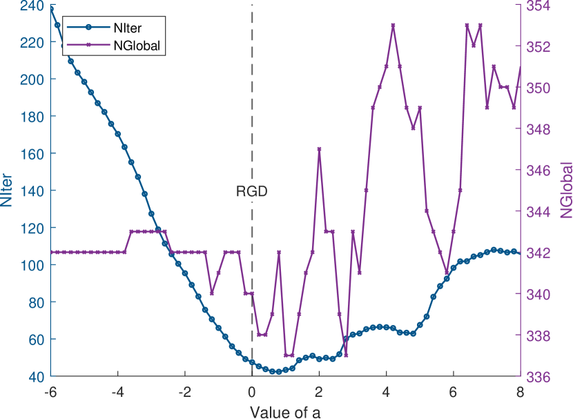
(a) TGP-A-R with different $a$ in (Case 1)

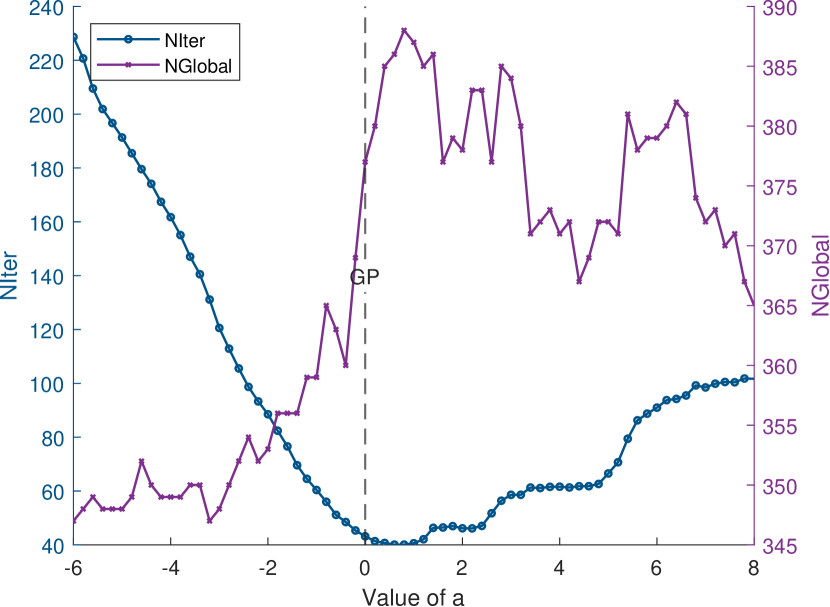
(b) TGP-A-E with different $a$ in (Case 1)

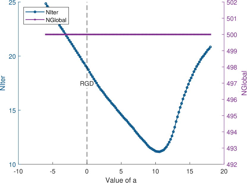
(c) TGP-A-R with different $a$ in (Case 2)

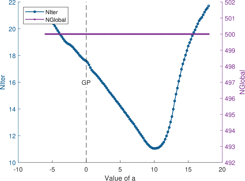
(d) TGP-A-E with different $a$ in (Case 2)

Figure 3. Results of (Exp 1) for Example 9.1

	Generate $\boldsymbol{A}$ as in (Case 1)				Generate $\boldsymbol{A}$ as in (Case 2)
Algorithm	NIter	Time	NGlobal	NFail	NIter	Time	NGlobal	NFail
TGP-A-R	43.0	0.0066	342	0	18.2	0.0037	500	0
TGP-NA-R	51.0	0.0073	348	0	34.5	0.0057	500	0
TGP-F-R	306.7	0.0296	339	0	9.6	0.0009	500	0
TGP-A-E	40.3	0.0054	387	0	17.0	0.0028	500	0
TGP-NA-E	48.8	0.0064	388	0	33.8	0.0051	500	0
TGP-F-E	303.4	0.0255	343	0	6.9	0.0006	500	0
SD	49.6	0.0605	346	0	17.0	0.0230	500	0
CG	34.0	0.0388	338	2	15.5	0.0177	500	0
BFGS	14.4	0.0399	336	0	10.4	0.0208	500	0

Table 2. Results of (Exp 2) for Example 9.1

Example 9.2.

We now consider the jointly approximate symmetric matrix diagonalization (JAMD-S) problem [46, 77, 48] on $\mathbf{St}(r,n)$:

$$\min\ f(\boldsymbol{X})=-\sum\limits_{\ell=1}^{L}\left\|\textbf{\operator@font\bf diag}\left(\boldsymbol{X}^{{\sf T}}\boldsymbol{A}^{(\ell)}\boldsymbol{X}\right)\right\|^{2},\ \ \boldsymbol{X}\in\mathbf{St}(r,n).$$ (71)

Here $\boldsymbol{A}^{(\ell)}\in\mathop{\operator@font\bf symm}\left(\mathbb{R}^{n\times n}\right)$ for all $\ell$, and $\textbf{\operator@font\bf diag}\left(\boldsymbol{W}\right)\stackrel{{\scriptstyle\sf def}}{{=}}(W_{11},W_{22},\ldots,W_{rr})^{{\sf T}}$ represents the vector composed of the diagonal elements of a matrix $\boldsymbol{W}\in\mathbb{R}^{r\times r}$. In the two experiments (Exp 1) and (Exp 2) for this problem, we still randomly generate 500 random instances in each experiment. The parameters maxiter and maxtime are set to $10^{4}$ and 2 seconds, respectively. For all instances, we set $n=3$, $r=2$ and $L=3$. In each instance, the initial point $\boldsymbol{X}_{0}$ is generated in the same way as in Example 9.1: $\boldsymbol{X}_{0}=\mathcal{P}_{\mathbf{St}(r,n)}(\texttt{randn}(n,r))$. For the matrices $\boldsymbol{A}^{(\ell)}$, we first generate an orthogonal matrix $\boldsymbol{Q}=\mathcal{P}_{\mathbf{O}_{n}}(\texttt{randn}(n,n))$, diagonal matrices $\boldsymbol{D}^{(\ell)}=\texttt{diag}({\texttt{randn}(n,1)})$, and small noise matrices $\boldsymbol{E}^{(\ell)}=0.01\cdot\mathop{\operator@font sym}\left(\texttt{randn}(n,r)\right)$ for all $\ell$, and then generate $\boldsymbol{A}^{(\ell)}=\boldsymbol{Q}^{{\sf T}}\boldsymbol{D}^{(\ell)}\boldsymbol{Q}+\boldsymbol{E}^{(\ell)}$. Due to the existence of the random noise matrices $\boldsymbol{E}^{(\ell)}$, the global minimum of this problem is unknown. Thus, we compare the quality of final iteration via NSuper, as previously discussed.

In the first experiment, to observe the influence of the normal component $\hat{\boldsymbol{H}}_{k}$, which depends on the value $a$ in (69), we set the baseline algorithm to be the TGP-A algorithm with $a=0$ to compute NSuper. To be more specific, in Figure 4(a), NSuper is computed by setting the baseline algorithm as the TGP-A-R algorithm with $a=0$ (the Riemannian gradient descent method). In Figure 4(b), we set the baseline algorithm as the TGP-A-E with $a=0$ (the classical gradient projection algorithm). We obtain similar results as in Footnote 21, where NIter and NSuper change significantly as $a$ changes.

In the second experiment, we set $a=2$ for TGP-$\ast$-R algorithms, and $a=5$ for TGP-$\ast$-E algorithms. The stepsizes of TGP-F-R and TGP-F-E are set as $0.02$ and $0.1$, respectively. The retraction-based algorithm SD is selected as the baseline algorithm to compute NSuper for all algorithms. The overall results of 500 randomly generated instances are shown in Table 3. We observe that TGP-NA-R can find better solution in many more cases. Moreover, TGP-F-E is the fastest one.

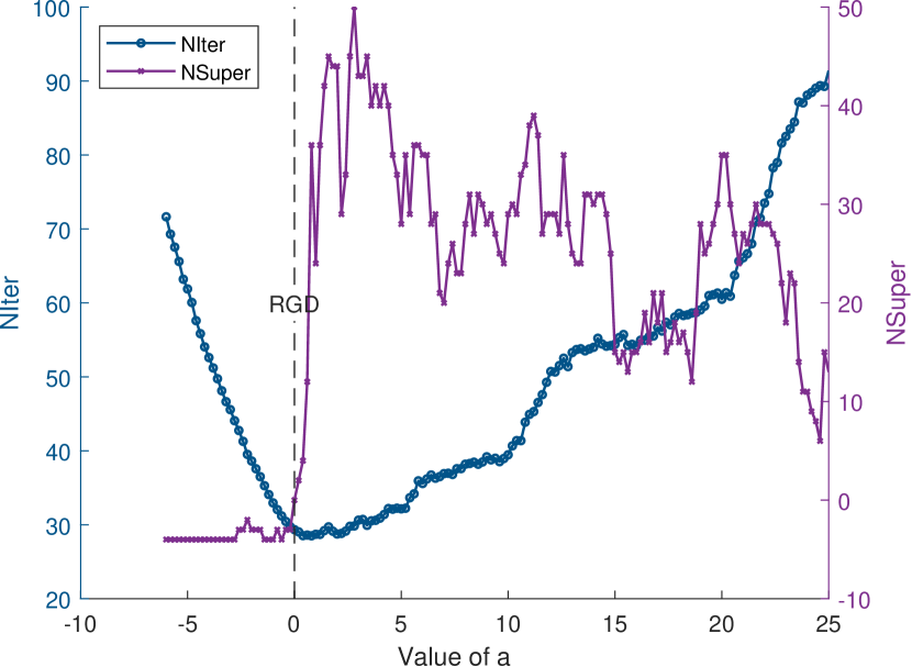
(a) TGP-A-R with different $a$

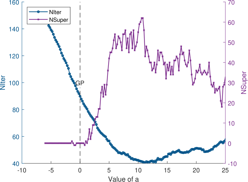
(b) TGP-A-E with different $a$

Figure 4. Results of (Exp 1) for Example 9.2

Algorithm	NIter	Time	NSuper (than SD)	NFail
TGP-A-R	28.8	0.0066	42	0
TGP-NA-R	39.4	0.0084	44	0
TGP-F-R	194.1	0.0247	-8	0
TGP-A-E	56.6	0.0120	36	0
TGP-NA-E	41.3	0.0071	39	0
TGP-F-E	51.4	0.0059	-7	0
SD	32.2	0.0397	0	0
CG	29.6	0.0340	-11	2
BFGS	12.0	0.0281	1	0

Table 3. Results of (Exp 2) for Example 9.2

Example 9.3.

We now further consider the following jointly approximate symmetric tensor diagonalization (JATD-S) problem [46, 77, 48] on $\mathbf{St}(r,n)$:

$$\min\ f(\boldsymbol{X})=-\sum\limits_{\ell=1}^{L}\left\|\textbf{\operator@font\bf diag}\left(\boldsymbol{\mathcal{A}}^{(\ell)}\mathop{\bullet_{1}}\boldsymbol{X}^{{\sf T}}\mathop{\bullet_{2}}\boldsymbol{X}^{{\sf T}}\mathop{\bullet_{3}}\boldsymbol{X}^{{\sf T}}\right)\right\|^{2},\ \ \boldsymbol{X}\in\mathbf{St}(r,n),$$ (72)

where $\boldsymbol{\mathcal{A}}^{(\ell)}\in\mathbb{R}^{n\times n\times n}$ is a $3$rd order symmetric tensor, and $\textbf{\operator@font\bf diag}\left(\boldsymbol{\mathcal{W}}\right)\stackrel{{\scriptstyle\sf def}}{{=}}(W_{111},W_{222},\ldots,W_{rrr})^{{\sf T}}$ represents the vector composed of the diagonal elements of a tensor $\boldsymbol{\mathcal{W}}\in\mathbb{R}^{r\times r\times r}$. We fix $n=3,r=2$ and $L=1$. The parameters maxiter and maxtime are set to $10^{4}$ and 5 seconds, respectively. In each random instance, we generate the initial point $\boldsymbol{X}_{0}$ as in Example 9.2, and $\boldsymbol{\mathcal{A}}^{(\ell)}=\texttt{symmetrize}(\texttt{tensor}(\texttt{randn}(n,n,n)))$. It can be seen that the global minimum of problem (72) is unknown. Therefore, we use the same strategy for setting the baseline algorithm as in Example 9.2. The results of (Exp 1) and (Exp 2) are presented in Figure 5 and Table 4, respectively. In the first experiment, we can still observe similar results: NSuper and NIter vary as $a$ changes. Especially, compared to the the case where $a=0$, slightly large $a$ may enhance the performance of the TGP-A algorithms. In the second experiment, we set $a=3$ for TGP-$\ast$-R algorithms, and $a=4$ for TGP-$\ast$-E algorithms. The stepsizes of TGP-F-R and TGP-F-E are set as 0.02 and 0.05, respectively. It can be seen that TGP-NA-E can find many more better solutions compared to other algorithms, and BFGS is the fastest one in this problem.

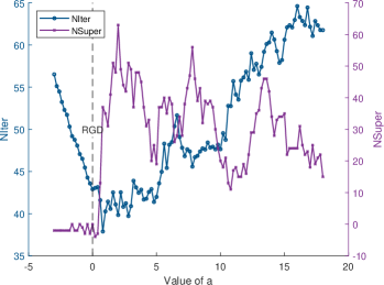
(a)

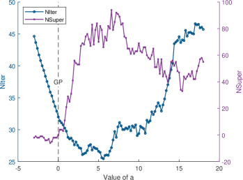
(b)

Figure 5. Results of (Exp 1) for Example 9.3

Algorithm	NIter	Time	NSuper (than SD)	NFail
TGP-A-R	42.1	0.1547	49	0
TGP-NA-R	52.9	0.1949	56	0
TGP-F-R	205.2	0.4367	-9	11
TGP-A-E	45.9	0.1681	54	0
TGP-NA-E	33.7	0.0999	64	0
TGP-F-E	79.0	0.1657	-6	0
SD	52.3	0.1491	0	0
CG	43.0	0.1263	-17	6
BFGS	13.7	0.0529	-4	0

Table 4. Results of (Exp 2) for Example 9.3

From the above numerical experiments in Examples 9.1, 9.2 and 9.3, we observe that the performance of TGP algorithms is significantly influenced by the normal component of $\boldsymbol{H}_{k}$, such as the value of $a$ in (69). With an appropriate normal component, the TGP algorithms can obtain better numerical performance compared with the retraction-based ones. In particular, in the case of Example 9.3, where the landscape of the optimization problem is more complex than Examples 9.1 and 9.2, the advantage of the TGP algorithms in terms of the quality of the final iteration becomes more obvious. Moreover, from Tables 2, 3 and 4, we observe that within the TGP algorithms, as the landscape of the optimization problem becomes more complex, the advantage of nonmonotone Armijo stepsizes over monotone ones also increases.

Remark 9.4.

In Tables 2 and 3, it is evident that the execution time of TGP algorithms is significantly shorter than that of the retraction-based algorithms, despite their similar number of iterations (NIter). However, this phenomenon is not observed in Table 4. This is due to that the implementation of the retraction in manopt costs much more time compared to the projection utilized in our TGP algorithms. When it comes to the optimization problem in Example 9.3, which is more complex, the time difference mentioned earlier is less compared to other computations, including the evaluation of the objective value and gradient. As a result, in Table 4, the execution time and NIter for all algorithms exhibit a nearly proportional relationship.

10. Conclusions

In this paper, using the projection onto a compact matrix manifold, we propose a general TGP algorithmic framework to solve problem (1). Our framework not only covers numerous existing algorithms in the literature, but also encompasses several new special cases. Notably, this generalization is also different from the classical retraction-based algorithmic framework, as illustrated in Figure 1. For this new general algorithmic framework with various stepsizes including the Armijo stepsize, the nonmonotone Armijo stepsize, and the fixed stepsize, we establish their weak convergence and convergence rate. A key aspect of our analysis is the exploration of the projection onto a compact submanifold, which is important for our convergence results and may also be of independent interest. Furthermore, we prove the global convergence of our algorithmic framework via the Łojasiewicz property. Prior to this paper, to our knowledge, the global convergence of the Zhang-Hager type nonmonotone Armijo stepsize has not been established for nonconvex problems in the literature, even in Euclidean space.

In the end, we would like to emphasize that, our convergence analysis can be easily extended to more general projection-based line-search algorithms (4). To be more specific, the weak convergence and convergence rate can be established if the tangent component of the search direction $\boldsymbol{H}_{k}$ is equivalent to the Riemannian gradient, i.e., if $\boldsymbol{\tilde{H}}_{k}$ satisfies (28) and (29). Moreover, global convergence under Łojasiewicz property holds if the normal component of $\boldsymbol{H}_{k}$ is not too large, i.e., there exists $\delta>0$ such that $\tau_{k}\|\boldsymbol{\hat{H}}_{k}\|<\varrho_{*}-\delta$.

References

- [1] P.-A. Absil, C. G. Baker, and K. A. Gallivan, Trust-region methods on Riemannian manifolds, Foundations of Computational Mathematics, 7 (2007), pp. 303–330.
- [2] P.-A. Absil, R. Mahony, and B. Andrews, Convergence of the iterates of descent methods for analytic cost functions, SIAM Journal on Optimization, 16 (2005), pp. 531–547.
- [3] P.-A. Absil, R. Mahony, and R. Sepulchre, Optimization algorithms on matrix manifolds, Princeton University Press, 2009.
- [4] P.-A. Absil and J. Malick, Projection-like retractions on matrix manifolds, SIAM Journal on Optimization, 22 (2012), pp. 135–158.
- [5] A. Anandkumar, R. Ge, D. Hsu, S. M. Kakade, and M. Telgarsky, Tensor decompositions for learning latent variable models, Journal of Machine Learning Research, 15 (2014), pp. 2773–2832.
- [6] L. Armijo, Minimization of functions having Lipschitz continuous first partial derivatives, Pacific Journal of mathematics, 16 (1966), pp. 1–3.
- [7] B. W. Bader, T. G. Kolda, et al., Matlab tensor toolbox version 3.0-dev. Available online, Aug. 2017, https://gitlab.com/tensors/tensor_toolbox.
- [8] M. V. Balashov, Gradient Projection Method on Matrix Manifolds, Computational Mathematics and Mathematical Physics, 60 (2020), pp. 1403–1411.
- [9] N. Bansal, X. Chen, and Z. Wang, Can we gain more from orthogonality regularizations in training deep networks?, Advances in Neural Information Processing Systems, 31 (2018).
- [10] E. Batzies, K. Hüper, L. Machado, and F. S. Leite, Geometric mean and geodesic regression on Grassmannians, Linear Algebra and its Applications, 466 (2015), pp. 83–101.
- [11] A. Beck, First-Order Methods in Optimization, Society for Industrial and Applied Mathematics, Philadelphia, PA, 2017.
- [12] T. Bendokat, R. Zimmermann, and P.-A. Absil, A Grassmann manifold handbook: Basic geometry and computational aspects, arXiv preprint arXiv:2011.13699, (2020).
- [13] G. C. Bento, O. P. Ferreira, and J. G. Melo, Iteration-complexity of gradient, subgradient and proximal point methods on Riemannian manifolds, Journal of Optimization Theory and Applications, 173 (2017), pp. 548–562.
- [14] S. Bonettini and M. Prato, New convergence results for the scaled gradient projection method, Inverse Problems, 31 (2015), p. 095008.
- [15] S. Bonettini, R. Zanella, and L. Zanni, A scaled gradient projection method for constrained image deblurring, Inverse problems, 25 (2008), p. 015002.
- [16] C. Botsaris, Constrained optimization along geodesics, Journal of mathematical analysis and applications, 79 (1981), pp. 295–306.
- [17] N. Boumal, An introduction to optimization on smooth manifolds, Cambridge University Press, 2023.
- [18] N. Boumal and P.-A. Absil, Low-rank matrix completion via preconditioned optimization on the Grassmann manifold, Linear Algebra and its Applications, 475 (2015), pp. 200–239.
- [19] N. Boumal, P.-A. Absil, and C. Cartis, Global rates of convergence for nonconvex optimization on manifolds, IMA Journal of Numerical Analysis, 39 (2019), pp. 1–33.
- [20] N. Boumal, B. Mishra, P.-A. Absil, and R. Sepulchre, Manopt, a Matlab toolbox for optimization on manifolds, Journal of Machine Learning Research, 15 (2014), pp. 1455–1459.
- [21] J. Chen and Y. Saad, On the tensor SVD and the optimal low rank orthogonal approximation of tensors, SIAM Journal on Matrix Analysis and Applications, 30 (2009), pp. 1709–1734.
- [22] A. Cichocki, D. Mandic, L. D. Lathauwer, G. Zhou, Q. Zhao, C. Caiafa, and H. A. PHAN, Tensor decompositions for signal processing applications: From two-way to multiway component analysis, IEEE Signal Processing Magazine, 32 (2015), pp. 145–163.
- [23] F. H. Clarke, R. J. Stern, and P. R. Wolenski, Proximal smoothness and the lower-c2 property, J. Convex Anal, 2 (1995), pp. 117–144.
- [24] P. Comon and C. Jutten, eds., Handbook of Blind Source Separation, Academic Press, Oxford, 2010.
- [25] S. Crisci, F. Porta, V. Ruggiero, and L. Zanni, On the convergence properties of scaled gradient projection methods with non-monotone Armijo–like line searches, ANNALI DELL’UNIVERSITA’DI FERRARA, (2022), pp. 1–34.
- [26] Y.-H. Dai, On the nonmonotone line search, Journal of Optimization Theory and Applications, 112 (2002), pp. 315–330.
- [27] M. P. Do Carmo, Differential geometry of curves and surfaces: revised and updated second edition, Courier Dover Publications, 2016.
- [28] A. Edelman, T. A. Arias, and S. T. Smith, The geometry of algorithms with orthogonality constraints, SIAM Journal on Matrix Analysis and Applications, 20 (1998), pp. 303–353.
- [29] D. Gabay, Minimizing a differentiable function over a differential manifold, Journal of Optimization Theory and Applications, 37 (1982), pp. 177–219.
- [30] B. Gao, X. Liu, X. Chen, and Y.-X. Yuan, A new first-order algorithmic framework for optimization problems with orthogonality constraints, SIAM Journal on Optimization, 28 (2018), pp. 302–332.
- [31] B. Gao, N. T. Son, and T. Stykel, Optimization on the symplectic Stiefel manifold: Sr decomposition-based retraction and applications, arXiv preprint arXiv:2211.09481, (2022).
- [32] G. H. Golub and C. F. Van Loan, Matrix Computations, Johns Hopkins University Press, 4th ed., 2013.
- [33] N. J. Higham, Functions of matrices: theory and computation, vol. 104, SIAM, 2008.
- [34] R. A. Horn and C. R. Johnson, Matrix Analysis, Cambridge University Press, 2012.
- [35] J. Hu, X. Liu, Z.-W. Wen, and Y.-X. Yuan, A brief introduction to manifold optimization, Journal of the Operations Research Society of China, 8 (2020), pp. 199–248.
- [36] J. Hu, A. Milzarek, Z. Wen, and Y. Yuan, Adaptive quadratically regularized newton method for Riemannian optimization, SIAM Journal on Matrix Analysis and Applications, 39 (2018), pp. 1181–1207.
- [37] S. Hu and K. Ye, Linear convergence of an alternating polar decomposition method for low rank orthogonal tensor approximations, Mathematical Programming, 199 (2023), pp. 1305–1364.
- [38] W. Huang, P.-A. Absil, and K. A. Gallivan, A Riemannian BFGS method without differentiated retraction for nonconvex optimization problems, SIAM Journal on Optimization, 28 (2018), pp. 470–495.
- [39] W. Huang, K. A. Gallivan, and P.-A. Absil, A broyden class of quasi-newton methods for Riemannian optimization, SIAM Journal on Optimization, 25 (2015), pp. 1660–1685.
- [40] B. Jiang and Y.-H. Dai, A framework of constraint preserving update schemes for optimization on Stiefel manifold, Mathematical Programming, 153 (2015), pp. 535–575.
- [41] M. Journée, Y. Nesterov, P. Richtárik, and R. Sepulchre, Generalized power method for sparse principal component analysis, Journal of Machine Learning Research, 11 (2010).
- [42] T. G. Kolda and B. W. Bader, Tensor decompositions and applications, SIAM Review, 51 (2009), pp. 455–500.
- [43] S. Krantz and H. Parks, A Primer of Real Analytic Functions, Birkhäuser Boston, 2002.
- [44] R. Lai and S. J. Osher, A splitting method for orthogonality constrained problems, Journal of Scientific Computing, 58 (2014), pp. 431–449.
- [45] S. law Lojasiewicz, Ensembles semi-analytiques, IHES notes, (1965).
- [46] J. Li, K. Usevich, and P. Comon, Globally convergent Jacobi-type algorithms for simultaneous orthogonal symmetric tensor diagonalization, SIAM Journal on Matrix Analysis and Applications, 39 (2018), pp. 1–22.
- [47] J. Li, K. Usevich, and P. Comon, On approximate diagonalization of third order symmetric tensors by orthogonal transformations, Linear Algebra and its Applications, 576 (2019), pp. 324–351.
- [48] J.-Z. Li and S.-Z. Zhang, Polar decomposition-based algorithms on the product of Stiefel manifolds with applications in tensor approximation, Journal of the Operations Research Society of China, (2023), pp. 1–47.
- [49] R.-C. Li, New perturbation bounds for the unitary polar factor, SIAM Journal on Matrix Analysis and Applications, 16 (1995), pp. 327–332.
- [50] X. Li, S. Chen, Z. Deng, Q. Qu, Z. Zhu, and A. Man-Cho So, Weakly convex optimization over Stiefel manifold using Riemannian subgradient-type methods, SIAM Journal on Optimization, 31 (2021), pp. 1605–1634.
- [51] S. Ling, Improved performance guarantees for orthogonal group synchronization via generalized power method, SIAM Journal on Optimization, 32 (2022), pp. 1018–1048.
- [52] H. Liu, A. M.-C. So, and W. Wu, Quadratic optimization with orthogonality constraint: Explicit łojasiewicz exponent and linear convergence of retraction-based line-search and stochastic variance-reduced gradient methods, Mathematical Programming, 178 (2019), pp. 215–262.
- [53] H. Liu, M.-C. Yue, and A. Man-Cho So, On the estimation performance and convergence rate of the generalized power method for phase synchronization, SIAM Journal on Optimization, 27 (2017), pp. 2426–2446.
- [54] S. Łojasiewicz, Sur la géométrie semi- et sous-analytique, Annales de l’institut Fourier, 43 (1993), pp. 1575–1595.
- [55] D. G. Luenberger, Y. Ye, et al., Linear and nonlinear programming, vol. 2, Springer, 1984.
- [56] J. R. Munkres, Topology: a first course, Prentice-Hall, 1974.
- [57] Y. Nesterov, Lectures on Convex Optimization, vol. 137 of Springer Optimization and Its Applications, Springer International Publishing, Cham, 2018.
- [58] J. Nocedal and S. J. Wright, Numerical Optimization, Springer Series in Operations Research, Springer, New York, 2006.
- [59] H. Oviedo, Global convergence of riemannian line search methods with a zhang-hager-type condition, Numerical Algorithms, 91 (2022), pp. 1183–1203.
- [60] H. Oviedo, A worst-case complexity analysis for Riemannian non-monotone line-search methods, (2023).
- [61] H. Oviedo and O. Dalmau, A scaled gradient projection method for minimization over the Stiefel manifold, in Mexican International Conference on Artificial Intelligence, Springer, 2019, pp. 239–250.
- [62] H. Oviedo, O. Dalmau, and H. Lara, Two adaptive scaled gradient projection methods for Stiefel manifold constrained optimization, Numerical Algorithms, 87 (2021), pp. 1107–1127.
- [63] H. Oviedo, H. Lara, and O. Dalmau, A non-monotone linear search algorithm with mixed direction on Stiefel manifold, Optimization Methods and Software, 34 (2019), pp. 437–457.
- [64] L. Qi and Z. Luo, Tensor analysis: Spectral theory and special tensors, SIAM, 2017.
- [65] L. Qi, F. Wang, and Y. Wang, Z-eigenvalue methods for a global polynomial optimization problem, Mathematical Programming, 118 (2009), pp. 301–316.
- [66] H. Sato and T. Iwai, Optimization algorithms on the Grassmann manifold with application to matrix eigenvalue problems, Japan Journal of Industrial and Applied Mathematics, 31 (2014), pp. 355–400.
- [67] R. Schneider and A. Uschmajew, Convergence results for projected line-search methods on varieties of low-rank matrices via łojasiewicz inequality, SIAM Journal on Optimization, 25 (2015), pp. 622–646.
- [68] Z. Sheng, W. Yang, and J. Wen, A Riemannian gradient ascent algorithm with applications to orthogonal approximation problems of symmetric tensors, Applied Numerical Mathematics, 182 (2022), pp. 235–247.
- [69] M. Shub, Some remarks on dynamical systems and numerical analysis, Proc. VII ELAM.(L. Lara-Carrero and J. Lewowicz, eds.), Equinoccio, U. Simón Bolıvar, Caracas, (1986), pp. 69–92.
- [70] N. D. Sidiropoulos, L. De Lathauwer, X. Fu, K. Huang, E. E. Papalexakis, and C. Faloutsos, Tensor decomposition for signal processing and machine learning, IEEE Transactions on Signal Processing, 65 (2017), pp. 3551–3582.
- [71] S. T. Smith, Geometric optimization methods for adaptive filtering, Harvard University, 1993.
- [72] S. T. Smith, Optimization techniques on Riemannian manifolds, Fields Institute Communications, 3 (1994).
- [73] E. Stiefel, Richtungsfelder und fernparallelismus in n-dimensionalen mannigfaltigkeiten, Commentarii Mathematici Helvetici, 8 (1935), pp. 305–353.
- [74] P. L. Toint, An assessment of nonmonotone linesearch techniques for unconstrained optimization, SIAM Journal on Scientific Computing, 17 (1996), pp. 725–739.
- [75] N. T. Trendafilov and R. A. Lippert, The multimode procrustes problem, Linear algebra and its applications, 349 (2002), pp. 245–264.
- [76] A. Uschmajew, A new convergence proof for the higher-order power method and generalizations, Pac. J. Optim., 11 (2015), pp. 309–321.
- [77] K. Usevich, J. Li, and P. Comon, Approximate matrix and tensor diagonalization by unitary transformations: convergence of Jacobi-type algorithms, SIAM Journal on Optimization, 30 (2020), pp. 2998–3028.
- [78] K. Usevich and I. Markovsky, Optimization on a Grassmann manifold with application to system identification, Automatica, 50 (2014), pp. 1656–1662.
- [79] J. Wang, Y. Chen, R. Chakraborty, and S. X. Yu, Orthogonal convolutional neural networks, in Proceedings of the IEEE/CVF conference on computer vision and pattern recognition, 2020, pp. 11505–11515.
- [80] Z. Wen, A. Milzarek, M. Ulbrich, and H. Zhang, Adaptive regularized self-consistent field iteration with exact hessian for electronic structure calculation, SIAM Journal on Scientific Computing, 35 (2013), pp. A1299–A1324.
- [81] Z. Wen, C. Yang, X. Liu, and Y. Zhang, Trace-penalty minimization for large-scale eigenspace computation, Journal of Scientific Computing, 66 (2016), pp. 1175–1203.
- [82] Z. Wen and W. Yin, A feasible method for optimization with orthogonality constraints, Mathematical Programming, 142 (2013), pp. 397–434.
- [83] N. Xiao, X. Liu, and Y. xiang Yuan, A class of smooth exact penalty function methods for optimization problems with orthogonality constraints, Optimization Methods and Software, 37 (2020), pp. 1205 – 1241.
- [84] N. Xiao, X. Liu, and Y.-x. Yuan, Exact penalty function for norm minimization over the Stiefel manifold, SIAM Journal on Optimization, 31 (2021), pp. 3097–3126.
- [85] Y. Yang, Globally convergent optimization algorithms on Riemannian manifolds: Uniform framework for unconstrained and constrained optimization, Journal of Optimization Theory and Applications, 132 (2007), pp. 245–265.
- [86] Y. Yang, The epsilon-alternating least squares for orthogonal low-rank tensor approximation and its global convergence, SIAM Journal on Matrix Analysis and Applications, 41 (2020), pp. 1797–1825.
- [87] D. Zhang and S. Davanloo Tajbakhsh, Riemannian stochastic variance-reduced cubic regularized newton method for submanifold optimization, Journal of Optimization Theory and Applications, 196 (2023), pp. 324–361.
- [88] H. Zhang and W. W. Hager, A nonmonotone line search technique and its application to unconstrained optimization, SIAM journal on Optimization, 14 (2004), pp. 1043–1056.
- [89] H. Zhang, S. J Reddi, and S. Sra, Riemannian svrg: Fast stochastic optimization on Riemannian manifolds, Advances in Neural Information Processing Systems, 29 (2016).
- [90] H. Zhang and S. Sra, First-order methods for geodesically convex optimization, in Conference on Learning Theory, PMLR, 2016, pp. 1617–1638.
- [91] J. Zhang and S. Zhang, A cubic regularized newton’s method over Riemannian manifolds, arXiv preprint arXiv:1805.05565, (2018).
- [92] L. Zhu, J. Wang, and A. M.-C. So, Orthogonal group synchronization with incomplete measurements: Error bounds and linear convergence of the generalized power method, arXiv preprint arXiv:2112.06556, (2021).