SemanticFormer: Holistic and Semantic Traffic Scene Representation for Trajectory Prediction using Knowledge Graphs

Abstract

Trajectory prediction in autonomous driving relies on accurate representation of all relevant contexts of the driving scene including traffic participants, road topology, traffic signs as well as their semantic relations to each other. Despite increased attention to this issue, most approaches in trajectory prediction do not consider all of these factors sufficiently. This paper describes a method SemanticFormer to predict multimodal trajectories by reasoning over a semantic traffic scene graph using a hybrid approach. We extract high-level information in the form of semantic meta-paths from a knowledge graph which is then processed by a novel pipeline based on multiple attention mechanisms to predict accurate trajectories. The proposed architecture comprises a hierarchical heterogeneous graph encoder, which can capture spatio-temporal and relational information across agents and between agents and road elements, and a predictor that fuses the different encodings and decodes trajectories with probabilities. Finally, a refinement module evaluates permitted meta-paths of trajectories and speed profiles to obtain final predicted trajectories. Evaluation of the nuScenes benchmark demonstrates improved performance compared to the state-of-the-art methods.

I INTRODUCTION

Autonomous vehicles are recognized as a promising solution to address critical challenges such as road safety, traffic congestion, and energy optimization. A crucial task towards the realization of autonomous driving vision is motion prediction. It involves determining a set of spatial coordinates that represent the predicted movement of a given agent within a future time window. However, motion prediction is a challenging task due to various contextual factors such as the difficulty of intentions prediction, the complex interactions of traffic participants, the intricate road topology, comprising lanes, lane dividers, and pedestrian crossings, as well as adherence to traffic regulations. Therefore, state-of-the-art approaches try to use various representations for the traffic scene such as raster-based [1, 2], or graph-based [3, 4] to capture and utilize contextual information sufficiently.

Figure 1: Schematic illustration of the traffic scene. The input information of SemanticFormer includes meta-paths, map topology, agent-agent, and agent-map. These graphs are in the form of a heterogeneous graph enriched with semantic relation types.

Recent work applies a knowledge graph to represent the heterogeneous context in traffic scenes [5]. So far, this representation has not been used for trajectory prediction. Because knowledge graphs can represent different entities and their relations as shown in Figure 1, which is important in driving scene processing, We propose a novel hybrid approach that can represent heterogeneous information of static and dynamic elements of a traffic scene together with their semantic relationships. In addition, the proposed architecture comprises an attention mechanism for leveraging the semantic relationships and dependencies between traffic agents and road elements for accurate multimodal trajectory prediction. Our main contributions are:

• We propose a symbolic approach that can represent heterogeneous information of static and dynamic elements of a traffic scene with their semantic relationships.

• We propose a hybrid architecture with attention mechanisms that is able to model the semantic relationships and dependencies between traffic agents and road elements for accurate multi-modal trajectory prediction.

• We evaluate our method on the nuScenes dataset[6] and perform extensive ablation studies on different heterogeneous graph operators and point out their limitations when applied to complex knowledge graphs.

Figure 2: Overview of our approach: Data Representation models the static map information and dynamic agents interaction by a holistic knowledge graph. Scene Graph Encoder extracts meta-paths and generates holistic latent representation for agents and lanes. Probability Predictor fuses the encodings and outputs trajectory candidates. Prediction Refinement uses anchor paths and speed profiles to evaluate trajectories and generates final predictions

II RELATED WORK

Raster-based representation. Approaches using raster-based representation of the map and agents are some of the first neural-network based methods for trajectory prediction. They encode the whole traffic scene into birds-eye-view images with a number of channels. The channels are used to represent the various kinds of road structures and agents in a scene [1, 2, 7]. On top of the raster-representations, convolutional neural networks (CNN) are usually applied to learn a representation of the map and agents. Drawback of these models is that they do not have access to high-level information and need to learn from raw pixels. An alternative approach aims to estimate probability distribution heatmaps representing locations where agents could be at a fixed time horizon [8, 9, 10]. Meanwhile, raster-based approaches are further extended to generate multiple possible trajectories while also estimating their probabilities[1, 2, 8].

Graph-based representation. The next generation of trajectory prediction techniques represent scenes as vectors, polylines and graphs [4, 11, 12, 13, 14, 15, 16]. State-of-the-art approaches in this category leverage graphs as a means of data representation, operating thus in a higher level of abstraction. By eliminating the need for networks to learn from low-level pixels, these methods are anticipated to exhibit greater resilience in handling variances.

Methods like VectorNet [4] encode both map features and agent trajectories as polylines and then merge them with a global interaction graph. TNT [17] extends VectorNet and combines it with multiple target reference trajectory proposals sampled from the lanes to diversify the prediction points. A limitation of these approaches is that they usually only consider homogeneous graphs with one entity type and one relation type. Additional information like pedestrian crossings is often included with a flag.

Heterogeneous Graph representation. Methods for heterogeneous graphs, i.e. graphs with different entity types such as vehicles, bicycles or pedestrians and relation types such as agent-to-lane or agent-to-agent, are recently proposed in [18, 19, 20, 21]. On the other hand [15, 22] use high-level representations, where single nodes represent whole entities, like vehicles or lanes. For such high-level representations, heterogeneous graphs are employed to capture different types of nodes and edges that arise. Our approach extends these heterogeneous graph-based representation methods by using formal ontologies to represent the rich semantics of the domain. These enable the establishment of expressive knowledge graphs which can comprise prior knowledge, and contextual information from diverse sources such as weather, traffic, etc.

Attention mechanisms [23] are widely used to learn to which data to pay attention to in the trajectory prediction task. This mechanism is used in raster-based approaches [24, 25, 26, 27, 28], in vector- or graph-based approaches [29, 30, 31, 32, 33, 34] and in map-free approaches [35]. A hierarchical vector transformer based approach is presented in [36] that consists of a local context feature encoding followed by global message passing among agent-centric local regions.

Goal- or intention conditioned systems sample goal candidates and predict trajectories conditioned on them [37, 38, 34, 17, 39]. Authors in [40] use grid based policy learning via maximum entropy inverse reinforcement learning to condition trajectory forecasts.

Anchor trajectories. Approaches that leverage a fixed set of anchors corresponding to permitted and possible trajectories are presented in [41, 2]. [13] presents a method to learn latent representations of anchor trajectories. Our approach takes up the idea of anchor trajectories and develops them further into meta paths as described below.

Figure 3: Illustration of traffic scene ontologies[5]: Agent Ontology defines agent attributes like category, speed, position, and trajectory, and relationships to map like distance to lane, and path distance. Map Ontology defines map elements like lane snippet, lane slice, traffic light, etc., and relations within map elements like left/right lane, switch via double dashed line.

Interaction Modelling. A number of trajectory prediction approaches that consider the interaction between the agents are presented in  [34, 42]. We model these interaction more explicitly by defining specific relationships, e.g. if the vehicle might intersect or drive on the same lane, and attributes like the distance between two vehicles along the lane.

III METHODOLOGY

We represent the map and agent information with a knowledge graph. This enables us to explicitly model the various map elements like lanes, lane dividers, etc, and their semantic relations. It also allows for the modeling of diverse traffic agent types like cars, bicycles, etc., and their relations in driving situations such as whether two agents might interact, drive behind one another, or next to each other.

In the following, we describe a comprehensive architecture depicted in Figure 2, which uses a knowledge graph for predicting multimodal trajectories. The architecture begins by taking the scene graph $g_{i}$ as input and outputs multimodal trajectories for the target agent. Finally, the refinement module filters the predicted trajectories considering anchor paths and speed profiles to avoid failure cases. Each module of the architecture is explained in detail below.

III-A Ontology and Heterogeneous Scene Graph

We utilize ontologies to explicitly represent the abundance of information from traffic scenes[5]. Thus, based on the domain knowledge we model relationships between entities considered important for the task of trajectory prediction. Figure 3 illustrates the developed ontologies, encompassing various entity and relation types. The entity types are categorized into two groups: the first one, contains static map entities like lane types, boundaries, center lines and stop areas; whereas the second group contains dynamic agent entities like agent types, states, and bounding boxes. As for relation types, they fall into three groups: 1) between agents, which construct the semantic model through associations such as lateral, longitudinal, and intersecting, shown in figure 4(b) akin to the concepts presented in [22]; 2) between map elements, establishing lane connectivity and relationships between lanes and road infrastructure elements like stop areas, traffic lights, pedestrian crossings; and 3) relations between map elements and agents, utilizing probability projection to map agents onto road infrastructure.

Based on the designed ontology, we represent the scene by a directed heterogeneous scene graph $G=(V,E,\tau,\phi)$. This scene graph has nodes $v\in V$, with node types $\tau(v)$, and edges $(u,v)\in E$, with edge types $\phi(u,v)$. The edges are directed since they are based on properties of the knowledge graph.

III-B Problem Formulation for Trajectory Prediction

We assume that the perception part can provide detailed information about agent positions, and past motion as well as the HD map, we build the scene graph described in the previous section. Then, a sample of the dataset can be formed as $\left(g_{i},y_{i}\right)$ where $g_{i}$ is a sample scene graph with trajectory information, local map, and target identifier and $y_{i}$ is the ground truth future trajectory of the target. Both agent past trajectories and map information are represented hierarchically. And $g_{i}\in G$ covers the information within a given time horizon $\left\{-t_{h}+1,\cdots,0,1,\cdots,t_{f}\right\}$. We use $\mathbf{P}_{-t_{h}+1:0}^{i}=\left\{sp_{-t_{h}+2}^{i},sp_{-t_{h}+3}^{i},\ldots,sp_{0}^{i}\right\}$ to represent the participant node. Each scene participant node $sp_{t}^{i}$ is represented as $sp_{t}^{i}=\left[d_{t,s}^{i},d_{t,e}^{i},a^{i}\right]$, where $d_{t,s}^{i}$ and $d_{t,e}^{i}$ stands for previous and current time stamps scene participant locations, and $a^{i}$ represent other attributes related to current scene participant like velocity, acceleration, heading change rate and object type. For map information, we use $\mathbf{S}_{1:N}^{i}=\left\{s_{1}^{i},s_{2}^{i},\ldots,s_{N}^{i}\right\}$ to represent a lane snippet, where each $s_{n}^{i}$ represents a lane slice and $N$ represents the length of the given lane snippet. Each lane slice vector $s_{n}^{i}=\left[d_{n,s}^{i},d_{n,e}^{i},a_{i},d_{n,\mathrm{pre}}^{i}\right]$ adds $d_{n,\mathrm{pre}}^{i}$ to indicate the predecessor of the start point. To build the connection between lane snippets, we use $\mathbf{C}_{1:N}^{i}=\left\{c_{1}^{i},c_{2}^{i},\ldots,c_{N}^{i}\right\}$ representing a lane connector, where each $c_{n}^{i}$ encodes an ordered pose inside the lane connector and $N$ represents the length of lane connector.

Coordinates in the knowledge graph are initially in a global coordinate system. These are transformed separately into local, scene graph-specific coordinates, with the origin at the location of the target agent and the positive y-axis pointing along the facing direction of the target.

III-C Semantic Scene Graph Hierarchical Modelling

III-C1 Meta-Path Generation

We extract meta-paths that describe permitted and possible driving directions to navigate the target participant. Different meta-paths that model permitted lane changes and turns can be divided into three groups, which are the lane-changing, the entering lane connector, and the leaving lane connector situations.

(a) Meta-path Generation

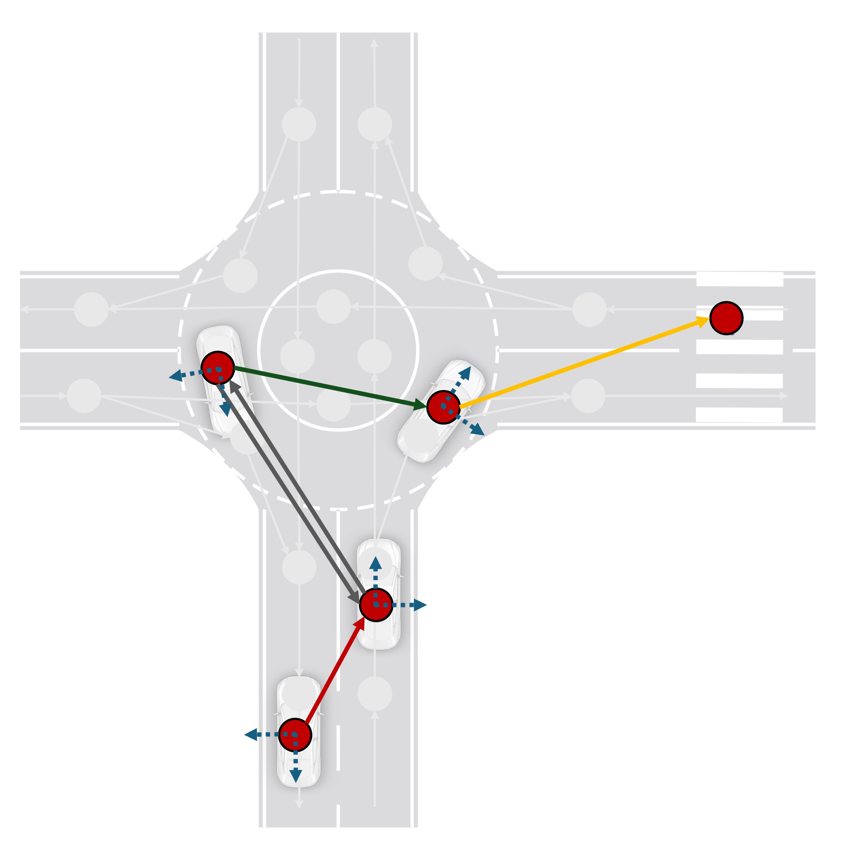
(b) Agent-Agent Interaction

Figure 4: (a) Illustration of the meta-path generation. (b) Illustration of the participant interaction graph: Characterized by edge types: Longitudinal(green), Intersecting(gray), Lateral(red), and Pedestrian(yellow).

Figure 4(a) gives a qualitative analysis of generated meta-paths. Specifically, we illustrate sample meta-paths below, such as lane changing 1, leaving connector 2, and entering connector cases 3, where $\Phi$ represents the meta-path.

$$\Phi_{0}=\mathbf{P}\stackrel{{\scriptstyle isOn}}{{\longrightarrow}}\mathbf{S}\stackrel{{\scriptstyle switchViaX}}{{\longrightarrow}}\mathbf{S}\stackrel{{\scriptstyle switchViaX}}{{\longrightarrow}}\mathbf{S}$$ (1)

$$\Phi_{1}=\mathbf{P}\stackrel{{\scriptstyle isOn}}{{\longrightarrow}}\mathbf{C}\stackrel{{\scriptstyle CconnectS}}{{\longrightarrow}}\mathbf{S}\stackrel{{\scriptstyle switchViaX}}{{\longrightarrow}}\mathbf{S}$$ (2)

$$\Phi_{2}=\mathbf{P}\stackrel{{\scriptstyle isOn}}{{\longrightarrow}}\mathbf{S}\stackrel{{\scriptstyle switchViaX}}{{\longrightarrow}}\mathbf{S}\stackrel{{\scriptstyle SconnectC}}{{\longrightarrow}}\mathbf{C}$$ (3)

III-C2 Agent Motion and Lane Encoder

This section introduces a spatio-temporal encoder. We process participants $\mathbf{P}^{i}$, lane snippets $\mathbf{S}_{1:N}^{i}$, and lane connectors $\mathbf{C}_{1:N}^{i}$ in a sequential manner using both a Graph Neural Network (GNN) and a Gated Recurrent Unit (GRU) layer. $p_{i}$, $s_{j}$ and $c_{z}$ are used to represent the encodings respectively. Further, inspired by LaneGCN[11], we merge the outcomes as shown in Figure 5. Equation 4 introduces lane information to the related agents while equation 5 and equation 6 add participant information to the related lanes and lane connectors.

$$p_{i}=p_{i}+\operatorname{CrossAtt}\left\{p_{i},[s_{j},c_{z}]\right\}$$ (4)

$$s_{j}=s_{j}+\operatorname{CrossAtt}\left\{s_{j},p_{i}\right\}$$ (5)

$$c_{z}=c_{z}+\operatorname{CrossAtt}\left\{c_{z},p_{i}\right\}$$ (6)

where $i\in\left\{1,\ldots,N_{\text{P}}\right\},j\in\left\{1,\ldots,N_{\text{LS }}\right\},z\in\left\{1,\ldots,N_{\text{LC }}\right\}$. These encodings are assigned to node attributes in $g_{i}$.

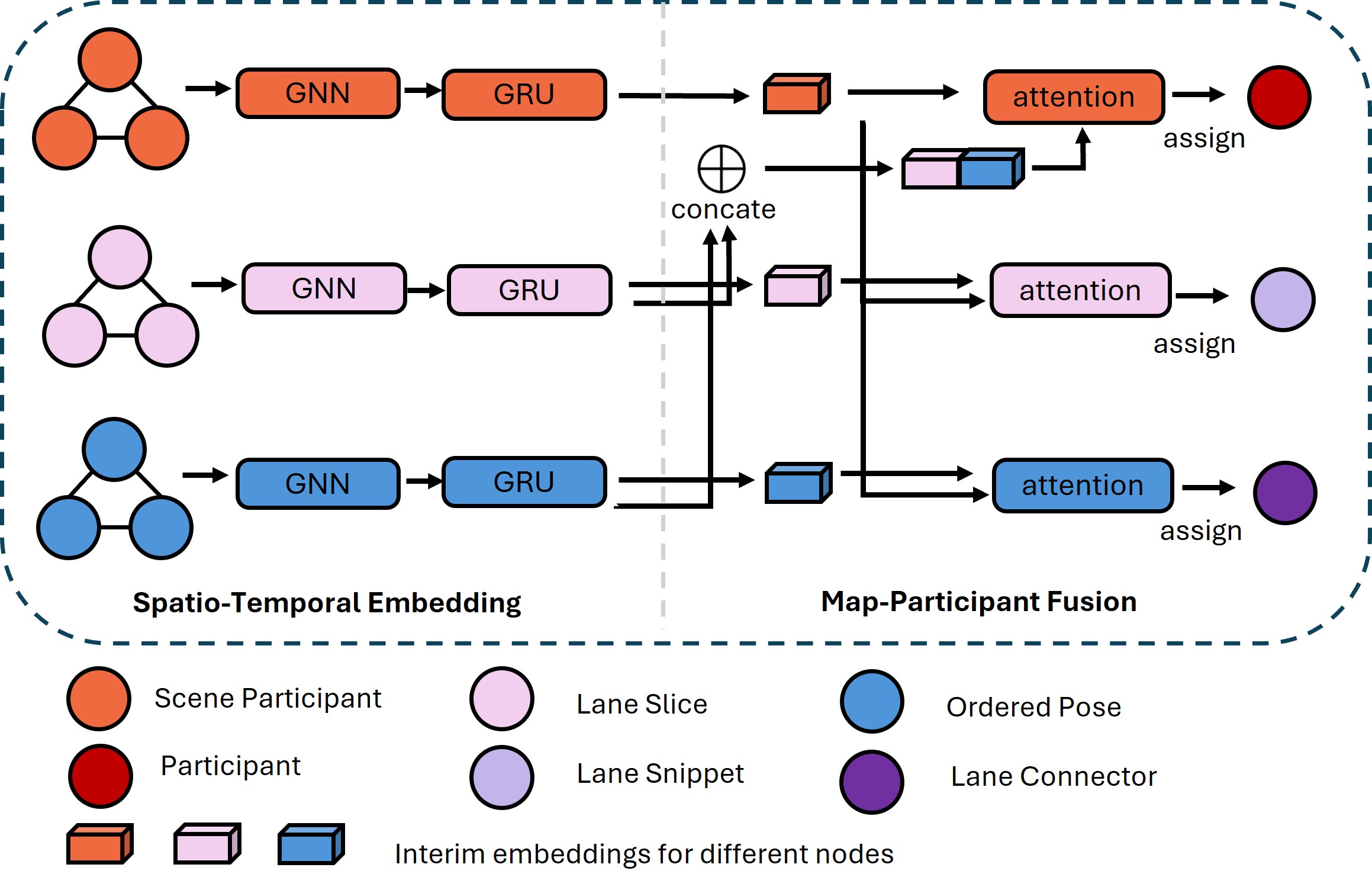
Figure 5: Illustration of agent motion and lane encoder: GNN and GRU extracts spatio-temporal information, attention mechanism models participants related lane

III-C3 Semantic Scene Graph Encoder

A heterogeneous graph operator is used to reason over the given scene graph $g_{i}$. To better incorporate the generated meta-paths, we follow the principle from HAN [43] which has a hierarchical attention structure from node-level attention to semantic-level attention. Applying HAN to learn relational information is shown in Algorithm 1. Three distinct node types are used for the probability predictor to encode participants, lane snippets, and lane connectors. We use $p_{i}$, $s_{i}$, $c_{i}$ to represent these three types respectively, where $p_{i}\in Z$, $s_{i}\in Z$, $c_{i}\in Z$.

input : Heterogeneous scene graph $G=(V,E,\tau,\phi)$

Node feature $\left\{h_{i},\forall i\in V,h\in\{p,s,c\}\right\}$

Meta-path set $\left\{\Phi_{0},\Phi_{1},\ldots,\Phi_{P}\right\}$

Number of attention head $K$

output : Heterogeneous graph node embedding $Z$

1 for $\Phi_{i}\in\left\{\Phi_{0},\Phi_{1},\ldots,\Phi_{P}\right\}$ do

2       for  $k=1\ldots K$  do

3            Type-specific transformation $\mathrm{h}_{i}^{\prime}\leftarrow\text{MLP}\{\mathrm{h}_{i}$}

4            for $i\in V$ do

5                  Find the meta-path based neighbors $N_{i}^{\Phi}$

6                  for $j\in N_{i}^{\Phi}$ do

7                        Calculate the weight coefficient $\alpha_{ij}^{\Phi}$

8                   end for

9                  

10                  Calculate the semantic-specific node embedding $\mathrm{z}_{i}^{\Phi}\leftarrow\sigma\left(\sum_{j\in N_{i}^{\Phi}}\alpha_{ij}^{\Phi}\cdot\mathbf{h}_{j}^{\prime}\right)$

11             end for

12            Concatenate the learned embeddings from all attention head $\mathrm{z}_{i}^{\Phi}\leftarrow\|_{k=1}^{K}\sigma\left(\sum_{j\in N_{i}^{\Phi}}\alpha_{ij}^{\Phi}\cdot\mathbf{h}_{j}^{\prime}\right)$

13       end for

14      Calculate the weight of meta-path $\beta_{\Phi_{i}}$ Fuse the semantic-specific embedding $Z\leftarrow\sum_{i=1}^{P}\beta_{\Phi_{i}}\cdot Z_{\Phi_{i}}$

15 end for

return $Z$

Algorithm 1 Semantic Graph Learning via HAN

III-C4 Probability Predictor

As a result of the scene graph encoder, nodes of lane snippets $s_{i}$ and lane connectors $c_{i}$ are projected to the same dimension $Z$. We treat these two types of nodes as the same type and use $l_{i}$ to represent them. Inspired by LAformer [16], we align the target agent motion and lane information at each future time step $t\in\{1,\ldots,t_{f}\}$. To achieve this, we use a lane score head and an attention mechanism to predict lane encoding probabilities. In the attention mechanism, key ($K$) and value ($V$) vectors are $MLP(p_{i})$, query ($Q$) is $MLP(l_{i})$. Then attention encodings $A_{i,j}=\operatorname{softmax}\left(\frac{QK^{T}}{\sqrt{d_{k}}}\right)V$. Then the predicted score of the $j\text{th}$ lane encodings at $t$ is shown in equation 7, where $\phi$ denotes MLP layers. We select top-k lane encodings to maintain the uncertainty and concatenate the candidate lane segments and associated scores over the future time steps to obtain $L=\operatorname{ConCat}\left\{l_{1:k},\hat{s}_{1:k}\right\}_{t=1}^{t_{f}}$.

$$\hat{s}_{j,t}=\frac{\exp\left(\phi\left\{p_{i},l_{j},A_{i,j}\right\}\right)}{\sum_{n=1}^{N_{\text{lane}\in\Phi_{j}}}\exp\left(\phi\left\{h_{i},l_{n},A_{i,n}\right\}\right)},$$ (7)

We use a binary cross-entropy loss $\mathcal{L}_{\text{lane }}$ to optimize the probability estimation as shown in equation 8. Ground truth lane segment $s_{t}$ relies on the isOn relationship in the knowledge graph. Then, cross-attention is performed to further fuse agent and lane information. Key and value vectors are $L$, query vector is $p_{i}$. The updated lane output is $l_{i,\mathrm{att}}$.

$$\mathcal{L}_{\text{lane }}=\sum_{t=1}^{t_{\mathrm{f}}}\mathcal{L}_{\mathrm{CE}}\left(s_{t},\hat{s}_{t}\right)$$ (8)

Then we employ a predictor for generating multimodal trajectories. We sample a latent vector $z$ from a multivariate normal distribution and add it to the fusion encodings. Then a Laplacian mixture density network (MDN) decoder is used to output a set of trajectories $\sum_{m=1}^{M}\hat{\pi}_{m}\operatorname{Laplace}(\mu,b)$. $\hat{\pi}_{m}$ denotes the probability of each mode and $\sum_{m=1}^{M}\hat{\pi}_{m}=1$. $\mu$ and $b$ represent the location and scale parameters of each Laplace component. We use an MLP to predict $\hat{\pi}_{m}$, a GRU to recover the time dimension $t_{\mathrm{f}}$ of the predictions, and two MLPs to predict $\mu$ and $b$. We train the predictor by minimizing a regression loss and a classification loss. Regression loss is computed using Winner-Takes-All strategy as shown in equation 9.

$$\mathcal{L}_{\mathrm{reg}}=\frac{1}{t_{f}}\sum_{t=1}^{t_{f}}-\log P\left(Y_{t}\mid\mu_{t}^{m^{*}},b_{t}^{m^{*}}\right)$$ (9)

where $Y$ is the ground truth position and $m^{*}$ represents the best mode which has minimum $L_{2}$ error among the $M$ predictions. Cross-entropy loss is used to optimize the mode classification as shown in equation 10.

$$\mathcal{L}_{\mathrm{cls}}=\sum_{m=1}^{M}-\pi_{m}\log\left(\hat{\pi}_{m}\right).$$ (10)

Several metrics are used to evaluate the deviation to the ground truth, like velocity loss and angle loss, and investigate the influence of different measurements to the predictions. For the velocity loss, we calculate the ground truth velocity traces $V_{t}=\|Y_{t}-Y_{t-1}\|_{2}$ and prediction velocity traces $\hat{V_{t}}=\|\mu_{t}-\mu_{t-1}\|_{2}$, then velocity loss is shown in equation 11.

$$\mathcal{L}_{\mathrm{velocity}}=\frac{1}{t_{f}}\sum_{t=1}^{t_{f}}-\log P\left(V_{t}\mid\hat{V_{t}}^{m^{*}},b_{t}^{m^{*}}\right)$$ (11)

For the angle loss, $X_{0}$ is used to denote the initial position and we calculate ground truth angle $\theta_{t}=\arctan 2\left(Y_{t}-X_{0}\right)$ and prediction angle $\hat{\theta}_{t}=\arctan 2\left(\mu_{t}-X_{0}\right)$. We can calculate the loss as shown in equation 12.

$$\mathcal{L}_{\text{angle }}=\frac{1}{t_{f}}\sum_{t=1}^{t_{f}}-\cos\left(\hat{\theta}_{t}-\theta_{t}\right)$$ (12)

The total loss for the motion prediction is given by 13.

$$\mathcal{L}=\lambda_{1}\mathcal{L}_{\text{lane }}+\lambda_{2}\mathcal{L}_{\text{velocity}}+\lambda_{3}\mathcal{L}_{\text{angle}}+\mathcal{L}_{\text{reg}}+\mathcal{L}_{\mathrm{cls}}$$ (13)

III-D Prediction Refinement

To filter out the unreasonable predictions, we analyze the predicted trajectories by anchor paths [44]. Anchor paths provide possible and permitted trajectories for an agent at a given position in the road network. We use these to filter out trajectory candidates far from these anchor paths. Then we cluster the remaining trajectory candidates w.r.t. their speed profiles and keep the top candidates closest to the cluster centers. For an unfair comparison, we also perform experiments using the ground truth speed profile in order to get an idea about the relevance of the speed component in the prediction results. Details are shown in Algorithm 2.

1

input : Predictions $\left\{\mu_{1:t_{f}}^{1},\mu_{1:t_{f}}^{2},\ldots,\mu_{1:t_{f}}^{k}\right\}$

Predicted Probabilities $\{\pi_{1},\pi_{2},\ldots,\pi_{k}\}$

Anchor Paths $\{P_{1},P_{2},\ldots P_{5}\}$

output : Filtered Predictions$\left\{\hat{Y}_{1:t_{f}}^{1},\hat{Y}_{1:t_{f}}^{2},\ldots,\hat{Y}_{1:t_{f}}^{5}\right\}$

2 if Ground Truth speed profile $s_{gt}$ available then

3      Calculate the speed profiles $s_{1}$, $s_{2}$, …, $s_{k}$

4      Calculate similarity to $s_{gt}$ using Dynamic Time Warping (DTW)

5      Select 5 most similar predictions $\left\{\hat{Y}_{1:t_{f}}^{1},\hat{Y}_{1:t_{f}}^{2},\ldots,\hat{Y}_{1:t_{f}}^{5}\right\}$

6 end if

7else

8       for $P_{i}\in\{P_{1},P_{2},\ldots P_{5}\}$ do

9             for $\mu_{1:t_{f}}^{j}\in\left\{\mu_{1:t_{f}}^{1},\mu_{1:t_{f}}^{2},\ldots,\mu_{1:t_{f}}^{k}\right\}$ do

10                   Calculate the distance $d_{ij}$ between $P_{i}$ and $\mu_{1:t_{f}}^{j}$

11             end for

12            For each $i$, select the $min_{5}d_{ij}$ and calculate the speed profiles $s_{i1}$, $s_{i2}$, $s_{i3}$, $s_{i4}$, $s_{i5}$.

13            Cluster speed profiles $s_{ij}$ using K-means and output the prediction $\hat{Y}_{1:t_{f}}^{i}$ closest to the cluster centers.

14       end for

15      

16 end if

return $\left\{\hat{Y}_{1:t_{f}}^{1},\hat{Y}_{1:t_{f}}^{2},\ldots,\hat{Y}_{1:t_{f}}^{5}\right\}\subseteq\left\{\mu_{1:t_{f}}^{1},\mu_{1:t_{f}}^{2},\ldots,\mu_{1:t_{f}}^{k}\right\}$

Algorithm 2 Prediction Refinement

IV EXPERIMENTS

IV-A Dataset & nuScenes Knowledge Graph

The nuScenes dataset [6] is a dataset for self-driving cars that is gathered in Boston and Singapore. It encompasses 1000 scenes, each lasting 20 seconds, and includes meticulously annotated ground truth details along with high-definition (HD) maps. The vehicles within this dataset have 3D bounding boxes that are manually annotated and published at a rate of 2 Hz. For the prediction task, the objective involves leveraging the preceding 2 seconds of object history and the map data to forecast the subsequent 6 seconds. We adhere to the standard split provided by the nuScenes benchmark description. We apply our proposed ontology to the nuScenes dataset and generate the scene graph based on all available knowledge of the scene as described in [5]. Features are provided by the upstream perception components and the HD map from the nuScenes dataset. Table I and  II list the used feature sets for each node type and each relation type. All features that express a category type are one-hot encoded.

TABLE I: Node Type Features

View	Node type	Features
Agent	SceneParticipant	Orientation, State, Position, Velocity, Acceleration, Heading Change, Distance to Centerline
	Participant	Type, Size
	Sequence	Timestamp
	Scene	-
Map	LaneSnippet	Length
	LaneSlice	Width, Center Pose
	LaneConnector	-
	OrderedPose	Center Pose
	Lane	-
	CarparkArea	-
	Walkway	-
	Intersection	-
	PedCrossingStopArea	-
	StopSignArea	-
	TrafficLightStopArea	-
	TurnStopArea	-
	YieldStopAre	-

TABLE II: Relation Type Features

View	Relation type	Features
Agent	hasSceneParticipant	-
	inNextScene	Time Elapsed
	hasNextScene	Time Elapsed
	hasPreviousScene	Time Elapsed
	isSceneParticipant	-
Map	switchViaDoubleDashedWhite	-
	switchViaRoadDivider	-
	switchViaSingleZigzagWhite	-
	switchViaDoubleSolidWhite	-
	switchViaSingleSolidYellow	-
	switchViaSingleSolidWhite	-
	isSlice/PoseOnStopArea	-
	connectsIncoming/Outgoing	-
	hasNextLane/Snippet/Slice	-
Interaction	isOnMapElement	Probability
	relatedLongitudinal	Path/Distance
	relatedLateral	Path/Distance
	relatedIntersecting	Path/Distance
	relatedPedestrian	Distance

IV-B Metrics

We utilize standard evaluation metrics to assess prediction performance, specifically employing $ADE_{K}$ (Average Displacement Error for $K$ modes) and $FDE_{K}$ (Final Displacement Error for $K$ modes). These metrics gauge $L_{2}$ errors, both at the final step and averaged across each step for predicting $K$ modes. The reported minimum error among the $K$ modes is considered. Both ADE and FDE are measured in meters. Additionally, the miss rate $MR_{K}$ calculates the percentage of scenarios where the final-step error exceeds 2 meters.

IV-C Model Implementation

The hidden dimension of vectors in the pipeline is set to 64. The layer of heterogeneous graph neural network is set to 2 and the aggregation method uses sum. The attention head in HAN is set 8 whereas the respective values for parameters of equation 13, $\lambda_{1}$, $\lambda_{2}$ and $\lambda_{3}$ are set to 0.9, 1 and 1.

We use all agent and map elements within the four closest roadblocks. The coordinate system in our model is the BEV centered at the agent location at $t=0$. We use the orientation from the agent location at $t=1$ to the agent location at $t=0$ as the positive x-axis. We train the model on a single TESLA-A100 GPU using a batch size of 32 and the Adam optimizer with an initial learning rate of $1\times 10^{-3}$, which is decayed by 0.7 per 5 epochs.

IV-D Quantitative Results

We compare our results on the nuScenes online benchmark as Table III shows. The SemanticFormer method means directly predicting 5 trajectories without prediction refinement. The SemanticFormerR means using SemanticFormer methods to predict 25 trajectories and then refine those predictions. From the comparison, the SemanticFormerR achieves competitive performance which shows that the knowledge graph can represent complex and heterogeneous information well in traffic scenes. Also, it suggests that the speed has a huge impact on future trajectories. This means that by unfair comparison, utilizing ground truth speed followed by Algorithm 2, SemanticFormerR demonstrates a significant superiority over contemporary state-of-the-art methods.

TABLE III: Performance Table on nuScenes Benchmark

Method	GT Speed	K=5		K=10
		ADE	MR	ADE	MR
CoverNet [2]	$\times$	1.96	0.67	1.48	-
Trajectron++ [45]	$\times$	1.88	0.70	1.51	0.57
AgentFormer [27]	$\times$	1.86	-	1.45	-
LaPred [46]	$\times$	1.53	-	1.12	-
P2T [40]	$\times$	1.45	0.64	1.16	0.46
LaneGCN [11]	$\times$	-	0.49	0.95	0.36
GOHOME [9]	$\times$	1.42	0.57	1.15	0.47
Autobot [28]	$\times$	1.37	0.62	1.03	0.44
THOMAS [10]	$\times$	1.33	0.55	1.04	-
PGP [47]	$\times$	1.30	0.61	1.00	0.37
LAformer [16]	$\times$	1.19	0.48	0.93	0.33
Socialea [48]	$\times$	1.18	0.48	1.02	0.44
FRM [49]	$\times$	1.18	0.48	0.88	0.30
SemanticFormer (Ours)	$\times$	1.19	0.51	0.95	0.45
SemanticFormerR (Ours)	$\times$	1.18	0.50	0.90	0.43
DMAP [44]	$\checkmark$	1.09	0.19	1.07	0.18
SemanticFormerR (Ours)	$\checkmark$	0.86	0.26	0.78	0.13

IV-E Ablation study

IV-E1 Effect of Heterogeneous Graph Operators

We analyze the different heterogeneous graph operators like HGT and HAN. As shown in Table IV when reasoning on complex traffic scene graphs that contain thousands of nodes, overfitting can happen to HGT. To prevent that, we merge sub-classes like single solid, double solid, etc, to switchViaPermitted and switchViaNonPermitted relationships to represent lane-changing situations. However, for operators like HGT, the model still overfits in 25 epochs. To better incorporate the meta-path and reduce overfitting, we switch to the HAN operator and HAN converges very stable which may indicate the drawbacks of some HGNN operators.

TABLE IV: Ablation Study for HGNN Operators

Interaction Graph	Oper- ators	Self Loop	Meta Path	Overfit	K=5
					ADE	FDE
Original	$\mathrm{HGT}^{*}2$	$\checkmark$	$\times$	$\checkmark$	1.24	2.49
Compact	$\mathrm{HGT}^{*}2$	$\checkmark$	$\times$	$\checkmark$	1.24	2.46
Compact	$\mathrm{HGT}^{*}2$	$\times$	$\times$	$\checkmark$	1.22	2.38
Compact	$\mathrm{HAN}^{*}2$	$\times$	$\checkmark$	$\times$	1.19	2.34

IV-E2 Effect of Different Traffic Scenarios

We use the knowledge graph to identify different traffic scenarios and compare the results. To enhance the prediction of spatio-temporal information, we utilize both speed and anchor paths. While speed enables us to track the temporal location changes, the anchor path serves as a reference for determining the direction. We observe that the lane-following scenario has the best predictions as the model only needs to predict the different speed profiles while the centerline of lanes can provide accurate direction. For the intersection scenario, the model needs to capture the uncertainty of not following anchor paths while for the stop area, vehicles may not follow the lane direction which can lead anchor path providing wrong information. From the ablation study as shown in Table V, we conclude that our approach is very good in easy cases like lane following, and a bit worse in difficult situations like intersections and stops. Also, our approach can work on non-map scenarios.

TABLE V: Ablation Study for Different Scenario Analysis

Scenarios	K=5		K=1		Samples Number
	ADE	FDE	ADE	FDE
Lane	1.14	2.22	2.88	6.77	4812
Intersection	1.25	2.50	2.94	6.79	4070
Stop	1.30	2.42	3.57	7.97	122
Non-Map	1.21	2.46	3.82	9.52	37

IV-F Qualitative results

We provide qualitative visualizations of our predictions in Figure6.In row 1, the refinement works perfectly as it considers all three turning possibilities while SemanticFormer only focuses on go straight situation. In rows 2 and 4, refinement captures the lane-changing situation successfully. In row 3, refinement prevents the predictions outside the road.

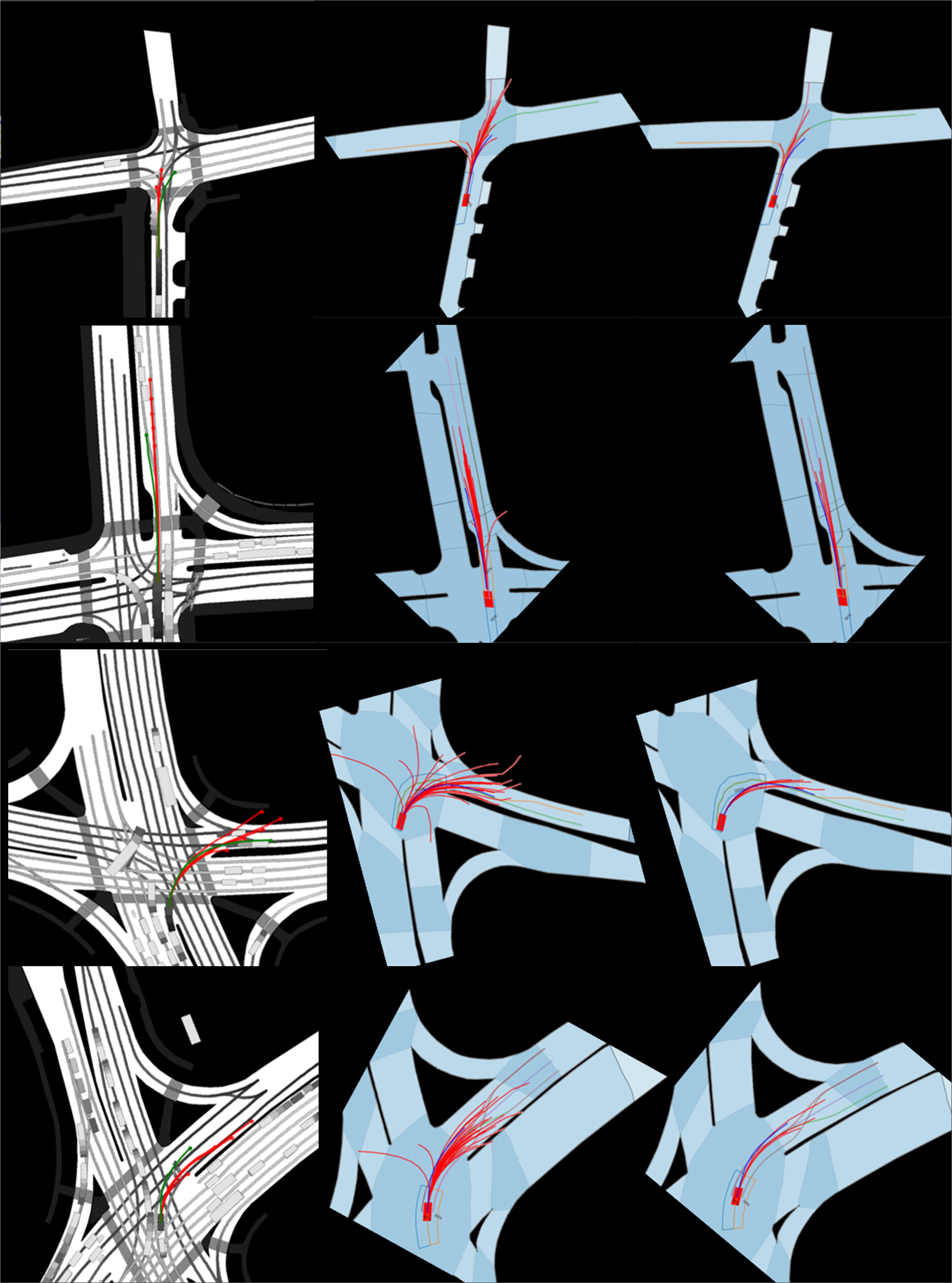
Figure 6: Illustration of the qualitative result. Column 1 is SemanticFormer 5 predictions. Column 2 is SemanticFormer 25 predictions. Column 3 is the Results of SemanticFormerR, predictions refinement

V CONCLUSIONS

This paper proposes a novel approach to reason over a semantic traffic scene graph that leverages past trajectories and an HD map as input and outputs a set of multimodal predicted trajectories. A scene graph encoder module aims to capture the interactions in a traffic scene from four aspects, agent-agent interaction, agent-map interaction, map-map interaction, and meta-paths interaction. Further, the refinement module considers the typical speed profiles and anchor paths for the refinement of trajectory candidates

Our approach achieves excellent performance which is on par with the contemporary state-of-the-art models, and several ablation studies demonstrating superior generalized performance. Moreover, extensive ablation and sensitivity studies also point out the limitations of current heterogeneous graph operators when applied to complex knowledge graphs. Future work will focus on a more complete knowledge graph if more information is included like traffic rules, traffic signs, and other common sense.

References

- [1] H. Cui, V. Radosavljevic, F.-C. Chou, T.-H. Lin, T. Nguyen, T.-K. Huang, J. G. Schneider, and N. Djuric, “Multimodal trajectory predictions for autonomous driving using deep convolutional networks,” 2019 International Conference on Robotics and Automation (ICRA), pp. 2090–2096, 2018.
- [2] T. Phan-Minh, E. C. Grigore, F. A. Boulton, O. Beijbom, and E. M. Wolff, “Covernet: Multimodal behavior prediction using trajectory sets,” 2020 IEEE/CVF Conference on Computer Vision and Pattern Recognition (CVPR), pp. 14 062–14 071, 2019.
- [3] J. Li, F. Yang, M. Tomizuka, and C. Choi, “Evolvegraph: Multi-agent trajectory prediction with dynamic relational reasoning,” arXiv: Computer Vision and Pattern Recognition, 2020.
- [4] J. Gao, C. Sun, H. Zhao, Y. Shen, D. Anguelov, C. Li, and C. Schmid, “Vectornet: Encoding hd maps and agent dynamics from vectorized representation,” 2020 IEEE/CVF Conference on Computer Vision and Pattern Recognition (CVPR), pp. 11 522–11 530, 2020.
- [5] L. Mlodzian, Z. Sun, H. Berkemeyer, S. Monka, Z. Wang, S. Dietze, L. Halilaj, and J. Luettin, “nuscenes knowledge graph - A comprehensive semantic representation of traffic scenes for trajectory prediction,” in IEEE/CVF International Conference on Computer Vision, ICCV 2023 - Workshops. IEEE, 2023, pp. 42–52.
- [6] H. Caesar, V. Bankiti, A. H. Lang, S. Vora, V. E. Liong, Q. Xu, A. Krishnan, Y. Pan, G. Baldan, and O. Beijbom, “nuScenes: A multimodal dataset for autonomous driving,” in Proceedings of the IEEE/CVF conference on computer vision and pattern recognition, 2020, pp. 11 621–11 631.
- [7] H. Berkemeyer, R. Franceschini, T. Tran, L. Che, and G. Pipa, “Feasible and adaptive multimodal trajectory prediction with semantic maneuver fusion,” 2021 IEEE International Conference on Robotics and Automation (ICRA), pp. 8530–8536, 2021.
- [8] T. Gilles, S. Sabatini, D. Tsishkou, B. Stanciulescu, and F. Moutarde, “Home: Heatmap output for future motion estimation,” in International Conference on Intelligent Transportation Systems, 2021.
- [9] T. Gilles, S. Sabatini, D. V. Tsishkou, B. Stanciulescu, and F. Moutarde, “Gohome: Graph-oriented heatmap output for future motion estimation,” 2022 International Conference on Robotics and Automation (ICRA), pp. 9107–9114, 2021.
- [10] T. Gilles, S. Sabatini, D. Tsishkou, B. Stanciulescu, and F. Moutarde, “THOMAS: trajectory heatmap output with learned multi-agent sampling,” 2022.
- [11] M. Liang, B. Yang, R. Hu, Y. Chen, R. Liao, S. Feng, and R. Urtasun, “Learning lane graph representations for motion forecasting,” 2020.
- [12] S. Casas, C. Gulino, R. Liao, and R. Urtasun, “Spagnn: Spatially-aware graph neural networks for relational behavior forecasting from sensor data,” 2020 IEEE International Conference on Robotics and Automation (ICRA), pp. 9491–9497, 2019.
- [13] B. Varadarajan, A. S. Hefny, A. Srivastava, K. S. Refaat, N. Nayakanti, A. Cornman, K. M. Chen, B. Douillard, C. P. Lam, D. Anguelov, and B. Sapp, “Multipath++: Efficient information fusion and trajectory aggregation for behavior prediction,” 2022 International Conference on Robotics and Automation (ICRA), pp. 7814–7821, 2021.
- [14] S. Konev, “Mpa: Multipath++ based architecture for motion prediction,” ArXiv, vol. abs/2206.10041, 2022.
- [15] D. Grimm, P. Schörner, M. Dressler, and J. M. Zöllner, “Holistic graph-based motion prediction,” ArXiv, vol. abs/2301.13545, 2023.
- [16] M. Liu, H. Cheng, L. Chen, H. Broszio, J. Li, R. Zhao, M. Sester, and M. Y. Yang, “Laformer: Trajectory prediction for autonomous driving with lane-aware scene constraints,” ArXiv, vol. abs/2302.13933, 2023.
- [17] H. Zhao, J. Gao, T. Lan, C. Sun, B. Sapp, B. Varadarajan, Y. Shen, Y. Shen, Y. Chai, C. Schmid, C. Li, and D. Anguelov, “Tnt: Target-driven trajectory prediction,” in Conference on Robot Learning, 2020.
- [18] X. Mo, Z. Huang, Y. Xing, and C. Lv, “Multi-agent trajectory prediction with heterogeneous edge-enhanced graph attention network,” IEEE Transactions on Intelligent Transportation Systems, vol. 23, pp. 9554–9567, 2022.
- [19] X. Jia, P. Wu, L. Chen, H. Li, Y. S. Liu, and J. Yan, “Hdgt: Heterogeneous driving graph transformer for multi-agent trajectory prediction via scene encoding,” ArXiv, vol. abs/2205.09753, 2022.
- [20] T. Monninger, J. Schmidt, J. Rupprecht, D. Raba, J. Jordan, D. Frank, S. Staab, and K. Dietmayer, “SCENE: Reasoning about traffic scenes using heterogeneous graph neural networks,” IEEE Robotics and Automation Letters, vol. 8, no. 3, pp. 1531–1538, mar 2023.
- [21] S. Wonsak, M. Al-Rifai, M. Nolting, and W. Nejdl, “Multi-modal motion prediction with graphormers,” in 2022 IEEE 25th International Conference on Intelligent Transportation Systems (ITSC) October 8-12, 2022, Macau, China. IEEE, 2022.
- [22] M. Zipfl, F. Hertlein, A. Rettinger, S. Thoma, L. Halilaj, J. Luettin, S. Schmid, and C. A. Henson, “Relation-based motion prediction using traffic scene graphs,” 2022 IEEE 25th International Conference on Intelligent Transportation Systems (ITSC), pp. 825–831, 2022.
- [23] A. Vaswani, N. M. Shazeer, N. Parmar, J. Uszkoreit, L. Jones, A. N. Gomez, L. Kaiser, and I. Polosukhin, “Attention is all you need,” in Neural Information Processing Systems, 2017.
- [24] Y. Tang and R. Salakhutdinov, “Multiple futures prediction,” in Neural Information Processing Systems, 2019.
- [25] K. Messaoud, I. Yahiaoui, and F. N. Anne Verroust-Blondet, “Attention based vehicle trajectory prediction.” IEEE, 2020.
- [26] S. Park, G. Lee, M. Bhat, J. Seo, M. Kang, J. M. Francis, A. R. Jadhav, P. P. Liang, and L.-P. Morency, “Diverse and admissible trajectory forecasting through multimodal context understanding,” in European Conference on Computer Vision, 2020.
- [27] Y. Yuan, X. Weng, Y. Ou, and K. Kitani, “Agentformer: Agent-aware transformers for socio-temporal multi-agent forecasting,” 2021 IEEE/CVF International Conference on Computer Vision (ICCV), pp. 9793–9803, 2021.
- [28] R. Girgis, F. Golemo, F. Codevilla, M. Weiss, J. A. D’Souza, S. E. Kahou, F. Heide, and C. J. Pal, “Latent variable sequential set transformers for joint multi-agent motion prediction,” in International Conference on Learning Representations, 2021.
- [29] S. Khandelwal, W. Qi, J. Singh, U. of British, C. Carnegie, M. University, and A. AI, “What-if motion prediction for autonomous driving,” in IEEE/RJS International Conference on Intelligent RObots and Systems, 2022.
- [30] Y. Liu, J. Zhang, L. Fang, Q. Jiang, and B. Zhou, “Multimodal motion prediction with stacked transformers,” 2021, pp. 7573–7582.
- [31] Z. Huang, X. Mo, and C. Lv, “Multi-modal motion prediction with transformer-based neural network for autonomous driving,” 2022 International Conference on Robotics and Automation (ICRA), pp. 2605–2611, 2021.
- [32] J. Ngiam, V. Vasudevan, B. Caine, Z. Zhang, H.-T. L. Chiang, J. Ling, R. Roelofs, A. Bewley, C. Liu, A. Venugopal, D. J. Weiss, B. Sapp, Z. Chen, and J. Shlens, “Scene transformer: A unified architecture for predicting future trajectories of multiple agents,” in International Conference on Learning Representations, 2022.
- [33] N. Nayakanti, R. Al-Rfou, A. Zhou, K. Goel, K. S. Refaat, and B. Sapp, “Wayformer: Motion forecasting via simple & efficient attention networks,” 2023 IEEE International Conference on Robotics and Automation (ICRA), pp. 2980–2987, 2022.
- [34] S. Shi, L. Jiang, D. Dai, and B. Schiele, “Motion transformer with global intention localization and local movement refinement,” ArXiv, vol. abs/2209.13508, 2022.
- [35] J. P. Mercat, T. Gilles, N. E. Zoghby, G. Sandou, D. Beauvois, and G. P. Gil, “Multi-head attention for multi-modal joint vehicle motion forecasting,” 2020 IEEE International Conference on Robotics and Automation (ICRA), pp. 9638–9644, 2019.
- [36] Z. Zhou, L. Ye, J. Wang, K. Wu, and K. Lu, “Hivt: Hierarchical vector transformer for multi-agent motion prediction,” 2022 IEEE/CVF Conference on Computer Vision and Pattern Recognition (CVPR), pp. 8813–8823, 2022.
- [37] S. Casas, C. Gulino, S. Suo, K. Luo, R. Liao, and R. Urtasun, “Implicit latent variable model for scene-consistent motion forecasting,” in European Conference on Computer Vision, 2020.
- [38] S. V. Albrecht, C. Brewitt, J. Wilhelm, B. Gyevnar, F. Eiras, M. S. Dobre, and S. Ramamoorthy, “Interpretable goal-based prediction and planning for autonomous driving,” 2021 IEEE International Conference on Robotics and Automation (ICRA), pp. 1043–1049, 2020.
- [39] J. Gu, C. Sun, and H. Zhao, “Densetnt: End-to-end trajectory prediction from dense goal sets,” 2021 IEEE/CVF International Conference on Computer Vision (ICCV), pp. 15 283–15 292, 2021.
- [40] N. Deo and M. M. Trivedi, “Trajectory forecasts in unknown environments conditioned on grid-based plans,” ArXiv, vol. abs/2001.00735, 2020.
- [41] Y. Chai, B. Sapp, M. Bansal, and D. Anguelov, “Multipath: Multiple probabilistic anchor trajectory hypotheses for behavior prediction,” in Conference on Robot Learning, 2019.
- [42] E. Amirloo, A. Rasouli, P. Lakner, M. Rohani, and J. Luo, “Latentformer: Multi-agent transformer-based interaction modeling and trajectory prediction,” ArXiv, vol. abs/2203.01880, 2022.
- [43] X. Wang, H. Ji, C. Shi, B. Wang, Y. Ye, P. Cui, and P. S. Yu, “Heterogeneous graph attention network,” in The world wide web conference, 2019, pp. 2022–2032.
- [44] A. Naumann, F. Hertlein, D. Grimm, M. Zipfl, S. Thoma, A. Rettinger, L. Halilaj, J. Luettin, S. Schmid, and H. Caesar, “Lanelet2 for nuscenes: Enabling spatial semantic relationships and diverse map-based anchor paths,” in Proceedings of the IEEE/CVF Conference on Computer Vision and Pattern Recognition, 2023, pp. 3247–3256.
- [45] T. Salzmann, B. Ivanovic, P. Chakravarty, and M. Pavone, “Trajectron++: Dynamically-feasible trajectory forecasting with heterogeneous data,” in Computer Vision–ECCV 2020: 16th European Conference, Glasgow, UK, August 23–28, 2020, Proceedings, Part XVIII 16. Springer, 2020, pp. 683–700.
- [46] B. Kim, S. H. Park, S. Lee, E. Khoshimjonov, D. Kum, J. Kim, J. S. Kim, and J. W. Choi, “Lapred: Lane-aware prediction of multi-modal future trajectories of dynamic agents,” in Proceedings of the IEEE/CVF Conference on Computer Vision and Pattern Recognition (CVPR), June 2021, pp. 14 636–14 645.
- [47] N. Deo, E. M. Wolff, and O. Beijbom, “Multimodal trajectory prediction conditioned on lane-graph traversals,” in Conference on Robot Learning, 2021.
- [48] J. Chen, Z. Wang, J. Wang, and B. Cai, “Q-eanet: Implicit social modeling for trajectory prediction via experience-anchored queries,” IET Intelligent Transport Systems, 2023.
- [49] D.-H. Park, H. Ryu, Y. Yang, J. Cho, J. Kim, and K.-J. Yoon, “Leveraging future relationship reasoning for vehicle trajectory prediction,” ArXiv, vol. abs/2305.14715, 2023.