Nonlocal electrodynamics and the penetration depth of superconducting Sr₂RuO₄

Abstract

The thermal quasiparticles in a clean type-II superconductor with line nodes give rise to a quadratic low-temperature change of the penetration depth, $\Delta\lambda\sim T^{2}$, as first shown by Kosztin and Leggett [I. Kosztin and A. J. Leggett, Phys. Rev. Lett. 79, 135 (1997)]. Here, we generalize this result to multiple nodes and compare it to numerically exact evaluations of the temperature-dependent penetration depth in Sr₂RuO₄ using a high-precision tight-binding model. We compare the calculations to recent penetration depth measurements in high purity single crystals of Sr₂RuO₄ [J. F. Landaeta et al., arXiv:2312.05129]. When assuming the order parameter to have $\mathrm{B}_{1\mathrm{g}}$ symmetry, we find that both a simple $d_{x^{2}-y^{2}}$-wave and complicated gap structures with contributions from higher harmonics and accidental nodes can accommodate the experimental data.

I Introduction

Obtaining a detailed understanding of the superconducting state in Sr₂RuO₄ remains an important outstanding problem [1, 2, 3]. Experimentally, the quest is complicated due to challenging material properties of Sr₂RuO₄ and the low energy scale of the superconducting phase. Theoretically, Sr₂RuO₄ provides an important testbed for modeling of unconventional superconductivity. More specifically, the well-characterized electronic properties of the normal state offers a rather unique opportunity to test various electronic fluctuation-based mechanisms for pairing against detailed measurements of the superconducting gap structure [4, 5, 6, 7, 8, 9, 10, 11, 12, 13, 14, 15, 16, 17, 18, 19, 20, 21, 22, 23].

The magnetic penetration depth, $\lambda$, can elucidate nodal features of the gap, as revealed through its dependency on temperature and disorder [24, 25, 26, 27]. Fully-gapped superconductors exhibit exponential temperature dependence at low temperatures, whereas nodal gaps display power law dependence. In Sr₂RuO₄, measurements of the change in penetration depth, $\Delta\lambda(T)$, via a tunnel diode oscillator method yielded $\Delta\lambda(T)\sim T^{2}$, signalling the existence of nodal quasiparticle excitations [28]. Renewed measurements of $\Delta\lambda(T)$ in Sr₂RuO₄ high-purity spherical single crystals by applying scanning SQUID microscopy [29] and ac-susceptibility measurements [30] have confirmed this behavior and highlighted the importance of nonlocal Meissner screening. Indeed, as initially demonstrated by Kosztin and Leggett, nonlocal effects may change the low temperature dependence of the penetration depth, e.g., from linear to quadratic in $d_{x^{2}-y^{2}}$-wave superconductors, such as the cuprates [31, 32]. The relevance of nonlocal effects in an extended temperature regime is controlled by the zero-temperature Ginzburg–Landau parameter, i.e., the ratio of the penetration depth to the coherence length. In Sr₂RuO₄ this ratio is $\kappa_{0}\approx 1.92$ [30], placing this material unusually close to the Pippard limit compared to most clean, unconventional superconductors. Finally, we note that the penetration depth was also recently extracted from SQUID susceptometry in thin Sr₂RuO₄ films, again yielding $\Delta\lambda(T)\sim T^{2}$ behavior at low $T$ [33]. There, however, the origin of the $T^{2}$ dependence was interpreted in terms of disorder scattering similar to disordered $d_{x^{2}-y^{2}}$-wave superconductors [34].

Here we perform a theoretical study of the nonlocal electrodynamics specifically relevant for nodal multi-band superconductors. We perform both an exact numerical evaluation of $\Delta\lambda(T)$ and compare this to a generalized nonlocal node-expansion similar to the method by Kosztin and Leggett [31], but for cases with several distinct nodes in the Brillouin zone, possibly distributed across multiple bands. To examine whether the superconducting order parameter can be constrained from low-temperature penetration depth data, we apply the developed theory to Sr₂RuO₄. To minimize uncertainties in the description of the normal state, we use a tight-binding model that fits both the experimental Fermi surface and Fermi velocity with unprecedented accuracy. We explore two nodal superconducting gaps with B_1g symmetry, relevant for Sr₂RuO₄, and compare the node-expansion with the numerically exact result. The analytical analysis shows that the low-temperature slope of $\Delta\lambda(T)$ as a function of $(T/T_{c})^{2}$ is controlled by the sum of reciprocal gap velocities at the order parameter nodes and the corresponding Fermi velocities, the latter are experimentally known from ARPES measurements [35]. The analysis implies that the penetration depth in isolation is not sensitive to the details of the gap structure since the effect of having one shallow node can be compensated for by instead having two steeper nodes etc. The numerical simulations reveal that both gap structures explored can explain the presently available experimental data for the penetration depth of Sr₂RuO₄.

II Penetration depth

Kosztin and Leggett showed that thermal quasiparticles in a clean, type-II, nodal $d$-wave superconductor are responsible for the behavior $\Delta\lambda\sim T^{2}$ for $T<T^{\ast}$ with $T^{\ast}=\Delta_{0}/\kappa_{0}$, where $\Delta_{0}$ is gap scale and $\kappa_{0}=\lambda_{0}/\xi_{0}$ ($\lambda_{0}$ and $\xi_{0}$ is the penetration depth and the coherence length, respectively) the zero-temperature Ginzburg–Landau parameter [31]. The key ingredient here are the nonlocal effects (diverging coherence length) experienced by the Cooper pairs formed by momenta near the nodal points, see Fig. 1. This causes the penetration depth increase to acquire an additional factor of $T$ (on top of the $2k_{B}T\ln{2}/\Delta_{0}$ local contribution) coming from the inverse thermal de Broglie wavelength at low temperatures.

In Sr₂RuO₄ the behaviour $\Delta\lambda\sim T^{2}$ is observed in a dominant fraction of the temperature window below $T_{c}\approx 1.5$ K, which is consistent with this material being a marginal type-II superconductor with $\kappa_{0}\approx 1.92>1/\sqrt{2}$ [30, 28, 29] and $\Delta_{0}\approx 0.35$ meV [36, 29]. Interestingly, Sr₂RuO₄ is closer to the Pippard limit than most unconventional type-II superconductors. Owing to its clean crystals, this points to the importance of nonlocal electrodynamics to understand its superconducting state, possibly also its response to a weak magnetic field as posed by muons [37].

II.1 Nonlocal electrodynamics

In a weak magnetic field, linear response theory for the Meissner state dictates the decay of the magnetic field into the superconductor, as per $j(y)=-\int\mathrm{d}y^{\prime}~{}K(y-y^{\prime})A(y^{\prime})$. Here, $j$ is the screening supercurrent density (along $\hat{x}$) with the boundary between vacuum and the superconductor at $y=0$, and $A$ is the magnetic vector potential. The geometry is shown in Fig. 1.

Figure 1: Geometry and magnetic field (along $\hat{z}$) penetration into the Meissner state of the superconductor located in the half-plane $y>0$. The magnetic penetration depth is denoted by $\lambda$. Inset: reciprocal space of a tetragonal crystal with the Fermi surface of Sr₂RuO₄ and the nodal line (dashed) of the B_1g irreducible representation indicated. Close to the nodal point(s), the Cooper pairs are characterized by a long coherence length and hence acquire nonlocal contributions in their electromagnetic response.

In dimensionless units, $\tilde{K}=(4\pi\lambda_{0}^{2}/c)K$, and with the kernel difference defined as $\delta\tilde{K}(\tilde{q};T)\equiv\tilde{K}(\tilde{q};T)-\tilde{K}(\tilde{q};0)$, the penetration depth change can be expressed as

$$\frac{\Delta\lambda(T)}{\lambda_{0}}=\frac{2}{\pi}\int_{0}^{\infty}\frac{-\delta\tilde{K}(\tilde{q};T)~{}\mathrm{d}\tilde{q}}{\big{(}\tilde{q}^{2}+\tilde{K}(\tilde{q};0)\big{)}\big{(}\tilde{q}^{2}+1+\delta\tilde{K}(\tilde{q};T)\big{)}},$$ (1)

where $\tilde{q}=q\lambda_{0}$. We emphasize that this is an exact expression that includes a correction responsible for an upturn in $\Delta\lambda$ at higher $T$ as compared to Ref. 31. The dimensionless kernel can be computed by means of standard Green’s function methods, assuming linear response in the Meissner state and solving the relevant Maxwell equation in the superconductor [38]. In the Matsubara representation the kernel can be expressed as [38, 31]

$$\tilde{K}(\tilde{q};T)=2\pi k_{B}T\sum_{n=-\infty}^{\infty}\left\langle\frac{\hat{p}_{\parallel}^{2}\Delta_{\boldsymbol{p}}^{2}}{\sqrt{\omega_{n}^{2}+\Delta_{\boldsymbol{p}}^{2}}(\omega_{n}^{2}+\Delta_{\boldsymbol{p}}^{2}+\alpha^{2})}\right\rangle_{\mathrm{FS}},$$ (2)

where the fermionic Matsubara frequencies are given by $\omega_{n}=\pi k_{B}T(2n+1)$, $\hat{p}_{\parallel}=\cos(\theta)$ is the Fermi surface momentum projected onto the boundary ($\theta$ is the polar angle of $\boldsymbol{p}$), and the parameter $\alpha=\pi\Delta_{0}\tilde{q}\sin(\theta)/(2\kappa_{0})$ is the projected magnetic field penetration and is responsible for the nonlocal effects. Here, we employed the BCS expression for the coherence length, such that $\lambda_{0}=v_{F}\kappa_{0}/(\pi\Delta_{0})$. Finally, $\Delta_{\boldsymbol{p}}$ is the (temperature-dependent) order parameter, and the (dimensionless) Fermi surface average is evaluated as $\langle h\rangle_{\mathrm{FS}}\equiv(\bar{v}_{F}/\lvert S_{F}\rvert)\int_{S_{F}}\mathrm{d}\hat{\boldsymbol{k}}~{}h(\hat{\boldsymbol{k}})/v_{F}(\hat{\boldsymbol{k}})$ where $v_{F}(\hat{\boldsymbol{k}})$ is the Fermi velocity and $\lvert S_{F}\rvert$ the Fermi surface area. It can be noted that the zero-temperature kernel, $\tilde{K}(\tilde{q};0)$, has a simple closed-form expression, as stated in Appendix A.

In practice, realistic modelling of $\Delta\lambda/\lambda_{0}$ in the entire temperature window below $T_{c}$ is achieved by feeding in a high-precision multiband tight-binding model, as well as experimental values for $\kappa_{0}$, $\Delta_{0}$, and $T_{c}$. Since the sum in Eq. (2) converges rapidly, one can in practice calculate the Fermi surface average for each frequency and truncate the Matsubara series at some $n\gg\frac{\Delta_{0}}{2\pi k_{B}T}$ for any non-zero $T$ . If one models the $T$ dependence of the gap by the interpolation formula $\tanh{(1.74\sqrt{T/T_{c}-1})}$, the only remaining degrees of freedom lie in the momentum-dependent gap structure.

II.2 The node approximation

Building on the Kosztin–Leggett philosophy at the lowest $T$, useful insights can be harvested by first rewriting Eq. (2) using contour integration techniques, and then linearizing the gap around its nodes, $\Delta_{\boldsymbol{p}}\approx\sum_{j}v_{\Delta,j}(\theta-\theta_{j})$, where the thermally active quasiparticles are situated at the lowest $T$. We will henceforth refer to $v_{\Delta,j}$ as the “gap velocity” at node $j$. The dimensionless kernel difference, with the intermediate steps shown in Appendix A, can in this case be recast as

$$-\delta\tilde{K}(\tilde{q};T) \approx k_{B}T\frac{2\pi\ln{2}}{\lvert S_{F}\rvert}\sum_{j}\frac{2\hat{p}_{\parallel,j}^{2}\bar{v}_{F}}{v_{F,j}v_{\Delta,j}}\Big{\lvert}\frac{\partial\boldsymbol{k}_{F}}{\partial\theta}\Big{\rvert}_{j}$$ (3)

$$\times\left[1-\frac{1}{\ln{2}}\int_{0}^{\alpha_{j}/T}\mathrm{d}x~{}\tilde{f}(x)\sqrt{1-\left(xT/\alpha_{j}\right)^{2}}\right],$$

where $\tilde{f}(x)=(1+\exp(x))^{-1}$ is the Fermi function and where the sum runs over distinct nodes in the Brillouin zone (possibly distributed across multiple bands). The symbols are otherwise explained earlier. This result is a multiband generalization of the node approximation proposed by Kosztin and Leggett. To make evaluation fast we further approximate $\tilde{K}(\tilde{q};0)\approx 1=\tilde{K}(0;0)$ in Eq. (1) when evaluating the penetration depth from the node approximation in the next section.

To validate the above expression, we benchmark it in the simple $d_{x^{2}-y^{2}}$-wave case ($\Delta_{\boldsymbol{p}}=\Delta_{0}\cos(2\theta)$) using a circular Fermi surface and isotropic Fermi velocity. The four distinct nodes all have $\hat{p}_{\parallel}^{2}=1/2$ and the associated gap velocities are $v_{\Delta}=2\Delta_{0}$. In this case we recover the standard result $\delta\tilde{K}(\tilde{q};T)=\delta\tilde{K}(0;T)F(\tilde{q}/t)$, where $t=T/T^{\ast}$, with $T^{\ast}=\Delta_{0}/\kappa_{0}$, and $F$ is a universal function similar to the lower line in Eq. (3), stated in Appendix A. The prefactor reduces to the well-known $-\delta\tilde{K}(0;T)=2k_{B}T\ln{2}/\Delta_{0}$, i.e., the local result [34, 32, 40]. The function $F$ ensures that below the characteristic temperature scale $T^{\ast}$, the change in the penetration depth depends quadratically on temperature, $\Delta\lambda\sim T^{2}$.

For the multinode generalization in Eq. (3) the above-mentioned factorization breaks down, and the kernel difference instead depends on all of the distinct $\tilde{q}/t_{j}$ where $t_{j}\propto\frac{\Delta_{0}}{\kappa_{0}}\sin(\theta_{j})$ for each distinct gap node $j$. Thus, each distinct gap node is associated with a characteristic temperature scale, the minimum of which dictates the regime in which $\Delta\lambda\sim T^{2}$. Some key insights are gained by the details added to Eq. (3) caused by having a non-isotropic Fermi surface and higher-harmonic gap structure, possibly with multiple distinct nodes. Equation (3) tells us that $\lim_{T\to T_{c}}\Delta\lambda(T)/(T/T_{c})^{2}$ is proportional to a weighted sum over the distinct gap nodes, where the weight contains a product of the reciprocal gap velocity and the reciprocal Fermi velocity. The primer is strain-tunable and implies an enhanced sensitivity to gap structures with nodes at strain-induced van Hove points. In the context of Sr₂RuO₄, no substantial variations in the penetration depth slope change are detected as uniaxial strain is applied [29], which argues against both B_2g ($d_{xy}$) and A_2g ($g_{xy(x^{2}-y^{2})}$) type orders, which is also consistent with elastocaloric measurements [41]. Generally, however, the dependency on the reciprocal gap velocities implies that penetration depth data alone do not impose any crisp constraints on the momentum structure of the gap, since the effect of having one shallow node can be compensated for by having two steeper nodes.

There are at least two reasons why there are few candidate materials for observing $\Delta\lambda\sim T^{2}$ from the above mechanism. First, disorder is known to cause a saturation of $\Delta\lambda$ below a characteristic temperature set by the scattering rate [34], which will effectively blur the observation of a quadratic temperature dependence. Second, the most well-characterized $d$-wave superconductors are strong type-II, $\kappa_{0}\gg 1$, suppressing $T^{\ast}$ to a tiny fraction of the gap. In both of these respects Sr₂RuO₄ poses as a counterexample, since it has accumulated strong evidence of being both nodal [42, 43], marginal type-II [30], and is known to produce clean and disorder-sensitive crystals [44]. Other candidate superconductors possibly relevant to a low-$T$ penetration depth of $\Delta\lambda\sim T^{2}$ caused by nonlocal electrodynamics include cuprates [31], KFe₂As₂ [45], and the heavy-fermion material CeCoIn₅ [46, 24]. Below we focus on the case of Sr₂RuO₄.

III The case of Strontium Ruthenate

III.1 Tight-binding model

We depart from a standard three-band tight-binding model ansatz for Sr₂RuO₄,

$$H_{0}=\sum_{\boldsymbol{k},\sigma}\vec{\psi}^{\dagger}_{\sigma}(\boldsymbol{k})\pazocal{H}_{\sigma}(\boldsymbol{k})\vec{\psi}_{\sigma}(\boldsymbol{k}),$$ (4)

where $\vec{\psi}_{s}(\boldsymbol{k})=[c_{xz,s}(\boldsymbol{k}),\hskip 2.84526ptc_{yz,s}(\boldsymbol{k}),\hskip 2.84526ptc_{xy,-s}(\boldsymbol{k})]^{\mathrm{T}}$, $\sigma=\pm$ denotes spin, and $a\in\{xz,yz,xy\}$ labels the Ru $d$-orbitals (the $t_{2\mathrm{g}}$ triplet), which are the only relevant orbitals close to the Fermi energy [47].

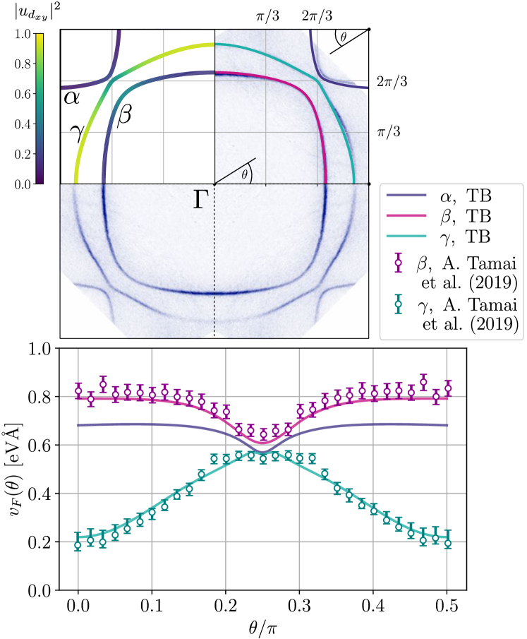
Figure 2: Fermi surface and Fermi velocities of Sr₂RuO₄. Model ($k_{z}=0$): solid lines (labelled “TB”) show the model Fermi surface (top panel) and the Fermi velocities (bottom panel). The second quadrant in the top panel shows the Ru $d_{xy}$ orbital content of the bands. The average model Fermi velocity is $\bar{v}_{F}=0.498$ eVÅ. Data: high-resolution ARPES Fermi surface (dark blue, top panel) and the Fermi velocities (circles with error bars, bottom panel) extracted from Ref. 35.

The form of $\pazocal{H}_{\sigma}$ is

$$\pazocal{H}_{\sigma}(\boldsymbol{k})=\begin{pmatrix}\xi_{xz}(\boldsymbol{k})&\xi_{xz,yz}(\boldsymbol{k})-i\sigma\eta&i\eta\\ \xi_{xz,yz}(\boldsymbol{k})+i\sigma\eta&\xi_{yz}(\boldsymbol{k})&-\sigma\eta\\ -i\eta&-\sigma\eta&\xi_{xy}(\boldsymbol{k})\end{pmatrix},$$ (5)

where spin-orbit coupling is parametrized by $\eta$ and originates from the (dominant) onsite term $2\eta\sum_{i}\vec{L}_{i}\cdot\vec{S}_{i}$ as projected onto the $t_{2g}$ Ru triplet. Explicit forms of the inter- and intraband energies are listed in Appendix B.

To obtain a quantitatively accurate parametrization, we consider as a starting point the tight-binding parameters from Ref. 23 as derived from relativistic DFT calculations. While these parameters provide a realistic energy scale and Fermi surface, they still do not quantitatively match the Fermi velocities as extracted from high-resolution ARPES measurements for bands $\beta$ and $\gamma$ in Ref. 35. To correct for this discrepancy, which is also present in another tight-binding model widely employed in the literature [48], we manually tune tight-binding parameters until a reasonable match with both the experimental Fermi surface and Fermi velocity $v_{F}$ is obtained. The result is shown in Fig. 2. The effective model, with the set of parameters listed in Appendix B, provides a high-precision effective normal state description of Sr₂RuO₄. We stress that a model that is qualitatively and quantitatively accurate in the above respect could be crucial to accurately perform calculations sensitive to $v_{F}$.

III.2 Numerical evaluation of the penetration depth

Equipped with an accurate description of the normal state, we now turn to the evaluation of the penetration depth difference, $\Delta\lambda(T)/\lambda_{0}$, for some illustrative order parameters.

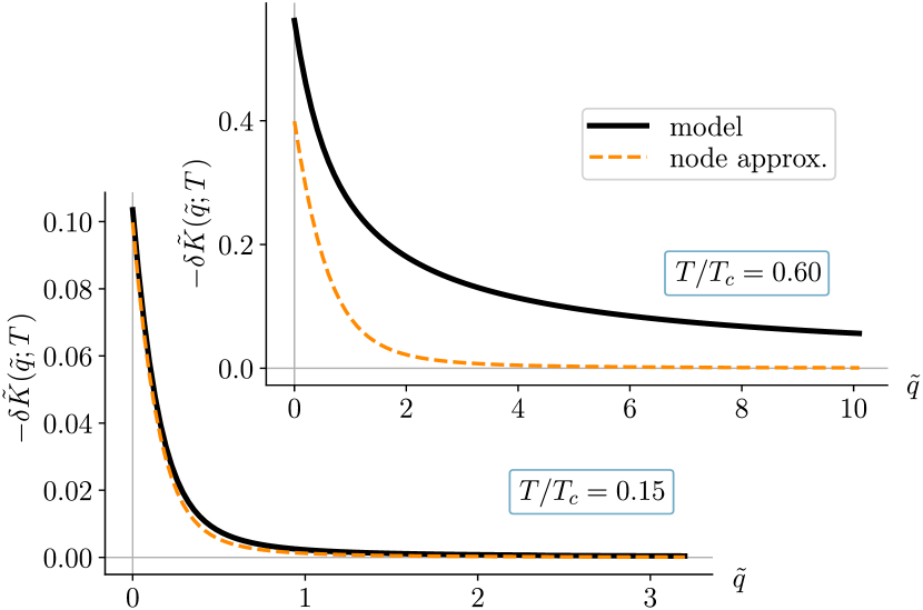
Figure 3: Dimensionless kernel differences, $-\delta\tilde{K}(\tilde{q};T)$, calculated at $T=0.15T_{c}$ and $T=0.6T_{c}$ for both the node approximation of Eq. (3) (“node approx.”) and in the Matsubara representation (“model”). We use the three-band tight-binding model of Sec. III.1 and order parameters of Fig. 4(a). Due to the curvature of $\Delta(\theta)$, the node approximation overestimates the gap and underestimates the penetration depth at higher temperatures.

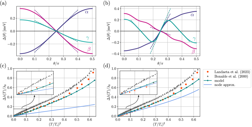
Figure 4: Representative B_1g order parameters [(a) and (b)], and associated penetration depths [(c) associated with (a), and (d) associated with (b)] using both the node approximation (“node approx.”) and the Mastubara representation (“model”) to calculate the kernel. We use the three-band tight-binding model of Sec. III.1. Experimental data points from Refs. 28, 30 are plotted as gray triangles and orange disks for comparison. In (a) and (b) linearizations around the gap nodes are shown with dashed lines.

First, we calculate the kernel difference $-\delta\tilde{K}(\tilde{q};T)$ at two temperatures using both the node approximation of Eq. (3) and the full Matsubara sum of Eq. (2). For illustration we employ the simplest gap structure consistent with B_1g symmetry, i.e., $\Delta_{0}\cos(2\theta)$ on all bands with $\Delta_{0}=0.35$ meV on bands $\alpha$ and $\beta$, and half the magnitude on band $\gamma$. These values are motivated by STM experiments [36, 29], and the gap magnitude on $\gamma$ was reduced to match the experimental penetration depth slope at low $T$. We otherwise fixed $\kappa_{0}=1.92$ and $T_{c}=1.5$ K, in agreement with experiments [30]. The resulting kernel differences are shown in Fig. 3, and the order parameter and penetration depth are shown in Fig. 4(a) and (c).

Comparing the penetration depth calculations with the experimental data reveals that the temperature window in which the node approximation matches with the realistic modelling is roughly $T/T_{c}\lesssim 0.2$. The primary reason for this is the overestimated slope of $\lvert\Delta(\theta)\rvert$ when linearizing the gap, causing the node approximation to, in this case, monotonically underestimate the penetration depth. Additionally, the $T$ dependence of the gap and the correction posed by the denominator of Eq. (1) both contribute with an upturn in $\Delta\lambda(T)$ close to the transition temperature $T_{c}$, approximately consistent with the experimental data. The realistic modelling shows that a simple $d_{x^{2}-y^{2}}$-wave gap is sufficient to explain the experimental data, albeit with a slight discrepancy at the highest $T$.

In Fig. 4(b) and (d) we show the results of calculating the penetration depth for a more involved order parameter, still within the B_1g irreducible representation, but with an angular dependence inspired by weak-coupling and RPA spin-fluctuation calculations [6, 11, 49, 50]. In this case, the node approximation performs better when comparing to the realistic modelling. Since the order parameter is more involved by having contributions from multiple harmonics, the error introduced by linearizing the gap is non-monotonic, i.e., the gap is both over- and underestimated on the various bands. As the realistic modelling shows, an equally convincing $T$-dependent penetration depth is obtained for this order parameter. Therefore, not surprisingly, the change in the penetration depth is not capable of resolving subtle differences in the the nodal structure of the order parameter. As the nodal expansion reveals, the slope of $\Delta\lambda(T)$ as a function of $(T/T_{c})^{2}$ at the lowest temperatures is a weighted sum of reciprocal gap velocities at the nodes, so the increase in slope gained by an additional node can be compensated for by increasing the gap velocity of one or more nodes.

IV Conclusions

In summary, we have calculated the temperature-dependent change of the penetration depth $\Delta\lambda$ including nonlocal effects from line nodes. We have provided both a multi-band multi-node generalization of the Kosztin-Leggett result [31], and demonstrated a straightforward numerical procedure to evaluate $\Delta\lambda$ numerically exact, given a multi-band tight-binding description. Focusing on the case of Sr₂RuO₄, posing as a prime candidate material owing to its clean crystals and evidence of nodal order, we investigated two $d$-wave gap structures with different nodal properties. The analysis reveals that the low-temperature penetration depth is sensitive to the sum of reciprocal gap velocities at the nodes, and that both orders investigated have nodal properties compatible with the presently available data.

V Acknowledgements

We acknowledge useful discussions with C. Hicks. H.S.R. was supported by research Grant No. 40509 from VILLUM FONDEN. A.K. acknowledges support by the Danish National Committee for Research Infrastructure (NUFI) through the ESS-Lighthouse Q-MAT.

Appendix A Generalized Kosztin–Leggett theory

Here, we re-derive and generalize the central result of Kosztin and Leggett [31] for the penetration depth of a nodal type-II superconductor.

In a weak magnetic field, the Meissner state of a superconductor responds linearly to the perturbation,

$$j(y)=-\int\mathrm{d}y^{\prime}K(y-y^{\prime})A(y^{\prime}).$$ (6)

Here, $j$ is the screening supercurrent density (pointing along $\hat{x}$, $y=0$ is the position of the superconductor boundary), $K$ is the electromagnetic response kernel, and $A$ is the magnetic vector potential. With a specular boundary, the magnetic penetration depth is given by

$$\frac{\lambda(T)}{\lambda_{0}}=\frac{2}{\pi}\int_{0}^{\infty}\frac{\mathrm{d}\tilde{q}}{\tilde{q}^{2}+\tilde{K}(\tilde{q};T)},$$ (7)

where $\tilde{q}=\lambda_{0}q$ with $\lambda_{0}\equiv\lambda(0)$, and $\tilde{K}=(4\pi\lambda_{0}^{2}/c)K$. The dimensionless kernel satisfies $\tilde{K}(\tilde{q}\to 0;0)=1$ in the local limit. Writing $\tilde{K}(\tilde{q};T)=1+\delta\tilde{K}(\tilde{q};T)$, with $\delta\tilde{K}(\tilde{q};T)\equiv\tilde{K}(\tilde{q};T)-\tilde{K}(\tilde{q};0)$ leads to the exact expression for $\Delta\lambda(T)\equiv\lambda(T)-\lambda_{0}$ given in the main text Eq. (1). The zero temperature kernel can be evaluated analytically [31], with

$$\tilde{K}(\tilde{q};0)=1-\left\langle 2\hat{p}_{\parallel}^{2}\left[1-\frac{\mathrm{arcsinh}(\alpha/\Delta_{\boldsymbol{p}})}{\alpha/\Delta_{\boldsymbol{p}}\sqrt{1+(\alpha/\Delta_{\boldsymbol{p}})^{2}}}\right]\right\rangle_{\mathrm{FS}}.$$ (8)

Using contour integration techniques [38], the response kernel correction can be evaluated as

$$-\delta\tilde{K}(\tilde{q};T) =2\int_{0}^{\infty}\mathrm{d}\omega~{}f(\omega)$$ (9)

$$\times\left\langle 2\hat{p}_{\parallel}^{2}\mathrm{Re}\frac{\Delta_{\boldsymbol{p}}^{2}}{\sqrt{\omega^{2}-\Delta_{\boldsymbol{p}}^{2}}(\Delta_{\boldsymbol{p}}^{2}-\omega^{2}+\alpha^{2})}\right\rangle_{\mathrm{FS}},$$

where $f(\omega)=(1+\exp(\beta\omega))^{-1}$ is the Fermi function, $\Delta_{\boldsymbol{p}}$ is the order parameter, $\hat{p}_{\parallel}=\cos(\theta)$ is the projection of the Fermi surface momentum on the $\hat{x}$-axis, and $\alpha=qv_{F}\sin{\theta}/2$. Setting $\alpha=0$ reproduces the local result [34].

To evaluate the Fermi surface average, we first recast momentum sums as integrals over $(\xi,\hskip 2.84526pt\hat{\boldsymbol{k}})$, where $\hat{\boldsymbol{k}}$ lies on the Fermi surface defined by $S_{F}(\xi)\equiv\{\hat{\boldsymbol{k}}:~{}\xi_{\hat{\boldsymbol{k}}}=\xi\}$ in the following manner (introducing also the electronic cutoff $\omega_{c}$):

$$\sum_{\boldsymbol{k}:~{}\lvert\xi_{\boldsymbol{k}}\rvert<\omega_{c}}h_{\boldsymbol{k}}=\int_{-\omega_{c}}^{\omega_{c}}\mathrm{d}\xi\hskip 2.84526pt\rho_{\xi}\int_{S_{F}(\xi)}\frac{\mathrm{d}\hat{\boldsymbol{k}}}{\lvert S_{F}\rvert}\frac{\bar{v}_{F}}{v_{F}(\hat{\boldsymbol{k}})}h(\hat{\boldsymbol{k}}),$$ (10)

where the Fermi velocity, the average Fermi velocity, and the density of states are given by

$$v_{F}(\hat{\boldsymbol{k}}) =\lvert\nabla\xi_{\hat{\boldsymbol{k}}}\rvert,$$ (11)

$$\bar{v}_{F} =\Big{[}\int_{S_{F}(\xi)}\frac{\mathrm{d}\hat{\boldsymbol{k}}}{\lvert S_{F}\rvert}\frac{1}{v_{F}(\hat{\boldsymbol{k}})}\Big{]}^{-1},$$ (12)

$$\rho_{\xi} =\int_{S_{F}(\xi)}\frac{\mathrm{d}\hat{\boldsymbol{k}}}{(2\pi)^{d}}\frac{1}{v_{F}(\hat{\boldsymbol{k}})},$$ (13)

respectively, and where $\lvert S_{F}\rvert$ is the Fermi surface area. From the above we define the (dimensionless) Fermi surface average as

$$\langle A\rangle_{\mathrm{FS}}\equiv\int_{S_{F}(\xi)}\frac{\mathrm{d}\hat{\boldsymbol{k}}}{\lvert S_{F}\rvert}\frac{\bar{v}_{F}}{v_{F}(\hat{\boldsymbol{k}})}A,$$ (14)

such that $\langle 1\rangle_{\mathrm{FS}}=1$.

We next expand the order parameter around its nodes, situated at angles $\theta_{j}$, $\Delta_{\boldsymbol{p}}\approx\sum_{j}v_{\Delta,j}(\theta-\theta_{j})$, where $v_{\Delta,j}$ is the “gap velocity” of node $j$. Close to the nodes (at low temperatures), we can safely ignore the angular dependence of $\alpha$ and $\hat{p}_{\parallel}$. Since Eq. (9) picks up contributions around each node, we then get

$$-\delta\tilde{K}(\tilde{q};T) =2\int_{0}^{\infty}\mathrm{d}\omega~{}f(\omega)\left\langle 2\hat{p}_{\parallel}^{2}\mathrm{Re}\frac{\Delta_{\boldsymbol{p}}^{2}}{\sqrt{\omega^{2}-\Delta_{\boldsymbol{p}}^{2}}(\Delta_{\boldsymbol{p}}^{2}-\omega^{2}+\alpha^{2})}\right\rangle_{\mathrm{FS}}$$ (15)

$$\approx\frac{2}{\lvert S_{F}\rvert}\int_{0}^{\infty}\mathrm{d}\omega~{}f(\omega)\sum_{j}\frac{2\hat{p}_{\parallel,j}^{2}\bar{v}_{F}}{v_{F,j}v_{\Delta,j}}\Big{\lvert}\frac{\partial\boldsymbol{k}_{F}}{\partial\theta}\Big{\rvert}_{j}\int_{-\omega}^{\omega}\mathrm{Re}\frac{\mathrm{d}u~{}u^{2}}{\sqrt{\omega^{2}-u^{2}}(u^{2}-\omega^{2}+\alpha_{j}^{2})}$$

$$=\frac{2\pi}{\lvert S_{F}\rvert}\int_{0}^{\infty}\mathrm{d}\omega~{}f(\omega)\sum_{j}\frac{2\hat{p}_{\parallel,j}^{2}\bar{v}_{F}}{v_{F,j}v_{\Delta,j}}\Big{\lvert}\frac{\partial\boldsymbol{k}_{F}}{\partial\theta}\Big{\rvert}_{j}\mathrm{Re}\left[1-\sqrt{1-\omega^{2}/\alpha_{j}^{2}}\right]$$

$$=k_{B}T\frac{2\pi\ln{2}}{\lvert S_{F}\rvert}\sum_{j}\frac{2\hat{p}_{\parallel,j}^{2}\bar{v}_{F}}{v_{F,j}v_{\Delta,j}}\Big{\lvert}\frac{\partial\boldsymbol{k}_{F}}{\partial\theta}\Big{\rvert}_{j}\left[1-\frac{1}{\ln{2}}\int_{0}^{\alpha_{j}/T}\mathrm{d}x~{}\tilde{f}(x)\sqrt{1-\left(xT/\alpha_{j}\right)^{2}}\right],$$

where $\alpha_{j}=\tilde{q}v_{F,j}\sin(\theta_{j})/(2\lambda_{0})$, $\tilde{f}(x)\equiv(1+\exp(x))^{-1}$ is the Fermi function with dimensionless argument, and where the sum runs over distinct nodes in the Brillouin zone (possibly distributed across multiple bands). This result is a multiband generalization of the node approximation proposed by Kosztin and Leggett, which is a low-temperature approximation that is valid in the temperature window in which the order parameter can be reasonably approximated by a linear function of the angle deviation from the node.

To validate the generalized (multiband) expression of Eq. (15), we evaluate it for the simple $d$-wave order parameter $\Delta_{\boldsymbol{p}}=\Delta_{0}\cos(2\theta)$ and a circular Fermi surface with isotropic Fermi velocity [31]. The four distinct nodes all have $\hat{p}_{\parallel}^{2}=1/2$ and gap velocity $v_{\Delta}=2\Delta_{0}$. Further writing $\lambda_{0}=\kappa_{0}\xi_{0}$, and using the BCS expression for the coherence length, $\xi_{0}=v_{F}/(\pi\Delta_{0})$, leads to

$$-\delta\tilde{K}(\tilde{q};T) =\frac{2k_{B}T\ln{2}}{\Delta_{0}}$$ (16)

$$\times\left[1-\frac{1}{\ln{2}}\int_{0}^{\pi\frac{\sqrt{2}z}{4}}\mathrm{d}x~{}\tilde{f}(x)\sqrt{1-\frac{8x^{2}}{\pi^{2}z^{2}}}\right],$$

where $z\equiv\frac{\tilde{q}}{T/T^{\ast}}$, and $T^{\ast}\equiv\frac{\Delta_{0}}{\kappa_{0}}$, where $\kappa_{0}$ is the zero-temperature Ginzburg–Landau parameter, and the prefactor is recognized as $-\delta\tilde{K}(0;T)=2k_{B}T\ln{2}/\Delta_{0}$.

Appendix B Details of the tight-binding model

The inter- and intra-orbital energies in Eqs. (4) and (5) take the form

$$\xi_{xz}(\boldsymbol{k}) =-t_{1}\cos{k_{x}}-t_{2}\cos{k_{y}}-t_{3}\cos{k_{x}}\cos{k_{y}}-t_{4}\cos(2k_{x})-t_{5}\cos(2k_{x})\cos{k_{y}}$$

$$\hskip 20.0pt-t_{6}\cos(3k_{x})-t_{7}\cos(k_{x}/2)\cos(k_{y}/2)\cos(k_{z}/2)-\mu_{1},$$ (17)

$$\xi_{yz}(k_{x},k_{y},k_{z}) =\xi_{xz}(k_{y},k_{x},k_{z}),$$ (18)

$$\xi_{xy}(\boldsymbol{k}) =-t_{8}\left[\cos{k_{x}}+\cos{k_{y}}\right]-t_{9}\left[\cos(2k_{x})+\cos(2k_{y})\right]-t_{10}\cos{k_{x}}\cos{k_{y}}$$

$$\hskip 20.0pt-t_{11}\left[\cos{k_{x}}\cos(2k_{y})+\cos(2k_{x})\cos{k_{y}}\right]-t_{12}\cos(2k_{x})\cos(2k_{y})$$

$$\hskip 20.0pt-t_{13}\left[\cos{k_{x}}\cos(3k_{y})+\cos(3k_{x})\cos{k_{y}}\right]-t_{14}\left[\cos(3k_{x})+\cos(3k_{y})\right]$$

$$\hskip 20.0pt-t_{15}\cos(k_{x}/2)\cos(k_{y}/2)\cos(k_{z}/2)-\mu_{2},$$ (19)

$$\xi_{xz,yz}(\boldsymbol{k}) =-t_{16}\sin(k_{x}/2)\sin(k_{y}/2)\cos(k_{z}/2).$$ (20)

Tight-binding parameters providing a fit to both the Fermi surface and the Fermi velocity of the data in Ref. 35 are listed in Tab. LABEL:tab:HoppingParameters1 and LABEL:tab:HoppingParameters2. These parameters are largely taken from the relativistic DFT calculation of Ref. 23. In particular, the $k_{z}$ dependent terms, responsible for the out-of-plane warping, are identical. The calculations presented in the main text were done with the effective 2D model obtained by fixing $k_{z}=0$.

Table 1: Tight-binding parameters for Eqs. (5), (17), (18) consistent with high-resolution ARPES measurements [35].

Parameter	$t_{1}$	$t_{2}$	$t_{3}$	$t_{4}$	$t_{5}$	$t_{6}$	$t_{7}$	$\mu_{1}$	$\eta$
Value [meV]	$562.7$	$99.9$	$-47.3$	$-174.3$	$-51.8$	$-11.0$	$102.0$	$209.9$	$81.0$

Table 2: Tight-binding parameters for Eqs. (19) and (20) consistent with high-resolution ARPES measurements [35].

Parameter	$t_{8}$	$t_{9}$	$t_{10}$	$t_{11}$	$t_{12}$	$t_{13}$	$t_{14}$	$t_{15}$	$\mu_{2}$	$t_{16}$
Value [meV]	$458.2$	$-7.5$	$330.0$	$25.3$	$32.8$	$8.8$	$3.5$	$-12.3$	$284.2$	$72.4$

References

- Maeno et al. [2024] Y. Maeno, S. Yonezawa, and A. Ramires, Still mystery after all these years – Unconventional superconductivity of Sr2RuO4 –, arXiv e-prints 10.48550/arXiv.2402.12117 (2024).
- Pustogow et al. [2019] A. Pustogow, Y. Luo, A. Chronister, Y.-S. Su, D. A. Sokolov, F. Jerzembeck, A. P. Mackenzie, C. W. Hicks, N. Kikugawa, S. Raghu, and S. E. Bauer, E. D. Brown, Constraints on the superconducting order parameter in Sr2RuO4 from oxygen-17 nuclear magnetic resonance, Nature (London) 574, 72 (2019).
- Mackenzie et al. [2017] A. P. Mackenzie, T. Scaffidi, C. W. Hicks, and Y. Maeno, Even odder after twenty-three years: the superconducting order parameter puzzle of Sr2RuO4, npj Quantum Mater. 2, 40 (2017).
- Scaffidi et al. [2014] T. Scaffidi, J. C. Romers, and S. H. Simon, Pairing symmetry and dominant band in , Phys. Rev. B 89, 220510(R) (2014).
- Zhang et al. [2018] L.-D. Zhang, W. Huang, F. Yang, and H. Yao, Superconducting pairing in from weak to intermediate coupling, Phys. Rev. B 97, 060510 (2018).
- Røising et al. [2019] H. S. Røising, T. Scaffidi, F. Flicker, G. F. Lange, and S. H. Simon, Superconducting order of from a three-dimensional microscopic model, Phys. Rev. Res. 1, 033108 (2019).
- Ramires and Sigrist [2019] A. Ramires and M. Sigrist, Superconducting order parameter of : A microscopic perspective, Phys. Rev. B 100, 104501 (2019).
- Lindquist and Kee [2020] A. W. Lindquist and H.-Y. Kee, Distinct reduction of Knight shift in superconducting state of under uniaxial strain, Phys. Rev. Res. 2, 032055 (2020).
- Wang et al. [2019] W.-S. Wang, C.-C. Zhang, F.-C. Zhang, and Q.-H. Wang, Theory of Chiral -Wave Superconductivity with Near Nodes for , Phys. Rev. Lett. 122, 027002 (2019).
- Gingras et al. [2019] O. Gingras, R. Nourafkan, A.-M. S. Tremblay, and M. Côté, Superconducting Symmetries of from First-Principles Electronic Structure, Phys. Rev. Lett. 123, 217005 (2019).
- Rømer et al. [2019] A. T. Rømer, D. D. Scherer, I. M. Eremin, P. J. Hirschfeld, and B. M. Andersen, Knight Shift and Leading Superconducting Instability from Spin Fluctuations in , Phys. Rev. Lett. 123, 247001 (2019).
- Suh et al. [2020] H. G. Suh, H. Menke, P. M. R. Brydon, C. Timm, A. Ramires, and D. F. Agterberg, Stabilizing even-parity chiral superconductivity in , Phys. Rev. Res. 2, 032023(R) (2020).
- Kivelson et al. [2020] S. A. Kivelson, A. C. Yuan, B. Ramshaw, and R. Thomale, A proposal for reconciling diverse experiments on the superconducting state in Sr2RuO4, npj Quantum Materials 5, 43 (2020).
- Rømer et al. [2020a] A. T. Rømer, A. Kreisel, M. A. Müller, P. J. Hirschfeld, I. M. Eremin, and B. M. Andersen, Theory of strain-induced magnetic order and splitting of and in , Phys. Rev. B 102, 054506 (2020a).
- Rømer et al. [2021] A. T. Rømer, P. J. Hirschfeld, and B. M. Andersen, Superconducting state of in the presence of longer-range Coulomb interactions, Phys. Rev. B 104, 064507 (2021).
- Clepkens et al. [2021] J. Clepkens, A. W. Lindquist, X. Liu, and H.-Y. Kee, Higher angular momentum pairings in interorbital shadowed-triplet superconductors: Application to Sr2RuO4, Phys. Rev. B 104, 104512 (2021).
- Wang et al. [2022] X. Wang, Z. Wang, and C. Kallin, Higher angular momentum pairing states in in the presence of longer-range interactions, Phys. Rev. B 106, 134512 (2022).
- Rømer et al. [2022] A. T. Rømer, T. A. Maier, A. Kreisel, P. J. Hirschfeld, and B. M. Andersen, Leading superconducting instabilities in three-dimensional models for , Phys. Rev. Res. 4, 033011 (2022).
- Roig et al. [2022] M. Roig, A. T. Rømer, A. Kreisel, P. J. Hirschfeld, and B. M. Andersen, Superconductivity in multiorbital systems with repulsive interactions: Hund’s pairing versus spin-fluctuation pairing, Phys. Rev. B 106, L100501 (2022).
- Røising et al. [2022] H. S. Røising, G. Wagner, M. Roig, A. T. Rømer, and B. M. Andersen, Heat capacity double transitions in time-reversal symmetry broken superconductors, Phys. Rev. B 106, 174518 (2022).
- Käser et al. [2022] S. Käser, H. U. R. Strand, N. Wentzell, A. Georges, O. Parcollet, and P. Hansmann, Interorbital singlet pairing in : A Hund’s superconductor, Phys. Rev. B 105, 155101 (2022).
- Gingras et al. [2022] O. Gingras, N. Allaglo, R. Nourafkan, M. Côté, and A.-M. S. Tremblay, Superconductivity in correlated multiorbital systems with spin-orbit coupling: Coexistence of even- and odd-frequency pairing, and the case of , Phys. Rev. B 106, 064513 (2022).
- Jerzembeck et al. [2022] F. Jerzembeck, H. S. Røising, A. Steppke, H. Rosner, D. A. Sokolov, N. Kikugawa, T. Scaffidi, S. H. Simon, A. P. Mackenzie, and C. W. Hicks, The superconductivity of Sr2RuO4 under -axis uniaxial stress, Nat. Commun. 13, 4596 (2022).
- Prozorov and Giannetta [2006] R. Prozorov and R. W. Giannetta, Magnetic penetration depth in unconventional superconductors, Superconductor Science and Technology 19, R41 (2006).
- Prozorov and Kogan [2011] R. Prozorov and V. G. Kogan, London penetration depth in iron-based superconductors, Reports on Progress in Physics 74, 124505 (2011).
- Carrington [2011] A. Carrington, Studies of the gap structure of iron-based superconductors using magnetic penetration depth, Comptes Rendus. Physique 12, 502 (2011).
- Hirschfeld [2016] P. J. Hirschfeld, Using gap symmetry and structure to reveal the pairing mechanism in Fe-based superconductors, Comptes Rendus. Physique 17, 197 (2016).
- Bonalde et al. [2000] I. Bonalde, B. D. Yanoff, M. B. Salamon, D. J. Van Harlingen, E. M. E. Chia, Z. Q. Mao, and Y. Maeno, Temperature Dependence of the Penetration Depth in : Evidence for Nodes in the Gap Function, Phys. Rev. Lett. 85, 4775 (2000).
- Mueller et al. [2023] E. Mueller, Y. Iguchi, F. Jerzembeck, J. O. Rodriguez, M. Romanelli, E. Abarca-Morales, A. Markou, N. Kikugawa, D. A. Sokolov, G. Oh, C. W. Hicks, A. P. Mackenzie, Y. Maeno, V. Madhavan, and K. A. Moler, Superconducting Penetration Depth Through a Van Hove Singularity: Sr2RuO4 Under Uniaxial Stress, arXiv e-prints , arXiv:2312.05130 (2023).
- Landaeta et al. [2023] J. F. Landaeta, K. Semeniuk, J. Aretz, K. Shirer, D. A. Sokolov, N. Kikugawa, Y. Maeno, I. Bonalde, J. Schmalian, A. P. Mackenzie, and E. Hassinger, Evidence for vertical line nodes in Sr2RuO4 from nonlocal electrodynamics, arXiv e-prints , arXiv:2312.05129 (2023).
- Kosztin and Leggett [1997] I. Kosztin and A. J. Leggett, Nonlocal Effects on the Magnetic Penetration Depth in d-Wave Superconductors, Phys. Rev. Lett. 79, 135 (1997).
- Scalapino [1995] D. Scalapino, The case for pairing in the cuprate superconductors, Physics Reports 250, 329 (1995).
- Ferguson et al. [2024] G. M. Ferguson, H. P. Nair, N. J. Schreiber, L. Miao, K. M. Shen, D. G. Schlom, and K. C. Nowack, Local magnetic response of superconducting Sr2RuO4 thin films and rings, arXiv e-prints , arXiv:2403.17152 (2024).
- Hirschfeld and Goldenfeld [1993] P. J. Hirschfeld and N. Goldenfeld, Effect of strong scattering on the low-temperature penetration depth of a d-wave superconductor, Phys. Rev. B 48, 4219 (1993).
- Tamai et al. [2019] A. Tamai, M. Zingl, E. Rozbicki, E. Cappelli, S. Riccò, A. de la Torre, S. McKeown Walker, F. Y. Bruno, P. D. C. King, W. Meevasana, M. Shi, M. Radović, N. C. Plumb, A. S. Gibbs, A. P. Mackenzie, C. Berthod, H. U. R. Strand, M. Kim, A. Georges, and F. Baumberger, High-Resolution Photoemission on Reveals Correlation-Enhanced Effective Spin-Orbit Coupling and Dominantly Local Self-Energies, Phys. Rev. X 9, 021048 (2019).
- Sharma et al. [2020] R. Sharma, S. D. Edkins, Z. Wang, A. Kostin, C. Sow, Y. Maeno, A. P. Mackenzie, J. C. S. Davis, and V. Madhavan, Momentum-resolved superconducting energy gaps of Sr2RuO4 from quasiparticle interference imaging, Proc. Natl. Acad. Sci. USA 117, 5222 (2020).
- Huddart et al. [2021] B. M. Huddart, I. J. Onuorah, M. M. Isah, P. Bonfà, S. J. Blundell, S. J. Clark, R. De Renzi, and T. Lancaster, Intrinsic Nature of Spontaneous Magnetic Fields in Superconductors with Time-Reversal Symmetry Breaking, Phys. Rev. Lett. 127, 237002 (2021).
- Abrikosov et al. [2012] A. Abrikosov, L. Gorkov, I. Dzyaloshinski, and R. Silverman, Methods of Quantum Field Theory in Statistical Physics, Dover Books on Physics (Dover Publications, 2012).
- Note [1] If one instead approaches the problem of evaluating after recasting the Matsubara sum as an integral, care has to be taken with respect to the integrable singularities that emerge at the endpoints of the integration, cf. Eq. (15\@@italiccorr).
- Li et al. [2000] M.-R. Li, P. J. Hirschfeld, and P. Wölfle, Free energy and magnetic penetration depth of a d-wave superconductor in the Meissner state, Phys. Rev. B 61, 648 (2000).
- Li et al. [2022] Y.-S. Li, M. Garst, J. Schmalian, S. Ghosh, N. Kikugawa, D. A. Sokolov, C. W. Hicks, F. Jerzembeck, M. S. Ikeda, Z. Hu, B. J. Ramshaw, A. W. Rost, M. Nicklas, and A. P. Mackenzie, Elastocaloric determination of the phase diagram of Sr2RuO4, Nature 607, 276 (2022).
- Deguchi et al. [2004] K. Deguchi, Z. Q. Mao, and Y. Maeno, Determination of the Superconducting Gap Structure in All Bands of the Spin-Triplet Superconductor Sr2RuO4, J. Phys. Soc. Jpn. 73, 1313 (2004).
- Hassinger et al. [2017] E. Hassinger, P. Bourgeois-Hope, H. Taniguchi, S. René de Cotret, G. Grissonnanche, M. S. Anwar, Y. Maeno, N. Doiron-Leyraud, and L. Taillefer, Vertical Line Nodes in the Superconducting Gap Structure of , Phys. Rev. X 7, 011032 (2017).
- Mackenzie and Maeno [2003] A. P. Mackenzie and Y. Maeno, The superconductivity of and the physics of spin-triplet pairing, Rev. Mod. Phys. 75, 657 (2003).
- Wilcox et al. [2022] J. A. Wilcox, M. J. Grant, L. Malone, C. Putzke, D. Kaczorowski, T. Wolf, F. Hardy, C. Meingast, J. G. Analytis, J.-H. Chu, I. R. Fisher, and A. Carrington, Observation of the non-linear Meissner effect , Nat. Commun. 13, 1201 (2022).
- Chia et al. [2003] E. E. M. Chia, D. J. Van Harlingen, M. B. Salamon, B. D. Yanoff, I. Bonalde, and J. L. Sarrao, Nonlocality and strong coupling in the heavy fermion superconductor A penetration depth study, Phys. Rev. B 67, 014527 (2003).
- Veenstra et al. [2014] C. N. Veenstra, Z.-H. Zhu, M. Raichle, B. M. Ludbrook, A. Nicolaou, B. Slomski, G. Landolt, S. Kittaka, Y. Maeno, J. H. Dil, I. S. Elfimov, M. W. Haverkort, and A. Damascelli, Spin-Orbital Entanglement and the Breakdown of Singlets and Triplets in Revealed by Spin- and Angle-Resolved Photoemission Spectroscopy, Phys. Rev. Lett. 112, 127002 (2014).
- Zabolotnyy et al. [2013] V. Zabolotnyy, D. Evtushinsky, A. Kordyuk, T. Kim, E. Carleschi, B. Doyle, R. Fittipaldi, M. Cuoco, A. Vecchione, and S. Borisenko, Renormalized band structure of Sr2RuO4: A quasiparticle tight-binding approach, J. Electron. Spectrosc. Relat. Phenom. 191, 48 (2013).
- Rømer et al. [2020b] A. T. Rømer, T. A. Maier, A. Kreisel, I. Eremin, P. J. Hirschfeld, and B. M. Andersen, Pairing in the two-dimensional Hubbard model from weak to strong coupling, Phys. Rev. Res. 2, 013108 (2020b).
- Sheng et al. [2022] Y. Sheng, Y. Li, and Y.-f. Yang, Multipole-fluctuation pairing mechanism of superconductivity in , Phys. Rev. B 106, 054516 (2022).