QML-IB: Quantized Collaborative Intelligence between Multiple Devices and the Mobile Network

Abstract

The integration of artificial intelligence (AI) and mobile networks is regarded as one of the most important scenarios for 6G. In 6G, a major objective is to realize the efficient transmission of task-relevant data. Then a key problem arises, how to design collaborative AI models for the device side and the network side, so that the transmitted data between the device and the network is efficient enough, which means the transmission overhead is low but the AI task result is accurate. In this paper, we propose the multi-link information bottleneck (ML-IB) scheme for such collaborative models design. We formulate our problem based on a novel performance metric, which can evaluate both task accuracy and transmission overhead. Then we introduce a quantizer that is adjustable in the quantization bit depth, amplitudes, and breakpoints. Given the infeasibility of calculating our proposed metric on high-dimensional data, we establish a variational upper bound for this metric. However, due to the incorporation of quantization, the closed form of the variational upper bound remains uncomputable. Hence, we employ the Log-Sum Inequality to derive an approximation and provide a theoretical guarantee. Based on this, we devise the quantized multi-link information bottleneck (QML-IB) algorithm for collaborative AI models generation. Finally, numerical experiments demonstrate the superior performance of our QML-IB algorithm compared to the state-of-the-art algorithm.

I Introduction

As artificial intelligence (AI) undergoes a resurgence, its applications are expanding across various domains, including virtual/augmented reality(VR/AR) [1], [2], speech recognition [3], natural language processing [4], etc. The integration of AI and communication has been proposed as one of the most important usage scenarios of the sixth generation (6G) mobile networks by the International Telecommunication Union (ITU) [5]. In other words, future mobile networks should support AI-enabled functions natively, providing a seamless integration of sensing, communication, computation, and intelligence [6].

In traditional mobile networks, how to realize fast and complete data transmission is one of the core problems in network design. While in 6G, there exists a fact that different AI tasks may need different kinds of data. In addition, as the data increases explosively, whether all these data should be transmitted completely as before is controvertible. A hot viewpoint recently is that only the task-related data should be transmitted in future mobile networks [7, 8, 9]. Then, an important scenario appears, that only the AI task-related data in the device should be extracted, and transmitted over the wireless links to the network side. In this scenario, lots of important problems need to be solved, including how to design the device-network collaborative AI models [10, 11, 12], how to design the performance metric to evaluate the quality of transmitted data, etc.

In practical applications such as robotics [13],[14], security camera systems [15],[16], and smart drone swarms [17], collaborative AI task execution across multiple devices is an important scenario. Current research, however, mainly focuses on single device-network collaboration, with scant attention to the collaboration between the network side and multiple mobile devices. One of the core reasons is the lack of a proper performance metric for the latter scenario, which should effectively evaluate both the AI task performance as well as the communication costs across multiple device-network links. The study [18] proposed an algorithm for multi-device and network cooperation, based on the distributed information bottleneck (DIB) theory [19]. However, this algorithm does not consider the impact of channel noise, and their AI models in the device side and network side cannot be trained collaboratively. More specifically, both of their AI models and their quantization scheme at the device side are fixed, and cannot adapt to the dynamic environment. In addition, due to the intrinsic data distribution among sensors and nodes in the network, the DIB was extended to networks modeled by directed graphs to enable distributed learning[20],[21].

In this paper, we develop a multi-link information bottleneck (ML-IB) scheme to design the device-network collaborative AI models across multiple wireless links as illustrated in Fig. 1. Here, we first propose a performance metric $\mathcal{C}_{\text{ML-IB}}$, inspired by the information bottleneck (IB) theory [22], and formulate our objective function based on it. This metric can evaluate the AI task accuracy, together with transmission overhead, which can provide a comprehensive measure of how well a collaborative intelligent system between multiple devices and the network side performs. Next, we devise a simple yet efficient quantization scheme to ensure the compatibility between our models and digital communication systems. Third, in order to design our device-network collaborative AI models based on the aforementioned problem formulation, $\mathcal{C}_{\text{ML-IB}}$ should be computable. To tackle this problem, we utilize the standard variational methods and deduce a variational upper bound. Nevertheless, the integration of the quantization approach continues to pose computational difficulties in the estimation of the variational upper bound. We derive a novel approximation for the variational upper bound, denoted as $\mathcal{C}_{\text{QML-IB}}$. We also provide an error analysis of this approximation for theoretical guarantee. Then based on $\mathcal{C}_{\text{QML-IB}}$, we propose the corresponding QML-IB algorithm, and generate the collaborative AI models for both multiple devices and the BS. Finally, our numerical experiments demonstrate the effectiveness of our algorithm, which outperforms the state-of-the-art method in terms of the accuracy of AI tasks.

II System Model and Problem Formulation

In this section, we will introduce the system model of the device-network collaborative intelligence system containing multiple wireless links, with a quantization unit for practical considerations, as shown in Fig. 1. Based on it, we design a performance metric $\mathcal{C}_{\text{ML-IB}}$ and formulate the optimization problem. Using the standard variational techniques in [23] and [24], we address the mutual information terms in $\mathcal{C}_{\text{ML-IB}}$.

II-A System Model and Data Transmission Chains

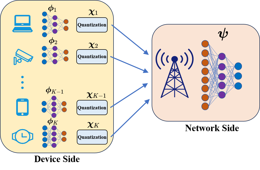
Figure 1: System model of collaborative intelligence between multiple devices and the network.

The input data of $K$ different mobile devices $(\boldsymbol{x}_{1},\dots,\boldsymbol{x}_{K})$ and the target variable $\boldsymbol{y}$ (e.g., label) are deemed as different realizations of the random variables $(X_{1},\dots,X_{K},Y)$ with joint distribution $p(\boldsymbol{x}_{1},\dots,\boldsymbol{x}_{K},\boldsymbol{y})$. Given the dataset $\{\boldsymbol{x}^{(m)}_{1},\dots,\boldsymbol{x}^{(m)}_{K}\}_{m=1}^{M}$, the goal of the system is to infer the targets $\{\boldsymbol{y}^{(m)}\}_{m=1}^{M}$. Upon receiving the input data $\boldsymbol{x}_{k}$, the $k$-th device extracts features from $\boldsymbol{x}_{k}$ and encodes them as $\boldsymbol{z}_{k}$. We collectively denote the feature extraction and encoding modules as the probability encoder $p_{\boldsymbol{\phi}_{k}}(\boldsymbol{z}_{k}|\boldsymbol{x}_{k})$, with the trainable DNN parameters $\boldsymbol{\phi}_{k}$ for the $k$-th device. To provide a clear probabilistic model for the devices, we employ the reparameterization trick [25]. We then model the conditional distribution $p_{\boldsymbol{\phi}_{k}}(\boldsymbol{z}_{k}|\boldsymbol{x}_{k})$ as a multivariate Gaussian distribution, that is,

$$p_{\boldsymbol{\phi}_{k}}(\boldsymbol{z}_{k}|\boldsymbol{x}_{k})=\mathcal{N}(\boldsymbol{z}_{k}|\boldsymbol{\mu}_{k},\boldsymbol{\Theta}_{k}).$$ (1)

Here, the covariance matrix $\boldsymbol{\Theta}_{k}$ is a diagonal matrix $\mathrm{diag}\{\theta_{k,1}^{2},\dots,\theta_{k,d}^{2}\}$. The mean vector $\boldsymbol{\mu}_{k}=(\mu_{k,1},\dots,\mu_{k,d})$ and the diagonal vector $\boldsymbol{\theta}_{k}=(\theta_{k,1},\dots,\theta_{k,d})$ are derived from the DNN-based function $\boldsymbol{\mu}_{k}(\boldsymbol{x}_{k},\boldsymbol{\phi}_{k})$ and $\boldsymbol{\theta}_{k}(\boldsymbol{x}_{k},\boldsymbol{\phi}_{k})$, respectively.

Next, the encoded feature $\boldsymbol{z}_{k}$ is quantized to $\tilde{\boldsymbol{z}}_{k}$ using our quantization function, which will be specified later, with all trainable parameters denoted as $\boldsymbol{\chi}_{k}$. The quantized feature $\tilde{\boldsymbol{z}}_{k}$ is then transmitted to the BS by the $k$-th device through the wireless channel. Without loss of generality, we consider the additive white Gaussian noise channel. Thus, $\hat{\boldsymbol{z}}_{k}=\tilde{\boldsymbol{z}}_{k}+\boldsymbol{\epsilon}_{k}$, where the noise $\boldsymbol{\epsilon}_{k}\sim\mathcal{N}(\boldsymbol{0},\sigma_{k}^{2}\boldsymbol{I})$ with its variance $\sigma_{k}^{2}$. The encoded feature $\boldsymbol{z}_{k}$, the quantized feature $\tilde{\boldsymbol{z}}_{k}$, and the received feature $\hat{\boldsymbol{z}}_{k}$ are instantiations of the random variables $Z_{k}$, $\tilde{Z}_{k}$, and $\hat{Z}_{k}$, respectively, allowing us to construct a Markov chain as

$$Y\leftrightarrow X_{k}\leftrightarrow Z_{k}\leftrightarrow\tilde{Z}_{k}\leftrightarrow\hat{Z}_{k}.$$ (2)

Here, the probability equation is given by $p(\hat{\boldsymbol{z}}_{k},\tilde{\boldsymbol{z}}_{k},\boldsymbol{z}_{k}|\boldsymbol{x}_{k})=p(\hat{\boldsymbol{z}}_{k}|\tilde{\boldsymbol{z}}_{k})p(\tilde{\boldsymbol{z}}_{k}|\boldsymbol{z}_{k})p_{\boldsymbol{\phi}_{k}}(\boldsymbol{z}_{k}|\boldsymbol{x}_{k})$. The network side performs inference tasks based on the received features $(\hat{\boldsymbol{z}}_{1},\dots,\hat{\boldsymbol{z}}_{K})$ from $K$ different devices, resulting in the inference output $\hat{\boldsymbol{y}}$. This output follows the conditional distribution $p_{\boldsymbol{\psi}}(\hat{\boldsymbol{y}}|\hat{\boldsymbol{z}}_{1:K})$, where $\boldsymbol{\psi}$ represents the parameters of the DNN employed at the network side.

II-B The ML-IB Scheme

For the system shown in Fig. 1, our objective is to design proper AI models for both the device side and the network side, which can ensure the accuracy of device-network collaborative AI tasks is high while the amount of data transmitted over wireless links is low. In the single device-network collaboration scenario, conventional IB theory offers an effective approach to achieve this objective [26]. Based on IB, we develop a multi-link information bottleneck (ML-IB) scheme for the scenario of intelligent collaboration between multiple devices and the network side. Initially, a novel performance metric is proposed, defined as:

$$\mathcal{C}_{\text{ML-IB}}=-I(Y;\hat{Z}_{1:K})+\sum_{k=1}^{K}\beta_{k}I(X_{k};\hat{Z}_{k}).$$ (3)

In this metric, the mutual information $I(Y;\hat{Z}_{1:K})$ reflects the information that received features of the network side $\hat{Z}_{1:K}=\{\hat{Z}_{1},\dots,\hat{Z}_{K}\}$ holds about the inference target variable $Y$, which can represent the inference accuracy. $I(X_{k};\hat{Z}_{k})$ assesses the retained information in $\hat{Z}_{k}$ given $X_{k}$ using the minimum description length [27], representing communication overhead. In addition, it can reflect the impact of encoding, quantization, and transmission processes on the input raw data. The tradeoff factor $\beta_{k}>0$ can be dynamically adjusted based on the specific conditions of the $k$-th channel. The summation $\sum_{1}^{K}\beta_{k}I(X_{k};\hat{Z}_{k})$ can represent the communication overhead of all of the $K$ wireless links. As such, a smaller $\mathcal{C}_{\text{ML-IB}}$ corresponds to a higher accuracy of the AI task and a lower communication overhead. The objective function can thus be formulated as

$$\min_{\{\boldsymbol{\phi}_{k}\}_{k=1}^{K},\{\boldsymbol{\chi}_{k}\}_{k=1}^{K},\boldsymbol{\psi}}\mathcal{C}_{\text{ML-IB}},$$ (4)

where we aim to determine the optimal AI models for the multiple devices (i.e., $\{\boldsymbol{\phi}_{k}\}_{k=1}^{K}$), the network side (i.e., $\boldsymbol{\psi}$), and the optimal quantization framework (i.e., $\{\boldsymbol{\chi}_{k}\}_{k=1}^{K}$) to achieve minimum $\mathcal{C}_{\text{ML-IB}}$.

II-C Variational Upper Bound of $\mathcal{C}_{\text{ML-IB}}$

To solve the problem (4), in this subsection, we focus on analyzing the expression of $\mathcal{C}_{\text{ML-IB}}$. In order to calculate the mutual information terms in $\mathcal{C}_{\text{ML-IB}}$, we need the conditional distribution $p(\boldsymbol{y}|\hat{\boldsymbol{z}}_{1:K})$ for $I(Y;\hat{Z}_{1:K})$ and the marginal distribution $p(\hat{\boldsymbol{z}}_{k})$ for $I(X_{k};\hat{Z}_{k})$. However, the high dimensionality of the input data poses inherent computational challenges, making accurate computation of these distributions difficult. To overcome this, we resort to variational approximation [23], [24], which is a popular technique used to approximate intractable distributions based on some adjustable parameters (e.g., weights in DNNs). We introduce variational distributions $\{r_{k}(\hat{\boldsymbol{z}}_{k})\}_{k=1}^{K}$ as approximations for $\{p(\hat{\boldsymbol{z}}_{k})\}_{k=1}^{K}$, where each $r_{k}(\hat{\boldsymbol{z}}_{k})$ is modeled as a centered isotropic Gaussian distribution [24], represented by $\mathcal{N}(\hat{\boldsymbol{z}}_{k}|\boldsymbol{0},\boldsymbol{I})$. Since the inference variable $\hat{Y}$ and the target variable $Y$ share the same range of values, we use $p_{\boldsymbol{\psi}}(\boldsymbol{y}|\hat{\boldsymbol{z}}_{1:K})$ as the variational approximation for $p(\boldsymbol{y}|\hat{\boldsymbol{z}}_{1:K})$, with $\boldsymbol{\psi}$ denoting the DNN parameters on the network side.

According to the non-negativity of the KL divergence $D_{\text{KL}}(p(\boldsymbol{y}|\hat{\boldsymbol{z}}_{1:K}),p_{\boldsymbol{\psi}}(\boldsymbol{y}|\hat{\boldsymbol{z}}_{1:K}))\geq 0$, we derive a lower bound for $I(Y;\hat{Z}_{1:K})$ as :

$$I(Y;\hat{Z}_{1:K})\geq\int p(\hat{\boldsymbol{z}}_{1:K},\boldsymbol{y})\log\frac{p_{\boldsymbol{\psi}}(\boldsymbol{y}|\hat{\boldsymbol{z}}_{1:K})}{p(\boldsymbol{y})}\,d\hat{\boldsymbol{z}}_{1:K}\,d\boldsymbol{y}.$$ (5)

Similarly, the non-negativity of $D_{\text{KL}}(p(\hat{\boldsymbol{z}}_{k}),r_{k}(\hat{\boldsymbol{z}}_{k}))$ allows us to deduce:

$$I(\hat{Z}_{k};X_{k})\leq\int p(\hat{\boldsymbol{z}}_{k},\boldsymbol{x}_{k})\log\frac{p_{\boldsymbol{\phi}_{k}}(\hat{\boldsymbol{z}}_{k}|\boldsymbol{x}_{k})}{r_{k}(\hat{\boldsymbol{z}}_{k})}d\hat{\boldsymbol{z}}_{k}d\boldsymbol{x}_{k}.$$ (6)

By combining (5) and (6), we can derive an upper bound of $\mathcal{C}_{\text{ML-IB}}$ ignoring a constant term $H(Y)$ as

$$\hat{\mathcal{C}}_{\text{ML-IB}} =\mathbb{E}_{p(\boldsymbol{x}_{1:K},\boldsymbol{y})}\Big{\{}\mathbb{E}_{p(\hat{\boldsymbol{z}}_{1:K}|\boldsymbol{x}_{1:K})}[-\log p_{\boldsymbol{\psi}}(\boldsymbol{y}|\hat{\boldsymbol{z}}_{1:K})]$$ (7)

$$\quad+\!\sum_{k=1}^{K}\beta_{k}D_{\text{KL}}(p_{\boldsymbol{\phi}_{k}}(\hat{\boldsymbol{z}}_{k}|\boldsymbol{x}_{k})||r_{k}(\hat{\boldsymbol{z}}_{k}))\Big{\}}.$$

III Computable ML-IB Model

The numerical calculation of the upper bound $\hat{\mathcal{C}}_{\text{ML-IB}}$ is still difficult, due to the intractable KL divergence term when the quantization units are considered.

Following the idea in [28], we design the quantization unit. Our quantizer allows more flexible control of the quantization bit depth, breakpoint, and amplitude, which takes real-world deployment into account. To tackle the upper bound $\hat{\mathcal{C}}_{\text{ML-IB}}$, we derive a manageable approximation of $\hat{\mathcal{C}}_{\text{ML-IB}}$ by applying the Log-Sum Inequality, enabling the computability of our ML-IB scheme. Furthermore, we provide an error bound for the approximation to provide a theoretical guarantee.

III-A Quantization Design

We denote the encoded vector $\boldsymbol{z}_{k}=(z_{k,1},\dots,z_{k,d})\in\mathbb{R}^{d}$. For the quantizer, we utilize a piecewise step function defined by:

$$\tilde{z}_{k,i}=\sum_{t=1}^{T}\frac{a_{k,t}^{2}}{\sum_{t=1}^{T}a_{k,t}^{2}}\text{sgn}(z_{k,i}-b_{k,t}),\quad i=1,\dots,d,$$ (8)

where $T$ reflects the number of quantization bits, $a_{k,t}$ represents the amplitude and $b_{k,t}$ is the breakpoint. Then the quantizer transforms each dimension $z_{k,i}$ of the vector $\boldsymbol{z}_{k}$ into $\tilde{z}_{k,i}$, which can take only $T+1$ discrete values between $-1$ and $1$. For brevity, let us denote $c_{k,1}=-1,c_{k,2}=\frac{a_{k,1}^{2}-\sum_{t=2}^{T}a_{k,t}^{2}}{\sum_{t=1}^{T}a_{k,t}^{2}},\dots,c_{k,T+1}=1$. We specify the quantization function for $\tilde{z}_{k,i}$ as follows:

$$\tilde{z}_{k,t}=\begin{cases}c_{k,1},&\text{if}~{}z_{k,i}<b_{k,1},\\ c_{k,2},&\text{if}~{}b_{k,1}\leq z_{k,i}<b_{k,2},\\ &\cdots\\ c_{k,T+1}&\text{if}~{}z_{k,i}\geq b_{k,T}.\\ \end{cases}$$ (9)

As introduced in Section II-A, each component ${Z}_{k,i}$ of the variable ${Z}_{k}$ is conditionally independent given $X_{k}$. Consequently, the conditional cumulative distribution function of $Z_{k,i}$, conditioned on $X_{k}$ is obtained as

$$F_{Z_{k,i}|X_{k}}(c) =P(Z_{k,i}<c|X_{k})$$ (10)

$$=\frac{1}{2}\left[1+\text{erf}\left(\frac{c-\mu_{k,i}}{\theta_{k,i}\sqrt{2}}\right)\right].$$

From above, we denote $P(\tilde{Z}_{k,i}=c|X_{k})=P_{k,i}(c)$ and derive the conditional probability mass function of the quantized variable $\tilde{Z}_{k,i}$ given $X_{k}$, as described below:

$$\!\!P_{k,i}(c)\!=\!\begin{cases}F_{Z_{k,i}|X_{k}}(b_{k,1}),&\text{if}~{}c=c_{k,1},\\ F_{Z_{k,i}|X_{k}}(b_{k,2})-F_{z_{k,i}|\boldsymbol{x}_{k}}(b_{k,1}),&\text{if}~{}c=c_{k,2},\\ &\cdots\\ 1-F_{Z_{k,i}|X_{k}}(b_{k,T}),&\text{if}~{}c=c_{k,T+1}.\\ \end{cases}$$ (11)

Then, we consider a soft quantization function, which is defined by the following equation for each component $\tilde{z}_{k,i}$:

$$\tilde{z}_{k,i}=\sum_{t=1}^{T}\frac{a^{2}_{k,t}}{\sum_{t=1}^{T}a_{k,t}^{2}}\arctan(\gamma(z_{k,i}-b_{k,t})).$$ (12)

In this formulation, the parameters $a_{k,t}$ and $b_{k,t}$ for $t=1$ to $T$, belonging to $\boldsymbol{\chi}_{k}$, are adaptable during training to reflect real-time conditions. This makes the quantization function effectively adapt to various channels and different transmission devices.

Given $\hat{\boldsymbol{z}}_{k}=\tilde{\boldsymbol{z}}_{k}+\boldsymbol{\epsilon}_{k}$ with $\boldsymbol{\epsilon}_{k}\sim\mathcal{N}(0,\sigma_{k}^{2}I)$, each component $\hat{z}_{k,i}$ independently follows a conditionally independent Gaussian mixture conditional on $X_{k}$, for $i=1,\dots,d$. To be specific, the conditional probability density function for $\hat{z}_{k,i}$ is expressed as:

$$p_{\boldsymbol{\phi}_{k}}(\hat{z}_{k,i}|\boldsymbol{x}_{k})=\sum_{t=1}^{T+1}P_{k,i}(c_{k,t})f_{\epsilon}(\hat{z}_{k,i}-c_{k,t}),$$ (13)

where $f_{\epsilon}$ denotes the density function of $\epsilon_{k,i}$, and $\epsilon_{k,i}=\hat{z}_{k,i}-c_{k,t}$ follows a normal distribution $\mathcal{N}(0,\sigma_{k}^{2})$.

III-B Approximation of Variational Upper bound

The computation of the variational bound $\hat{\mathcal{C}}_{\text{ML-IB}}$, involving the integral of logarithms of a Gaussian mixture as indicated by $p_{\boldsymbol{\phi}_{k}}(\hat{z}_{k,i}|\boldsymbol{x}_{k})$ in (13), presents a notable challenge. In this subsection, We produce an approximation of $\hat{\mathcal{C}}_{\text{ML-IB}}$ with a theoretical guarantee, making our ML-IB scheme computable.

To begin, we define

$$D^{*}_{\text{KL}}(p_{\boldsymbol{\phi}_{k}}(\hat{\boldsymbol{z}}_{k}|\boldsymbol{x}_{k})||r_{k}(\hat{\boldsymbol{z}}_{k}))$$ (14)

$$\triangleq-H(\tilde{Z}_{k})+\sum_{i=1}^{d}\Big{\{}\log(T+1)-\frac{1}{2}\log{\sigma_{k}^{2}}$$

$$\qquad\qquad\qquad\qquad+\frac{1}{2}\sigma_{k}^{2}-\frac{1}{2}+\sum_{t=1}^{T+1}P_{k,i}(c_{k,t})(c_{k,t})^{2}\Big{\}},$$

and

$$\mathcal{C}_{\text{QML-IB}} \triangleq\!\mathbb{E}_{p(\boldsymbol{x}_{1:K},\boldsymbol{y})}\Big{\{}\mathbb{E}_{p(\hat{\boldsymbol{z}}_{1:K}|\boldsymbol{x}_{1:K})}[-\log p_{\boldsymbol{\psi}}(\boldsymbol{y}|\hat{\boldsymbol{z}}_{1:K})]$$ (15)

$$\quad\!+\!\sum_{k=1}^{K}\beta_{k}D^{*}_{\text{KL}}(p_{\boldsymbol{\phi}_{k}}(\hat{\boldsymbol{z}}_{k}|\boldsymbol{x}_{k})||r_{k}(\hat{\boldsymbol{z}}_{k}))\Big{\}}.$$

Lemma 1.

The $D_{\text{KL}}^{*}$ defined in (14) serves as an upper bound for the KL divergence within $\hat{\mathcal{C}}_{\text{ML-IB}}$:

$$D_{\text{KL}}(p_{\boldsymbol{\phi}_{k}}(\hat{\boldsymbol{z}}_{k}|\boldsymbol{x}_{k})||r_{k}(\hat{\boldsymbol{z}}_{k}))\leq D^{*}_{\text{KL}}(p_{\boldsymbol{\phi}_{k}}(\hat{\boldsymbol{z}}_{k}|\boldsymbol{x}_{k})||r_{k}(\hat{\boldsymbol{z}}_{k}))$$ (16)

Proof:

The challenge in evaluating the KL divergence term within arises from the integral involving the logarithms of the sum of Gaussians. We address this issue by employing the Log-Sum Inequality [27], as elaborated in Appendix A. ∎

Theorem 1.

For the variational upper bound $\hat{\mathcal{C}}_{\text{ML-IB}}$ in (7) and $\mathcal{C}_{\text{QML-IB}}$ in (15), we establish that:

$$\hat{\mathcal{C}}_{\text{ML-IB}}\leq\mathcal{C}_{\text{QML-IB}}.$$ (17)

Proof:

Referencing Lemma 1, it is established that $D^{*}_{\text{KL}}$ surpasses the KL divergence component in $\hat{\mathcal{C}}_{\text{ML-IB}}$, thereby validating the inequality in (17). ∎

Following Theorem 1, we derive an approximation for the variational upper bound $\hat{\mathcal{C}}_{\text{ML-IB}}$, denoted as $\mathcal{C}_{\text{QML-IB}}$, which can be easily and quickly obtained during training. According to Monte Carlo sampling, we can obtain an unbiased estimate of the gradient for the optimization function in (15) and proceed with its optimization. Specifically, during the training process, given a mini-batch of data $\{(\boldsymbol{x}_{1}^{(m)},\boldsymbol{x}_{2}^{(m)},\dots,\boldsymbol{x}_{K}^{(m)})\}_{m=1}^{M}$ and sampling the channel noise $L$ times for each transmission, we acquire the following empirical estimates:

$$\mathcal{C}_{\text{QML-IB}} \simeq\frac{1}{M}\sum_{m=1}^{M}\frac{1}{L}\sum_{l=1}^{L}\left\{-\log p_{\boldsymbol{\psi}}(\boldsymbol{y}^{(m)}|\hat{\boldsymbol{z}}^{(m)}_{1:K,l})\vphantom{\sum_{k=1}^{K}}\right.$$ (18)

$$\quad\left.+\sum_{k=1}^{K}\beta_{k}D_{\text{KL}}\left(p_{\boldsymbol{\phi}_{k}}(\hat{\boldsymbol{z}}_{k}|\boldsymbol{x}_{k})\middle\|r_{k}(\hat{\boldsymbol{z}}_{k})\right)\right\},$$

where $\hat{\boldsymbol{z}}_{k,l}^{(m)}=\boldsymbol{z}_{k}^{(m)}+\epsilon_{k,l}^{(m)}$, and $\epsilon_{k,l}^{(m)}\sim\mathcal{N}(\boldsymbol{0},\sigma_{k}^{2}I)$.

Building on this, we devise the quantized multi-link information bottleneck (QML-IB) algorithm to generate AI models for collaborative intelligence in a multi-device scenario, which is summarized in Algorithm 1.

Theorem 2.

The discrepancy between the approximation and the KL divergence is given by:

$$D^{*}_{\text{KL}}(p_{\boldsymbol{\phi}_{k}}(\hat{\boldsymbol{z}}_{k}|\boldsymbol{x}_{k})||r_{k}(\hat{\boldsymbol{z}}_{k}))-D_{\text{KL}}(p_{\boldsymbol{\phi}_{k}}(\hat{\boldsymbol{z}}_{k}|\boldsymbol{x}_{k})||r_{k}(\hat{\boldsymbol{z}}_{k}))$$ (19)

$$\leq\frac{2Td}{T+1}C+2d\delta$$

In this context, $T$ denotes the number of breakpoints in the quantization function and $d$ represents the dimension of the vector $\hat{\boldsymbol{z}}_{k}$. The constants $C$ and $\delta$ are computable and depend exclusively on the probability mass function of $\tilde{Z}_{k}$ given $X_{k}$, as well as the channel noise $\sigma_{k}^{2}$.

Proof:

By customizing the error analysis to two distinct ranges of $\hat{z}_{k,i}$, we bound the aforementioned discrepancy as outlined in Appendix B. ∎

Theorem 2 elucidates the validity of using $D_{\text{KL}}^{*}$ as an approximation for $D_{\text{KL}}$. It demonstrates that the discrepancy between them is under control by the values of $T$ and $d$.

Algorithm 1 Quantized multi-link information bottleneck

1:Training dataset $\mathcal{D}$, number of iterations $P$, number of devices $K$, number of channel noise samples $L$, number of breakpoints $T$, batch size $M$, channel noise variance $\{\sigma_{k}^{2}\}_{k=1}^{K}$.

2:The optimized parameters $\{\boldsymbol{\phi}_{k}\}_{k=1}^{K}$, $\{\boldsymbol{\chi}_{k}\}_{k=1}^{K}$ and $\boldsymbol{\psi}$.

3:for epoch $p=1$ to $P$ do

4:     Select a mini-batch of data $\{(\boldsymbol{x}_{1}^{(m)},\dots,\boldsymbol{x}_{K}^{(m)})\}_{m=1}^{M}$

5:     for $k=1$ to $K$ and $m=1$ to $M$ do

6:         Compute the feature vector $\boldsymbol{z}_{k}^{(m)}$ based on (1)

7:         Compute the quantized vector $\tilde{\boldsymbol{z}}_{k}^{(m)}$ based on (12)

8:         Sample the noise $\{\epsilon_{k,l}^{(m)}\}_{l=1}^{L}\sim\mathcal{N}(\boldsymbol{0},\sigma_{k}^{2}I)$

9:         Compute the received vector based on

10:   $\hat{\boldsymbol{z}}_{k,l}^{(m)}=\tilde{\boldsymbol{z}}_{k}^{(m)}+\epsilon_{k,l}^{(m)}$      

11:     Compute the KL-divergence based on (14)

12:     Compute the loss $\mathcal{C}_{\text{QML-IB}}$ based on (18)

13:     Update parameters through backpropagation

IV Numerical Results and Discussions

This section evaluates the performance of our proposed algorithm in device-network collaborative intelligence.

IV-A Experimental Settings

We selected the MNIST[29] and CIFAR-10[30] as benchmark datasets for classification tasks. We conducted numerical experiments for both of our proposed QML-IB algorithm and a benchmark. With limited research in multi-link collaborative intelligence, we select the method VDDIB-SR[18] as our baseline for comparison. Our algorithm and the baseline both feature a quantization framework. Note that to ensure a comprehensive experimental comparison, we simulate their non-quantized versions as well.

Following the method in [31], we split each image into $K$ equal, non-overlapping sub-images, with each device assigned a sub-image. The hyperparameters $\beta_{k}$ (for $k=1,\dots,K$) in (3) are set within the range of $[10^{-5},10^{-1}]$, and the grid search is utilized to determine their optimal values for the MNIST and CIFAR-10 datasets [32]. Following [28], we set the constant $\gamma$ in (12) to 10. For the constant $T$, set at 15, further discussion is available in Appendix C. For consistency, we followed the setup from [26] with a 12.5kHz bandwidth and 9,600 baud symbol rate. We adopt the same neural network backbone for all algorithms, as depicted in Tables I and II. The Peak Signal-to-Noise Ratio (PSNR) for channel $k$ is:

$$\text{PSNR}=10\log\left(\frac{P_{\text{max}}}{\sigma_{k}^{2}}\right)\text{dB},$$ (20)

where $P_{\text{max}},$ the signal’s maximum power, is set to 1 in our experiments, as each component of the encoded vector $z_{k}$ is limited to $|z_{k,i}|\leq 1$.

TABLE I: THE DNN ARCHITECTURE FOR MNIST CLASSIFICATION

	Layer	Outputs
Device-side Network	FC Layer + Tanh	d
Server-side Network	FC Layer + ReLU	1024
	FC Layer + ReLU	256
	FC Layer + Softmax	10

TABLE II: THE DNN ARCHITECTURE FOR CIFAR-10 CLASSIFICATION.

Network	Layer	Outputs
Device-side Network	Conv Layer $\times$ 2 + ResNet Block	$128\times 32\times 32$
	Conv Layer $\times$ 2 + ResNet Block	$512\times 4\times 4$
	Conv Layer	$4\times 4\times 4$
	Reshape + FC Layer + Tanh	$d$
Server-side Network	FC Layer + Reshape	$4\times 4\times 4$
	Conv Layer$\times$ 2	$512\times 4\times 4$
	ResNet Block $\times$ 2	$512\times 4\times 4$
	Pooling Layer	$512$
	FC Layer + Softmax	$10$

IV-B Experimental Results

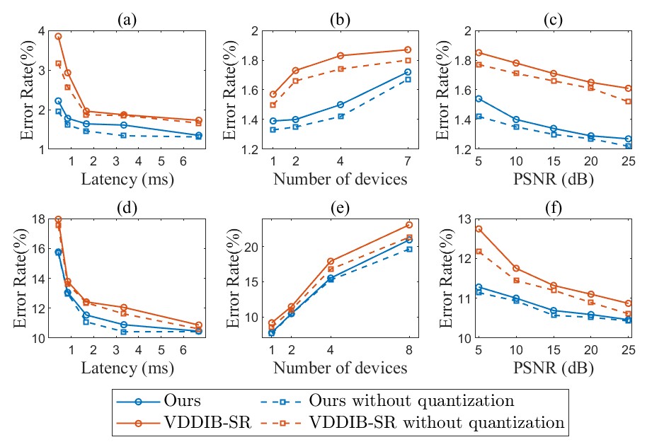
Figure 2: Performance comparison between our algorithm and VDDIB-SR in different experimental settings. Evaluations on MNIST Dataset in Figs. 2(a), (b), (c) and on CIFAR-10 Dataset in Figs. 2(d), (e), (f).

In our experiments, we evaluate the error rate of our algorithm and the benchmark VDDIB-SR for processing AI tasks, in terms of three key aspects: communication latency, number of devices, and PSNR. First, we standardize the PSNR at 10 dB in a two-device configuration to evaluate the algorithm performance under varying communication latencies, detailed in Figs. 2(a) and (d). We then evaluate how well the algorithms adapt to different numbers of devices while keeping the communication latency below 6 ms, as shown in Figs. 2(b) and (e). Finally, to test the robustness of the algorithms, we vary the PSNR while maintaining the device count at 2, observing their performance across different channel noise in Figs. 2(c) and (f).

Results from Fig. 2 show that our algorithm consistently exhibits a lower error rate than VDDIB-SR in various experimental scenarios, indicating superior performance in multi-device collaborative settings. This confirms the superiority of the ML-IB method and the well-designed performance metric $\mathcal{C}_{\text{ML-IB}}$. Specifically, Figs. 2(a) and (d) show that our algorithm achieves lower error rates with reduced latency. Figs. 2(b) and (e) demonstrate its ability to effectively coordinate an increasing number of devices. In addition, Figs. 2(c) and (f) highlight its consistent outperformance under varying PSNR, validating its robustness to different channel conditions.

Furthermore, experimental results indicate that our algorithm maintains an error rate close to its unquantized version. This reflects that our quantization, tailored to real-world scenarios and compatible with digital communication systems, incurs only negligible performance loss. Notably, our algorithm, even with the quantization scheme applied, still outperforms the baseline’s non-quantized version. This underscores the ability of our QML-IB algorithm to provide strong performance assurance and confirms its significant practical value.

V Conclusion

In this work, we investigate the establishment of collaborative intelligence across multiple wireless links. We introduce an ML-IB scheme with a novel performance metric $\mathcal{C}_{\text{ML-IB}}$. To fulfill practical communication requirements, we design a quantizer that offers adaptable management of quantization parameters, including bit depth, breakpoint, and amplitude. Using variational methods and the Log-Sum Inequality, we derive an approximation for $\mathcal{C}_{\text{ML-IB}}$ to make the ML-IB scheme computable. We also provide an error analysis to demonstrate the validity of this approximation. On this basis, we propose the QML-IB algorithm for AI model generation. Numerical experiments validate the effectiveness of our algorithm and the superiority of the performance metric. We want to stress that our proposed approach may be applicable to various communication channels, not just the additive white Gaussian noise channel that we discussed in this paper. For instance, it could be used on the Rayleigh Fading Channel and the Rician Fading Channel [33]. This is an interesting topic that warrants further research.

Appendix A Proof of Lemma 1

Considering the conditional independence of $\hat{z}_{k,i}$ and the isotropy of the variational marginal distribution, we have:

$$D_{\text{KL}}(p_{\boldsymbol{\phi}_{k}}(\hat{\boldsymbol{z}}_{k}|\boldsymbol{x}_{k})||r_{k}(\hat{\boldsymbol{z}}_{k}))=\int p_{\boldsymbol{\phi}_{k}}(\hat{\boldsymbol{z}}_{k}|\boldsymbol{x}_{k})\log\frac{p_{\boldsymbol{\phi}_{k}}(\hat{\boldsymbol{z}}_{k}|\boldsymbol{x}_{k})}{r(\hat{\boldsymbol{z}}_{k})}d\hat{\boldsymbol{z}}_{k}$$

$$=\sum_{i=1}^{d}\int p_{\boldsymbol{\phi}_{k}}(\hat{z}_{k,i}|\boldsymbol{x}_{k})\log\frac{p_{\boldsymbol{\phi}_{k}}(\hat{z}_{k,i}|\boldsymbol{x}_{k})}{r_{k}(\hat{z}_{k,i})}d\hat{z}_{k,i}$$ .

Here, $p_{\boldsymbol{\phi}_{k}}(\hat{z}_{k,i}|\boldsymbol{x}_{k})=\sum_{t=1}^{T+1}P_{k,i}(c_{k,t})f_{\epsilon}(\hat{z}_{k,i}-c_{k,t})$ and $r_{k}(\hat{\boldsymbol{z}}_{k})=\mathcal{N}(\hat{\boldsymbol{z}}_{k}|\boldsymbol{0},\boldsymbol{I})$. Then we define $a_{i,t}=P_{k,i}(c_{k,t})f_{\epsilon}(\hat{z}_{k,i}-c_{k,t})$ and $b_{i,t}=\frac{1}{T+1}r_{k}(\hat{\boldsymbol{z}}_{k})$. Applying the Log-Sum Inequality [27], we have:

$$\left(\sum_{t=1}^{T+1}a_{i,t}\right)\log\frac{\sum_{t=1}^{T+1}a_{i,t}}{\sum_{t=1}^{T+1}b_{i,t}}\leq\sum_{t=1}^{T+1}a_{t}\log\frac{a_{i,t}}{b_{i,t}}.$$ (21)

Consequently, this leads to the inequality:

$$\sum_{t=1}^{T+1}P_{k,i}(c_{k,t})f_{\epsilon}(\hat{z}_{k,i}-c_{k,t})\log\frac{\sum_{t=1}^{T+1}P_{k,i}(c_{k,t})f_{\epsilon}(\hat{z}_{k,i}-c_{k,t})}{r(\hat{z}_{k,i})}$$

$$\leq\sum_{t=1}^{T+1}P_{k,i}(c_{k,t})f_{\epsilon}(\hat{z}_{k,i}-c_{k,t})\log\frac{P_{k,i}(c_{k,t})f_{\epsilon}(\hat{z}_{k,i}-c_{k,t})}{\frac{1}{T+1}r(\hat{z}_{k,i})}.$$

Applying the formula for calculating the cross-entropy between two Gaussian distributions and integrating the right-hand side of the inequality, we derive

$$\int p_{\boldsymbol{\phi}_{k}}(\hat{z}_{k,i}|\boldsymbol{x}_{k})\log\frac{p_{\boldsymbol{\phi}_{k}}(\hat{z}_{k,i}|\boldsymbol{x}_{k})}{r_{k}(\hat{z}_{k,i})}d\hat{z}_{k,i}$$ (22)

$$\leq-H(\tilde{Z}_{k,i})-\frac{1}{2}\log{\sigma_{k}^{2}}+\frac{1}{2}\sigma_{k}^{2}-\frac{1}{2}+\sum_{t=1}^{T+1}p_{k,i}(c_{t})(c_{t})^{2},$$

Next, we sum over both sides of inequality (22) for $i=1$ to $d$, leading to inequality (16) and completing the proof.

Appendix B Proof of Theorem 2

Let $C_{i,t}=(T+1)P_{k,i}(c_{k,t})\frac{1}{\sigma_{k}}e^{\frac{-c_{k,t}^{2}}{2(1-\sigma_{k}^{2})}}$ for $i=1,\ldots,d$ and $t=1,\ldots,T+1$, with $C_{\text{max}}=\max_{i,t}\{C_{i,t}\}$ and $C_{\text{min}}=\min_{i,t}\{C_{i,t}\}$. Define $C_{0}=\max(||\log C_{\text{min}}||,||\log C_{\text{max}}||)$, $\varepsilon=\frac{(1+3\sigma_{k}+\frac{1}{1-\sigma_{k}^{2}})^{2}}{\frac{2\sigma_{k}^{2}}{1-\sigma_{k}^{2}}}$ and $\delta=\max(\frac{1}{e},C_{\text{max}}e^{-\varepsilon}\log(C_{\text{max}}e^{-\varepsilon}))$. We continue using the notation from Theorem 1, defining $f(x)=x\log x$, $\alpha_{i,t}=\frac{b_{i,t}}{\sum_{t=1}^{T+1}b_{i,t}}$, and $\beta_{i,t}=\frac{a_{i,t}}{b_{i,t}}$. Thus,

$$D^{*}_{\text{KL}}(p_{\boldsymbol{\phi}_{k}}(\hat{\boldsymbol{z}}_{k}|\boldsymbol{x}_{k})||r_{k}(\hat{\boldsymbol{z}}_{k}))-D_{\text{KL}}(p_{\boldsymbol{\phi}_{k}}(\hat{\boldsymbol{z}}_{k}|\boldsymbol{x}_{k})||r_{k}(\hat{\boldsymbol{z}}_{k}))$$

$$=\sum_{i=1}^{d}\int(\sum_{t=1}^{T+1}{b_{i,t}})(\sum_{t=1}^{T+1}{\alpha_{i,t}}f(\beta_{i,t})-f(\sum_{t=1}^{T+1}\alpha_{i,t}\beta_{i,t}))d\hat{z}_{k,i}.$$

Given the expression of $\beta_{i,t}$:

$$\beta_{i,t}=\frac{a_{i,t}}{b_{i,t}}=(T+1)P_{k,i}(c_{k,t})\frac{1}{\sigma_{k}}e^{\frac{-c_{k,t}^{2}}{2(1-\sigma_{k}^{2})}}e^{-\frac{(\hat{z}_{k,i}-\frac{c_{k,t}}{1-\sigma_{k}^{2}})^{2}}{\frac{2\sigma_{k}^{2}}{1-\sigma_{k}^{2}}}},$$

when $\hat{z}_{k,i}\in(-1-3\sigma_{k},1+3\sigma_{k})$, the bounds for $\beta_{i,t}$ can be described as:

$$C_{i,t}e^{-\varepsilon}\leq\beta_{i,t}\leq C_{i,t}.$$ (23)

Furthermore,

$$||(\sum_{t=1}^{T+1}{b_{i,t}})(\sum_{t=1}^{T+1}{\alpha_{i,t}}f(\beta_{i,t})-f(\sum_{t=1}^{T+1}\alpha_{i,t}\beta_{i,t}))||$$

$$\leq||\sum_{t=1}^{T+1}{b_{i,t}}||\cdot\sum_{t=1}^{T+1}\left(||\alpha_{i,t}||\cdot||f(\beta_{i,t})-f(\sum_{t=1}^{T+1}\alpha_{i,t}\beta_{i,t})||\right).$$

Applying the Lagrange median theorem, we find

$$||f(\beta_{i,t})-f(\sum_{t=1}^{T+1}\alpha_{i,t}\beta_{i,t})||=||f^{{}^{\prime}}(\xi)||\cdot||\beta_{i,t}-\sum_{t=1}^{T+1}\alpha_{i,t}\beta_{i,t})||$$

$$\leq||f^{{}^{\prime}}(\xi)||\sum_{j=1}^{T+1}\left(||\alpha_{i,j}||\cdot||\beta_{i,t}-\beta_{i,j}||\right)$$

$$\leq\frac{1}{T+1}||f^{{}^{\prime}}(\xi)||(\sum_{j\neq t}||\beta_{i,j}||+T||\beta_{i,t}||),$$

where $\xi\in[\beta_{i,t},\sum_{t=1}^{T+1}\alpha_{i,t}\beta_{i,t})]$ or $\xi\in[\sum_{t=1}^{T+1}\alpha_{i,t}\beta_{i,t},\beta_{i,t})]$. Given $f(x)=x\log x$ with the derivative $f^{{}^{\prime}}(x)=\log x+1$ and considering the range of $\beta_{i,t}$ as defined in (23), we can deduce that

$$||f^{{}^{\prime}}(\xi)||<C_{0}+\log\varepsilon+1.$$

Consequently,

$$||(\sum_{t=1}^{T+1}{b_{i,t}})(\sum_{t=1}^{T+1}{\alpha_{i,t}}f(\beta_{i.t})-f(\sum_{t=1}^{T+1}\alpha_{i,t}\beta_{i,t}))||$$

$$\leq\frac{2T}{T+1}(C_{0}+\log\varepsilon+1)(\sum_{t=1}^{T}a_{i,t}).$$

Then

$$\int_{-1-3\sigma_{k}}^{1+3\sigma_{k}}(\sum_{t=1}^{T+1}{b_{i,t}})(\sum_{t=1}^{T+1}{\alpha_{i,t}}f(\beta_{i,t})-f(\sum_{t=1}^{T+1}\alpha_{i,t}\beta_{i,t}))d\hat{z}_{k,i}$$ (24)

$$\leq\frac{2T}{T+1}(C_{0}+\log\varepsilon+1).$$

For $\hat{z}_{k,i}$ within the ranges $(-\infty,-1-3\sigma_{k})$ or $(1+3\sigma_{k},\infty)$, it is deduced that $0<\beta_{i,t}\leq C_{i,t}e^{-\varepsilon}$. This implies $|f(\beta_{i,t})|$ is less than the maximum of ${\frac{1}{e},|C_{i,t}e^{-\varepsilon}\log C_{i,t}e^{-\varepsilon}|}$, which in turn is bounded above by $\delta$, applicable for $i=1,\dots,d$ and $t=1,\dots,T+1$. So

$$\left(\int_{-\infty}^{-1-3\sigma_{k}}+\int_{1+3\sigma_{k}}^{\infty}\right)$$ (25)

$$\quad(\sum_{t=1}^{T+1}{b_{i,t}})\left(\sum_{t=1}^{T+1}{\alpha_{i,t}}f(\beta_{i,t})-f\left(\sum_{t=1}^{T+1}\alpha_{i,t}\beta_{i,t}\right)\right)d\hat{z}_{k,i}$$

$$\leq 2\delta.$$

Therefore, based on the inequalities (24) and (25), we can deduce that:

$$\int(\sum_{t=1}^{T+1}{b_{i,t}})(\sum_{t=1}^{T+1}{\alpha_{i,t}}f(\beta_{i,t})-f(\sum_{t=1}^{T+1}\alpha_{i,t}\beta_{i,t}))d\hat{z}_{k,i}$$ (26)

$$\leq\frac{2T}{T+1}(C_{0}+\log\varepsilon+1)+2d\delta.$$

We denote $C=C_{0}+\log\varepsilon+1$, then the actual error can be expressed as:

$$D^{*}_{\text{KL}}(p_{\boldsymbol{\phi}_{k}}(\hat{\boldsymbol{z}}_{k}|\boldsymbol{x}_{k})||r_{k}(\hat{\boldsymbol{z}}_{k}))-D_{\text{KL}}(p_{\boldsymbol{\phi}_{k}}(\hat{\boldsymbol{z}}_{k}|\boldsymbol{x}_{k})||r_{k}(\hat{\boldsymbol{z}}_{k}))$$ (27)

$$\leq\frac{2Td}{T+1}C+2d\delta.$$

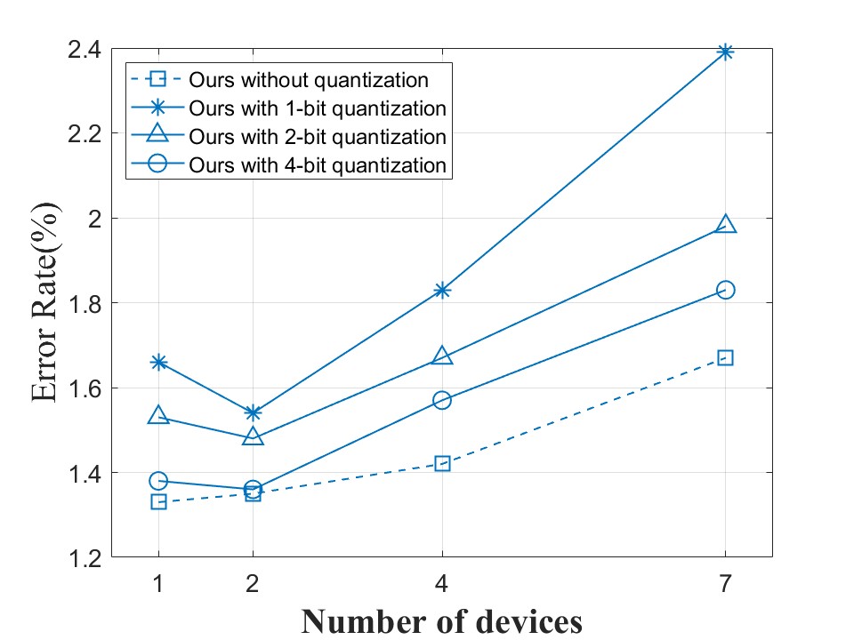
(a) MNIST dataset.

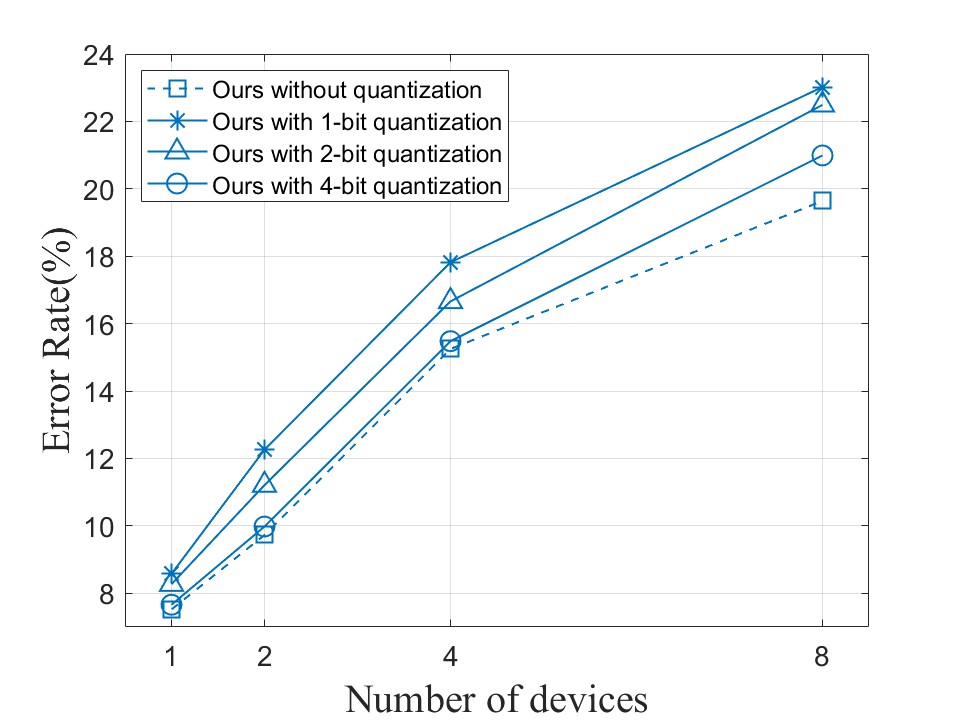
(b) CIFAR-10 dataset.

Figure 3: Impact of the quantization bit depth on performance

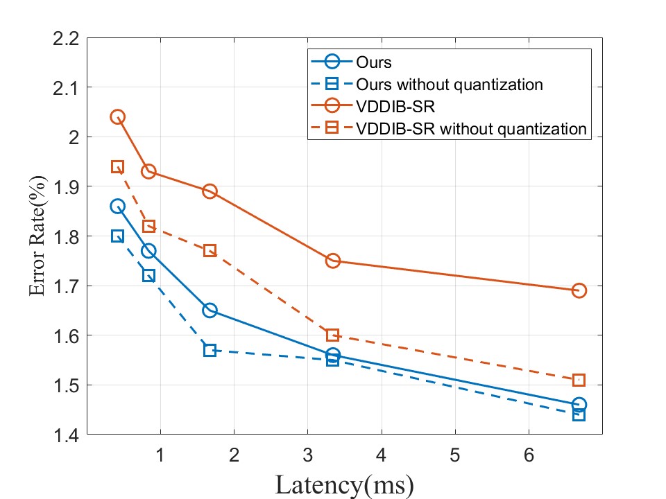
(a) MNIST dataset.

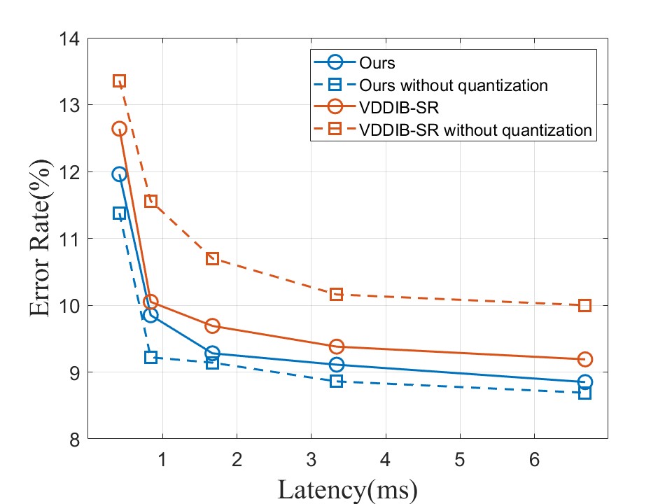
(b) CIFAR-10 dataset.

Figure 4: Performance in partial overlap of original input data

Appendix C Ablation Study

In this subsection, we investigate the impact of our quantization framework on inference performance with different numbers of quantization bits. Furthermore, we further analyze the performance of our algorithm when the raw data received by different devices partially overlap.

C-A Number of Quantization Bits

We set the PSNR to 10 dB and the communication latency remains below 6 ms. Within our proposed quantization framework, we compare four versions: quantization with 2, 4, and 16 discrete values, corresponding to 1, 2, and 4 quantization bits, respectively, and a version without quantization. As illustrated in Fig. 3, it is evident that the error rate decreases as the number of discrete quantization values increases, progressively converging towards the performance of the non-quantized version. Remarkably, with only a 4-bit quantization of our framework, the error is already very close to the version without quantization. This clearly demonstrates that the performance degradation introduced by our quantization is negligible.

C-B Scenario with Overlapping Raw Input Data

We divide each image into $K$ equal sub-images, ensuring a 50% overlap between adjacent sub-images, with each one allocated to a distinct device, as detailed in Fig. 4. When there is partial overlap in the input data, the error rate generated by our algorithm is consistently lower than the baseline, further demonstrating the applicability of our algorithm in diverse collaborative intelligence scenarios. Additionally, we find that in scenarios where data overlap occurs, the error rate of our algorithm is lower than in non-overlapping cases. This indicates that the intersection of original input data across different devices can better facilitate the extraction of task-relevant information, consequently enhancing the performance of AI tasks.

References

• [1] X. Hou, S. Dey, J. Zhang, and M. Budagavi, “Predictive view generation to enable mobile 360-degree and vr experiences,” in Proceedings of the 2018 Morning Workshop on Virtual Reality and Augmented Reality Network, 2018, pp. 20–26.
• [2] C. Anthes, R. J. García-Hernández, M. Wiedemann, and D. Kranzlmüller, “State of the art of virtual reality technology,” in 2016 IEEE aerospace conference.   IEEE, 2016, pp. 1–19.
• [3] S. K. Gaikwad, B. W. Gawali, and P. Yannawar, “A review on speech recognition technique,” International Journal of Computer Applications, vol. 10, no. 3, pp. 16–24, 2010.
• [4] K. Chowdhary and K. Chowdhary, “Natural language processing,” Fundamentals of artificial intelligence, pp. 603–649, 2020.
• [5] I. RECOMMENDATION, “Framework and overall objectives of the future development of imt for 2030 and beyond,” tech. rep., International Telecommunication Union (ITU) Recommendation (ITU-R), Tech. Rep., 2023.
• [6] K. B. Letaief, Y. Shi, J. Lu, and J. Lu, “Edge artificial intelligence for 6G: Vision, enabling technologies, and applications,” IEEE Journal on Selected Areas in Communications, vol. 40, no. 1, pp. 5–36, 2021.
• [7] E. C. Strinati and S. Barbarossa, “6G networks: Beyond shannon towards semantic and goal-oriented communications,” Computer Networks, vol. 190, p. 107930, 2021.
• [8] G. Zhu, D. Liu, Y. Du, C. You, J. Zhang, and K. Huang, “Toward an intelligent edge: Wireless communication meets machine learning,” IEEE communications magazine, vol. 58, no. 1, pp. 19–25, 2020.
• [9] M. Jankowski, D. Gündüz, and K. Mikolajczyk, “Wireless image retrieval at the edge,” IEEE Journal on Selected Areas in Communications, vol. 39, no. 1, pp. 89–100, 2020.
• [10] Y. Kang, J. Hauswald, C. Gao, A. Rovinski, T. Mudge, J. Mars, and L. Tang, “Neurosurgeon: Collaborative intelligence between the cloud and mobile edge,” ACM SIGARCH Computer Architecture News, vol. 45, no. 1, pp. 615–629, 2017.
• [11] Z. Zhou, X. Chen, E. Li, L. Zeng, K. Luo, and J. Zhang, “Edge intelligence: Paving the last mile of artificial intelligence with edge computing,” Proceedings of the IEEE, vol. 107, no. 8, pp. 1738–1762, 2019.
• [12] J. Shao, H. Zhang, Y. Mao, and J. Zhang, “Branchy-gnn: A device-edge co-inference framework for efficient point cloud processing,” in ICASSP 2021-2021 IEEE International Conference on Acoustics, Speech and Signal Processing (ICASSP).   IEEE, 2021, pp. 8488–8492.
• [13] D. Zou, P. Tan, and W. Yu, “Collaborative visual slam for multiple agents: A brief survey,” Virtual Reality & Intelligent Hardware, vol. 1, no. 5, pp. 461–482, 2019.
• [14] M. Coppola, K. N. McGuire, C. De Wagter, and G. C. De Croon, “A survey on swarming with micro air vehicles: Fundamental challenges and constraints,” Frontiers in Robotics and AI, vol. 7, p. 18, 2020.
• [15] X. Liu, W. Liu, T. Mei, and H. Ma, “A deep learning-based approach to progressive vehicle re-identification for urban surveillance,” in Computer Vision–ECCV 2016: 14th European Conference, Amsterdam, The Netherlands, October 11-14, 2016, Proceedings, Part II 14.   Springer, 2016, pp. 869–884.
• [16] Z. Tang, M. Naphade, M.-Y. Liu, X. Yang, S. Birchfield, S. Wang, R. Kumar, D. Anastasiu, and J.-N. Hwang, “Cityflow: A city-scale benchmark for multi-target multi-camera vehicle tracking and re-identification,” in Proceedings of the IEEE/CVF Conference on Computer Vision and Pattern Recognition, 2019, pp. 8797–8806.
• [17] E. Unlu, E. Zenou, N. Riviere, and P.-E. Dupouy, “Deep learning-based strategies for the detection and tracking of drones using several cameras,” IPSJ Transactions on Computer Vision and Applications, vol. 11, no. 1, pp. 1–13, 2019.
• [18] J. Shao, Y. Mao, and J. Zhang, “Task-oriented communication for multidevice cooperative edge inference,” IEEE Transactions on Wireless Communications, vol. 22, no. 1, pp. 73–87, 2022.
• [19] I. E. Aguerri and A. Zaidi, “Distributed variational representation learning,” IEEE transactions on pattern analysis and machine intelligence, vol. 43, no. 1, pp. 120–138, 2019.
• [20] M. Moldoveanu and A. Zaidi, “On in-network learning. a comparative study with federated and split learning,” in 2021 IEEE 22nd International Workshop on Signal Processing Advances in Wireless Communications (SPAWC).   IEEE, 2021, pp. 221–225.
• [21] ——, “In-network learning: Distributed training and inference in networks,” Entropy, vol. 25, no. 6, p. 920, 2023.
• [22] N. Tishby, F. C. Pereira, and W. Bialek, “The information bottleneck method,” arXiv preprint physics/0004057, 2000.
• [23] D. P. Kingma and M. Welling, “Auto-encoding variational bayes,” arXiv preprint arXiv:1312.6114, 2013.
• [24] A. A. Alemi, I. Fischer, J. V. Dillon, and K. Murphy, “Deep variational information bottleneck,” in International Conference on Learning Representations, 2016.
• [25] D. P. Kingma, T. Salimans, and M. Welling, “Variational dropout and the local reparameterization trick,” Advances in neural information processing systems, vol. 28, 2015.
• [26] J. Shao, Y. Mao, and J. Zhang, “Learning task-oriented communication for edge inference: An information bottleneck approach,” IEEE Journal on Selected Areas in Communications, vol. 40, no. 1, pp. 197–211, 2021.
• [27] T. M. Cover, Elements of information theory.   John Wiley & Sons, 1999.
• [28] W. Ye, B. Ren, Z. Wang, H. Wu, H. Wu, B. Bai, and G. Zhang, “Autoencoder-based mimo communications with learnable adcs,” in 2021 IEEE 21st International Conference on Communication Technology (ICCT).   IEEE, 2021, pp. 525–530.
• [29] Y. LeCun, L. Bottou, Y. Bengio, and P. Haffner, “Gradient-based learning applied to document recognition,” Proceedings of the IEEE, vol. 86, no. 11, pp. 2278–2324, 1998.
• [30] A. Krizhevsky, G. Hinton et al., “Learning multiple layers of features from tiny images,” University of Toronto, Toronto, ON, Canada, Tech. Rep., 2009.
• [31] J. Whang, A. Acharya, H. Kim, and A. G. Dimakis, “Neural distributed source coding,” arXiv preprint arXiv:2106.02797, 2021.
• [32] S. Xie, S. Ma, M. Ding, Y. Shi, M. Tang, and Y. Wu, “Robust information bottleneck for task-oriented communication with digital modulation,” IEEE Journal on Selected Areas in Communications, 2023.
• [33] A. Goldsmith, Wireless communications.   Cambridge university press, 2005.