G2LTraj: A Global-to-Local Generation Approach for Trajectory Prediction

Abstract

Predicting future trajectories of traffic agents accurately holds substantial importance in various applications such as autonomous driving. Previous methods commonly infer all future steps of an agent either recursively or simultaneously. However, the recursive strategy suffers from the accumulated error, while the simultaneous strategy overlooks the constraints among future steps, resulting in kinematically infeasible predictions. To address these issues, in this paper, we propose G2LTraj, a plug-and-play global-to-local generation approach for trajectory prediction. Specifically, we generate a series of global key steps that uniformly cover the entire future time range. Subsequently, the local intermediate steps between the adjacent key steps are recursively filled in. In this way, we prevent the accumulated error from propagating beyond the adjacent key steps. Moreover, to boost the kinematical feasibility, we not only introduce the spatial constraints among key steps but also strengthen the temporal constraints among the intermediate steps. Finally, to ensure the optimal granularity of key steps, we design a selectable granularity strategy that caters to each predicted trajectory. Our G2LTraj significantly improves the performance of seven existing trajectory predictors across the ETH, UCY and nuScenes datasets. Experimental results demonstrate its effectiveness. Code will be available at https://github.com/Zhanwei-Z/G2LTraj.

1 Introduction

Accurate trajectory prediction is crucial in numerous applications like self-driving, enabling autonomous vehicles to make safe and reliable decisions. This task involves predicting the future trajectories of moving agents (e.g., vehicles and pedestrians) by learning their interactions within the scenarios. Recently, deep learning methods have come to dominate the field of trajectory prediction.

\begin{overpic}[width=433.62pt]{figures/fig1.pdf} \end{overpic}

Figure 1: (a) State-of-the-art simultaneous approaches like GraphTERN Bae and Jeon (2023) do not model the constraints among future steps well, resulting in kinematically infeasible predictions (i.e., the fluctuation in the predicted trajectories), as evaluated on the UCY Lerner et al. (2007) dataset. (b) Our G2LTraj incorporates spatial-temporal constraints to generate consistent trajectories. (c) Overview of our G2LTraj for trajectory prediction in a global-to-local generation process. For instance, initially, we simultaneously generate the global key steps $t_{1}$, $t_{9}$ and so on. Subsequently, $t_{5}$ is generated by utilizing $t_{1}$ and $t_{9}$. This iterative process continues until all future steps are generated.

These methods typically predict all future steps of an agent either simultaneously Shi et al. (2021, 2022b); Jia et al. (2023b); Girgis et al. (2022); Li et al. (2021); Bae et al. (2023) or recursively Yuan et al. (2021); Chen et al. (2021); Gu et al. (2022); Lee et al. (2022); Zhao and Wildes (2021). Specifically, the simultaneous methods assume that the future steps of an agent are independent of each other and commonly generate all future steps at once. One branch of these methods Aydemir et al. (2023); Bae and Jeon (2023); Gu et al. (2021); Mangalam et al. (2021) leverages trajectory anchors or endpoints to generate the intermediate steps concurrently. While these methods have demonstrated promising performance enhancements, the constraints among future steps are ignored, potentially leading to kinematically infeasible predictions, as shown in Fig. 1(a). On the other hand, to capture the temporal constraints among future steps, the recursive strategy utilizes previously predicted time steps to forecast the subsequent ones. However, this strategy suffers from the accumulated error throughout the recursive process Bae and Jeon (2023), with the error propagating from the initial step to the final step. To balance the accumulated error and the constraints among future steps, Jia et al. (2023a) simultaneously generates all future steps and utilizes a recursive network for trajectory refinement. Nonetheless, during refinement, the accumulated error still propagates from the initial step to the final step.

To tackle the above issues, in this paper, we propose G2LTraj, a plug-and-play global-to-local generation approach for trajectory prediction. Specifically, we generate a series of global key steps that uniformly span the entire future time range, establishing the trajectory outline. We treat any two adjacent key steps as the head and the tail steps of a local section. By partitioning the entire trajectory into multiple sections, the accumulated error would not propagate beyond each section. Subsequently, the intermediate steps within each section are recursively generated to complete the whole trajectory. We illustrate the overview of our G2LTraj in Fig. 1(c) intuitively. During the global-to-local generation process, we identify three specific challenges requiring attention. First, during the global key step generation process, since all key steps are generated at once, there is a lack of constraints among them. To this end, we introduce the spatial constraints among key steps by regulating the positional difference. This enables G2LTraj to generate consistent trajectories that adhere to kinematics, as shown in Fig. 1(b). Second, during the local recursive generation process, if merely relying on the head and tail steps to generate the intermediate step, the model’s access to past kinematic information is limited, resulting in fragile temporal constraints with past trajectories. This fragility possibly leads to plausible but kinematically infeasible intermediate steps. To maximize the temporal constraints, we integrate the agent features along with the position information of the head and tail steps when generating the intermediate step. By doing so, G2LTraj can enhance its understanding of local motion patterns. Third, trajectories from different agents can exhibit varying kinematics characteristics like distinct velocities. Thus, using a fixed granularity (i.e., the time interval between two adjacent key steps) might not be suitable for each trajectory, which aligns with previous findings Bae and Jeon (2023). Distinguished from manually adjusting the granularity for all trajectories Bae and Jeon (2023), we design a selectable granularity strategy tailored for each trajectory. Specifically, we generate key steps at a fine granularity and then downsample these steps to form multiple groups of coarse-grained key steps. Next, by learning the confidence scores of these groups for each trajectory, we select the optimal group for them. Our contributions can be summarized as follows:

• we propose a global-to-local generation approach for trajectory prediction that mitigates the accumulated error and introduces the constraints among future steps.

• To enhance the kinematical feasibility, we propose the spatial constraints among key steps and reinforce the temporal constraints among the intermediate steps.

• To ensure the optimal granularity of key steps for each trajectory, we devise a selectable granularity strategy.

• Our G2LTraj demonstrates notable performance gains over seven existing trajectory predictors when evaluated on ETH Pellegrini et al. (2009), UCY Lerner et al. (2007) and nuScenes Caesar et al. (2020). Extensive experiment results validate its effectiveness.

\begin{overpic}[width=433.62pt]{figures/framework.pdf} \end{overpic}

Figure 2: The overview framework of our G2LTraj. We introduce a global-to-local generation approach for trajectory prediction that attenuates the accumulated error and proposes constraints among future steps. In this illustration, we exemplify the global-to-local generation process at a granularity of 8. we simultaneously generate the globakey steps $t_{1}$, $t_{9}$ and so on. Subsequently, $t_{5}$ is generated by utilizing $t_{1}$ and $t_{9}$. This local recursion process continues until all future steps are generated.

2 Related Work

Accurate trajectory prediction plays a vital role in various applications such as self-driving. Recent state-of-the-art methods primarily rely on neural networks to forecast all future steps of an agent, either simultaneously or recursively.

Simultaneous Trajectory Predictors assume that the future steps of an agent are independent of each other and typically generate future steps concurrently Jia et al. (2023b); Shi et al. (2021, 2022b); Girgis et al. (2022). Shi et al. (2022a) utilizes tree paths based on the observed trajectories to predict future trajectories in parallel. Shi et al. (2021) and Li et al. (2021) achieve simultaneous trajectory prediction by capturing both spatial and temporal clues. Zhou et al. (2023) endeavors to achieve faster inference while maintaining effectiveness. Another branch Bae and Jeon (2023); Aydemir et al. (2023); Gu et al. (2021) initially learns the potential endpoints or anchor points of local trajectories and subsequently generates the intermediate steps simultaneously. For example, Aydemir et al. (2023) employs the predicted endpoints to jointly predict the trajectories of all agents in the scene. Ye et al. (2022) considers both spatial and temporal perturbations when predicting the endpoint of future trajectories. However, these methods commonly neglect the constraints among future steps, possibly resulting in predictions that are kinematically infeasible Jia et al. (2023a).

Recursive Trajectory Predictors utilizes previously predicted time steps to generate the subsequent ones Gu et al. (2022); Lee et al. (2022); Yuan et al. (2021); Chen et al. (2021); Zhao and Wildes (2021); Salzmann et al. (2020); Xu et al. (2020). Marchetti et al. (2022) and Zhao and Wildes (2021) employ supplementary storage space to generate future trajectories sequentially. Navarro and Oh (2022) proposes guiding long-term time-series trajectory prediction in complex environments. Gu et al. (2022) progressively discards area indeterminacy until reaching the desired trajectory. Lee et al. (2022) leverages RNN-based Conditional Variational AutoEncoder (CVAE) to obtain the full trajectories. Moreover, Jia et al. (2023a) exploits a recursive network for trajectory refinement while simultaneously generating all future steps. Despite capturing temporal constraints, these methods encounter the accumulated error throughout the recursive process, as the error propagates from the initial step to the final step.

To this end, we propose a global-to-local generation approach that mitigates the accumulated error and incorporates constraints among future steps.

3 Methodology

3.1 Problem Formulation and Overview

In the field of trajectory prediction, we are provided with the observed trajectory coordinates of an interested agent $a$, denoted as $P=\left\{\left(x_{i},y_{i}\right)\right\}_{i=-T_{p}+1}^{{0}}$. Here, $T_{p}$ represents the length of past steps. Naturally, in the given scenario, agent $a$ interacts with various elements in the environment, including other agents and the map. For brevity, we denote these elements as $S$. Our work can generally build upon any encoder-decoder trajectory predictor, denoted as $\mathcal{G}$. Following the encoder-decoder structure of $\mathcal{G}$, the agent features of $a$ can typically be derived by

$${\mathcal{A}}={{\mathcal{G}}}\left({{P}},{S}\right).$$ (1)

Through ${\mathcal{A}}$, the objective is to predict $a$’s future trajectory coordinates $F=\left\{F_{i}\right\}_{i=1}^{{T_{f}}}$, where $T_{f}$ is the length of future steps. $F_{i}=\left(x_{i},y_{i}\right)$ denotes the coordinate of step $t_{i}$.

The overview framework of our G2LTraj is depicted in Fig. 2. Specifically, we propose a global-to-local generation approach for trajectory prediction. In the example of Fig. 2, initially, we simultaneously generate the global key steps $t_{1}$, $t_{9}$ and so on with a granularity of 8. Subsequently, the intermediate step $t_{5}$ is generated by utilizing $t_{1}$ and $t_{9}$. Next, $t_{3}$ ($t_{7}$) is generated by utilizing $t_{1}$ and $t_{5}$ ($t_{5}$ and $t_{9}$). This local recursion continues until all future steps are generated.

3.2 Global Key Step Generation

In this section, we generate key future time steps of agent $a$ at once. Specifically, we set the granularity of key steps as $L$ (i.e., the time interval between two adjacent key steps.) Subsequently, we determine the key steps necessary to cover the length of future steps uniformly. Let $\mathbb{G}_{L}$ denote the group of key steps under the granularity $L$, which can be derived by

$$\mathbb{G}_{L}=\{t_{1},t_{1+L},...,t_{1+NL}\},$$

$$s.t.\ \ \ \ 1+(N-1)L<T_{f}\leq 1+NL.$$ (2)

Here, we will generate a total of $N+1$ key steps. Any two adjacent key steps are considered as the head and the tail steps of a local section. Consequently, we partition the entire trajectory into $n$ sections. In this manner, we ensure that the accumulated error among future steps would not propagate beyond each section. Next, we predict the position coordinates $\hat{Z}\in\mathbb{R}^{(N+1)\times 2}$ of these $N+1$ key steps by

$$\hat{Z}=\psi_{L}\left({\mathcal{A}}\right),$$ (3)

where $\psi_{L}$ is a two-layer Multilayer-Perceptron (MLP). Let $\hat{Z}_{1+nL}\in\mathbb{R}^{2}$ denotes the corresponding predicted coordinate of step $t_{1+nL}$, where $n\in\{0,1,...,N\}$.

Since the key steps are generated simultaneously, these steps currently lack interrelated constraints, potentially causing kinematically infeasible predictions, as shown in Fig. 1(a). To address this issue, we introduce spatial constraints among key steps by regulating their positional difference. The detailed spatial constraint loss $\mathcal{L}_{s}^{L}$ under the granularity $L$ can be calculated by

where $\mathcal{L}_{r}$ denotes the regression loss, such as Mean Square Error (MSE) loss Gu et al. (2021) or the Negative Log-Likelihood (NLL) loss Varadarajan et al. (2022). $F_{1+nL}$ denotes the ground truth coordinate of step $t_{1+nL}$. Our G2LTraj adopts the MSE loss according to the empirical performance. Notably, if $T_{f}<1+NL$, the value $F_{1+NL}$ is not available. In such cases, we set the upper limit of $n$ in Eq. (4) to $N-2$. As shown in Eq. (4), $\mathcal{L}_{s}^{L}$ endeavors to adjust inconsistent steps to a reasonable relative distance from adjacent steps. In this way, we ensure generate consistent trajectories that adhere to kinematic feasibility principles.

\begin{overpic}[width=433.62pt]{figures/fig3.pdf} \end{overpic}

Figure 3: Merely relying on $t_{5}$ and $t_{9}$ limits the model’s access to historical kinematic information, possibly generating plausible but kinematically infeasible $t_{7}$, as shown in the red oval. By incorporating historical kinematics clues, the prediction range can be reduced to the kinematically feasible range, as shown in the black oval.

Algorithm 1 Global-to-local Generation Process

Input: The granularity of key steps $L$, the predicted key coordinates $\{{\hat{Z}_{1+iL}}\}_{i=0}^{N}$, two-layer MLPs $\{\phi_{l}\}_{l\in\{L,L/2,...,2\}}$, the position embedding $\{p_{*}\}_{*=0}^{1+NL}$, and agent features ${\mathcal{A}}$.
Output: A predicted future trajectory $\hat{F}_{L}\in\mathbb{R}^{(1+NL)\times 2}$ for agent $a$.

1:  Let $l\leftarrow L$.

2:  while $l>1$ do

3:     Calculate $\left\{\hat{Z}_{1+\left(i+\frac{1}{2}\right)l}\right\}_{i=0}^{\frac{NL}{l}-1}$ by Eq. (6) in parallel with $\phi_{l}$, $\hat{Z}_{1+il}$, $p_{1+il}$, $\hat{Z}_{1+\left(i+1\right)l}$, $p_{1+\left(i+1\right)l}$ and ${\mathcal{A}}$ as input;

4:     $l\leftarrow l/2$.

5:     $\triangleright$ $l$ denotes the current interval of existing adjacent predicted steps. Notably, we set $L\in\{2,4,8,...\}$ to ensure $l/2$ is an integer value continuously. When $l=1$, it indicates that the entire trajectory coordinates of $1+NL$ steps have already been generated.

6:  end while

3.3 Local Recursive Generation

After generating the global key steps of agent $a$, the next phase is to fill in the intermediate steps within each local section. If merely relying on the head and tail steps to generate the intermediate step, the temporal constraints among them are fragile. To illustrate this issue intuitively, we enumerate three cases, as shown in Fig. 3. In these cases, the ground truths display similar $t_{5}$ and $t_{9}$ positions in the local coordinate system while exhibiting distinct positions for the intermediate step $t_{7}$. Solely depending on $t_{5}$ and $t_{9}$ limits the model’s access to historical kinematic information, resulting in delicate temporal constraints with past trajectories. Consequently, this manner possibly generates plausible but kinematically infeasible $t_{7}$ which is inconsistent with past trajectories, as shown in the red oval in Fig. 3.

To alleviate this issue, we propose incorporating agent features in addition to the positional information of the head and tail steps. Specifically, agent features ${\mathcal{A}}$ encompass historical kinematics clues. By incorporating ${\mathcal{A}}$, we can improve the temporal constraints with past trajectories. The improved constraints aim to reduce the plausible prediction range to the kinematically feasible range, as shown in the black oval in the Fig. 3. Besides, we follow Zhou et al. (2021); Zeng et al. (2023) to employ the position embedding of each step in the time sequence, as it can provide the local temporal information. Next, given the predicted coordinates of the head step $t_{i}$ and the tail step $t_{j}$, the coordinate of the intermediate step $t_{(i+j)/2}$ can be derived by a projection layer

$$\hat{Z}_{(i+j)/2}=\mathrm{Projection}\left(\hat{Z}_{i},p_{i},{\hat{Z}_{j}},p_{j},{\mathcal{A}}\right),$$ (5)

where $p_{i}\in\mathbb{R}^{D}$ and $p_{j}\in\mathbb{R}^{D}$ denote the position embeddings of steps $t_{i}$ and $t_{j}$, respectively. Empirically, we project these elements in a simple yet effective manner, which can be calculated by

$$\hat{Z}_{(i+j)/2}=\phi_{l}\left(\left({\hat{Z}_{i}}W_{h}+p_{i}\right)||(\left({\hat{Z}_{j}}W_{t}+p_{j}\right)||{\mathcal{A}}\right),$$ (6)

where $\phi_{l}$ is a two-layer MLP, $l$ is the interval between $t_{i}$ and $t_{j}$. Due to the changing interval, we utilize multiple $\phi_{l}$ functions that vary with the subscript $l$, instead of relying on a single MLP. $||$ denotes the concatenation operation. Since the values of ${\hat{Z}_{i}}$ and ${\hat{Z}_{j}}$ may differ significantly with a large $l$, we project their dimension to align with that of the position embedding using two different weight matrices (i.e., $W_{h}\in\mathbb{R}^{2\times{D}}$ and $W_{t}\in\mathbb{R}^{2\times{D}}$). After finishing the global-to-local recursive generation process, we obtain a predicted trajectory of agent $a$, denoted as $\hat{F}_{L}\in\mathbb{R}^{(1+NL)\times 2}$, as shown in Algorithm 1.

	SGCN		SGCN(G2LTraj)		STGCNN		STGCNN(G2LTraj)
	ADE$\downarrow$	FDE$\downarrow$	ADE$\downarrow$ (Gains)	FDE$\downarrow$ (Gains)	ADE$\downarrow$	FDE$\downarrow$	ADE$\downarrow$ (Gains)	FDE$\downarrow$ (Gains)
ETH	0.360	0.565	0.340(+5.56%)	0.548(+3.01%)	0.365	0.582	0.362(+0.82%)	0.576(+1.03%)
HOTEL	0.131	0.210	0.123(+6.11%)	0.197(+6.19%)	0.147	0.220	0.133(+9.52%)	0.211(+4.09%)
UNIV	0.244	0.430	0.242(+0.82%)	0.431(-0.70%)	0.246	0.427	0.244(+0.81%)	0.430(-0.70%)
ZARA1	0.200	0.347	0.193(+3.50%)	0.349(-0.58%)	0.217	0.393	0.214(+1.38%)	0.380(+3.31%)
ZARA2	0.153	0.261	0.147(+3.92%)	0.255(+2.30%)	0.168	0.290	0.160(+4.76%)	0.277(+4.48%)
	PECNet		PECNet(G2LTraj)		AgentFormer		AgentFormer(G2LTraj)
	ADE$\downarrow$	FDE$\downarrow$	ADE$\downarrow$ (Gains)	FDE$\downarrow$ (Gains)	ADE$\downarrow$	FDE$\downarrow$	ADE$\downarrow$ (Gains)	FDE$\downarrow$ (Gains)
ETH	0.365	0.572	0.348(+4.66%)	0.536(+6.29%)	0.362	0.568	0.354(+2.21%)	0.592(-4.23%)
HOTEL	0.132	0.211	0.116(+12.12%)	0.183(+13.27%)	0.147	0.222	0.136(+7.48%)	0.228(-2.70%)
UNIV	0.244	0.432	0.241(+1.23%)	0.424(+1.85%)	0.244	0.430	0.234(+4.10%)	0.416(+3.26%)
ZARA1	0.195	0.348	0.185(+5.13%)	0.329(+5.46%)	0.216	0.397	0.211(+2.31%)	0.389(+2.02%)
ZARA2	0.143	0.250	0.138(+3.50%)	0.241(+3.60%)	0.166	0.290	0.163(+1.81%)	0.282(+2.76%)
	GraphTERN		GraphTERN(G2LTraj)		DMRGCN		DMRGCN(G2LTraj)
	ADE$\downarrow$	FDE$\downarrow$	ADE$\downarrow$ (Gains)	FDE$\downarrow$ (Gains)	ADE$\downarrow$	FDE$\downarrow$	ADE$\downarrow$ (Gains)	FDE$\downarrow$ (Gains)
ETH	0.378	0.578	0.360(+4.76%)	0.589(-1.90%)	0.382	0.603	0.366(+4.19%)	0.577(+4.31%)
HOTEL	0.129	0.205	0.122(+5.43%)	0.196(+4.39%)	0.129	0.204	0.124(+3.88%)	0.197(+3.43%)
UNIV	0.255	0.447	0.248(+2.75%)	0.434(+2.91%)	0.256	0.439	0.245(+4.30%)	0.427(+2.73%)
ZARA1	0.209	0.373	0.204(+2.39%)	0.366(+1.88%)	0.210	0.377	0.207(+1.43%)	0.369(+2.12%)
ZARA2	0.157	0.273	0.156(+0.64%)	0.262(+4.03%)	0.165	0.284	0.159(+3.64%)	0.275(+3.17%)

Table 1: Performance comparison between six trajectory prediction predictors and our G2LTraj on ETH and UCY test set. We obtain the performance values of SGCN, STGCNN, PECNet and AgentFormer from the original paper Bae et al. (2023), while the performance values of GraphTERN, and DMRGCN are derived based on their official codes. For a fair comparison with these state-of-the-art methods, all predictors are constructed based on the Eigentrajectory space Bae et al. (2023). Best performances are in bold. Gains: performance improvements, Unit for ADE and FDE: meter.

3.4 Selectable Granularity Strategy

Future Trajectories of different agents can exhibit diverse kinematics characteristics. Thus, employing a fixed granularity may not be appropriate for each trajectory. For instance, unusual behaviors like abrupt direction changes involve rapid shifts in velocity and trajectory. In such cases, a finer granularity might be more adequate as it can better capture sudden motion changes. Conversely, for usual behaviors such as moving straight uniformly, a coarser granularity might suffice, as it can enhance the temporal constraints from more distant steps. To this end, we propose a selectable granularity strategy that aims to be as suitable as possible for each trajectory. In the following, for the sake of brevity, we focus on discussing the cases where $T_{f}=2^{M}+1$, $M$ is an integer.

The selectable strategy begins by generating key steps at a fine granularity. In other words, we set $L$ to 2 and obtain the key group $\mathbb{G}_{L=2}=\{t_{1},t_{3},...,t_{T_{f}}\}$, Subsequently, we downsample $\mathbb{G}_{L=2}$ to derive $M-1$ groups of coarse-grained key steps, i.e., $\mathbb{G}_{L=4}=\{t_{1},t_{5},...,t_{T_{f}}\}$, …, $\mathbb{G}_{L={2^{M}}}=\{t_{1},t_{T_{f}}\}$. Based on these groups, we follow the above procedure to generate $M$ trajectories, denoted as $\{\hat{F}_{2},\hat{F}_{4},...,\hat{F}_{2^{M}}\}$. To select the optimal trajectory from these $M$ trajectories, we learn their confidence scores $\hat{C}\in\mathbb{R}^{M}$ by

$$\hat{C}=\sigma\left(\psi_{c}\left(\hat{Z}_{1}||\hat{Z}_{T_{f}}||{\mathcal{A}}\right)\right),$$ (7)

where $\psi_{c}$ is a two-layer MLP, $\sigma$ denotes a softmax function. $\hat{Z}_{1}$ and $\hat{Z}_{T_{f}}$ are the shared head and tail coordinates of these $M$ trajectories. By incorporating them with $\mathcal{A}$, the model can capture the overall trajectory outlines, thereby enhancing the evaluation of the $M$ trajectories. Subsequently, we establish the ground truth for the confidence scores of $\{\hat{F}_{2^{m}}\}_{m=1}^{M}$ by

$${C_{m}}={\frac{\mathrm{exp}\left(-\mathrm{ADE}(\hat{F}_{2^{m}},{F})\right)}{\sum\limits_{j=1}^{M}{\mathrm{exp}\left(-\mathrm{ADE}(\hat{F}_{2^{j}},{F})\right)}}},$$ (8)

where $\mathrm{ADE}$ denotes the average L2 distance between each coordinate of the predicted trajectory and the ground truth. Let $C$ denote $\{C_{m}\}_{m=1}^{M}$. The predicted confidence scores $\hat{C}$ can be optimized by

$$\mathcal{L}_{c}=\mathcal{L}_{r}\left({\hat{C}},C\right),$$ (9)

where $\mathcal{L}_{r}$ denotes the regression loss. Notably, during the inference process, we only generate the predicted trajectory corresponding to the highest confidence score through our global-to-local approach. This way can significantly reduce the inference time. The final loss function can be denoted as

$$\mathcal{L}=\mathcal{L}_{\mathcal{G}}+\eta_{1}\sum\limits_{i=1}^{M}\mathcal{L}_{s}^{2^{i}}+\eta_{2}\mathcal{L}_{c},$$ (10)

where $\mathcal{L}_{\mathcal{G}}$ denotes the inherent loss of the existing predictor ${\mathcal{G}}$, $\mathcal{L}_{s}^{2^{i}}$ is the spatial constraint loss in Eq. (4), $\eta_{1}$ and $\eta_{2}$ are trade-off hyper-parameters.

4 Experiments

4.1 Experimental Setup

Datasets. We conducted experiments on three widely-used datasets: ETH Pellegrini et al. (2009), UCY Lerner et al. (2007) and nuScenes Caesar et al. (2020). ETH and UCY comprise five distinct real-world scenarios, (i.e., ETH and HOTEL from ETH; UNIV, ZARA1 and ZARA2 from UCY), where 1,536 pedestrians were recorded in the world coordinates. We employ the standard leave-one-out strategy Bae et al. (2023); Alahi et al. (2016) for training and evaluation. The task in ETH and UCY is to predict the future 12 steps (4.8 seconds) based on the observed 8 steps (3.2 seconds). nuScenes is a large-scale trajectory dataset that includes both vehicles and pedestrians. The task in nuScenes is to predict the future 12 steps (6 seconds) given the observed 4 steps (2 seconds) and the High-Definition (HD) maps.

Baseline Predictors. We evaluate the effectiveness of our G2LTraj by incorporating it into seven state-of-the-art predictors: SGCN Shi et al. (2021), STGCNN Mohamed et al. (2020), PECNet Mangalam et al. (2020), AgentFormer Yuan et al. (2021), GraphTERN Bae and Jeon (2023), and DMRGCN Bae and Jeon (2021) for the ETH and UCY datasets, and AutoBot Girgis et al. (2022) for the nuScenes datasets.

Evaluation Metrics. Following the standard evaluation strategy Bae et al. (2023); Zhao and Wildes (2021), we assess the performance on ETH and UCY using the average displacement error(ADE) and the final displacement error(FDE). ADE calculates the average L2 distance between all predicted trajectory coordinates and the corresponding ground truth coordinates. FDE measures the L2 distance between the final predicted destination coordinates and those of the ground truth. minADE₅ and minADE₁₀ represent the average pointwise L2 distances between the predicted trajectory and the ground truth for the 5 and 10 most likely predictions, respectively, minFDE₁ denotes the L2 distance between the final points of the prediction and the ground truth of the most likely prediction. MR₅ ( MR₁₀ ) calculates the ratio of scenarios where none of the predicted 5 (10) trajectories are within 2 meters of the ground truth according to FDE. We use the best-of-$K$ strategy to compute the final ADE and FDE with $K$=20, following prior works. We evaluate the results on nuScenes validation set with $K$=10, following Girgis et al. (2022).

Implementation Details. We set the position embedding dimension $D$ as 64 in Sec. 3.3. For each trajectory, We select the optimal granularity from three groups, i.e., $\mathbb{G}_{L=2}$, $\mathbb{G}_{L=4}$ and $\mathbb{G}_{L=8}$. In Eq. (10), $\eta_{1}$ and $\eta_{2}$ are set as 0.1 and 1, respectively. For a fair comparison, we adopt the default configurations of the baseline predictors Bae et al. (2023); Girgis et al. (2022). Specifically, for ETH and UCY, we employ the AdamW optimizer Loshchilov and Hutter (2018), set the batch size to 128, use a learning rate of 0.001, and train for 256 epochs. For nuScenes, we utilize the Adam optimizer Kingma and Ba (2014), set the batch size to 64, use a learning rate of 7.5e^-4, and train for 80 epochs. The model is trained using a single 3090 GPU. Notably, in practice, the predictor $\mathcal{G}$ commonly generates $K$ trajectories for each agent, aiming to model the multimodal distribution of future trajectories Bae and Jeon (2023); Girgis et al. (2022); Bae et al. (2023). The global-to-local generation process of these trajectories is the same and in parallel.

4.2 Performance Comparison of Main Results

Performance Comparison on ETH and UCY. As shown in Table 1, our G2LTraj framework consistently outperforms all the baseline models in most cases. Notably, when compared to the simultaneous methods, our approach achieves substantial improvements in ADE and FDE, reaching up to 12.12% and 13.27%. Similarly, when compared to the recursive method AgentFormer, our approach demonstrates a significant enhancement in prediction accuracy. Our G2LTraj also has certain limitations, particularly when evaluating on the UNIV subset, using SGCN and STGCNN as the backbone predictors. Overall, these results highlight the effectiveness of our global-to-local generation approach.

Model	minADE5$\downarrow$	minADE10$\downarrow$	MR5$\downarrow$	MR10$\downarrow$	minFDE1$\downarrow$
AutoBotNM	1.88	1.35	0.72	0.58	-
AutoBotNM(G2LTraj)	1.77	1.24	0.72	0.55	-
AutobBot	1.43	1.05	0.66	0.45	8.66
AutoBot(G2LTraj)	1.40	0.96	0.63	0.39	8.30
AutoBotEN	1.37	1.03	0.62	0.44	8.19
AutoBotEN(G2LTraj)	1.32	0.90	0.62	0.37	8.01

Table 2: Performance comparison between AutoBot and our G2LTraj on three benchmarks of nuScenes. Compared with AutoBot, AutoBot_NM denotes that the model trained without incorporating the map information. AutoBot_EN denotes the ensemble of three AutoBot models to enhance final predictions. We obtain the performance values of AutoBot_NM, AutoBot and AutoBot_EN from the original paper Girgis et al. (2022). Best performances are in bold.

Performance Comparison on nuScenes. As shown in Table 2, our G2LTraj framework continuously surpasses AutoBot in three benchmarks in most cases. For example, when utilizing the ensemble strategy, G2LTraj achieves a significant decrease of 3.65% and 12.6% in terms of minADE₅ and minADE₁₀. On the other hand, as for the MR₅ metric, the performance of G2LTraj exhibits a slight improvement compared to the raw predictor. Notably, the ensemble strategy demonstrates the best performance across all metrics. whereas the model without map information exhibits the poorest performance.

4.3 Ablation Studies

Model	minADE5$\downarrow$	minADE10$\downarrow$	MR5$\downarrow$	MR10$\downarrow$	minFDE1$\downarrow$
G2LTraj-R	1.61	1.03	0.68	0.48	9.41
G2LTraj	1.40	0.96	0.63	0.39	8.30

Table 3: Effectiveness analysis in mitigating the accumulated error. Instead of generating key steps, the G2LTraj-R variant simultaneously generates all future steps and uses an RNN-based network to refine them, following Jia et al. (2023a).

We conduct several ablation studies based on the AutoBot predictor and evaluated on nuScenes, unless otherwise stated.

Effectiveness for Mitigating the Accumulated Error. In this part, we validate the effectiveness for mitigating the accumulated error. Specifically, as shown in Table 3, compared to G2LTraj, G2LTraj-R exhibits inferior performance. We show the comparison results more intuitively in Fig. 4. Notably, G2LTraj-R outperforms our G2LTraj by a margin when the time step is less than 3. This presents the effectiveness of the RNN-based network in successfully incorporating temporal constraints for short-term trajectory prediction. As the time step increases, both approaches experience a growth in the accumulated error. However, G2LTraj exhibits a slower growth trend compared to G2LTraj-R. It demonstrates that G2LTraj effectively mitigates the accumulated error by partitioning the entire trajectory into multiple sections.

\begin{overpic}[width=433.62pt]{figures/error.pdf} \end{overpic}

Figure 4: The accumulated error comparison at each future step. Accumulated Error (5) and (10) are the average of pointwise L2 distance between each future step and ground truth over 5 and 10 most likely predictions respectively.

Model	minADE5$\downarrow$	minADE10$\downarrow$	MR5$\downarrow$	MR10$\downarrow$	minFDE1$\downarrow$
w/o SC	1.45	1.03	0.63	0.44	8.51
SC- CG	1.42	0.98	0.65	0.43	8.49
SC-FG	1.42	0.96	0.65	0.40	8.73
G2LTraj	1.40	0.96	0.63	0.39	8.30

Table 4: Effectiveness analysis of spatial constraints. w/o SC denotes removing all spatial constraints. SC- CG and SC- FG denote imposing the spatial constraints only under coarse granularities (i.e., $L>2$) and the fine granularity (i.e., $L=2$), respectively.

Effectiveness Analysis of Spatial Constraints. To evaluate the efficacy of spatial constraints in Sec. 3.2, we devise three variants. As shown in Table 4, without any spatial constraint, the model exhibits the lowest performance, resulting in reductions of 3.6% and 7.3% in terms of minADE₅ and minADE₁₀, respectively. Besides, the constraints applied at the fine granularity level outweigh those applied at the coarse granularity level. Both constraints at the fine and coarse granularity level contribute to performance gains.

Effectiveness Analysis of Temporal Constraints. To assess the effectiveness of temporal constraints in Sec. 3.3, we introduce four different variants. As shown in Fig. 5, without the position embedding, the model performance slightly decreases. Without agent features providing the past kinematics information, the model suffers from a substantial performance reduction of approximately 3.13% in terms of minADE₁₀. Only relying on the head and the tail steps, the model is limited to the fragile temporal constraints, resulting in the lowest performance.

Model	minADE5$\downarrow$	minADE10$\downarrow$	MR5$\downarrow$	MR10$\downarrow$	minFDE1$\downarrow$
w/o PE	1.41	0.98	0.63	0.41	8.35
w/o $\mathcal{A}$	1.43	0.99	0.65	0.43	8.53
only-HT	1.43	1.02	0.64	0.42	8.57
G2LTraj-I	1.43	1.01	0.65	0.45	8.73
G2LTraj	1.40	0.96	0.63	0.39	8.30

Table 5: Ablation studies of temporal constraints. w/o PE and w/o A denote removing position embeddings and agent features in Eq. (6), respectively. only-HT denotes relying on the head and tail steps to generate the intermediate step. G2LTraj-I denotes generating the intermediate steps within each section at once.

Model	minADE5$\downarrow$	minADE10$\downarrow$	MR5$\downarrow$	MR10$\downarrow$	minFDE1$\downarrow$
$\mathbb{G}_{L=2}$	1.42	1.03	0.65	0.41	8.27
$\mathbb{G}_{L=4}$	1.43	1.01	0.64	0.40	8.48
$\mathbb{G}_{L=8}$	1.43	1.03	0.65	0.42	8.60
G2LTraj	1.40	0.96	0.63	0.39	8.30

Table 6: Ablation studies of the selectable granularity strategy. $\mathbb{G}_{L=2}$, $\mathbb{G}_{L=4}$, $\mathbb{G}_{L=8}$ denote using a fixed granularity (i.e., 2,4 and 8, respectively) when generating all future trajectories.

\begin{overpic}[width=433.62pt]{figures/figfinal.pdf} \end{overpic}

Figure 5: Qualitative results on the UCY validation set. The black ovals denote a failure case.

Effectiveness Analysis of the Selectable Granularity Strategy. In this part, we examine the effectiveness of our selectable granularity strategy in Sec. 3.4. As shown in Table 6, employing three distinct fixed granularities consistently results in a reduction in performance, while the performance of $\mathcal{G}_{2}$ slightly surpasses that of G2LTraj. Overall, the prediction performance across these three granularities surpasses that of the raw predictor. This finding confirms the efficacy of the global-to-local generation approach.

Qualitative Results. To illustrate the performance more intuitively, we randomly select several scenarios from the UCY Lerner et al. (2007) validation set. As depicted in Fig. 5, the results clearly illustrate that G2LTraj greatly enhances the prediction performance compared to GraphTERN Bae and Jeon (2023). Specifically, when spatial-temporal constraints are not enforced among future steps, the predicted trajectories from GraphTERN exhibit more pronounced fluctuations compared to G2LTraj. In contrast, the predicted trajectories generated by G2LTraj demonstrate greater consistency. This confirms that our G2LTraj tends to produce kinematically feasible predictions. Additionally, the predicted trajectories from our G2LTraj align more closely with the ground truth. Notably, both methods face challenges in accurately modeling unexpected behaviors, such as abrupt changes in direction, as shown in the black oval in Fig. 5. These failure cases generally involve rapid shifts in velocity and trajectory.

5 Conclusion

In this paper, we introduce a global-to-local generation approach for trajectory prediction that alleviates the accumulated error and introduces the constraints among future steps. To enhance the kinematical feasibility, we propose the spatial constraints among the global key steps and boost the temporal constraints among the local intermediate steps. To ensure the optimal granularity of key steps for each trajectory, we introduce a selectable granularity strategy. Our G2LTraj achieves noteworthy performance improvements over seven existing trajectory predictors when evaluated on three widely used datasets. Experiment results verify its effectiveness.

Acknowledgement. This work was supported in part by The National Nature Science Foundation of China (Grant No: 62303406, 62273302, 62273303, 62036009, 61936006), in part by Yongjiang Talent Introduction Programme (Grant No: 2023A-194-G, 2022A-240-G).

Considering the space limitation of the main text, we provided more results and discussion in this supplementary material, which is organized as follows:

• Section A: Additional Implementation Details.

• Section B: Additional Analysis and Discussions.

  • Section B.1: Latency Analysis.

  • Section B.2: Sensitivity Analysis of Hyper-parameters.

  • Section B.3: Analysis of Local Recursive Generation.

  • Section B.4: Analysis of The Regression Loss.

  • Section B.5: Kalman Filtering for Post-processing.

  • Section B.6: Visualization of The Selectable Granularity Strategy.

A Additional Implementation Details

In practice, the length of future steps $T_{f}$ might not be equal to $2^{M}+1$, where $M$ is an integer. For instance, in our experiments, $T_{f}$ is set to 12. In this instance, as shown in Fig. S1, we set the granularity $L$ to 2 and obtain the key group $\mathbb{G}_{L=2}=\{t_{1},t_{3},...,t_{13}\}$. Next, we downsample $\mathbb{G}_{L=2}$ to derive coarse-grained key steps, i.e., $\mathbb{G}_{L=4}=\{t_{1},t_{5},t_{9},t_{13}\}$, …, $\mathbb{G}_{L={8}}=\{t_{1},t_{9}\}$. As for $\mathbb{G}_{L={8}}$, the last key step along the timeline is $t_{9}$, resulting in $t_{10}$, $t_{11}$, $t_{12}$, and $t_{13}$ being unavailable. In such cases, these steps are inherited from the group with adjacent smaller granularity (i.e., $\mathbb{G}_{L={4}}$). Notably, the length of the predicted trajectories is 13. However, the ground truth coordinate $F_{13}=\left(x_{13},y_{13}\right)$ of step $t_{13}$ is not available. To maintain length consistency while optimizing the loss in Eq. (10) in our main paper, we approximate the ground truth value of $F_{13}$ by

$$F_{13}=\left(F_{12}-F_{11}\right)+F_{12}$$ (S1)

B Additional Analysis and Discussions

We perform additional studies and discussions to gain further insight into G2LTraj. Unless otherwise stated, these studies are based on the AutoBot predictor Girgis et al. [2022] and evaluated on the nuScenes dataset Caesar et al. [2020].

B.1 Latency Analysis

Since our G2LTraj builds upon AutoBot, we introduce a global-to-local generation head while preserving its original encoder-decoder structure. Let $O\left(\mathcal{G}\right)$ denote the inference computation complexity of AutoBot. During inference, we only generate the predicted trajectory with the highest confidence score. As a result, the computation complexity of our G2LTraj at the under the granularity $L$ can be approximated as $O\left(\mathcal{G}\right)$+$\sum\limits_{j=1}^{\mathrm{log}L}O\left(l_{j}\right)$+$O\left(c\right)$, where $O\left(l_{j}\right)$ denotes the computation complexity of the $j$-th local recursive process, and $O\left(c\right)$ denotes the computation complexity of the granularity selection process. In practice, $\sum\limits_{j=1}^{\mathrm{log}L}O\left(l_{j}\right)+O\left(c\right)$ is significantly lower than $O\left(\mathcal{G}\right)$. As shown in Table S1, the latency of our G2LTraj is slightly higher than that of AutoBot. With a larger $L$, the latency also marginally increases.

\begin{overpic}[width=433.62pt]{figures/tf.pdf} \end{overpic}

Figure S1: During the global-to-local generation process, $t_{10}$, $t_{11}$, $t_{12}$, and $t_{13}$ of the group $\mathbb{G}_{L={8}}$ are unavailable. These steps are inherited from the group $\mathbb{G}_{L={4}}$.

Method	AutoBot	$L=2$	$L=4$	$L=8$
Latency (ms)	7.72	8.05	8.12	8.24

Table S1: Latency comparisons between AutoBot and our G2LTraj at different granularities. We measure the latency on one RTX 3090Ti GPU (batch size = 1), averaged over 1000 runs.

B.2 Sensitivity Analysis of Hyper-parameters

We perform a sensitivity analysis on the hyperparameters, including $\eta_{1}$ and $\eta_{2}$ in Eq. (10), and the position embedding dimension $D$ in Eq. (5). Fig. S2 illustrates that our G2LTraj exhibits relatively low sensitivity to these parameters, demonstrating its robustness across a range of values.

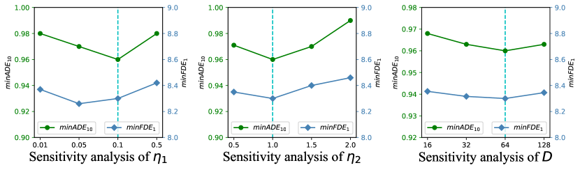
Figure S2: Ablation studies for hyper-parameters. The cyan dotted lines denote the optimum parameters.

Model	minADE5$\downarrow$	minADE10$\downarrow$	MR5$\downarrow$	MR10$\downarrow$	minFDE1$\downarrow$
w/o PE	1.41	0.98	0.63	0.41	8.35
$\mathcal{D}_{p}$	1.39	0.98	0.62	0.40	8.33
$\mathcal{S}_{p}$ (ours)	1.40	0.96	0.63	0.39	8.30
$W_{h}=W_{t}$	1.42	1.00	0.64	0.41	8.37
$W_{h}\neq W_{t}$ (ours)	1.40	0.96	0.63	0.39	8.30

Table S2: Analysis of local recursive generation. w/o PE indicates removing position embeddings. $\mathcal{D}_{p}$ denotes the dynamic learnable embeddings, while $\mathcal{S}_{p}$ denotes the static embeddings Vaswani et al. [2017]. $W_{h}=W_{t}$ denotes we use the same weight matrix for $W_{h}$ and $W_{t}$, while $W_{h}\neq W_{t}$ denotes we use the different weight matrices in Eq. (6).

B.3 Analysis of Local Recursive Generation

In this part, we analyze the sensitivity of position embeddings and weight matrices in Eq. (6) during the local recursive generation process. As shown in Table S2, either $\mathcal{D}_{p}$ or $\mathcal{S}_{p}$ contributes to performance improvements. Notably, the performance differences between $\mathcal{D}_{p}$ and $\mathcal{S}_{p}$ are minimal. Meanwhile, the performance gains achieved through position embeddings are marginal, indicating that the model obtains limited temporal information. Additionally, employing distinct weight matrices for feature projection leads to a slight performance improvement. This can be attributed to the ability of these matrices to project the head and tail steps onto the same feature space, considering their value size. Notably, our main idea revolves around the global-to-local generation process, which sets it apart from the simultaneous and recursive paradigms. During this process, as shown in Eq. (6), we propose a simple yet effective approach for achieving local recursive generation. Alternative generation methods like CVAE and diffusion models can also be employed. Generally, for these methods, it is crucial to prioritize both accuracy and efficiency.

B.4 Analysis of The Regression Loss

Model	minADE5$\downarrow$	minADE10$\downarrow$	MR5$\downarrow$	MR10$\downarrow$	minFDE1$\downarrow$
MAE	1.41	1.01	0.64	0.41	8.42
NLL	1.38	0.99	0.63	0.40	8.36
MSE (ours)	1.40	0.96	0.63	0.39	8.30

Table S3: Analysis of the regression loss. MAE indicates the Mean Absolute Error loss. MSE denotes the Mean Square Error loss. NLL denotes the Negative Log-likelihood loss. Notably, when using NLL, we utilize the Gaussian model to describe the predicted distribution. Subsequently, we utilize NLL to maximize the likelihood of the ground truths.

In this section, we investigate the sensitivity of the regression loss in Eq. (4) and Eq. (9). As shown in Table S3, our G2LTraj demonstrates robustness to these losses. These loss functions all help enforce spatial constraints among key steps. Specifically, MSE contributes the most to performance gains, while MAE performs the poorest.

B.5 Kalman Filtering for Post-processing

Model	minADE5$\downarrow$	minADE10$\downarrow$	MR5$\downarrow$	MR10$\downarrow$	minFDE1$\downarrow$
AutoBot + KF	1.45	1.09	0.69	0.45	8.73
ours	1.40	0.96	0.63	0.39	8.30

Table S4: Analysis of Kalman filter during postprocessing. KF assumes that the agents generally follow the constant velocity model as the dynamic model in Kalman filter Makansi et al. [2021].

Given that the Kalman filter can be utilized for denoising and smoothing, it raises the question of whether it can handle postprocessing kinematically infeasible predictions to generate consistent trajectories. Employing the Kalman filter requires knowledge of the dynamic motion model for agents. However, it is difficult to determine whether these agents will proceed straight, turn left, or turn right. Thus, as shown in Table S4, without the precise dynamic model for each agent, Kalman filter fails to achieve superior performance.

B.6 Visualization of The Selectable Granularity Strategy

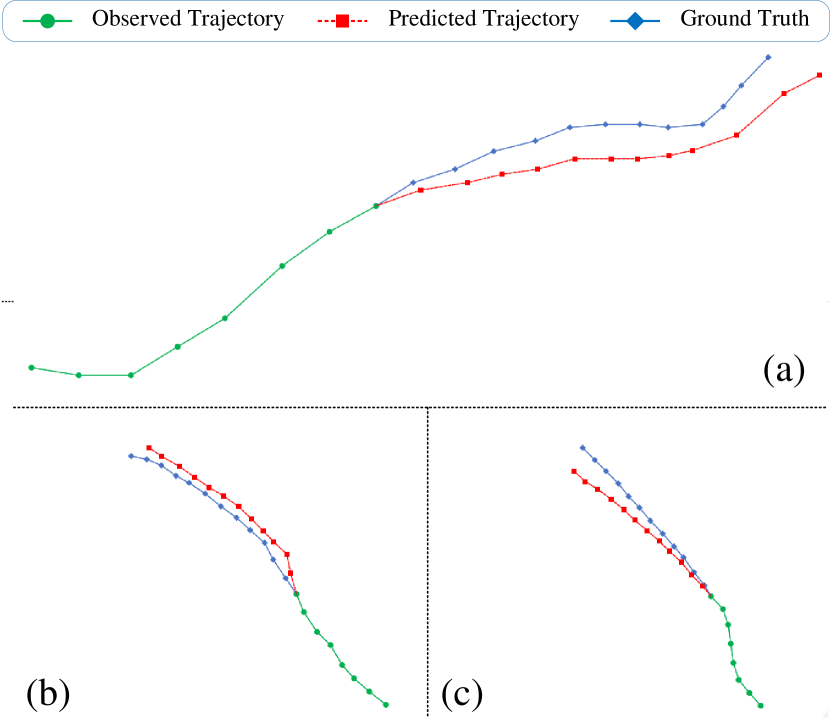
Figure S3: We enumerate three cases in the UCY validation set, and visualize their predicted most likely trajectories. The most likely trajectories for (a), (b) and (c) are generated with granularities of 2, 4, and 8, respectively.

As shown in Fig. S3, the optimal granularities vary across different agents. In particular, for Fig. S3 (a), finer granularity yields optimal trajectories by effectively capturing sudden motion changes. Conversely, for Fig. S3 (b) and (c), coarser granularities generate optimal trajectories, as the model incorporates temporal constraints from more distant steps.

References

- Alahi et al. [2016] Alexandre Alahi, Kratarth Goel, Vignesh Ramanathan, Alexandre Robicquet, Li Fei-Fei, and Silvio Savarese. Social lstm: Human trajectory prediction in crowded spaces. In Proceedings of the IEEE conference on computer vision and pattern recognition, pages 961–971, 2016.
- Aydemir et al. [2023] Görkay Aydemir, Adil Kaan Akan, and Fatma Güney. Adapt: Efficient multi-agent trajectory prediction with adaptation. In Proceedings of the IEEE/CVF International Conference on Computer Vision, pages 8295–8305, 2023.
- Bae and Jeon [2021] Inhwan Bae and Hae-Gon Jeon. Disentangled multi-relational graph convolutional network for pedestrian trajectory prediction. In Proceedings of the AAAI Conference on Artificial Intelligence, volume 35, pages 911–919, 2021.
- Bae and Jeon [2023] Inhwan Bae and Hae-Gon Jeon. A set of control points conditioned pedestrian trajectory prediction. In Proceedings of the AAAI Conference on Artificial Intelligence, volume 37, pages 6155–6165, 2023.
- Bae et al. [2023] Inhwan Bae, Jean Oh, and Hae-Gon Jeon. Eigentrajectory: Low-rank descriptors for multi-modal trajectory forecasting. In Proceedings of the IEEE/CVF International Conference on Computer Vision, pages 10017–10029, 2023.
- Caesar et al. [2020] Holger Caesar, Varun Bankiti, Alex H Lang, Sourabh Vora, Venice Erin Liong, Qiang Xu, Anush Krishnan, Yu Pan, Giancarlo Baldan, and Oscar Beijbom. nuscenes: A multimodal dataset for autonomous driving. In Proceedings of the IEEE/CVF conference on computer vision and pattern recognition, pages 11621–11631, 2020.
- Chen et al. [2021] Guangyi Chen, Junlong Li, Nuoxing Zhou, Liangliang Ren, and Jiwen Lu. Personalized trajectory prediction via distribution discrimination. In Proceedings of the IEEE/CVF International Conference on Computer Vision, pages 15580–15589, 2021.
- Girgis et al. [2022] Roger Girgis, Florian Golemo, Felipe Codevilla, Martin Weiss, Jim Aldon D’Souza, Samira Ebrahimi Kahou, Felix Heide, and Christopher Pal. Latent variable sequential set transformers for joint multi-agent motion prediction. In International Conference on Learning Representations, 2022.
- Gu et al. [2021] Junru Gu, Chen Sun, and Hang Zhao. Densetnt: End-to-end trajectory prediction from dense goal sets. In Proceedings of the IEEE/CVF International Conference on Computer Vision, pages 15303–15312, 2021.
- Gu et al. [2022] Tianpei Gu, Guangyi Chen, Junlong Li, Chunze Lin, Yongming Rao, Jie Zhou, and Jiwen Lu. Stochastic trajectory prediction via motion indeterminacy diffusion. In Proceedings of the IEEE/CVF Conference on Computer Vision and Pattern Recognition, pages 17113–17122, 2022.
- Jia et al. [2023a] Xiaosong Jia, Li Chen, Penghao Wu, Jia Zeng, Junchi Yan, Hongyang Li, and Yu Qiao. Towards capturing the temporal dynamics for trajectory prediction: a coarse-to-fine approach. In Conference on Robot Learning, pages 910–920. PMLR, 2023.
- Jia et al. [2023b] Xiaosong Jia, Penghao Wu, Li Chen, Yu Liu, Hongyang Li, and Junchi Yan. Hdgt: Heterogeneous driving graph transformer for multi-agent trajectory prediction via scene encoding. IEEE Transactions on Pattern Analysis and Machine Intelligence, 45(11):13860–13875, 2023.
- Kingma and Ba [2014] Diederik P Kingma and Jimmy Ba. Adam: A method for stochastic optimization. arXiv preprint arXiv:1412.6980, 2014.
- Lee et al. [2022] Mihee Lee, Samuel S Sohn, Seonghyeon Moon, Sejong Yoon, Mubbasir Kapadia, and Vladimir Pavlovic. Muse-vae: multi-scale vae for environment-aware long term trajectory prediction. In Proceedings of the IEEE/CVF Conference on Computer Vision and Pattern Recognition, pages 2221–2230, 2022.
- Lerner et al. [2007] Alon Lerner, Yiorgos Chrysanthou, and Dani Lischinski. Crowds by example. In Computer graphics forum, volume 26, pages 655–664. Wiley Online Library, 2007.
- Li et al. [2021] Shijie Li, Yanying Zhou, Jinhui Yi, and Juergen Gall. Spatial-temporal consistency network for low-latency trajectory forecasting. In Proceedings of the IEEE/CVF International Conference on Computer Vision, pages 1940–1949, 2021.
- Loshchilov and Hutter [2018] Ilya Loshchilov and Frank Hutter. Decoupled weight decay regularization. In International Conference on Learning Representations, 2018.
- Makansi et al. [2021] Osama Makansi, Özgün Cicek, Yassine Marrakchi, and Thomas Brox. On exposing the challenging long tail in future prediction of traffic actors. In Proceedings of the IEEE/CVF International Conference on Computer Vision, pages 13147–13157, 2021.
- Mangalam et al. [2020] Karttikeya Mangalam, Harshayu Girase, Shreyas Agarwal, Kuan-Hui Lee, Ehsan Adeli, Jitendra Malik, and Adrien Gaidon. It is not the journey but the destination: Endpoint conditioned trajectory prediction. In Computer Vision–ECCV 2020: 16th European Conference, Glasgow, UK, August 23–28, 2020, Proceedings, Part II 16, pages 759–776. Springer, 2020.
- Mangalam et al. [2021] Karttikeya Mangalam, Yang An, Harshayu Girase, and Jitendra Malik. From goals, waypoints & paths to long term human trajectory forecasting. In Proceedings of the IEEE/CVF International Conference on Computer Vision, pages 15233–15242, 2021.
- Marchetti et al. [2022] Francesco Marchetti, Federico Becattini, Lorenzo Seidenari, and Alberto Del Bimbo. Smemo: social memory for trajectory forecasting. arXiv preprint arXiv:2203.12446, 2022.
- Mohamed et al. [2020] Abduallah Mohamed, Kun Qian, Mohamed Elhoseiny, and Christian Claudel. Social-stgcnn: A social spatio-temporal graph convolutional neural network for human trajectory prediction. In Proceedings of the IEEE/CVF conference on computer vision and pattern recognition, pages 14424–14432, 2020.
- Navarro and Oh [2022] Ingrid Navarro and Jean Oh. Social-patternn: Socially-aware trajectory prediction guided by motion patterns. In 2022 IEEE/RSJ International Conference on Intelligent Robots and Systems (IROS), pages 9859–9864. IEEE, 2022.
- Pellegrini et al. [2009] Stefano Pellegrini, Andreas Ess, Konrad Schindler, and Luc Van Gool. You’ll never walk alone: Modeling social behavior for multi-target tracking. In 2009 IEEE 12th international conference on computer vision, pages 261–268. IEEE, 2009.
- Salzmann et al. [2020] Tim Salzmann, Boris Ivanovic, Punarjay Chakravarty, and Marco Pavone. Trajectron++: Dynamically-feasible trajectory forecasting with heterogeneous data. In Computer Vision–ECCV 2020: 16th European Conference, Glasgow, UK, August 23–28, 2020, Proceedings, Part XVIII 16, pages 683–700. Springer, 2020.
- Shi et al. [2021] Liushuai Shi, Le Wang, Chengjiang Long, Sanping Zhou, Mo Zhou, Zhenxing Niu, and Gang Hua. Sgcn: Sparse graph convolution network for pedestrian trajectory prediction. In Proceedings of the IEEE/CVF Conference on Computer Vision and Pattern Recognition, pages 8994–9003, 2021.
- Shi et al. [2022a] Liushuai Shi, Le Wang, Chengjiang Long, Sanping Zhou, Fang Zheng, Nanning Zheng, and Gang Hua. Social interpretable tree for pedestrian trajectory prediction. In Proceedings of the AAAI Conference on Artificial Intelligence, volume 36, pages 2235–2243, 2022.
- Shi et al. [2022b] Shaoshuai Shi, Li Jiang, Dengxin Dai, and Bernt Schiele. Motion transformer with global intention localization and local movement refinement. Advances in Neural Information Processing Systems, 35:6531–6543, 2022.
- Varadarajan et al. [2022] Balakrishnan Varadarajan, Ahmed Hefny, Avikalp Srivastava, Khaled S Refaat, Nigamaa Nayakanti, Andre Cornman, Kan Chen, Bertrand Douillard, Chi Pang Lam, Dragomir Anguelov, et al. Multipath++: Efficient information fusion and trajectory aggregation for behavior prediction. In 2022 International Conference on Robotics and Automation (ICRA), pages 7814–7821. IEEE, 2022.
- Vaswani et al. [2017] Ashish Vaswani, Noam Shazeer, Niki Parmar, Jakob Uszkoreit, Llion Jones, Aidan N Gomez, Łukasz Kaiser, and Illia Polosukhin. Attention is all you need. Advances in neural information processing systems, 30, 2017.
- Xu et al. [2020] Yi Xu, Jing Yang, and Shaoyi Du. Cf-lstm: Cascaded feature-based long short-term networks for predicting pedestrian trajectory. In Proceedings of the AAAI Conference on Artificial Intelligence, volume 34, pages 12541–12548, 2020.
- Ye et al. [2022] Maosheng Ye, Jiamiao Xu, Xunnong Xu, Tengfei Wang, Tongyi Cao, and Qifeng Chen. Dcms: Motion forecasting with dual consistency and multi-pseudo-target supervision. arXiv preprint arXiv:2204.05859, 2022.
- Yuan et al. [2021] Ye Yuan, Xinshuo Weng, Yanglan Ou, and Kris M Kitani. Agentformer: Agent-aware transformers for socio-temporal multi-agent forecasting. In Proceedings of the IEEE/CVF International Conference on Computer Vision, pages 9813–9823, 2021.
- Zeng et al. [2023] Ailing Zeng, Muxi Chen, Lei Zhang, and Qiang Xu. Are transformers effective for time series forecasting? In Proceedings of the AAAI conference on artificial intelligence, volume 37, pages 11121–11128, 2023.
- Zhao and Wildes [2021] He Zhao and Richard P Wildes. Where are you heading? dynamic trajectory prediction with expert goal examples. In Proceedings of the IEEE/CVF International Conference on Computer Vision, pages 7629–7638, 2021.
- Zhou et al. [2021] Haoyi Zhou, Shanghang Zhang, Jieqi Peng, Shuai Zhang, Jianxin Li, Hui Xiong, and Wancai Zhang. Informer: Beyond efficient transformer for long sequence time-series forecasting. In The Thirty-Fifth AAAI Conference on Artificial Intelligence, AAAI 2021, Virtual Conference, volume 35, pages 11106–11115. AAAI Press, 2021.
- Zhou et al. [2023] Zikang Zhou, Jianping Wang, Yung-Hui Li, and Yu-Kai Huang. Query-centric trajectory prediction. In Proceedings of the IEEE/CVF Conference on Computer Vision and Pattern Recognition, pages 17863–17873, 2023.