Enhancing Trust in LLM-Generated Code Summaries with Calibrated Confidence Scores

Abstract

A good summary can often be very useful during program comprehension. While a brief, fluent, and relevant summary can be helpful, it does require significant human effort to produce. Often, good summaries are unavailable in software projects, thus making maintenance more difficult. There has been a considerable body of research into automated AI-based methods, using Large Language models (LLMs), to generate summaries of code; there also has been quite a bit work on ways to measure the performance of such summarization methods, with special attention paid to how closely these AI-generated summaries resemble a summary a human might have produced. Measures such as BERTScore and BLEU have been suggested and evaluated with human-subject studies.

However, LLMs often err and generate something quite unlike what a human might say. Given an LLM-produced code summary, is there a way to gauge whether it’s likely to be sufficiently similar to a human produced summary, or not? In this paper, we study this question, as a calibration problem: given a summary from an LLM, can we compute a confidence measure, which is a good indication of whether the summary is sufficiently similar to what a human would have produced in this situation? We examine this question using several LLMs, for several languages, and in several different settings. We suggest an approach which provides well-calibrated predictions of likelihood of similarity to human summaries.

I Introduction

Summaries and comments in code help maintainers understand code. In an empirical study, Hu et al surveyed developers [1] in several major software development organizations about software summarization practices. The survey responses indicated that developers value code summaries, and, furthermore, that they would appreciate tools to automatically generate such summaries for them. Automated Code Summarization has been a very active area of research [2, 3] for quite a while. Deep neural learning, for code and natural language, has helped advance summarization performance to new highs, with the current state-of-the-art achieved via the use of in-context learning (or prompt engineering) with large language models (LLMs) [4, 5].

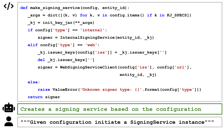
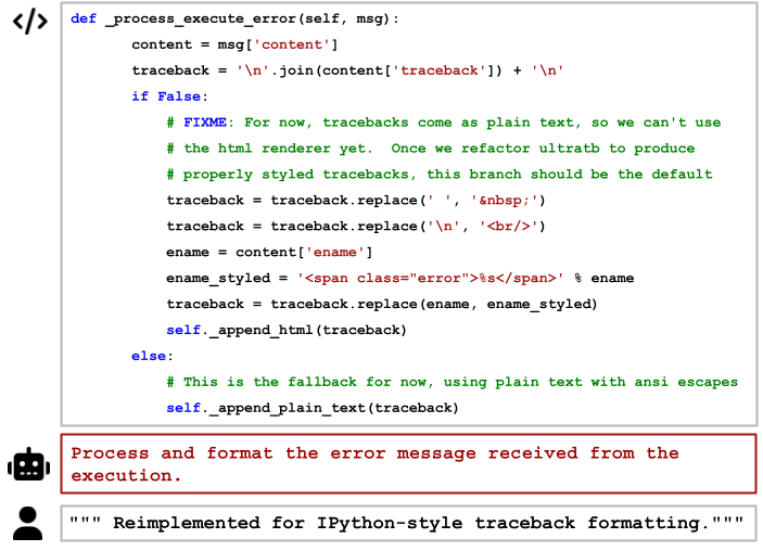
Figure 1: Example illustrating LLM-generated summaries similar (top) and dissimilar to developer-written comments (bottom)

While neural models are getting ever more effective at this important task of code summarization, there is a fundamental and well-known problem with LLMs $\ldots$ they make mistakes [6, 7, 8]. In our study, we found that state-of-the-art approaches (using CodeLlama) produce Java code summaries at acceptable accuracy levels (using measures that previous studies [9] have found to be reliable proxies of human similarity judgements) about 13% of the time. This suggests that about 87% of the time, these approaches are producing summaries that humans would not find acceptable. Figure 1 provides two example generated summaries, both prima facie, looking fluent and concise; however, one resembles the developer’s comment, and one doesn’t! Although the dissimilar summary doesn’t present any false information about the code, it omits information the method’s developer finds important to explaining the code.

So, for now, summaries provided by LLMs are sometimes good and useful, but not always. Given this situation, it is desirable for LLM-based code-summarizers to provide an indication of confidence, that a specific summary generated from code, is sufficiently similar to what a human might have produced. If this confidence measure is reliable, then a summary produced with high confidence can be accepted verbatim, and used directly to help understand the code; summaries at low confidence might be simply rejected; and summaries at a medium confidence might be considered partially useful, predicating some further examination of the code. In this paper, we study the issue of providing such a confidence measure, which is a reliable indicator of how likely a generated summary is correct, viz., sufficiently similar to a human-generated summary. We make the following contributions.

• We introduce the problem of calibration for code summarizers; we frame “correctness” of generated summaries (with motivation drawn from the literature) in terms of being sufficiently similar to human-generated summaries.

• Using several thresholds of the similarity measure SentenceBERT, corresponding to several justifiable settings of “correctness” (i.e., similarity to human-produced summaries), we examine the calibration of LLMs.

• We show how LLMs augmented with in-context learning, and using modern rescaling techniques, can provide very good calibration, for the code summarization task.

• We also find that LLMs, when instructed to reflect on the correctness of code summaries, and provide a confidence in their correctness, are not very well calibrated.

Our findings provide a way for developers to make well-justified decisions regarding the use of (sometimes inaccurate) summaries generated by LLMs.

II Background & Motivation

II-A Code Summarization

Code summarization is important for code understanding and maintenance [10]. According to Xia et al., on average, developers spend 58% of their time comprehending programs written by other people or prior code written by themselves [11]. Good quality comments can be very helpful in helping maintainers comprehenend code. Given the human effort required to construct pertinent, fluent and understandable summaries, there has been considerable interest in automated code summarization, aided by Large Language Models (LLMs).

With automated code summarization, we present a trained model with the method or code snippet as input, and we expect the model to generate a summary (similar to what might have been produced via human effort) as output. Several models have been applied to code summarization. CodeBERT [12], PLBART [13], PolyGlot [14], and CodeT5 [15] are all pre-trained language models, which have been applied to this problem. With models using pre-taining + fine-tuning, we first pre-train the models with unsupervised data in a semi-supervised way (e.g., token infilling, next token prediction) to familiarize the model with the underlying distribution of the programming language or natural language we are dealing with. We then re-train (“fine-tune”) the model with the labeled or supervised dataset in the second stage [16].

Large Language Models (LLMs) like the GPT-3 model (e.g., Code-Davinci-002) [17, 18, 5] do not require fine-tuning. With such powerful LLMs paired with in-context learning techniques e.g few-shotting [17, 18] and semantic augmentation [4], we can attain state-of-the art code summarization performance [18, 4] without expensive model training. So, in this paper, our focus is on LLM-based code summarizers that use in-context learning. Detailed methodology is explained in Section IV-C.

II-B Code Summary Evaluation

Our goal is to get LLMs to provide a code summary along with a a reliable indication of the likelihood that the summary is “good” — but what makes a summary “good”?

There has been a quite a bit of work on evaluations of code summaries [19, 20, 9, 21]. Hu et al. [1] surveyed developers at several organizations, to learn what they sought in a good code summary. The survey indicated several important criteria that automated code-summarization tools should consider: content adequacy i.e. the amount of information important to understanding the method summarized, similarity to human-produced summaries, conciseness and fluency. Among these, the importance of similiarity to human-produced summaries was separately confirmed by Stapleton et al [22]; they found human subjects performed better on tasks when they had access to a human-produced summary than a machine-generated summary.

Even prior to this important work, there has been a continuing quest for (and debates about) the right metrics [9, 19, 20, 22] to measure the similarity of a machine-generated summary to a human-produced summary. Metrics such as BLEU [23], ROGUE [24], METEOR [25] have been used to measure lexical (word n-gram level) similarity; but these have been criticized as not being well-aligned to human judgements of similarity in the case of code summaries [22]. Haque et al. [9] empirically compared 10 different lexical & semantic metrics of similarity, and found that certain embedding-based metrics such as SentenceBERT are better-correlated with human evaluations of summary similarity (to a reference) than purely lexical measures. They report that SentenceBERT has the highest correlation with human evaluations of summary similarity.

Besides similarity to human-produced summary, another important criterion is content adequacy: is the summary a useful, relevant summary of the code? Recently, Mastropaolo et al. [21] introduced SIDE, a way to automatically measure content adequacy of a candidate summary using just the code and the candidate summary (and no reference). They develop an ordered logistic regression model using only automatic metrics as independent variables, to predict human evaluations of content adequacy. They find that SIDE, SentenceBERT, and other metrics are complementary — all are useful predictors of content adequacy and carry orthogonal information to each other. They find that metrics for similarity to code are the most significant predictors, particularly SIDE.

Thus, we have a strong predictive metric for content adequacy from Mastropaolo et al. It is also possible for a reader to judge the fluency and conciseness directly from the generated summary. Moreover, prior work indicates the importance of similarity to human-produced summaries [22]; Consequently, we focus our study on predicting similarity to human-produced summaries without access to a human-produced reference.

II-C Calibration

Calibration is the property of providing an accurate indication of confidence in a predictive system. Calibration relates to the reliability of a model’s confidence in its output. For instance, consider a weather model predicting a 60% confidence (probability) of rain for the next day. If this model is run over several years and it rains just about 60% of the days when it forecasts with 60% confidence, we deem it well-calibrated. In such a case, the model’s confidence level closely aligns with the actual frequency of correct predictions, indicating its reliability.

A well-calibrated model allows rational decision-making. In weather forecasting, a well-calibrated model enables users to respond appropriately across a spectrum of confidence levels: for instance, carrying a hat at 10% confidence of rain, carrying an umbrella at probabilities 50% or above, or opting for enclosed vehicular transport at 80% or above. The concept of calibration has recently gained significance in the field of natural language processing.

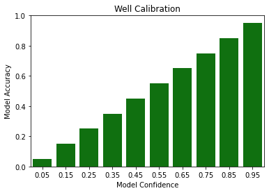
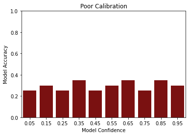
Figure 2: Example illustrating well and poorly calibrated models

Calibration is a relationship ( Figure 2) between two quantities: confidence on the x-axis, typically a probability value, and the rate of correctness (y-axis), typically a normalized frequency (values $\in[0,1]$) indicating how often the model is empirically correct, when predicting at the confidence values along the x-axis. Figure 2 presents two reliability plots [26] to show the difference between a well-calibrated model and a poorly calibrated model; in the plot, the predicted confidences are binned along the x-axis, over 10 ranges $0-0.1,0.1-0.2,\ldots$, and the fraction of each bin that is correctly predicted is shown on the y-axis. In a well-calibrated model, the observed model correctness rate is well-aligned with the model confidence; for a poorly calibrated model, it is not. Well-calibrated models provide a confidence that is a good indicator of likely correctness, which can be used for rational decision-making.

II-D Calibration for Code Summarization

Unfortunately, the notion of calibration in generative settings is complicated. In classification settings, calibration is a straightforward concept, because obtaining model confidence (from the softmax layer) for a specific predicted class or solution is straightforward, and correctness in classification is typically measured using binary values (1 for correct and 0 for incorrect). This is not so straightforward for generative tasks like code summarization; several complications arise.

First, there are several different ways to measure a model’s confidence. A generative model produces a confidence per token it generates; one needs to summarize these confidences across the entire generated sequence. In addition, with an instruction-tuned model of sufficient power, one can also prompt the model again, with the code and the summary it generated, to provide its confidence in its own output.

Second, the results obtained from automatic metrics (e.g., BLEU-4, SentenceBERT) are continuous, real values – making it necessary to determine when to consider the model’s output as good versus bad in the binary sense. Therefore, measuring model accuracy in the same way as in classification problems is not feasible.

In this paper, we primarily address these issues. We propose a method to compute model performance suitable in a calibration context and suggest several approaches to measure model confidence. Finally, we present a few different design choices in using the SentenceBERT metric to determine “correctness”, viz., in our case sufficient simlarity to a human-generated summary. These choices for confidence and correctness provide a range of possibilities for evaluating calibration, which we discuss further below.

III Research Questions

In this section, we will briefly discuss the research questions. In the first research question, we study whether an LLM’s confidence in its generated summary can be used to predict the quality of its generated summary. As previously established, we evaluate summary quality using metrics measuring similarity to human-produced summaries. We explore whether an LLM’s log-probabilities can be used to directly predict continuous similarity metrics. To improve prediction performance, we additionally transform the continuous prediction task to a binary one using thresholding. Instead of predicting how similar a model-generated summary is to a human one, we predict whether a generated summary is sufficiently similar to a human one. We determine multiple thresholds on similarity metrics that separate a human-like summary from a not-so human summary. Then, we study the calibration of LLMs with respect to this binary notion of summary correctness. We will discuss thresholding further in Section IV-E and present our findings in Section V-A.

Rescaling is a method used to adjust a model’s confidences to better align with the observed frequencies of events. There are several rescaling strategies, including Platt scaling [27], temperature scaling [21], isotonic regression [28], and histogram binning [29]. Platt scaling is a widely used method for improving model calibration. In this paper, we only apply Platt rescaling due to its effectiveness. In this research question, we will explore whether calibration can be improved using rescaling. Additionally, we will investigate whether prompting methods like semantic augmentation affect rescaled calibration. Furthermore, we will examine how rescaled calibration performs at multiple, useful thresholds (e.g., at high precision, high recall points). We will discuss rescaling further in Section IV-H and present our findings in Section V-B.

In the first two research questions, we measured a LLM’s confidence using its own calculated probability. In this next research question, we measure a model’s confidence by asking it to evaluate its own generated output and using this output to compute self-reflective confidence measures. In Section IV-F, we discuss these self-reflective measures and prompting techniques in detail.

These questions taken together, constitute, to our knowledge, the first detailed examination of the calibration of LLMs with respect to the code summarization task.

IV Dataset & Methodology

IV-A Dataset

In this section, we will discuss the datasets utilized in this work.

Dataset for Calibration Experiments. We use the Java and Python code summarization datasets from the CodeXGLUE [30] Benchmark for our calibration studies. CodeXGLUE includes 14 datasets covering 10 Software Engineering tasks. Java and Python datasets contain 164,923 and 251,820 training samples, respectively. We use BM25 [31] algorithms to retrieve relevant samples from these datasets for few-shotting. For the test set, we randomly select 5000 samples from each language.

Dataset for Human Evaluation Our notion of correctness is sufficient similiarity to human-produced (reference) summaries. For this, we use the Haque et al. [9] dataset, which includes reference and generated summaries for 210 Java methods. For each Java method, it includes 3 human-assigned similarity ratings. Human raters select from 4 ratings ranging from ”Strongly Disagree” to ”Strongly Agree” indicating their agreement that the generated summary is similar to the reference. Following their methodology, for each code method, we take the mean of the 3 human ratings to produce an aggregate, representative rating. We use this dataset to evaluate how accurately different automatic similarity metrics classify human agreement vs. disagreement on a summary’s similarity to the reference. In Table II, we present the AUC-ROC values for various similarity metrics. In Section V-A, we discuss the necessity of AUC-ROC and the method for selecting the most appropriate automatic similarity metric.

IV-B Models

In this section, we will briefly discuss the three models we used for the experiments.

GPT-3.5-Turbo. GPT-3.5 models perform well at both comprehension and generation, for both natural language and code [32]. GPT-3.5-Turbo is the most capable and affordable option among these models. Although it is primarily optimized for chat-based interactions, it also performs well in non-chat tasks. For our research, GPT-3.5-Turbo can generate up to 16,385 tokens, including the prompt tokens.

Code-Llama-70b. Code Llama [33], a family of large language models tailored for coding tasks, builds upon Llama 2’s [34] architecture, showcasing leading performance among open models. It boasts infilling capabilities, support for extensive input contexts, and zero-shot instruction-following abilities. The family includes foundation models, Python-specialized variants, and instruction-following models, each with 7B, 13B, 34B, and 70B parameters. Trained on 16k-token sequences, these models excel on inputs of up to 100k tokens. Notably, Code Llama achieves state-of-the-art results on various code benchmarks. Since larger models yield better performance, we use just the 70B parameter model for our experiments.

DeepSeek-Coder-33b Instruct. The DeepSeek-Coder series introduces open-source code models ranging from 1.3B to 33B parameters, trained from scratch on a massive 2 trillion-token dataset [32]. These models, pre-trained on high-quality project-level code corpora, utilize a fill-in-the-blank task with a 16K window to enhance code generation and infilling. Extensive evaluations demonstrate that DeepSeek-Coder achieves state-of-the-art performance among open-source code models across various benchmarks, outperforming closed-source models like Codex and GPT-3.5. We use the 33B paramater model for our study.

IV-C Prompting Methods for Code Summaries

In this section, we describe our two approaches to in-context learning (viz., prompting).

Retrieval Augmented Few-shot Learning. Few-shot learning works well for both Natural Language Processing [17] and Software Engineering [18, 5]. In few-shot learning, we present the models with a few exemplars as query-answer pairs (method-comment pairs in this setup) and instruct the model to answer our final query (only the method).

Several works show that the model performance with few-shot learning can be improved using relevant samples, which can be extracted using the BM25 algorithm [4, 5]. Since Retrieval Augmented Few-shot learning is known to work better than vanilla few-shot learning for many SE tasks (e.g., code summarization, program repair, and assertion generation), we focus only on BM25 augmented few-shot learning.

Automatic Semantic Augmentation of Prompt (ASAP). Chain-of-thought [35] has been found to be effective for several tasks in NLP: providing the model with examples comprising explicit intermediate reasoning steps improves performance. For SE, Ahmed et al., showed a workable approach to extracting such “intermediate steps” using static analysis algorithms; this approach enhances model performance [4]. They used GitHub repository information, identifier type with scope, and dataflow information. Combined with BM25, this approach yielded state-of-the-art performance for code summarization tasks. We also applied this approach to the problem and observed how calibration changes with it.

IV-D Evaluating similarity to human-produced summaries

In Section II-B we described the range of available metrics, and justified our focus on measures of the similarity to human-produced summaries. Following Haque et al. we focused on semantic measures of similarity, although we did a preliminary screening of 7 different measures, including both lexical and semantic measures.

In the semantic categoery, we used Infersent-CS [36], SentenceBERT-CS [37], BERTScore-CS [38], and SIDE [21] for our experiment. Among these, we have found that SentenceBERT-CS is the most effective metric.

For a notion of correctness, viz., “sufficient similarity”, we used thresholds.

IV-E Thresholding Summary Quality Metrics

Our notion of correctness is sufficient similarity to human-produced summaries; this requires thresholding similarity metrics, which are real numbers. Using data from existing human studies, we determine multiple reasonable thresholds on similarity metrics that separate a human-like summary from a not-so human summary. This allows users to select different thresholds, based on their situation. For example, a cautious developer may want only those summaries most similar to human-written summaries; a less cautious person might want some reasonable summary, even if lacking assurance of similarity to human summaries. For our purposes here, we would like to evaluate calibration in regards to different thresholds.

The AUC-ROC measure assesses binary classification models by calculating the area under their Receiver Operating Characteristic curve, which measures their ability to distinguish between positive and negative classes across various thresholds. It yields a single scalar value for easy performance comparison, remains robust against class imbalance, and provides valuable insights into a model’s discrimination capability, enhancing its utility for evaluating and comparing binary classifiers. The AUC-ROC value ranges from 0 to 1. A value of 0 indicates that the model’s predictions are entirely incorrect, while a value of 1 indicates perfect predictions. Usually, AUC-ROC values range between 0.5 to 1.0 because random assignment of binary classes can yield a AUC-ROC of 0.5.

As mentioned earlier, the evaluation metrics for code summarization are continuous, and calibration can only be evaluated for classification tasks. We can select the threshold that gives the best F1-score and use that to convert the continuous value to a binary value. For example, if the score from a similarity metric (e.g., SentenceBERT) is higher than a certain value (e.g., 0.80), we consider the solution good; otherwise, it is considered bad. We can vary this threshold, and evaluate calibration at different thresholds, to evaluate the capability and flexibity of our calibration approach.

IV-F How to measure models’ confidence?

In this section, we will briefly discuss the methods we used for measuring model confidence.

Average Token Probability. In this paper, we use one intrinsic measure to calculate the model confidence: average token probability. To compute average token probability, we gather the auto-regressive token probabilities of the tokens generated by the model and calculate their arithmetic mean – producing a probability over the entire generated sequence. Obtaining model confidence with a classification model is much simpler, because each class is assigned one probability [39, 40]. However, for a generative task, each token comes with an individual probability. We find that average token probability is empirically a good measure of the model’s confidence.

Self-reflective Measure. By “reflective measure” we denote measures obtained by prompting an instruction-tuned model to evaluate it’s own output. We used two reflective measures to compute model confidence. One is logit-based, and the other one is verbalized. In the logit-based measure, we present the model with the code and model-generated summary, and ask the model about the quality of the summary using a true/false method (see Figure 9 for the prompt). We review the top five tokens, by their probabilities, and select the probability associated with the “True” token. For the verbalized measure, we tried both zero-shot and few-shot learning approaches and asked the model to assign a score from 1 to 4 based on similarity, following the approach used by Haque et al. [9]’s tool for human validation. Figure 8 presents the prompt for the verbalized confidence measure.

IV-G Measures of Calibration

A calibration metric measures the alighnment of a model’s confidence (in its predictions) with the correctness thereof. The plots in  Figure 2 shows how a model’s confidence in its output can be (or not) very well-aligned the correctness of the output. There are several measures of the degree of this alignment, which we now discuss.

Brier. The Brier Score [41] measure of calibration is calculated as the mean squared difference between the predicted probabilities and the actual outcomes. In the context of calibration, the Brier Score assesses how well the predicted probabilities align with the actual frequencies of events. A perfectly calibrated model would have a Brier Score of 0, indicating that its predicted probabilities match the observed frequencies exactly. Mathematically, the Brier Score is calculated as follows:

$$B_{r}=\frac{1}{N}\sum_{i=1}^{N}(\hat{p_{i}}-\hat{o_{i}})^{2}$$ (1)

$B_{r}$ represents the Brier Score, $N$ is the total number of samples, $\hat{p_{i}}$ is the probability assigned to the $i^{th}$ sample prediction, and $\hat{o_{i}}$ is the prediction outcome (1 for correct, 0 for incorrect) for the $i^{th}$ sample. Lower Brier Scores indicate better calibration, with 0 being perfect calibration. Conversely, a higher Brier Score indicates worse calibration, with a maximum possible score of 1. Thus, the Brier Score measures the alignment of a model’s confidence estimates with the actual rate of its empirical correctness.

It should be noted, however, Brier scores are influenced by the base rate. A naïve model, that always outputs the base rate $p$, will achieve a score called the reference Brier score, $B_{ref}$, which analytically is $p(1-p)$. For example, in a 2-class prediction problem (e.g., rain/no rain), if it rains about 10% of the days, the base rate is $0.1$; a model that always outputs $0.1$ as its confidence will score $0.1*0.9=0.09$ Brier. It’s easy to see that $B_{ref}\in(0,0.25]$.

Given the possibility of low Brier scores from actually very “unskilled” naïve models, we need to normalize the measured Brier for a given model; we discuss this below, as “skill scores”.

ECE. (Expected Calibration Error) [42] is another metric used to evaluate the calibration performance. It measures the average difference between the predicted and actual probabilities across different confidence levels. Instead of focusing on specific threshold points, ECE provides a holistic view of calibration performance. A lower ECE indicates better calibration, meaning the predicted probabilities closely match the actual probabilities. Conversely, a higher ECE indicates poorer calibration, indicating a mismatch between expected and actual probabilities.

To compute Expected Calibration Error (ECE), we partition the dataset into $n$ bins $B_{i},i=1\ldots n$ based on confidences (predicted probabilities). For instance, the bins could range from [0-0.1) to [0.9-1.0), each representing different confidence levels. Next, we calculate the average confidence, $conf(B_{i})$ (predicted probability), and empirical accuracy, $acc(B_{i})$ (proportion of true positives), for each bin. Following this, we determined a weighted difference by (i) computing the absolute difference between the average confidence and accuracy in each bin and (ii) weighting by the proportion of samples in each bin. Finally, we sum the weighted differences across all bins to get the ECE. ECE provides a more nuanced evaluation of calibration across different confidence levels compared to metrics like the Brier Score, which aggregates errors across all samples without considering confidence levels. This makes ECE particularly useful for understanding how well a model’s confidence estimates align with its performance at different confidence levels. Mathematically, the ECE is calculated in three steps below (Note: $B_{i}$ denotes the set of elements in each bin; $\hat{o_{i}}$ is an indicator varible, $=1$ if the prediction is right, and $=0$ if wrong; $\hat{p_{i}}$ is the confidence (probability) associated with the prediction)

$$acc(B_{i})=\frac{1}{|B_{i}|}\sum_{\hat{o_{i}}\in B_{i}}{\hat{o_{i}}}$$ (2)

$$conf(B_{i})=\frac{1}{|B_{i}|}\sum_{\hat{p_{i}}\in B_{i}}{\hat{p_{i}}}$$ (3)

$$ECE=\displaystyle\sum_{i=1}^{m}\frac{\mid B_{i}\mid}{\mid T\mid}\lvert\text{acc}(B_{i})-\text{conf}(B_{i})\rvert$$ (4)

While ECE is intuitive, and visually appealing: it can be misleading. For example, if it almost always rains 10 days a year in Los Angeles, a naive (technically, “unskilled”) model might always predict rain with a probability of $\frac{10}{365}=0.0275$. Such a model would have a single bin with a confidence of $0.0275$, and an empirically correctness rate of nearly the same (on a yearly basis), yielding a perfect (but misleading) ECE of zero.

To avoid this issue, and to properly characterize a model’s skill beyond simple base-rate naïveté, we use the Brier Skill score.

		BERT Score	BLEU-1	Infersent-CS	ROUGE-1-P	ROUGE-4-R	ROUGE-W-R	Sentence BERT
Language	Model
Java	CodeLlama-70b-hf	0.31	0.25	0.26	0.26	0.37	0.17	0.26
	deepseek-coder-33b-instruct	0.32	0.21	0.30	0.28	0.36	0.24	0.28
	gpt-3.5-turbo	0.24	0.14	0.24	0.27	0.30	0.03	0.20
Python	CodeLlama-70b-hf	0.45	0.41	0.44	0.45	0.45	0.33	0.43
	deepseek-coder-33b-instruct	0.33	0.25	0.30	0.34	0.34	0.25	0.31
	gpt-3.5-turbo	0.17	0.07	0.15	0.21	0.18	0.13	0.17

TABLE I: Spearman Rank Correlation between Average Token Probability and Summary Evaluation Metrics

Brier Skill Score. A “skill score” is a normalized measure $\in(-\infty,1]$ for assessing the reliability of a model’s confidence, beyond just always providing the base rate as the confidence.

As discussed earlier, a naïve model always outputting the base rate as its confidence reaches the $B_{ref}$ Brier score of $p(1-p)$, which can be quite low, depending on $p$. One can do better than $B_{ref}$ with good models. For a two-class prediction, with a 50% overall positive rate: a naive predictor randomly guessing always guessing one class with 10% confidence yields $B_{ref}\approx 0.09$. However, with well-calibrated confidences, a skilled model can achieve a Brier Score lower than this unskilled $B_{ref}$ value. Of course, with a bad model, one can do worse! The Skill Score (SS) quantifies this improvement (or decline) compared to the baseline $B_{ref}$, calculated as:

$$SS=\frac{(B_{ref}-B_{model})}{B_{ref}}$$ (5)

A positive SS (perfect score = 1.0) indicates improvement over the baseline, while a negative SS suggests predictions worse than the baseline. Small positive values of SS can sometimes indicate good skill. The German weather forecasting service, Deutsche Wetterdienst, sets a minimum threshold of 0.05 for a Skill Score to indicate good forecast quality reference [43]. Another reference point comes from the American data journalism site 538, which reports a skill score of approximately 0.13 in forecasting World Cup games [44] Both ECE and Brier Score serve slightly different purposes: the Brier Score measures the ability to correctly discriminate output categories and the calibration of output probability for each sample, while the ECE specifically measures calibration. However, the ECE can be misleadingly low, as noted earlier for the unskilled predictor. Additionally, careful binning is necessary as it can impact ECE scores.

IV-H Rescaling

Rescaling involves adjusting the predicted probabilities of a model to better align with the observed frequencies of events. Platt Scaling [27] is a commonly employed method in calibration, where a logistic regression model is fitted to the predicted probabilities alongside the corresponding true outcomes. Through this process, the model fine-tunes the predicted probabilities to more accurately reflect the true probabilities of events. Other rescaling approaches include temperature scaling [39], isotonic regression [28], and histogram binning [29]. In this paper, we restrict ourselves to Platt Scaling, which is a widely used approach that proved effective for our task. For Platt scaling, we employ 5-fold cross-validation, where for each fold, we utilize the other 4 folds as training data and apply the learned regression to our target fold. We repeat this process for all other folds to obtain rescaled values for all samples. To accurately evaluate that rescaling is robust, we construct our folds such that each fold contains samples from different sets of repositories. This way, our test set is always pulled from different repositories than our training set.

V Result

V-A RQ1 Calibration: LLM Confidence vs. Summary Correctness

Metric	AUC ROC
ROUGE-1-P	0.869
ROUGE-4-R	0.837
ROUGE-W-R	0.825
BLEU-1	0.862
Infersent-CS	0.839
SentenceBert-CS	0.903
BERT Score-R	0.864

TABLE II: Thresholding Metric Performance

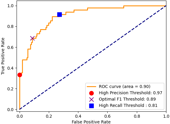
Figure 3: SentenceBERT ROC Curve

To begin with, one might wonder if the per-token probabilities produced by a LLM are directly good predictors of similarity to a human summary? If this were the case, the developer could get an accurate sense of similarity through these probabilities. In Table I, we present the Spearman Rank Correlation between the average token probability and computed evaluation metrics on LLM-generated summaries. For Code-Llama-70B, the rank correlation ranges between 0.17 and 0.45 across 2 programming languages and 7 evaluation metrics. For GPT-3.5-Turbo, the rank correlations are significantly lower, ranging between 0.03 and 0.30. Across all configurations, the rank correlation is lower than 0.50. Although the evaluation metrics tend to increase with average token probability, the monotonic relationship is too weak to use average token probability as a direct indicator of similarity strength.

As mentioned earlier (Section V-A), we evaluate AUC-ROC for different metrics, with respect to human judgements of similarity. Through the Haque et al. [9] dataset, we have human ratings for similarity of generated summaries, with the (included) reference summary. Using the reference and generated summaries, we can readily calculate the automated similarity metrics. To qualify as a positive sample, the average human rating must indicate at least “Agree”. Table II presents the AUC-ROC for each similarity metric. We observe that the AUC-ROC for all metrics is above 0.80, but the best performance is achieved with SentenceBERT. Figure  3 presents the ROC curve of SentenceBERT, displaying strong classification performance across multiple thresholds a user may desire viz high precision, high recall, and optimal F1.

SentenceBERT being a strong binary classifier of human judgement is consistent with previous work on SentenceBERT being highly correlated with human judgement[9]. However, although related, note that these results are distinct. Unlike AUC-ROC, high rank correlation implies a strong monotonic relationship, but does not consider the specific distribution of each variable in relation to multiple classification thresholds. Due to its effectiveness, moving forward, we primarily focus on Sentence BERT in our calibration study on similarity metrics.

We now present calibration results for summaries generated using few-shots retrieved by BM25. Table III, Figure 4(a) and 4(b) show the optimal F1 thresholded, raw calibration for the SentenceBERT metric. Both the Brier score and ECE are quite high. Additionally, we observed a negative skill score for all cases. The Brier score ranges from 0.30 to 0.61, which are rather bad, indicating performance worse than random assignment. For the CodeLlama-70b model, the model’s success rate is good for both Java (24%) and Python (21%). However, while these numbers are bad, there is clearly some signal in the reliablity diagrams.

		Success Rate	ECE	Brier	Skill score
Language	Model
Java	CodeLlama-70b-hf	0.13	0.50	0.34	-2.11
	deepseek-coder-33b-instruct	0.10	0.52	0.35	-2.82
	gpt-3.5-turbo	0.05	0.67	0.50	-10.05
Python	CodeLlama-70b-hf	0.09	0.50	0.32	-3.01
	deepseek-coder-33b-instruct	0.07	0.53	0.34	-4.32
	gpt-3.5-turbo	0.04	0.80	0.67	-18.96

TABLE III: Raw Calibration Metrics. “Success rate” indicates the fraction of output above similarity threshold

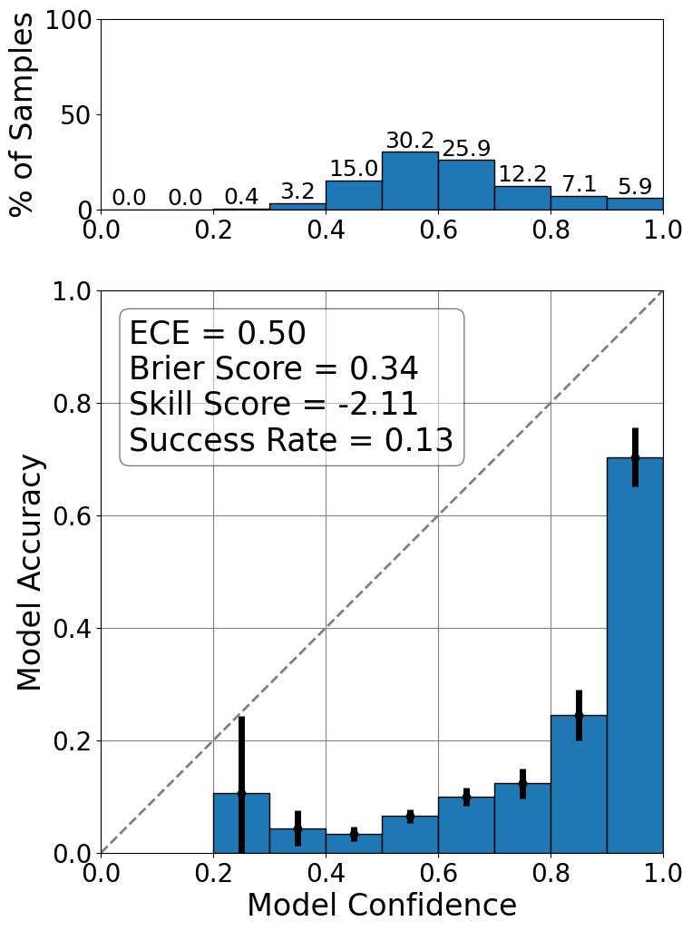
(a) Code Llama 70b

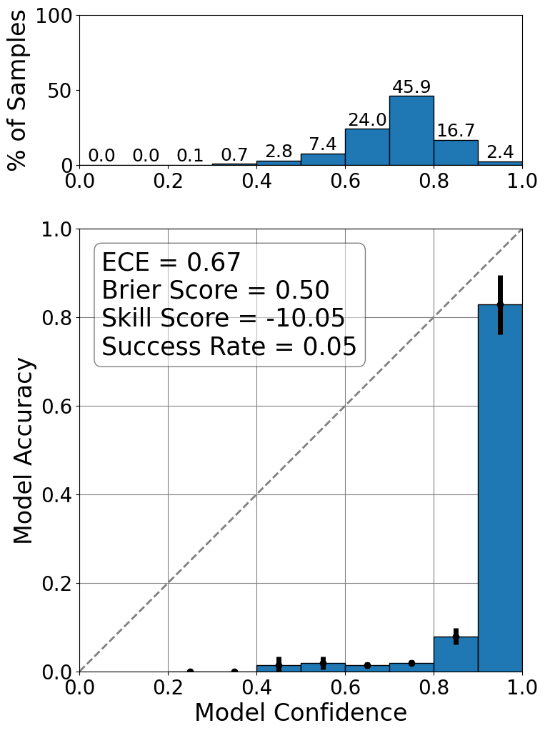
(b) GPT-3.5 Turbo

Figure 4: Reliability Plots for models using Retrieval Augmented Few-Shot Summarization on Java methods. The top plots show the frequency distribution of confidence values; the bottom is a reliability diagram.

		Success Rate	ECE	Brier	Skill score
Language	Model
Java	CodeLlama-70b	0.13	0.02	0.09	0.20
	deepseek-coder-33b-instruct	0.10	0.01	0.07	0.24
	gpt-3.5-turbo	0.05	0.01	0.04	0.20
Python	CodeLlama-70b	0.09	0.01	0.07	0.19
	deepseek-coder-33b-instruct	0.07	0.00	0.05	0.14
	gpt-3.5-turbo	0.04	0.00	0.03	0.05

TABLE IV: Platt Rescaled Calibration using Retrieval Augmented Few-Shot Summarization on Java methods

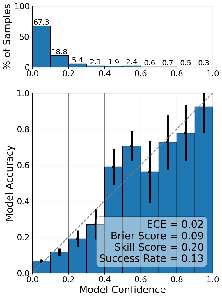
(a) Code Llama 70b

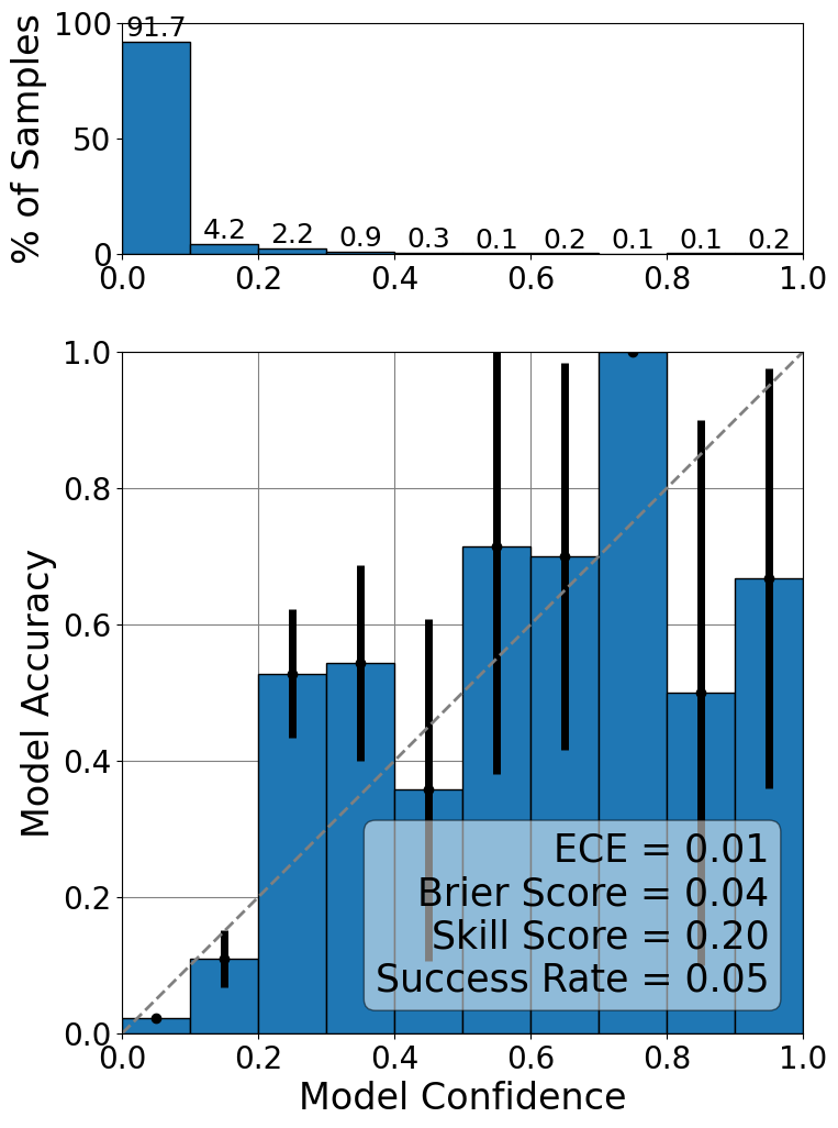
(b) GPT-3.5 Turbo

Figure 5: Rescaled Reliability Plots (of Figure 4). Note that the rescaled blue bars are closer to the diagonal, and the distribution of confidence values changes (top plots) as confidence values are scaled

		Success Rate	ECE	Brier	Skill score
Language	Model
Java	CodeLlama-70b	0.14	0.01	0.11	0.13
	deepseek-coder-33b-instruct	0.11	0.01	0.08	0.20
	gpt-3.5-turbo	0.09	0.03	0.07	0.17
Python	CodeLlama-70b	0.13	0.01	0.09	0.24
	deepseek-coder-33b-instruct	0.09	0.01	0.07	0.15
	gpt-3.5-turbo	0.03	0.00	0.03	0.01

TABLE V: Platt Rescaled Calibration using Automatic Semantic Augmentation + Retrieval Augmented Few-Shot for summarization of Java methods

		Success Rate		Brier		ECE		Skill score
	Threshold Type	High P	High R	High P	High R	High P	High R	High P	High R
Language	Model
Java	CodeLlama-70b	0.06	0.22	0.04	0.15	0.01	0.02	0.36	0.10
	deepseek-coder-33b-instruct	0.05	0.19	0.03	0.14	0.01	0.02	0.46	0.13
	gpt-3.5-turbo	0.03	0.12	0.02	0.09	0.01	0.02	0.29	0.07
Python	CodeLlama-70b	0.04	0.18	0.03	0.13	0.00	0.02	0.26	0.11
	deepseek-coder-33b-instruct	0.03	0.16	0.02	0.12	0.00	0.01	0.27	0.08
	gpt-3.5-turbo	0.01	0.10	0.01	0.09	0.00	0.01	0.04	0.03

TABLE VI: Calibration under high precision and recall thresholds

V-B RQ2: Platt Rescaled vs. Raw Calibration

We now study how calibration changes with rescaling. Table IV and Figure 5 show Brier scores, ECE, and skill scores at different setups. Following the prior research question, we use the intrinsic measure of average token probability to calculate model confidence. We have very high skill (0.20+) for Java on each model. With CodeLlama-70b, we have a very high skill score for Python (0.19), and for other models, we also have very strong/strong skill scores for Python (0.14 & 0.05). The Brier scores now range from 0.03 to 0.09, which are quite low, indicating that the models are well calibrated. We also observe that the ECE greatly reduces with rescaling. To summarize, the thresholded raw average token probability is not well-calibrated, but the thresholded rescaled average token probability is well-calibrated. Therefore, the reliability of the model increases with rescaling.

Calibration changes with ASAP. Table V presents the results comparing calibration applying ASAP. We observe that, augmented with static analysis products, more of the model’s output exceeds the threshold (higher success rate) in all cases except for Python with the GPT-3 Turbo model.

Turning now to the calibration, for Java, the skill score decreases with ASAP, whereas for Python, the skill score increases for the CodeLlama-70B and deepseek-coder-33b-instruct models. In these two cases, the skill score increases alongside success rate. It’s noteworthy that Java is a strictly typed and verbose language; the additional information provided by ASAP in the prompts may be redundant, and distort the model’s confidence. However, for Python, ASAP may provide necessary information that might be missing in the function body itself (e.g., variable type). Incorporating this information may be helping improve both success rate and calibration. Hence, the trade-off exists, at least for Java, where transitioning from BM25 to ASAP yields better performance but less reliability.

Calibration effects of thresholding So far, we have calculated the skill score thresholded at optimal F1-score. What about other threshold points, e.g., for high precision points and high recall? Note that we achieve high precision at very high thresholds and high recall at low thresholds. As expected, at high thresholds, the model’s rate of success is very low. At high recall points, the success rate will be higher. Similar to our experimental trend, we can observe that the low success rate models are more reliable with high skill scores. The skill score at high precision point thresholding is 0.20+ except for Python with the GPT-3.5-turbo model. On the other hand, the skill score at high recall points ranges from 0.03 to 0.13. Thus, the usage of thresholds should be managed with care, as both success rate and skill score are influenced by it.

		Success Rate	ECE	Brier	Skill score
Language
Java	Raw	0.09	0.88	0.86	-9.4
	Rescaled	0.09	0.02	0.08	-0.01
Python	Raw	0.04	0.90	0.86	-21.89
	Rescaled	0.04	0.00	0.04	-0.00

TABLE VII: GPT-3.5-Turbo Reflective Logit Calibration

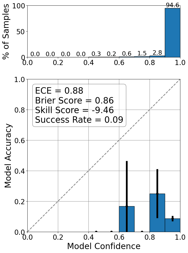
(a) Reliability Plot

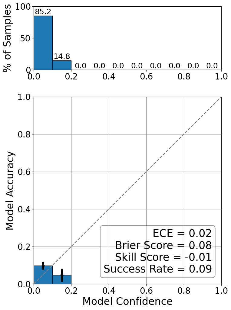
(b) Rescaled Reliability Plot

Figure 6: GPT-3.5-Turbo Reflective Logit Reliability Plots for Java

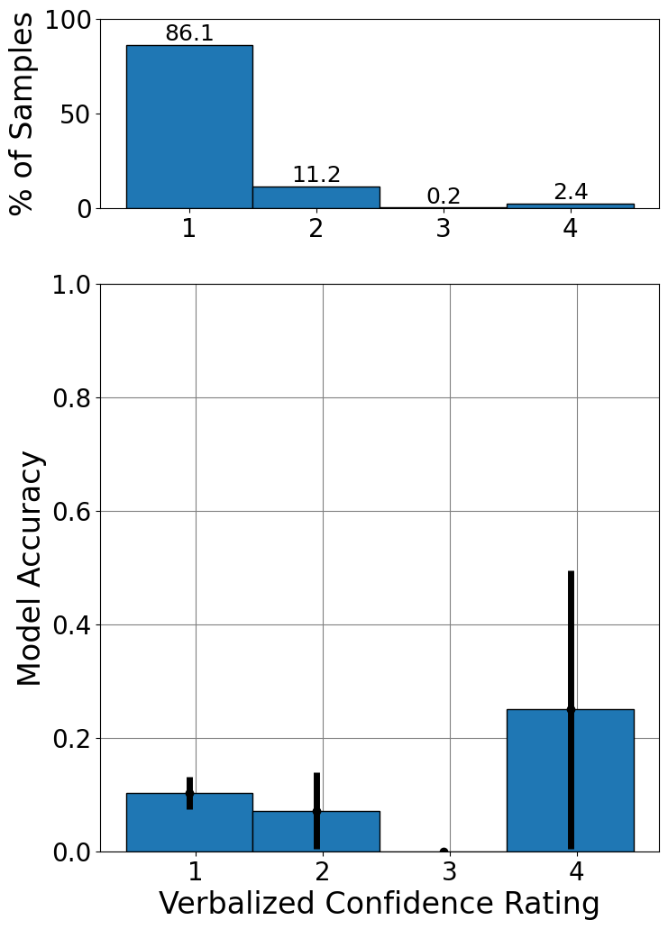
(a) deepseek-coder-33b-instruct Java

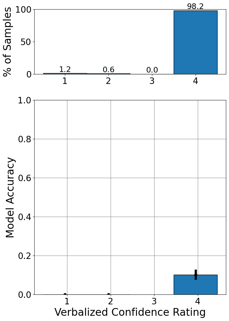
(b) GPT-3.5 Turbo on Java

Figure 7: 0-shot Verbalized Confidence

V-C RQ3: Self-Reflection Calibration

In Section IV-F, we discussed multiple methods to measure self-reflective model confidence. In regards to the reflective logit, when we prompt the model to generate true/false responses (see Figure 9), CodeLlama-70b produced invalid responses on extensive prompt variations since it is not instruction-tuned. Additionally, we are interested in the logit associated with the token “True”. If the model does not generate “True”, it is impossible to retrieve the “True” logit unless we have access to the top-k log-probability tokens and “True” is one of them. Among our models, we only have this access for GPT-3.5-Turbo due to API limitations (see  VI-A). Consequently, we only evaluated reflective logits on the GPT-3.5-Turbo model. However, the model was highly over-confident with 94% of its confidences over 0.9, achieving a negative skill score (see Figure 6 and Table VII). Rescaling transformed all the logits to near the unskilled, base rate.

We also attempted zero-shot and few-shot verbalized confidence measures by prompting the model to assign either 1, 2, 3, or 4 to score the similarity between the reference and the generated output (see Figure 8 for the prompt).

This design choice is inspired by human evaluations by Haque et al. [9]. In this setup, CodeLlama-70b failed to generate any score, but in the few-shot learning scenario, CodeLlama-70b is able to generate scores. During few-shot learning, the shots were taken from the dataset proposed by Haque et al. Figure 7 presents calibration with the 0-shot verbalized confidence. In the x-axis, we present the verbalized confidence scores, and on the y-axis is accuracy with respect to optimal F1 thresholded Sentence-BERT. For both zero-shot and few-shot settings, we found that the models were similarly not well-calibrated. Note that we tried a higher temperature and generated multiple samples. Majority voting from multiple samples did not change the calibration outcome.

Therefore, we can conclude that the models are not well-calibrated for any of the self-reflective measures studied.

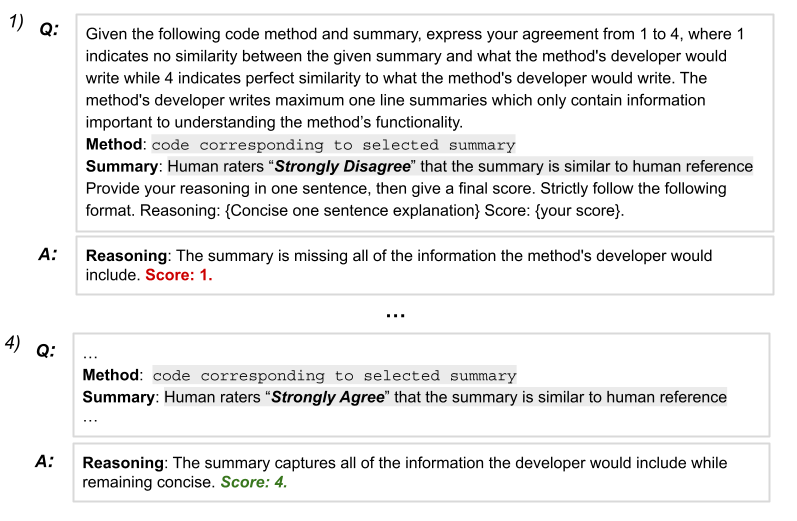
Figure 8: 4-shot Verbalized Confidence Examples

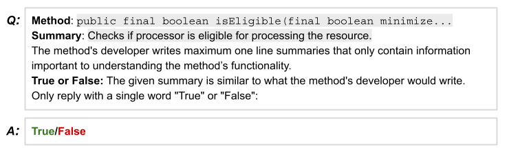
Figure 9: Reflective Logit Prompt

VI Discussion: Threats & Limitations

VI-A Metrics Limitations

The notion of correctness in our work is based on similarity to human-produced summaries. However, human developers have different intents (how/what/why) when writing summaries [1, 45]. These different intents are not captured by the similarity metrics. A reliable way of integrating intent into summary evaluation metrics remains for future work.

That said, it is important to note that prior work indicates that human-produced summaries are inherently valuable [22] and that the measure we used is an excellent proxy of human perceptions of similarity to human summaries [9, 21].

VI-B Experimental Design

In this paper, we primarily experimented with two programming languages, two prompting techniques, three models, and primarily with one similarity metric. Our findings in this paper are limited to these components. Prompting techniques can vary greatly, and the findings may differ significantly based on the prompting technique, as well as the programming language and metric used. Addressing all the languages, models, and prompting techniques is beyond the scope of this paper. However, Java and Python are two very different programming languages, and the models we used exhibit diversity in size and training. We believe that our findings will be well-generalized beyond these languages, models, and other parameters.

VI-C Why not temperature scaling?

Platt scaling is a popular and widely used rescaling strategy. However, another very popular rescaling technique is temperature scaling, which is found to be better than Platt scaling in certain scenarios. In this paper, we could not use temperature scaling because it requires access to complete softmax layers, which are unavailable from the OpenAI and TogetherAI APIs. In the future, we hope to incorporate temperature scaling into our experiments when we have access to the complete softmax layer.

VII Related Work

LLMs are widely used in many software engineering tasks [46, 47], including code summarization [18, 4]. Though LLMs are drawing attention from the community, it is well-known that they generate more buggy text/code than fixed text/code [6]. Consequently, the reliability of the model-generated output remains very low. To address this reliability issue, researchers have started looking into calibration in Software Engineering [40, 48]. Calibration is a well-studied domain in NLP [39], primarily for classification problems where model log-probabilities are used as a measure of model confidence.

Some interesting progress has been made in self-evaluation as well, where the model responds to its own generated solutions [49]. Though calibration is also being studied in the SE community [40, 48], to the best of our knowledge, there is no study on calibration for generative models for code summarization. Code summarization metrics also pose a unique challenge. Unlike program repair or program synthesis, the metrics used for code summarization are continuous values. In this paper, we explore thresholding these similarity metrics.

In SE, LLMs are increasingly popular, but questions about reliability persist. We anticipate more studies on calibration for different problems in the near future to enhance the reliability of model output.

VIII Conclusion

Code summaries are valuable to maintainers, and LLMs can generate good summaries from code. However, LLM-generated summary quality is very variable: sometimes similar to human-written summaries, and sometimes not. This indicates a need for developers to know when a summary might be sufficiently similar to a human-written summary. This is a calibration problem: can the model provide a reliable indication of its confidence that a generated summary is “good enough”? We address this problem by selecting a metric known from the literature to be a good proxy for similarity to human-produced summaries, and then threshold this metric to get an indication of sufficient similarity. We then show how the use of in-context learning, together with Platt scaling, provides a well-calibrated measure of confidence in generated summaries. Finally, our code and dataset are made available anonymously at https://doi.org/10.5281/zenodo.10858304.

References

- [1] X. Hu, X. Xia, D. Lo, Z. Wan, Q. Chen, and T. Zimmermann, “Practitioners’ expectations on automated code comment generation,” in Proceedings of the 44th International Conference on Software Engineering, 2022, pp. 1693–1705.
- [2] C. Zhang, J. Wang, Q. Zhou, T. Xu, K. Tang, H. Gui, and F. Liu, “A survey of automatic source code summarization,” Symmetry, vol. 14, no. 3, p. 471, 2022.
- [3] Y. Zhu and M. Pan, “Automatic code summarization: A systematic literature review,” arXiv preprint arXiv:1909.04352, 2019.
- [4] T. Ahmed, K. Pai, P. Devanbu, and E. T. Barr, “Automatic semantic augmentation of language model prompts (for code summarization),” in 2024 IEEE/ACM 46th International Conference on Software Engineering (ICSE). Los Alamitos, CA, USA: IEEE Computer Society, apr 2024, pp. 1004–1004. [Online]. Available: https://doi.ieeecomputersociety.org/
- [5] N. Nashid, M. Sintaha, and A. Mesbah, “Retrieval-based prompt selection for code-related few-shot learning,” in 2023 IEEE/ACM 45th International Conference on Software Engineering (ICSE). IEEE, 2023, pp. 2450–2462.
- [6] K. Jesse, T. Ahmed, P. T. Devanbu, and E. Morgan, “Large language models and simple, stupid bugs,” in 2023 IEEE/ACM 20th International Conference on Mining Software Repositories (MSR). IEEE, 2023, pp. 563–575.
- [7] R. Pan, A. R. Ibrahimzada, R. Krishna, D. Sankar, L. P. Wassi, M. Merler, B. Sobolev, R. Pavuluri, S. Sinha, and R. Jabbarvand, “Lost in translation: A study of bugs introduced by large language models while translating code,” in 2024 IEEE/ACM 46th International Conference on Software Engineering (ICSE). IEEE Computer Society, 2024, pp. 866–866.
- [8] F. Tambon, A. M. Dakhel, A. Nikanjam, F. Khomh, M. C. Desmarais, and G. Antoniol, “Bugs in large language models generated code,” arXiv preprint arXiv:2403.08937, 2024.
- [9] S. Haque, Z. Eberhart, A. Bansal, and C. McMillan, “Semantic similarity metrics for evaluating source code summarization,” in Proceedings of the 30th IEEE/ACM International Conference on Program Comprehension, 2022, pp. 36–47.
- [10] G. Sridhara, E. Hill, D. Muppaneni, L. Pollock, and K. Vijay-Shanker, “Towards automatically generating summary comments for java methods,” in Proceedings of the 25th IEEE/ACM international conference on Automated software engineering, 2010, pp. 43–52.
- [11] X. Xia, L. Bao, D. Lo, Z. Xing, A. E. Hassan, and S. Li, “Measuring program comprehension: A large-scale field study with professionals,” IEEE Transactions on Software Engineering, vol. 44, no. 10, pp. 951–976, 2017.
- [12] Z. Feng, D. Guo, D. Tang, N. Duan, X. Feng, M. Gong, L. Shou, B. Qin, T. Liu, D. Jiang et al., “Codebert: A pre-trained model for programming and natural languages,” in Findings of the Association for Computational Linguistics: EMNLP 2020, 2020, pp. 1536–1547.
- [13] W. U. Ahmad, S. Chakraborty, B. Ray, and K.-W. Chang, “Unified pre-training for program understanding and generation,” arXiv preprint arXiv:2103.06333, 2021.
- [14] T. Ahmed and P. Devanbu, “Multilingual training for software engineering,” in Proceedings of the 44th International Conference on Software Engineering, 2022, pp. 1443–1455.
- [15] Y. Wang, W. Wang, S. Joty, and S. C. Hoi, “Codet5: Identifier-aware unified pre-trained encoder-decoder models for code understanding and generation,” arXiv preprint arXiv:2109.00859, 2021.
- [16] R. Bommasani, D. A. Hudson, E. Adeli, R. Altman, S. Arora, S. von Arx, M. S. Bernstein, J. Bohg, A. Bosselut, E. Brunskill et al., “On the opportunities and risks of foundation models,” arXiv preprint arXiv:2108.07258, 2021.
- [17] T. Brown, B. Mann, N. Ryder, M. Subbiah, J. D. Kaplan, P. Dhariwal, A. Neelakantan, P. Shyam, G. Sastry, A. Askell et al., “Language models are few-shot learners,” Advances in neural information processing systems, vol. 33, pp. 1877–1901, 2020.
- [18] T. Ahmed and P. Devanbu, “Few-shot training llms for project-specific code-summarization,” in Proceedings of the 37th IEEE/ACM International Conference on Automated Software Engineering, 2022, pp. 1–5.
- [19] D. Roy, S. Fakhoury, and V. Arnaoudova, “Reassessing automatic evaluation metrics for code summarization tasks,” in Proceedings of the 29th ACM Joint Meeting on European Software Engineering Conference and Symposium on the Foundations of Software Engineering, 2021, pp. 1105–1116.
- [20] E. Shi, Y. Wang, L. Du, J. Chen, S. Han, H. Zhang, D. Zhang, and H. Sun, “On the evaluation of neural code summarization,” in Proceedings of the 44th international conference on software engineering, 2022, pp. 1597–1608.
- [21] A. Mastropaolo, M. Ciniselli, M. Di Penta, and G. Bavota, “Evaluating code summarization techniques: A new metric and an empirical characterization,” 2024.
- [22] S. Stapleton, Y. Gambhir, A. LeClair, Z. Eberhart, W. Weimer, K. Leach, and Y. Huang, “A human study of comprehension and code summarization,” in Proceedings of the 28th International Conference on Program Comprehension, 2020, pp. 2–13.
- [23] K. Papineni, S. Roukos, T. Ward, and W.-J. Zhu, “Bleu: a method for automatic evaluation of machine translation,” in Proceedings of the 40th annual meeting of the Association for Computational Linguistics, 2002, pp. 311–318.
- [24] C.-Y. Lin, “Rouge: A package for automatic evaluation of summaries,” in Text summarization branches out, 2004, pp. 74–81.
- [25] S. Banerjee and A. Lavie, “Meteor: An automatic metric for mt evaluation with improved correlation with human judgments,” in Proceedings of the acl workshop on intrinsic and extrinsic evaluation measures for machine translation and/or summarization, 2005, pp. 65–72.
- [26] D. S. Wilks, “On the combination of forecast probabilities for consecutive precipitation periods,” in Weather and Forecasting, vol. 5, 1990, pp. 640––650.
- [27] J. Platt et al., “Probabilistic outputs for support vector machines and comparisons to regularized likelihood methods,” Advances in large margin classifiers, vol. 10, no. 3, pp. 61–74, 1999.
- [28] B. Zadrozny and C. Elkan, “Obtaining calibrated probability estimates from decision trees and naive bayesian classifiers,” in Icml, vol. 1, 2001, pp. 609–616.
- [29] ——, “Transforming classifier scores into accurate multiclass probability estimates,” in Proceedings of the eighth ACM SIGKDD international conference on Knowledge discovery and data mining, 2002, pp. 694–699.
- [30] S. Lu, D. Guo, S. Ren, J. Huang, A. Svyatkovskiy, A. Blanco, C. Clement, D. Drain, D. Jiang, D. Tang et al., “Codexglue: A machine learning benchmark dataset for code understanding and generation,” arXiv preprint arXiv:2102.04664, 2021.
- [31] S. Robertson, H. Zaragoza et al., “The probabilistic relevance framework: Bm25 and beyond,” Foundations and Trends® in Information Retrieval, vol. 3, no. 4, pp. 333–389, 2009.
- [32] D. Guo, Q. Zhu, D. Yang, Z. Xie, K. Dong, W. Zhang, G. Chen, X. Bi, Y. Wu, Y. Li et al., “Deepseek-coder: When the large language model meets programming–the rise of code intelligence,” arXiv preprint arXiv:2401.14196, 2024.
- [33] B. Roziere, J. Gehring, F. Gloeckle, S. Sootla, I. Gat, X. E. Tan, Y. Adi, J. Liu, T. Remez, J. Rapin et al., “Code llama: Open foundation models for code,” arXiv preprint arXiv:2308.12950, 2023.
- [34] H. Touvron, L. Martin, K. Stone, P. Albert, A. Almahairi, Y. Babaei, N. Bashlykov, S. Batra, P. Bhargava, S. Bhosale et al., “Llama 2: Open foundation and fine-tuned chat models,” arXiv preprint arXiv:2307.09288, 2023.
- [35] J. Wei, X. Wang, D. Schuurmans, M. Bosma, F. Xia, E. Chi, Q. V. Le, D. Zhou et al., “Chain-of-thought prompting elicits reasoning in large language models,” Advances in neural information processing systems, vol. 35, pp. 24 824–24 837, 2022.
- [36] A. Conneau, D. Kiela, H. Schwenk, L. Barrault, and A. Bordes, “Supervised learning of universal sentence representations from natural language inference data,” arXiv preprint arXiv:1705.02364, 2017.
- [37] N. Reimers and I. Gurevych, “Sentence-bert: Sentence embeddings using siamese bert-networks,” arXiv preprint arXiv:1908.10084, 2019.
- [38] T. Zhang, V. Kishore, F. Wu, K. Q. Weinberger, and Y. Artzi, “Bertscore: Evaluating text generation with bert,” arXiv preprint arXiv:1904.09675, 2019.
- [39] C. Guo, G. Pleiss, Y. Sun, and K. Q. Weinberger, “On calibration of modern neural networks,” in International conference on machine learning. PMLR, 2017, pp. 1321–1330.
- [40] Z. Zhou, C. Sha, and X. Peng, “On calibration of pre-trained code models,” in 2024 IEEE/ACM 46th International Conference on Software Engineering (ICSE). IEEE Computer Society, 2024, pp. 861–861.
- [41] G. W. Brier, “Verification of forecasts expressed in terms of probability,” Monthly weather review, vol. 78, no. 1, pp. 1–3, 1950.
- [42] M. P. Naeini, G. Cooper, and M. Hauskrecht, “Obtaining well calibrated probabilities using bayesian binning,” in Proceedings of the AAAI conference on artificial intelligence, vol. 29, no. 1, 2015.
- [43] Wetter und Klima - Deutscher Wetterdienst - Our services - Skill measure: Brier Skill Score. [Online]. Available: https://www.dwd.de/EN/ourservices/seasonals_forecasts/forecast_reliability.html
- [44] J. B. Wezerek, Gus. How Good Are FiveThirtyEight Forecasts? FiveThirtyEight. [Online]. Available: https://projects.fivethirtyeight.com/checking-our-work/
- [45] M. Geng, S. Wang, D. Dong, H. Wang, G. Li, Z. Jin, X. Mao, and X. Liao, “Large language models are few-shot summarizers: Multi-intent comment generation via in-context learning,” in Proceedings of the 46th IEEE/ACM International Conference on Software Engineering, 2024, pp. 1–13.
- [46] A. Fan, B. Gokkaya, M. Harman, M. Lyubarskiy, S. Sengupta, S. Yoo, and J. M. Zhang, “Large language models for software engineering: Survey and open problems,” arXiv preprint arXiv:2310.03533, 2023.
- [47] X. Hou, Y. Zhao, Y. Liu, Z. Yang, K. Wang, L. Li, X. Luo, D. Lo, J. Grundy, and H. Wang, “Large language models for software engineering: A systematic literature review,” arXiv preprint arXiv:2308.10620, 2023.
- [48] D. Zhang, X. Zhang, C. Bansal, P. Las-Casas, R. Fonseca, and S. Rajmohan, “Pace: Prompting and augmentation for calibrated confidence estimation with gpt-4 in cloud incident root cause analysis,” arXiv preprint arXiv:2309.05833, 2023.
- [49] S. Kadavath, T. Conerly, A. Askell, T. Henighan, D. Drain, E. Perez, N. Schiefer, Z. Hatfield-Dodds, N. DasSarma, E. Tran-Johnson et al., “Language models (mostly) know what they know,” arXiv preprint arXiv:2207.05221, 2022.