A characterization of entangled two-qubit states via partial-transpose-moments

Abstract

Although quantum entanglement is an important resource, its characterization is quite challenging. The partial transposition is a common method to detect bipartite entanglement. In this paper, the authors study the partial-transpose(PT)-moments of two-qubit states, and completely describe the whole region, composed of the second and third PT-moments, for all two-qubit states. Furthermore, they determine the accurate region corresponding to all entangled two-qubit states. The states corresponding to those boundary points of the whole region, and to the border lines between separable and entangled states are analyzed. As an application, they characterize the entangled region of PT-moments for the two families of Werner states and Bell-diagonal states. The relations between entanglement and the pairs of PT-moments are revealed from these typical examples. They also numerically plot the whole region of possible PT-moments for all two-qubit X-states, and find that this region is almost the same as the whole region of PT-moments for all two-qubit states. Moreover, they extend their results to detect the entanglement of multiqubit states. By utilizing the PT-moment-based method to characterize the entanglement of the multiqubit states mixed by the GHZ and W states, they propose an operational way of verifying the genuine entanglement in such states.

1 Introduction

Characterizing entanglement is a key task in quantum information science because the entanglement is a necessary resource in various information processing tasks [1, 2, 3, 4]. To detect entanglement, Peres firstly proposed a necessary condition for all separable states [5], i.e., the well-known positive-partial-transpose (PPT) criterion. It states that a bipartite state is entangled whenever it violates the PPT criterion, i.e., its partial transpose (PT) has at least one negative eigenvalue. Such entangled states are called non-positive-partial-transpose (NPT) states. Subsequently, Horodecki’s family specified that the PPT criterion is a necessary and sufficient condition [6] for the separable states supported on $\mathbb{C}^{m}\otimes\mathbb{C}^{n}$ when $mn\leqslant 6$. Due to the PPT criterion, the entanglement detection has been reduced to detect the entangled states retaining the PPT property, also known as the PPT entangled states. A fundamental tool to detect PPT entangled states is the so-called entanglement witness (EW) [7]. It has been shown that an EW can detect PPT entangled states if and only if it is non-decomposable [8]. Thus much effort has been devoted to constructing non-decomposable EWs [9, 10, 11]. In particular, the partial transpose of an NPT state can be viewed as an EW, though it can only detect NPT states.

The PPT criterion implies that the negative eigenvalues of the partial transpose of a bipartite state $\rho_{AB}$ are a signature of the entanglement in $\rho_{AB}$. Denote by $\rho_{AB}^{\Gamma_{A}}$ and $\rho_{AB}^{\Gamma_{B}}$ the partial transposes of $\rho_{AB}$ with respect to system $A$ and $B$ respectively. Note that the two partial transposes share the same spectrum. Hence, for simplicity, we use $\rho_{AB}^{\Gamma}$ to denote one of the two partial transposes. Depending on the spectrum of $\rho^{\Gamma}_{AB}$, a well-known computable entanglement measure called the logarithm of negativity was introduced in Ref. [12]. It has various operational interpretations, including the upper bound of the entanglement distillation rate [13], the bound on teleportation capacity and the entanglement cost under a large operation set [14, 15].

The PPT criterion is actually a mathematical tool commonly used in the theoretical scenario. For a given bipartite state $\rho_{AB}$ of system $AB$, it is straightforward to check whether the PPT criterion is violated. Nevertheless, in the practical scenario, the detection of entanglement is not so direct. On the one hand, the partial transposition of an operator is not a physical operation, and it cannot be implemented directly in experiments. On the other hand, in actual experiments, the quantum state is unknown, unless the resource-inefficient quantum state tomography is performed [16]. More generally, the realizations of effective entanglement criteria usually consume exponential resources, and efficient criteria often perform poorly without prior knowledge [17]. Therefore, it is necessary to develop experimentally efficient methods to detect entanglement based on the measurable observables. Recently, a realizable entanglement detection method based on the PPT criterion by investigating the so-called partial transpose moments (PT-moments) defined by

$$p_{k}:=\operatorname{Tr}\left(\left[\rho^{\Gamma}_{AB}\right]^{k}\right)$$ (1.1)

has been introduced in Ref. [16]. Although the PT-moments are nonlinear functions of the state $\rho_{AB}$ depending on the spectrum of $\rho^{\Gamma}_{AB}$, it has been shown, recently, in Refs. [18, 19] that the PT-moments can be efficiently measured from local randomized measurements. Specifically, the PT-moment can be measured as an expectation value of an $n$-copy cyclic permutation operator [18], and the protocol of measurements only requires single-qubit control in Noisy Intermediate Scale Quantum (NISQ) devices [18, Fig. 1b]. Furthermore, Ref. [20] shows that with the assistance of machine learning, one can extract the negativity just from the third PT-moment $p_{3}$. The latter can be estimated based on the random unitary evolution and local measurements on a single-copy quantum state [21]. Later, Liu et al. extended the notion of PT-moments to that of permutation moments [22], and proposed a framework for designing multipartite entanglement criteria based on permutation moments. Moreover, the PT-moments provide an entanglement detection method via the moments of the state $\rho_{AB}$ itself. Not only this, there are several proposals of testing and characterizing entanglement via second-order and special higher-order moments of various observables (like the position, momentum, annihilation and creation operators of qubits and qudits [23, 24, 25, 26]) has been presented, and their matrices have been developed by Werner Vogel et al. for both bipartite [27, 28] and multipartite (or multimode) [29, 30] systems.

The measurability of PT-moments bridges the practical limitations of the PPT criterion, and allows it to be used for experimental entanglement detection. In spite of this, the PT-moments cannot provide a more powerful criterion than the PPT criterion for entanglement detection. On the other word, we cannot detect the PPT entangled states based on the knowledge of PT-moments. Moreover, we cannot use PT-moments to distinguish the set of PT-moments of all separable states $\sigma_{AB}$ from that of all states $\rho_{AB}$ on the same underlying space because both of the two sets are the same. Hence, in order to dectect entanglement utilizing the PT-moments, it is necessary to characterize the PT-moments of all NPT entangled states. Basically, we consider the characterization of the set of PT-moments of all entangled states supported on $\mathbb{C}^{m}\otimes\mathbb{C}^{n}$, where $m,n\geqslant 2$. In such a framework, the computational complexity increases exponentially as $m$ and $n$ increase. Due to the fundamental importance of the toy model of the two-qubit system, we focus on the derivation in the two-qubit system. Since there is no PPT entangled state of the two-qubit system, the PT-moment-based method has the ability to characterize the set of all two-qubit entangled states. Proposition 2.1 is constructed and can be viewed as the identification of the set of PT-moments of all two-qubit separable states. In this short report, we will identify the set of PT-moments of all entangled two-qubit states in Theorem 3.1. By doing so, in fact, we give an equivalent, but experimentally measurable criterion of entangled two-qubit states. Such a criterion is also illustrated in Fig. 1 by identifying the dividing line between the set of separable states and that of entangled states. Then we apply this experimentally measurable criterion to detect the entanglement of several widely used states. We also demonstrate the relations between entanglement and the pairs of PT moments for these typical examples in Figs. 2 - 5. Analogously to these figures, several proposals of characterizing the entanglement of two-qubit states by plotting one entanglement measure or witness versus others have been reported in a number of interesting papers [31, 32, 33, 34].

From Eq. (1.1) one can equivalently calculate each $p_{k}$ as the sum of all $x_{i}^{k}$, where $x_{i}$’s are the eigenvalues of $\rho_{AB}^{\Gamma}$. Thus, the calculation of $p_{k}$ is closely related to the spectrum of $\rho^{\Gamma}_{AB}$. Due to this close relation, it is necessary to deeply understand some properties of the spectrum of $\rho^{\Gamma}_{AB}$. Recently, several results on the spectrum of $\rho^{\Gamma}_{AB}$ have been developed [35, 36, 37, 38]. Specifically, it follows from Ref. [35] that the partial transpose $\rho^{\Gamma}_{AB}$ supported on $\mathbb{C}^{m}\otimes\mathbb{C}^{n}$ has no more than $(m-1)(n-1)$ negative eigenvalues, and all eigenvalues of $\rho^{\Gamma}_{AB}$ fall within the closed interval $\left[-\tfrac{1}{2},1\right]$. Therefore, when considering the PT-Moment problem for bipartite space $\mathbb{C}^{2}\otimes\mathbb{C}^{3}$, we will encounter more difficulties of calculating the PT-moments because the number of negative eigenvalues of $\rho^{\Gamma}_{AB}$ could be one or two. In view of this, the identification of all PT-moments of the states supported on $\mathbb{C}^{m}\otimes\mathbb{C}^{n}$ with $mn\geqslant 6$ could be much more complicated than the case of two-qubit states.

The paper is organized as follows. In Sec. 3, we present our main result with its proof being delayed to Appendix A. In Sec. 4, some examples of two-qubit and multiqubit states are given in terms of our main result. Finally, we conclude in Sec. 5.

2 Preliminaries

To see how the PT-moments can be used in entanglement detection, suppose that $\rho_{AB}$ is a bipartite state supported on the Hilbert space $\mathcal{H}_{A}\otimes\mathcal{H}_{B}\cong\mathbb{C}^{d_{A}}\otimes\mathbb{C}^{d_{B}}$, and we know the PT-moment $p_{k}$ of $\rho_{AB}$ for any $k\in[1,d]$, where $d=d_{A}d_{B}$ is the global dimension. Denote by $(x_{1},\ldots,x_{d})$ the spectrum of $\rho^{\Gamma}_{AB}$, where the eigenvalues $x_{1},\ldots,x_{d}$ are always assumed to be sorted in descending order, unless otherwise stated. Obviously, the PT-moment for each $k$ is formulated as

$$p_{k}=\sum_{i=1}^{d}x_{i}^{k}.$$ (2.1)

Then Ref. [39] shows that the spectrum of $\rho^{\Gamma}_{AB}$ can be determined with all known PT-moments, for which whether $\rho_{AB}$ is an NPT state can be verified. This process provides the PT-moment-based entanglement detection. Hereafter, we call $\boldsymbol{p}^{(d)}=(p_{1},\ldots,p_{d})$ the PT-moment vector, and always assume that $p_{1}=1$ for convenience.

In Ref. [16], the authors studied a specific problem as follows.

PT-Moment problem: Given the PT-moments of order $n$, is there a separable state compatible with the data? More technically formulated, given the real vector

$$\boldsymbol{p}^{(n)}=(p_{1},\ldots,p_{n}),$$ (2.2)

is there a separable quantum state $\rho_{AB}$ such that for each $1\leq k\leq n$,

$$p_{k}=\operatorname{Tr}\left(\left[\rho^{\Gamma}_{AB}\right]^{k}\right)?$$ (2.3)

It is natural to consider the detection of entanglement in $\rho_{AB}$ from a few of the PT-moments due to the difficulty in measuring all the PT-moments. In fact, the authors derived a necessary and sufficient condition for the PT-Moment problem when the order $n$ is three in Ref. [16]. It states that there is a separable state supported on $\mathbb{C}^{d}$ compatible with the given vector $(q_{1},q_{2},q_{3})$ if and only if

$$\begin{aligned} &\frac{1}{d}\leqslant q_{2}\leqslant 1,\\ &\Phi^{+}_{d}(q_{2})\geqslant q_{3}\geqslant\phi_{d}(q_{2}),\end{aligned}$$ (2.4)

where

$$\begin{aligned} \Phi^{+}_{d}(q_{2})&:=(d-1)y^{3}+[1-(d-1)y]^{3},\\ \phi_{d}(q_{2})&:=\tau(q_{2})x^{3}+(1-\tau(q_{2})x)^{3},\end{aligned}$$ (2.5)

for $\tau(q_{2}):=\lfloor\frac{1}{q_{2}}\rfloor$, and via

$$\begin{aligned} y&\equiv y(q_{2}):=\frac{d-1-\sqrt{(d-1)(dq_{2}-1)}}{d(d-1)},\\ x&\equiv x(q_{2}):=\frac{\tau(q_{2})+\sqrt{\tau(q_{2})[(\tau(q_{2})+1)q_{2}-1]}}{\tau(q_{2})(\tau(q_{2})+1)}.\end{aligned}$$ (2.6)

Based on this result and in view of the result from Ref. [40], we get a more precise answer to the PT-Moment problem for two-qubit states.

Proposition 2.1.

There is a separable two-qubit state $\rho_{AB}$ compatible with the given PT-moment vector $\boldsymbol{p}^{(4)}=(p_{1},p_{2},p_{3},p_{4})$, where every PT moment $p_{k}$ is defined by Eq. (1.1), if and only if the following two inequalities hold:

$$\frac{1}{4}\leqslant p_{2}\leqslant 1,$$ (2.7)

$$\Phi^{+}_{4}(p_{2})\geqslant p_{3}\geqslant\phi_{4}(p_{2}),$$ (2.8)

where $\Phi^{+}_{4}(p_{2})=\frac{3(6p_{2}-1)+\sqrt{3}(4p_{2}-1)^{\frac{3}{2}}}{24}$, and $\phi_{4}(p_{2})$ can be rewritten as a piecewise function:

$$\phi_{4}(p_{2})=\begin{cases}\frac{3p_{2}-1}{2},&\text{if }p_{2}\in[\frac{1}{2},1],\\ \frac{2(9p_{2}-2)-\sqrt{2}(3p_{2}-1)^{\frac{3}{2}}}{18},&\text{if }p_{2}\in[\frac{1}{3},\frac{1}{2}],\\ \frac{3(6p_{2}-1)-\sqrt{3}(4p_{2}-1)^{\frac{3}{2}}}{24},&\text{if }p_{2}\in[\frac{1}{4},\frac{1}{3}].\end{cases}$$ (2.9)

This is a continuous function for $p_{2}\in[\frac{1}{4},1]$.

3 Main result

In this section we propose a PT-moment-based separability criterion for two-qubit states. It relies on the accurate characterization of the set of the PT-moment vectors corresponding to entangled two-qubit states as follows.

Theorem 3.1.

There is an entangled two-qubit state $\rho_{AB}$ compatible with the given PT-moment vector $\boldsymbol{p}^{(4)}=(p_{1},p_{2},p_{3},p_{4})$, where every PT moment $p_{k}$ is defined by Eq. (1.1), if and only if both the following two inequalities hold:

$$\frac{1}{3}<p_{2}\leqslant 1,$$ (3.1)

$$\phi_{4}(p_{2})>p_{3}\geqslant\Phi^{-}_{4}(p_{2}),$$ (3.2)

where $\phi_{4}(p_{2})$ is given by Eq. (2.9), and

$$\Phi^{-}_{4}(p_{2}):=\frac{3(6p_{2}-1)-\sqrt{3}(4p_{2}-1)^{\frac{3}{2}}}{24}.$$ (3.3)

Note here that $\phi_{4}(p_{2})\equiv\Phi^{-}_{4}(p_{2})$ for all $p_{2}\in[\frac{1}{4},\frac{1}{3}]$. This amounts to say that the two-qubit state $\rho_{AB}$ with purity $p_{2}\in[\frac{1}{4},\frac{1}{3}]$ must be separable.

Proof.

The details are put in Appendix A. ∎

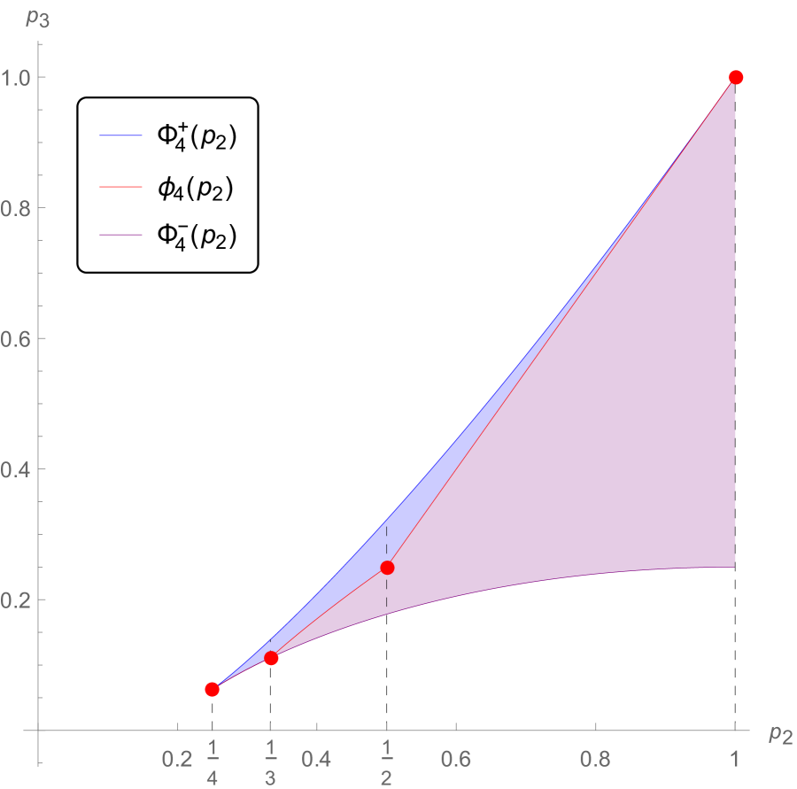
Figure 1: (Color Online) The PT-moment pair $(p_{2},p_{3})$ of two-qubit state $\rho_{AB}$ falls within the light blue colored region with upper and lower boundaries iff two-qubit $\rho_{AB}$ is separable; the pair $(p_{2},p_{3})$ of PT-moments of two-qubit state $\rho_{AB}$ falls within the purple colored region with only the lower boundary iff two-qubit $\rho_{AB}$ is entangled. The coordinates of these red points (from left to right) correspond to $(\frac{1}{4},\frac{1}{16})$( only the completely mixed state), $(\frac{1}{3},\frac{1}{9}),(\frac{1}{2},\frac{1}{4}),(1,1)$(the set of separable pure states), respectively; the coordinate of only the purple point is $(1,\frac{1}{4})$, corresponding to the family of all maximally entangled states.

Based on the characterization of the set of PT-moment vectors of entangled two-qubit states, we further obtain that of all two-qubit states.

Corollary 3.2.

For any two-qubit state $\rho_{AB}$, its PT-moment vector $\boldsymbol{p}^{(4)}=(p_{1},p_{2},p_{3},p_{4})$ satisfies that

$$\Phi^{+}_{4}(p_{2})\geqslant p_{3}\geqslant\Phi^{-}_{4}(p_{2}),$$ (3.4)

where $\Phi^{\pm}_{4}(p_{2})=\frac{3(6p_{2}-1)\pm\sqrt{3}(4p_{2}-1)^{\frac{3}{2}}}{24}$ for $p_{2}\in[\frac{1}{4},1]$.

Denote by $R_{\text{sep}}$ the set of pairs $(p_{2},p_{3})$ of PT-moments of all separable two-qubit states; and by $R_{\text{ent}}$ that of all entangled two-qubit states. That is,

$$\begin{aligned} R_{\text{sep}}&:=\left\{(p_{2},p_{3}):\tfrac{1}{4}\leqslant p_{2}\leqslant 1,\Phi^{+}_{4}(p_{2})\geqslant p_{3}\geqslant\phi_{4}(p_{2})\right\},\\ R_{\text{ent}}&:=\left\{(p_{2},p_{3}):\tfrac{1}{4}\leqslant p_{2}\leqslant 1,\phi_{4}(p_{2})>p_{3}\geqslant\Phi^{-}_{4}(p_{2})\right\}.\end{aligned}$$ (3.5)

Both of them are plotted in Fig 1. In addition, we present specific states corresponding to boundary curves of $R_{\mathrm{sep}/\mathrm{ent}}$ in Fig 1:

• The vertical line $p_{2}=1$: All pure states.

• The curve $p_{3}=\Phi^{+}_{4}(p_{2})$:

  $$\lambda(|00\rangle\langle 00|+|01\rangle\langle 01|+|10\rangle\langle 10|)+(1-3\lambda)|11\rangle\langle 11|$$ (3.6)

  for $\lambda\in[0,\frac{1}{4}]$.

• The curve $p_{3}=\Phi^{-}_{4}(p_{2})$: All Werner states.

Specific states corresponding to the inner border lines:

• The curve $p_{3}=\phi_{4}(p_{2})(p_{2}\in[\tfrac{1}{2},1])$:

  $$\lambda|00\rangle\langle 00|+(1-\lambda)|01\rangle\langle 01|$$ (3.7)

  for $\lambda\in[0,1]$.

• The curve $p_{3}=\phi_{4}(p_{2})$ with $p_{2}\in[\tfrac{1}{3},\tfrac{1}{2}]$:

  $$\lambda|00\rangle\langle 00|+\lambda|01\rangle\langle 01|+(1-2\lambda)|10\rangle\langle 10|$$ (3.8)

  for $\lambda\in[\tfrac{1}{3},\tfrac{1}{2}]$.

• The curve $p_{3}=\phi_{4}(p_{2})$ with $p_{2}\in[\tfrac{1}{4},\tfrac{1}{3}]$: All separable Werner states.

Furthermore, we also calculate the areas of two regions: $A(R_{\text{sep}})=\frac{43}{2160}$ and $A(R_{\text{ent}})=\frac{443}{2160}$. There is an interesting question may be related to such two areas. That is, we may establish the joint probability density function (PDF)

$$f(p_{2},p_{3}):=\int\mathrm{d}\mu(\rho)\delta\left(p_{2}-\operatorname{Tr}\left(\left[\rho^{\Gamma}\right]^{2}\right)\right)\delta\left(p_{3}-\operatorname{Tr}\left(\left[\rho^{\Gamma}\right]^{3}\right)\right)$$ (3.9)

over the set of pairs $(p_{2},p_{3})$ for all two-qubit states, where $\mathrm{d}\mu(\rho)$ is the measure induced by Hilbert-Schmidt norm. Once we get the analytical expression of function $f$, then we may solve the following open question. That is,

$$\int_{R_{\mathrm{sep}}}f(p_{2},p_{3})\mathrm{d}p_{2}\mathrm{d}p_{3}\Big{/}\int_{R_{\mathrm{ent}}}f(p_{2},p_{3})\mathrm{d}p_{2}\mathrm{d}p_{3}$$ (3.10)

should be related to the ratio $\frac{\mathrm{vol}_{\mathrm{sep}}(\mathrm{D}\left(\mathbb{C}^{2}\otimes\mathbb{C}^{2}\right))}{\mathrm{vol}_{\mathrm{ent}}(\mathrm{D}\left(\mathbb{C}^{2}\otimes\mathbb{C}^{2}\right))}$, which is conjectured to be $\tfrac{8}{25}$ [41]. Hopefully, it sheds new light on this open question.

4 Application

In this section, as essential applications of our main result in Sec. 3, we construct examples, and use the PT-moment-based separability criterion in Theorem 3.1 to analyze the separability of these examples. We construct examples of the two-qubit system in Sec. 4.1, such as the Werner states, Bell-diagonal states, $X$-states. Then we also consider the multipartite entanglement, and construct examples of the multipartite system in Sec. 4.2, such as the convex sum of multiqubit GHZ and W states.

4.1 two-qubit systems

Example 4.1 (The family of Werner states).

In 1989, Werner analytically constructed a family of $\boldsymbol{U}\otimes\boldsymbol{U}$ invariant states to investigate local hidden variable (LHV) models [42]. As a toy model, we consider the two-qubit Werner states formulated as

$$\rho_{W}(w)=w|\psi^{-}\rangle\langle\psi^{-}|+(1-w)\frac{\mathbf{1}_{4}}{4}$$ (4.1)

where $|\psi^{-}\rangle=\frac{|01\rangle-|10\rangle}{\sqrt{2}}$ and $w\in[0,1]$. By calculation, the second and third PT-moments of two-qubit Werner state $\rho_{W}(w)$ are, respectively,

$$p_{2}=\frac{1+3w^{2}}{4}\quad\text{and}\quad p_{3}=\frac{-6w^{3}+9w^{2}+1}{16}.$$ (4.2)

Substituting $p_{2}$ and $p_{3}$ above into the two inequalities (3.1) and (3.2) in Theorem 3.1, one can verify both the two inequalities hold if and only if $w\in(\tfrac{1}{3},1]$. This is also equivalent to the well-known fact on the separability of Werner states [43] that $\rho_{W}(w)$ is entangled if and only if $w\in(\frac{1}{3},1]$. Eliminating the parameter $w\in[0,1]$, we find that the pair $(p_{2},p_{3})$ satisfies $p_{3}=\Phi^{-}_{4}(p_{2})$. It means the points fixed by the pairs $(p_{2},p_{3})$ corresponding to the set of entangled two-qubit Werner states are just lying on the lowest curve, i.e., the purple one in Fig 1.

Example 4.2 (The family of Bell-diagonal states).

The Bell-diagonal states [40] in the two-qubit system can be written as

$$\rho_{\text{Bell}}=\frac{1}{4}(\mathbb{1}_{4}+\sum_{i=1}^{3}t_{i}\sigma_{i}\otimes\sigma_{i}),$$ (4.3)

where $\sigma_{i}$ for $i=1,2,3$ are three Pauli operators as $\sigma_{1}=|0\rangle\langle 1|+|1\rangle\langle 0|$, $\sigma_{2}={\rm i}|0\rangle\langle 1|-{\rm i}|1\rangle\langle 0|$, $\sigma_{3}=|0\rangle\!\langle 0|-|1\rangle\!\langle 1|$. Hence, a Bell-diagonal state is specified by three real variables $t_{1},t_{2}$, and $t_{3}$ such that

$$\begin{cases}1-t_{1}-t_{2}-t_{3}\geqslant 0,\\ 1-t_{1}+t_{2}+t_{3}\geqslant 0,\\ 1+t_{1}-t_{2}+t_{3}\geqslant 0,\\ 1+t_{1}+t_{2}-t_{3}\geqslant 0.\end{cases}$$ (4.4)

Denote by $D_{\text{Bell}}$ the set of tuples $(t_{1},t_{2},t_{3})$ satisfying the system of inequalities Eq. (4.4). Because all the four eigenvalues of $\rho_{\text{Bell}}$ are in $[0,1]$, it follows from Eq. (4.3) that $t_{i}\in[-1,1]$ for $i=1,2,3$. That is, $D_{\text{Bell}}\subset[-1,1]^{3}$. Furthermore, the Bell-diagonal states can be geometrically described by a tetrahedron. One can show that a Bell-diagonal state is separable if and only if $\left\lvert\mspace{1.0mu}t_{1}\mspace{1.0mu}\right\rvert+\left\lvert\mspace{1.0mu}t_{2}\mspace{1.0mu}\right\rvert+\left\lvert\mspace{1.0mu}t_{3}\mspace{1.0mu}\right\rvert\leqslant 1$ holds. Geometrically, the set of Bell-diagonal states is a tetrahedron and the set of separable Bell-diagonal states is an octahedron [40] denoted by $D_{\text{Bellsep}}$. By calculation, all eigenvalues of $\rho^{\Gamma}_{\text{Bell}}$ are

$$\begin{aligned} x_{1}&=\frac{1+t_{1}-t_{2}-t_{3}}{4},~{}~{}x_{2}=\frac{1-t_{1}+t_{2}-t_{3}}{4},\\ x_{3}&=\frac{1+t_{1}+t_{2}+t_{3}}{4},~{}~{}x_{4}=\frac{1-t_{1}-t_{2}+t_{3}}{4}.\end{aligned}$$ (4.5)

It follows from Eq. (2.1) that

$$\begin{aligned} p_{2}&=\frac{1+\sum^{3}_{i=1}t^{2}_{i}}{4},\\ p_{3}&=\frac{1+6t_{1}t_{2}t_{3}+3\sum^{3}_{i=1}t^{2}_{i}}{16}.\end{aligned}$$ (4.6)

Next, we set $p_{2}\in[\frac{1}{4},1]$, and use $p_{2}$ to bound $p_{3}$ from above to below. It suffices to do the optimization:

$$\max_{(t_{1},t_{2},t_{3})\in D_{\text{Bell}}}~{}~{}g(t_{1},t_{2},t_{3})=t_{1}t_{2}t_{3}.$$ (4.7)

For the family of Bell diagonal states, we conclude

$$\Phi^{-}_{4}(p_{2})\leqslant p_{3}\leqslant\Phi^{\textsf{B}}_{4}(p_{2}),$$ (4.8)

where $\Phi^{\textsf{B}}_{4}(p_{2})$ is piecewisely functioned as

$$\Phi^{\textsf{B}}_{4}(p_{2}):=\begin{cases}\Phi^{+}_{4}(p_{2}),&\text{if }p_{2}\in[\frac{1}{4},\frac{1}{3}],\\ \frac{(18p_{2}-1)+2\sqrt{2}(3p_{2}-1)^{\frac{3}{2}}}{36},&\text{if }p_{2}\in[\frac{1}{3},\frac{1}{2}],\\ \frac{1}{4},&\text{if }p_{2}\in[\frac{1}{2},1].\\ \end{cases}$$ (4.9)

This conclusion follows from the result of the optimization problem in Eq. (4.7). We put the optimizing process and the proof of the inequality (4.8) in Appendix B. We add the curve of function $\Phi^{\textsf{B}}_{4}(p_{2})$ in Fig 2, and then the light green colored region with both upper and lower boundaries in Fig 2 is corresponding to the family of Bell-diagonal states from the inequality (4.8).

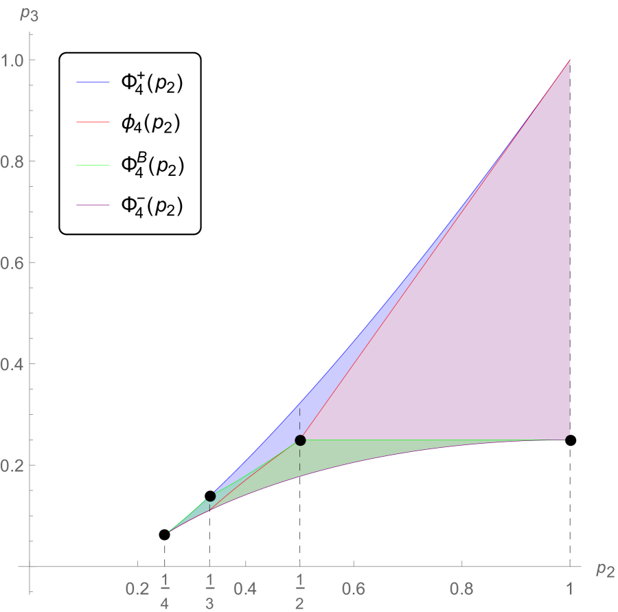
Figure 2: (Color online) The PT-moment pair $(p_{2},p_{3})$ for Bell-diagonal state $\rho_{\text{Bell}}$ falls within the light green colored region with both upper and lower boundaries; the coordinates of these black points are (from left to right): $\left(\frac{1}{4},\frac{1}{16}\right),\left(\frac{1}{3},\frac{5}{36}\right),\left(\frac{1}{2},\frac{1}{4}\right),\left(1,\frac{1}{4}\right)$.

Again, we formulate specific states corresponding to the border lines of the family of Bell-diagonal states below.

• The curve $p_{3}=\tfrac{1}{4}$ for $p_{2}\in[\tfrac{1}{2},1]$ corresponds to

  $$t|\phi^{+}\rangle\langle\phi^{+}|+(1-t)|\phi^{-}\rangle\langle\phi^{-}|$$ (4.10)

  for $t\in[0,1]$.

• The curve $p_{3}=\Phi^{\textsf{B}}_{4}(p_{2})$ for $p_{2}\in[\tfrac{1}{3},\tfrac{1}{2}]$ corresponds to

  $$\frac{1}{4}(\mathbb{1}_{4}+t\sigma_{1}\otimes\sigma_{1}+t\sigma_{2}\otimes\sigma_{2}+(1-2t)\sigma_{3}\otimes\sigma_{3})$$ (4.11)

  for $t\in[0,\frac{1}{3}]$.

• The curve $p_{3}=\Phi^{\textsf{B}}_{4}(p_{2})$ for $p_{2}\in[\tfrac{1}{4},\tfrac{1}{3}]$ corresponds to

  $$\frac{1}{4}(\mathbb{1}_{4}+t\sum_{i}\sigma_{i}\otimes\sigma_{i})$$ (4.12)

  for $t\in[0,\frac{1}{3}]$.

By calculation, we further obtain the fourth PT-moment

$$p_{4}=\frac{1+24t_{1}t_{2}t_{3}+6\sum^{3}\limits_{i=1}t^{2}_{i}+\sum^{3}\limits_{i=1}t^{4}_{i}+6\sum\limits_{1\leqslant i<j\leqslant 3}t^{2}_{i}t^{2}_{j}}{64}.$$ (4.13)

We can also plot the region of the tuple $(p_{2},p_{3},p_{4})$ for the family of Bell-diagonal states. Moreover, if we consider the negativity [14] in place of $p_{4}$, which is formulated by

$$\mathcal{N}(\rho_{\text{Bell}})=\tfrac{\left\lVert\mspace{1.0mu}\rho_{\text{Bell}}^{\Gamma}\mspace{1.0mu}\right\rVert_{1}-1}{2}$$ (4.14)

$$=\tfrac{1}{8}(\left\lvert\mspace{1.0mu}1+t_{1}-t_{2}-t_{3}\mspace{1.0mu}\right\rvert+\left\lvert\mspace{1.0mu}1-t_{1}+t_{2}-t_{3}\mspace{1.0mu}\right\rvert+\left\lvert\mspace{1.0mu}1+t_{1}+t_{2}+t_{3}\mspace{1.0mu}\right\rvert+\left\lvert\mspace{1.0mu}1-t_{1}-t_{2}+t_{3}\mspace{1.0mu}\right\rvert-4),$$

we can plot the region of the tuple $(p_{2},p_{3},\mathcal{N}(\rho_{\text{Bell}}))$, see Fig 3. The negativity of Bell-diagonal states increases as $p_{2}$ or $p_{3}$ increases. Since $p_{2}$ and $p_{3}$ can be efficiently measured in experiment, physically it means one can conveniently choose the Bell-diagonal states with larger entanglement by $p_{2}$ or $p_{3}$.

Bell-diagonal entangled states are assisted maximally entangled states [44], which can be decomposed as the convex combination of maximally entangled states. Therefore, with the help of the third party, Bell-diagonal entangled states can be transformed into maximally entangled pure states by local measurements and classical communication (LOCC). From the perspective of entanglement distillation, Bell-diagonal entangled states are resourceful and can widely be used in quantum information processing tasks.

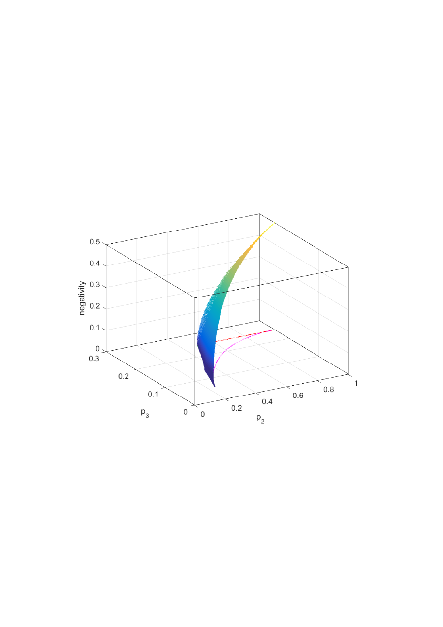
(a) The negativity of $\rho_{\rm Bell}$ versus the PT-moment pair $(p_{2},p_{3})$

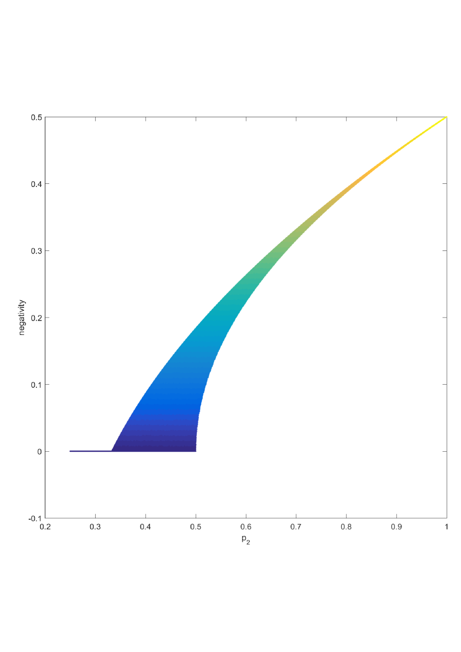
(b) The negativity of $\rho_{\rm Bell}$ versus the PT-moment $p_{2}$

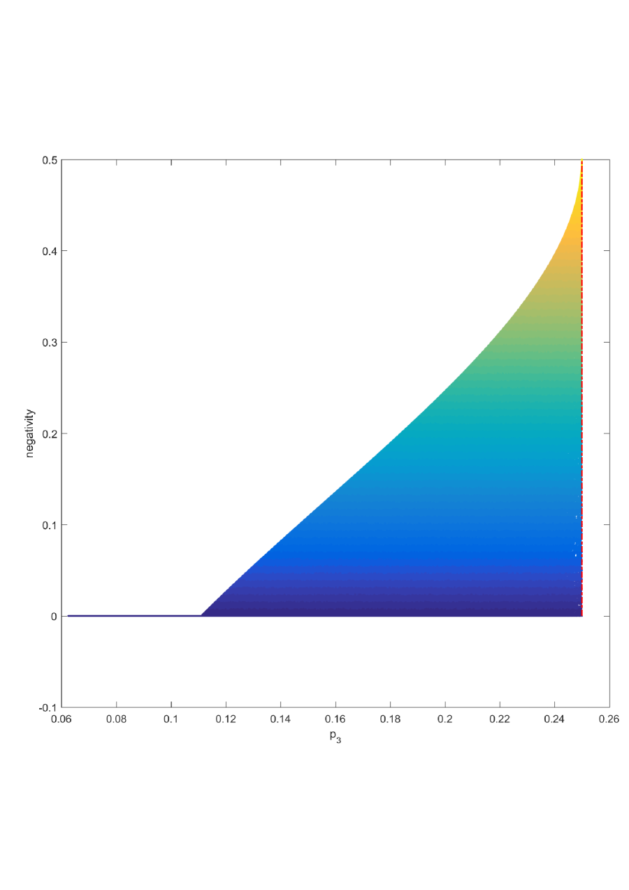
(c) The negativity of $\rho_{\rm Bell}$ versus the PT-moment $p_{3}$

Figure 3: (Color Online) Here, $\rho_{\rm Bell}$ represents a two-qubit Bell-diagonal state, and the pairs $(p_{2},p_{3})$ are sampled from the light green colored region in Fig. 2. The pairs $(p_{2},p_{3})$ on the left side of $\phi_{4}$-curve yield the negativity 0.

Example 4.3 (The family of two-qubit X-states).

The $X$-state is a name for the class of mixed states whose density matrix is in the X shape. Its quantum correlation such as quantum discord [45, 46, 47], one-way quantum deficit [48, 49], and quantum coherence including coherence concurrence [50] are investigated broadly. Attributing to the symmetry of $X$-state formally, the study of its quantumness seems to be more feasible than general mixed states. The pure states that can be transformed into an $X$-state with incoherent operations are also characterized in Ref. [51].

The so-called $X$-states in the two-qubit system are those states whose density matrices are of the form:

$$\rho_{\mathrm{X}}=\left(\begin{array}[]{cccc}\rho_{11}&0&0&\rho_{14}\\ 0&\rho_{22}&\rho_{23}&0\\ 0&\rho_{32}&\rho_{33}&0\\ \rho_{41}&0&0&\rho_{44}\end{array}\right).$$ (4.19)

The $X$-state $\rho_{\mathrm{X}}$ naturally satisfies the unit trace and the positivity conditions: (i) $\sum^{4}_{k=1}\rho_{kk}=1$ and (ii) $\rho_{22}\rho_{33}\geqslant\left\lvert\mspace{1.0mu}\rho_{23}\mspace{1.0mu}\right\rvert^{2}$ and $\rho_{11}\rho_{44}\geqslant\left\lvert\mspace{1.0mu}\rho_{14}\mspace{1.0mu}\right\rvert^{2}$. The partial-transpose $\rho^{\Gamma}_{\mathrm{X}}$ is given by

$$\rho^{\Gamma}_{\mathrm{X}}=\left(\begin{array}[]{cccc}\rho_{11}&0&0&\rho_{23}\\ 0&\rho_{22}&\rho_{14}&0\\ 0&\rho_{41}&\rho_{33}&0\\ \rho_{32}&0&0&\rho_{44}\end{array}\right).$$ (4.24)

Then the second and third PT-moments are, respectively,

$$\begin{aligned} p_{2}&=\rho^{2}_{11}+\rho^{2}_{22}+\rho^{2}_{33}+\rho^{2}_{44}+2\left\lvert\mspace{1.0mu}\rho_{23}\mspace{1.0mu}\right\rvert^{2}+2\left\lvert\mspace{1.0mu}\rho_{14}\mspace{1.0mu}\right\rvert^{2}\\ p_{3}&=\rho^{3}_{11}+\rho^{3}_{22}+\rho^{3}_{33}+\rho_{44}^{3}+3(\rho_{11}+\rho_{44})\left\lvert\mspace{1.0mu}\rho_{23}\mspace{1.0mu}\right\rvert^{2}+3(\rho_{22}+\rho_{33})\left\lvert\mspace{1.0mu}\rho_{14}\mspace{1.0mu}\right\rvert^{2}.\end{aligned}$$ (4.25)

By numerics from Eq. (4.25), we observe that the pairs $(p_{2},p_{3})$ of PT-moments for two-qubit X-states fill the whole region bounded by the $\Phi_{4}^{\pm}(p_{2})$ curves, see Fig 4. It implies that the family of two-qubit $X$-states are almost the typical representative of all two-qubit states when considering PT-moments.

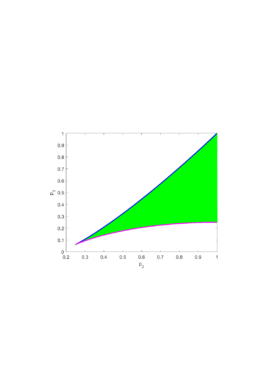
Figure 4: (Color Online) The PT-moment pair $(p_{2},p_{3})$ for X-state $\rho_{\mathrm{X}}$ falls within the green colored region. The upper blue curve and the lower magenta curve correspond to $\Phi_{4}^{\pm}(p_{2})$, respectively, where $p_{2}\in[\frac{1}{4},1]$.

4.2 multipartite system

In this subsection, we keep applying our results in Sec. 3 to further detect the entanglement of high-dimensional and multipartite states. Firstly, we consider a bipartite state $\rho$ supported on $\mathbb{C}^{2m}\otimes\mathbb{C}^{2n}$ with positive integers $m$ and $n$. We regard the system of $\rho$ consisted of four particles $A,B,C$ and $D$, where the dimensions of the four subsystems are $2,m,2,n$ respectively. By tracing out the subsystems $B$ and $D$, the reduced density operator $\rho_{AC}$ is a two-qubit state. Then we can experimentally detect the entanglement of $\rho_{AC}$ by measuring its PT-moments and using Theorem 3.1. If $\rho_{AC}$ is entangled then one can verify the entanglement of bipartite state $\rho_{AB:CD}$. Using a similar idea, one can detect the entanglement of a multiqubit or multipartite state.

For example, we consider the $n$-qubit mixed state which is the mixture of $n$-qubit GHZ and W states, namely

$$\rho^{(n)}=\lambda|\mathrm{G}\mathrm{H}\mathrm{Z}_{n}\rangle\!\langle\mathrm{G}\mathrm{H}\mathrm{Z}_{n}|+(1-\lambda)|\mathrm{W}_{n}\rangle\!\langle\mathrm{W}_{n}|,$$ (4.26)

where $\lambda\in[0,1]$, and

$$\begin{aligned} |\mathrm{G}\mathrm{H}\mathrm{Z}_{n}\rangle&=\tfrac{1}{\sqrt{2}}(|0\rangle^{\otimes n}+|1\rangle^{\otimes n}),\\ |\mathrm{W}_{n}\rangle&=\tfrac{1}{\sqrt{n}}(|0\cdots 01\rangle+|0\cdots 10\rangle+...+|10\cdots 0\rangle).\end{aligned}$$ (4.27)

Since $\rho^{(n)}$ is invariant under any permutation of the $n$ subsystems, by computing we obtain any bipartite reduced density operator of $\rho^{(n)}$ is

$$\rho^{(n)}_{AB}=\tfrac{\lambda}{2}(|00\rangle\!\langle 00|+|11\rangle\!\langle 11|)+\frac{1-\lambda}{n}(n-2)|00\rangle\!\langle 00|+\tfrac{1-\lambda}{n}(|01\rangle+|10\rangle)(\langle 01|+\langle 10|).$$ (4.28)

By straightforward computation, we obtain the four eigenvalues of its partial transpose are

$$\begin{aligned} &\tfrac{1-\lambda}{n},\quad\tfrac{1-\lambda}{n},\\ &\tfrac{1}{2}+\tfrac{(1-\lambda)(\sqrt{\delta_{n}}-2)}{2n},\\ &\tfrac{1}{2}-\tfrac{(1-\lambda)(\sqrt{\delta_{n}}+2)}{2n},\end{aligned}$$ (4.29)

where $\delta_{n}=n^{2}-4n+8\geqslant 4$. One can verify that the first three eigenvalues are always non-negative for any $n\geqslant 2$ when $\lambda\in[0,1]$. Hence, it follows from the PPT criterion that the two-qubit state $\rho^{(n)}_{AB}$ is entangled if and only if the last eigenvalue in Eq. (4.29) is negative. Specifically, by direct calculation we obtain that

• If $n=2$, then $0\leqslant\lambda<\frac{1}{2}$ corresponds to $\rho_{AB}$ being entangled;

• If $n>2$, then $0\leqslant\lambda<\frac{\delta_{n}-n\sqrt{\delta_{n}}+2n-4}{(n-2)^{2}}$ corresponds to $\rho_{AB}$ being entangled.

Note that $\lim\limits_{n\to\infty}\frac{\delta_{n}-n\sqrt{\delta_{n}}+2n-4}{(n-2)^{2}}=0$. It follows from Eq. (4.28) that entangled $\rho^{(n)}_{AB}$ asymptotically approaches to

$$\tfrac{n-2}{n}|00\rangle\!\langle 00|+\tfrac{1}{n}(|01\rangle+|10\rangle)(\langle 01|+\langle 10|)$$ (4.30)

as $n\to+\infty$. Furthermore, we can also conclude that the original $n$-qubit state $\rho^{(n)}$ in Eq. (4.26) which generates entangled two-qubit reduced density operators asymptotically approaches to $|\mathrm{W}_{n}\rangle\!\langle\mathrm{W}_{n}|$ as $n\to+\infty$.

Based on the four eigenvalues formulated in Eq. (4.29), we further calculate the PT-moments $p_{2}$ and $p_{3}$ as follows.

$$\begin{aligned} p_{2}(\lambda)=&\frac{h_{4,16}\lambda^{2}-2h_{6,16}\lambda+2h_{4,8}}{2n^{2}},\\ p_{3}(\lambda)=&\frac{6h_{4,8}\lambda^{3}+3(n-4)h_{6,12}\lambda^{2}-6(n-2)h_{6,12}\lambda+4(nh_{6,15}-12)}{4n^{3}},\end{aligned}$$ (4.31)

where $h_{x,y}:=n^{2}-xn+y$. We investigate the pairs of PT-moments $\left(p^{(n)}_{2}(\lambda),p^{(n)}_{3}(\lambda)\right)$, where $\lambda\in[0,1]$, similar to that in Sec. 4.1. We plot the parametric curves for $n=3,4,5,6$ in Fig. 5. From Fig. 5 we can see in which interval of $p_{2}$ the two-qubit reduced state $\rho^{(n)}_{AB}$ falls within the region of separable states defined by Theorem 3.1, and the same for the region of entangled states. Then for the interval of $p_{2}$ corresponding to entangled $\rho^{(n)}_{AB}$, we may experimentally verify the entanglement of the original $n$-qubit state $\rho^{(n)}$ in Eq. (4.26) because the PT-moments are measurable. Furthermore, since $\rho^{(n)}$ is a symmetric state, it is either genuinely entangled or fully separable. This means we present an operational way of verifying multiqubit genuine entanglement using Theorem 3.1.

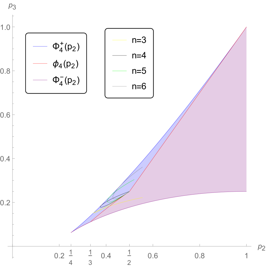
Figure 5: (Color Online) The PT-moment pair $\left(p^{(n)}_{2},p^{(n)}_{3}\right)$ of two-qubit state $\rho^{(n)}_{AB}$ in Eq. (4.28) for $n=3,4,5,6$.

5 Concluding remarks

In this short report, we derived an experimentally efficient separability criterion of two-qubit states based on the measurable PT-moments. Specifically, we concluded that a two-qubit state $\rho_{AB}$ is entangled if and only if the pair of its PT-moments $(p_{2},p_{3})$ belonging to the set $R_{\mathrm{ent}}$ defined by Eq. (3.5) following from Theorem 3.1. We also demonstrated our main result Theorem 3.1 geometrically in Fig 1. Our main contribution was determining the lowest curve $\Phi^{-}_{4}(p_{2})$ of $R_{\mathrm{ent}}$ in Fig 1. Then, in Sec. 4.1, we applied our main results to several widely-used families of two-qubit states such as the families of Werner states and Bell-diagonal states. We analytically identified the regions corresponding to the entangled states in these families. Moreover, we also extended our study on the two-qubit system to high-dimensional and multipartite systems in Sec 4.2. We mainly characterized the entanglement in the $n$-qubit state mixed by $n$-qubit GHZ and W states. Through identifying the region $R_{\mathrm{ent}}$ of the reduced two-qubit state in Fig. 5, we can experimentally verify the genuine entanglement of such multiqubit states. We hope the results obtained in this work can shed new light on some related problems in quantum information theory, such as to quantify both the values and numbers of the negative eigenvalues in the spectrum of $\rho_{AB}^{\Gamma}$.

Acknowledgments

The authors would like to thank the anonymous reviewers and the editor for their detailed and valuable comments which are very helpful to improve the standard of this paper. This work is supported by the NSF of China under Grant Nos. 11971140, 12171044 and 11871089, also supported by the National Key Research and Development Program of China under grant No. 2021YFA1000600.

Appendix A The proof of Theorem 3.1

Consider the objective function

$$f(x,y,z)=x^{3}+y^{3}+z^{3}+(1-x-y-z)^{3}\equiv p_{3},\quad(x,y,z)\in[0,1]^{3}$$

subjective to the constraints

$$x+y+z=s,\quad x^{2}+y^{2}+z^{2}+(1-x-y-z)^{2}=t\equiv p_{2}$$

where both parameters $s\in[1,\tfrac{3}{2}]$ and $t\in[\tfrac{1}{4},1]$ are fixed. Clearly $t-(1-s)^{2}\geqslant 0$ for $s\in[1,\tfrac{3}{2}]$ and $t\in[\tfrac{1}{4},1]$. Recall that

$$x^{3}+y^{3}+z^{3}-3xyz = (x+y+z)(x^{2}+y^{2}+z^{2}-xy-yz-zx)$$

$$= s\left[t-(1-s)^{2}-\frac{1}{2}(s^{2}+(1-s)^{2}-t)\right]$$

$$= \frac{1}{2}s\left(-4s^{2}+6s+3t-3\right)\geqslant 0.$$

Thus our objective function is reduced as

$$f(x,y,z)=3xyz+\frac{3}{2}s(-2s^{2}+4s+t-3)+1.$$

Denote by $g(x,y,z)=xyz$, where $(x,y,z)\in[0,1]^{3}$. Then

$$\min f(x,y,z)=3\min g(x,y,z)+\frac{3}{2}s(-2s^{2}+4s+t-3)+1$$

for given $s$ and $t$. Denote $M(t,s):=f_{\max}$ and $m(t,s):=f_{\min}$. Our problem becomes to consider the optimization of the function $g(x,y,z)$ subjective to the constraints:

$$x+y+z=s,\quad x^{2}+y^{2}+z^{2}=t-(1-s)^{2}.$$

Apparently the plain $x+y+z=s$ must intersect with the sphere $x^{2}+y^{2}+z^{2}=t-(1-s)^{2}$, which means that

$$\frac{\left\lvert\mspace{1.0mu}0+0+0-s\mspace{1.0mu}\right\rvert}{\sqrt{1^{2}+1^{2}+1^{2}}}\leqslant\sqrt{t-(1-s)^{2}}\Longleftrightarrow\frac{1}{3}<t\leqslant 1,1<s\leqslant\frac{3+\sqrt{3(4t-1)}}{4}\left(\leqslant\frac{3}{2}\right).$$

The plain $x+y+z=s$ is tangent to the sphere $x^{2}+y^{2}+z^{2}=t-(1-s)^{2}$ iff $s=\frac{3+\sqrt{3(4t-1)}}{4}$, where $t\in[\tfrac{1}{3},1]$. At this time,

$$x=y=z=\frac{s}{3}=\frac{3+\sqrt{3(4t-1)}}{12}.$$

Then

$$f(s/3,s/3,s/3) = 3g(s/3,s/3,s/3)+\frac{3(2-t)-2\sqrt{3(4t-1)}}{16}$$

$$= \frac{1}{24}\left[3(6t-1)-\sqrt{3}(4t-1)^{\frac{3}{2}}\right]\quad(t\in[\tfrac{1}{3},1]).$$

(i) If moreover $s>\sqrt{2}\sqrt{t-(1-s)^{2}}$ as well, i.e.,

$$\frac{s^{2}}{3}\leqslant t-(1-s)^{2}<\frac{s^{2}}{2}$$

that is, $(t,s)\in R_{1}\cup R_{2}$ where

$$R_{1} = \left\{(t,s):\frac{1}{3}\leqslant t<\frac{1}{2},1\leqslant s\leqslant\frac{3+\sqrt{3(4t-1)}}{4}\right\},$$

$$R_{2} = \left\{(t,s):\frac{1}{2}\leqslant t\leqslant 1,\frac{2+\sqrt{2(3t-1)}}{3}<s\leqslant\frac{3+\sqrt{3(4t-1)}}{4}\right\},$$

the plane $x+y+z=s$ must intersection with the sphere $x^{2}+y^{2}+z^{2}=t-(1-s)^{2}$ in a whole circle of the first octant; moreover this circle does not touch the three coordinate plains. By using Lagrange’s multiplier method, we let Lagrange’s function be

$$G(x,y,z,\mu,\nu)=xyz+\mu(x+y+z-s)+\nu(x^{2}+y^{2}+z^{2}-t+(1-s)^{2}).$$

Then

$$\begin{cases}\frac{\partial G}{\partial x}&=\mu+2\nu x+yz=0\\ \frac{\partial G}{\partial y}&=\mu+2\nu y+xz=0\\ \frac{\partial G}{\partial z}&=\mu+2\nu z+xy=0\\ \frac{\partial G}{\partial\mu}&=x+y+z-s=0\\ \frac{\partial G}{\partial\nu}&=x^{2}+y^{2}+z^{2}-t+(1-s)^{2}=0\end{cases}$$

Based on the previous three equations, we get that

$$\begin{cases}yz&=-\mu-2\nu x\\ xz&=-\mu-2\nu y\\ xy&=-\mu-2\nu z\\ \end{cases}\Longrightarrow\begin{cases}xyz&=-x(\mu+2\nu x)\\ xyz&=-y(\mu+2\nu y)\\ xyz&=-z(\mu+2\nu z)\\ \end{cases}$$

This implies that

$$2\nu x^{2}+\mu x=2\nu y^{2}+\mu y=2\nu z^{2}+\mu z.$$

Let $\varphi(r)=2\nu r^{2}+\mu r$ be a polynomial of 2nd degree in the argument $r$. Then the above fact means that $\varphi(x)=\varphi(y)=\varphi(z)$, i.e., $\varphi$ attains the same value at three points $x,y,z$. This indicates that at least two points of three points $x,y,z$ must be equal. Due to the symmetry of all permutations of $x,y,z$ for the objective function and constraints, without loss of generality, we assume that $x=y$. Thus

$$\begin{cases}x=2\nu\\ y=2\nu\\ z=s-4\nu\\ \mu=2\nu(2\nu-s)\end{cases}$$

Therefore we get that

$$\nu_{i}=\frac{2s+(-1)^{i}\sqrt{2(-4s^{2}+6s+3t-3)}}{12}\quad(i=1,2).$$

is the only two solutions allowing $(x,y,z)$ in the first orthant. Finally, we get two extremal points $(x_{i},y_{i},z_{i})(i=1,2)$, where

$$\begin{cases}x_{1}=&\frac{2s-\sqrt{2(-4s^{2}+6s+3t-3)}}{6}\\ y_{1}=&\frac{2s-\sqrt{2(-4s^{2}+6s+3t-3)}}{6}\\ z_{1}=&\frac{s+\sqrt{2(-4s^{2}+6s+3t-3)}}{3}\end{cases}\quad\text{and}\quad\begin{cases}x_{2}=&\frac{2s+\sqrt{2(-4s^{2}+6s+3t-3)}}{6}\\ y_{2}=&\frac{2s+\sqrt{2(-4s^{2}+6s+3t-3)}}{6}\\ z_{2}=&\frac{s-\sqrt{2(-4s^{2}+6s+3t-3)}}{3}\end{cases}$$

Note that $(x_{1},y_{1},z_{1})\in[0,1]^{3}$ if and only if $\frac{1}{3}\leqslant t\leqslant 1$ and $1\leqslant s\leqslant\frac{3+\sqrt{3(4t-1)}}{4}$; $(x_{2},y_{2},z_{2})\in(0,1)^{3}$ if and only if $(t,s)\in R_{1}\cup R_{2}$. In a word, when $(t,s)\in R_{1}\cup R_{2}$, we have two extremal points $(x_{i},y_{i},z_{i})(i=1,2)$. Thus $g_{i}=g(x_{i},y_{i},z_{i})$. The optimal values of $f$ are given by $f_{i}=x^{3}_{i}+y^{3}_{i}+z^{3}_{i}+(1-s)^{3}$, respectively, i.e.,

$$\begin{cases}M(t,s)=f_{1}=&\frac{1}{18}\left(-40s^{3}+90s^{2}+18st-72s+18+\sqrt{2}\left(-4s^{2}+6s+3t-3\right)^{\frac{3}{2}}\right)\\ m(t,s)=f_{2}=&\frac{1}{18}\left(-40s^{3}+90s^{2}+18st-72s+18-\sqrt{2}\left(-4s^{2}+6s+3t-3\right)^{\frac{3}{2}}\right)\end{cases}\quad(\forall(t,s)\in R_{1}\cup R_{2}).$$

(ii) If $s\leqslant\sqrt{2}\sqrt{t-(1-s)^{2}}$, i.e.,

$$t-(1-s)^{2}\geqslant\frac{s^{2}}{2}\left(\geqslant\frac{s^{2}}{3}\right)$$

that is, $(t,s)\in R_{3}=\left\{(t,s):\frac{1}{2}<t\leqslant 1,1\leqslant s\leqslant\frac{2+\sqrt{2(3t-1)}}{3}\right\}$, the plane $x+y+z=s$ must intersection with the sphere $x^{2}+y^{2}+z^{2}=t-(1-s)^{2}$ in three arcs separately of the first orthant; moreover such arcs touch the coordinate plains separately. Thus $g_{\min}=0$. Thus $f_{\min}=g_{\min}+\frac{3}{2}s(-2s^{2}+4s+t-3)+1=\frac{3}{2}s(-2s^{2}+4s+t-3)+1$. That is,

$$m(t,s)=\frac{3}{2}s(-2s^{2}+4s+t-3)+1\quad(\forall(t,s)\in R_{3}).$$

Using the analogous method as above, we get that $x=y=2\nu,z=s-4\nu$, where $\nu=\frac{2s-\sqrt{2(-4s^{2}+6s+3t-3)}}{12}$. Thus the maximal value of $f$ is still of the form

$$M(t,s)=\frac{1}{18}\left(-40s^{3}+90s^{2}+18st-72s+18+\sqrt{2}\left(-4s^{2}+6s+3t-3\right)^{\frac{3}{2}}\right)\quad(\forall(t,s)\in R_{3}).$$

In summary, we get that $p_{3}\geqslant m(t,s)$ where $(t,s)\in R:=R_{1}\cup R_{2}\cup R_{3}$, where

$$m(t,s)=\begin{cases}\frac{1}{18}\left[-40s^{3}+90s^{2}+18st-72s+18-\sqrt{2}\left(-4s^{2}+6s+3t-3\right)^{\frac{3}{2}}\right],&\text{if }\forall(t,s)\in R_{1}\cup R_{2};\\ \frac{3}{2}s(-2s^{2}+4s+t-3)+1,&\text{if }\forall(t,s)\in R_{3}.\end{cases}$$

In order to eliminate $s$, we make the optimization over the section for fixed $t$:

$$\max_{s\in R_{t}}M(t,s)\geqslant f(x,y,z)=p_{3}\geqslant\min_{s\in R_{t}}M(t,s)$$

$$\max_{s\in R_{t}}m(t,s)\geqslant f(x,y,z)=p_{3}\geqslant\min_{s\in R_{t}}m(t,s)$$

Note that

$$\min_{s\in R_{t}}M(t,s)=M\left(t,\frac{3+\sqrt{3(4t-1)}}{4}\right)=\frac{3(6t-1)-\sqrt{3}(4t-1)^{\frac{3}{2}}}{24}$$

$$\min_{s\in R_{t}}m(t,s)=m\left(t,\frac{3+\sqrt{3(4t-1)}}{4}\right)=\frac{3(6t-1)-\sqrt{3}(4t-1)^{\frac{3}{2}}}{24};$$

which means this value is a global minimal value, can be attained when $x=y=z$, as previously shown. We also see that

$$\max_{s\in R_{t}}M(t,s)=M(t,1)=\frac{2(9t-2)+\sqrt{2}(3t-1)^{\frac{3}{2}}}{18}$$

and

$$\max_{s\in(R_{1}\cup R_{2})_{t}}m(t,s) = \frac{2(9t-2)-\sqrt{2}(3t-1)^{\frac{3}{2}}}{18},\quad\frac{1}{3}<t<\frac{1}{2}$$

$$\max_{s\in(R_{3})_{t}}m(t,s) = m(t,1)=\frac{3t-1}{2},\quad\frac{1}{2}\leqslant t<1$$

that is,

$$\max_{s\in R_{t}}m(t,s) = \max\left\{\frac{2(9t-2)-\sqrt{2}(3t-1)^{\frac{3}{2}}}{18},\frac{3t-1}{2}\right\},\quad\quad\frac{1}{3}\leqslant t\leqslant 1.$$

Therefore

$$\min\left\{\max_{s\in R_{t}}M(t,s),\max_{s\in R_{t}}m(t,s)\right\}\geqslant f(x,y,z)=p_{3}\geqslant\max\left\{\min_{s\in R_{t}}M(t,s),\min_{s\in R_{t}}m(t,s)\right\}.$$

Here

$$\min\left\{\max_{s\in R_{t}}M(t,s),\max_{s\in R_{t}}m(t,s)\right\} = \max\left\{\frac{2(9t-2)-\sqrt{2}(3t-1)^{\frac{3}{2}}}{18},\frac{3t-1}{2}\right\},\quad\frac{1}{3}\leqslant t\leqslant 1$$

$$\max\left\{\min_{s\in R_{t}}M(t,s),\min_{s\in R_{t}}m(t,s)\right\} = \frac{3(6t-1)-\sqrt{3}(4t-1)^{\frac{3}{2}}}{24},\quad\frac{1}{3}\leqslant t\leqslant 1.$$

Now rewrite the above inequality by replacing $t$ as $p_{2}$. We get the desired:$\phi_{4}(p_{2})\geqslant p_{3}\geqslant\Phi^{-}_{4}(p_{2})$ for $p_{2}\in[\tfrac{1}{3},1]$. Due to the fact that $p_{3}=\phi_{4}(p_{2})$ for $p_{2}\in[\tfrac{1}{3},1]$ is compatible with $\rho_{AB}$ being separable, we finally obtain that

$$\phi_{4}(p_{2})>p_{3}\geqslant\Phi^{-}_{4}(p_{2}),\quad p_{2}\in(\tfrac{1}{3},1].$$

Appendix B The proof of inequality (4.8)

In fact, we note that the family of Werner states is a subset of the family of Bell-diagonal states. This indicates that

$$p_{3}\geqslant\phi^{-}_{4}(p_{2}).$$

This inequality is saturated for Werner states. Next, we show that $p_{3}\leqslant\Phi^{\mathrm{B}}_{4}(p_{2})$, where $p_{2}\in[\frac{1}{4},1]$.
(i) Assume that $p_{2}\in[\frac{1}{2},1]$ is fixed. Next we show that $p_{3}\leqslant\frac{1}{4}$. Recall that

$$p_{3}=\frac{1+3\sum^{3}_{i=1}t_{i}+6t_{1}t_{2}t_{3}}{16}=\frac{(6p_{2}-1)+3t_{1}t_{2}t_{3}}{8}.$$

Thus it suffices to show that $t_{1}t_{2}t_{3}\leqslant 1-2p_{2}(\leqslant 0)$ when $(t_{1},t_{2},t_{3})\in D_{\text{Bell}}$ and $p_{2}\in[\frac{1}{2},1]$. This amounts to do the following optimization problem: For $g(t_{1},t_{2},t_{3})=t_{1}t_{2}t_{3}$,

$$~{}~{}~{}~{}~{}~{}~{}\max g(t_{1},t_{2},t_{3})$$

subject to: $$(t_{1},t_{2},t_{3})\in D_{\text{Bell}}$$

$$t^{2}_{1}+t^{2}_{2}+t^{2}_{3}=4p_{2}-1\in[1,3].$$

Note that the sphere (which is denoted by $S$) $t^{2}_{1}+t^{2}_{2}+t^{2}_{3}=4p_{2}-1\in[1,3]$ intersect with the 3D region $D_{\text{Bell}}$ at four congruent pieces (outside of $D_{\text{Bellsep}}$), respectively, in 2nd, 4th, 5th, 7th orthant. See the following Figure 7.

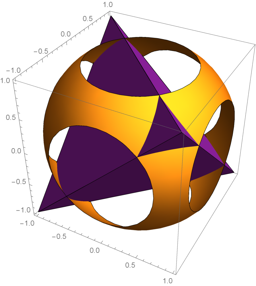
Figure 6: The optimization problem for Bell-diagonal states in the case where $p_{2}\in[\frac{1}{2},1]$.

For instance, we focus the pieces in the 4th orthant. When $t_{1}=1,t_{2}=-\sqrt{2p_{2}-1},t_{3}=\sqrt{2p_{2}-1}$, $g(t_{1},t_{2},t_{3})=1-2p_{2}$ attain its maximal value.
(ii) Assume that $p_{2}\in[\frac{1}{3},\frac{1}{2}]$ is fixed. This amounts to do the following optimization problem: For $g(t_{1},t_{2},t_{3})=t_{1}t_{2}t_{3}$,

$$~{}~{}~{}~{}~{}~{}~{}\max g(t_{1},t_{2},t_{3})$$

subject to: $$(t_{1},t_{2},t_{3})\in D_{\text{Bell}}$$

$$t^{2}_{1}+t^{2}_{2}+t^{2}_{3}=4p_{2}-1\in[\tfrac{1}{3},1].$$

Note that the sphere $S:t^{2}_{1}+t^{2}_{2}+t^{2}_{3}=4p_{2}-1\in[\tfrac{1}{3},1]$ intersect with $D_{\text{Bellsep}}$ at nontrivial nonempty set. As already obtained, $p_{3}$ will attain more larger values on separable states (corresponding to those points in $D_{\text{Bellsep}}$) versus entangled states (corresponding to those points in $D_{\text{Bell}}\backslash D_{\text{Bellsep}}$) when the purity $p_{2}$ is fixed. It suffices to consider the optimization problem:

$$~{}~{}~{}~{}~{}~{}~{}\max g(t_{1},t_{2},t_{3})$$

subject to: $$\left\lvert\mspace{1.0mu}t_{1}\mspace{1.0mu}\right\rvert+\left\lvert\mspace{1.0mu}t_{2}\mspace{1.0mu}\right\rvert+\left\lvert\mspace{1.0mu}t_{3}\mspace{1.0mu}\right\rvert=1,\text{ i.e., }(t_{1},t_{2},t_{3})\in\partial D_{\text{Bellsep}}$$

$$t^{2}_{1}+t^{2}_{2}+t^{2}_{3}=4p_{2}-1\in[\tfrac{1}{3},1].$$

In fact, by symmetry, we can further specialize the above boundary condition $(t_{1},t_{2},t_{3})\in\partial D_{\text{Bellsep}}$ to the case $t_{1}+t_{2}+t_{3}=1$, where $t_{i}\geqslant 0$ for $i=1,2,3$. Thus, for instance, $g(t_{1},t_{2},t_{3})$ attains its maximal value $\frac{(18p_{2}-1)+2\sqrt{2}(3p_{2}-1)^{\frac{3}{2}}}{36}$ when $t_{1}=t_{2}=\frac{1-\sqrt{2(3p_{2}-1)}}{3}$ and $t_{3}=\frac{1+2\sqrt{2(3p_{2}-1)}}{3}$, where $p_{2}\in[\frac{1}{3},\frac{1}{2}]$.
See the following Figure 7.

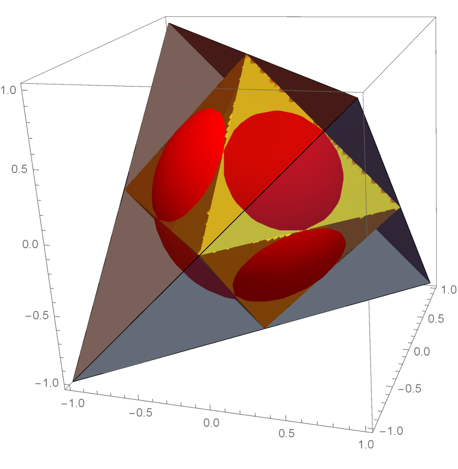
Figure 7: The optimization problem for Bell-diagonal states in the case where $p_{2}\in[\frac{1}{3},\frac{1}{2}]$.

(iii) Assume that $p_{2}\in[\frac{1}{4},\frac{1}{3}]$ is fixed. This amounts to do the following optimization problem: For $g(t_{1},t_{2},t_{3})=t_{1}t_{2}t_{3}$,

$$~{}~{}~{}~{}~{}~{}~{}\max g(t_{1},t_{2},t_{3})$$

subject to: $$(t_{1},t_{2},t_{3})\in D_{\text{Bell}}$$

$$t^{2}_{1}+t^{2}_{2}+t^{2}_{3}=4p_{2}-1\in[0,\tfrac{1}{3}].$$

Due to the fact that the whole sphere $S:t^{2}_{1}+t^{2}_{2}+t^{2}_{3}=4p_{2}-1\in[0,\tfrac{1}{3}]$ is contained in $D_{\text{Bellsep}}$. By using Lagrange’s multiplier method, we define Lagrange function

$$L(t_{1},t_{2},t_{3},\lambda):=t_{1}t_{2}t_{3}+\lambda(t^{2}_{1}+t^{2}_{2}+t^{2}_{3}-4p_{2}+1),$$

defined over the 1st orthant by symmetry. Then

$$\begin{cases}\frac{\partial L}{\partial t_{1}}&=t_{2}t_{3}+2\lambda t_{1}=0\\ \frac{\partial L}{\partial t_{2}}&=t_{1}t_{3}+2\lambda t_{2}=0\\ \frac{\partial L}{\partial t_{3}}&=t_{1}t_{2}+2\lambda t_{3}=0\\ \frac{\partial L}{\partial\lambda}&=t^{2}_{1}+t^{2}_{2}+t^{2}_{3}-4p_{2}+1=0\end{cases}$$

leads to the solution $t_{1}=t_{2}=t_{3}=\sqrt{\frac{4p_{2}-1}{3}}$, the extremal (maximal) point at which $p_{3}$ attains its maximal value

$$p_{3}=\frac{1+6\left(\sqrt{\frac{4p_{2}-1}{3}}\right)^{3}+3(4p_{2}-1)}{16}=\Phi^{+}_{4}(p_{2}).$$

In summary, this is the desired result: $\Phi^{-}_{4}(p_{2})\leqslant p_{3}\leqslant\Phi^{\textsf{B}}_{4}(p_{2})$, where

$$\Phi^{\textsf{B}}_{4}(p_{2})=\begin{cases}\Phi^{+}_{4}(p_{2}),&\text{if }p_{2}\in[\frac{1}{4},\frac{1}{3}],\\ \frac{(18p_{2}-1)+2\sqrt{2}(3p_{2}-1)^{\frac{3}{2}}}{36},&\text{if }p_{2}\in[\frac{1}{3},\frac{1}{2}],\\ \frac{1}{4},&\text{if }p_{2}\in[\frac{1}{2},1].\\ \end{cases}$$

References

- [1] C.H. Bennet and S.J. Wiesner, Communication via one- and two-particle operators on Einstein-Podolsky-Rosen states, Phys. Rev. Lett. 69, 2881(1992).
- [2] C.H. Bennet, G. Brassard, C. Crepeau, R. Jozsa, A. Peres, and W.K. Wootters, Teleporting an unknown quantum state via dual classical and Einstein-Podolsky-Rosen channels, Phys. Rev. Lett. 70, 1895 (1993).
- [3] D. Bouwmeester, J.W. Pan, K. Mattle, M. Eibl, H. Weinfurther, Z. Zeilinger, Experimental quantum teleportation, Nature 390, 575-579 (1997).
- [4] D. Deutsch, A. Ekert, R. Jozsa, C. Macchiavello, S. Popescu, and A. Sanpera, Quantum privacy amplification and the security of quantum cryptography over noisy channels, Phys. Rev. Lett. 77, 2818 (1996).
- [5] A. Peres, Separability criterion for density matrices, Phys. Rev. Lett. 77, 1413 (1996).
- [6] M. Horodecki, P. Horodecki, R. Horodecki, Separability of mixed states: necessary and sufficient conditions, Phys. Lett. A 223, 1-8 (1996).
- [7] B.M. Terhal, Bell inequalities and the separability criterion, Phys. Lett. A 271, 319 (2000).
- [8] M. Lewenstein, B. Kraus, J.I. Cirac, P. Horodecki, Optimization of entanglement witnesses, Phys. Rev. A 62, 052310 (2000).
- [9] L. Skowronek, K. Życzkowski, Positive maps, positive polynomials and entanglement witnesses, J. Phys. A : Math. Theor. 42, 325302 (2009).
- [10] D. Chrúsciński, J. Pytel, Constructing optimal entanglement witnesses. II. Witnessing entanglement in systems, Phys. Rev. A 82, 052310 (2010).
- [11] K.-C. Ha, S.-H. Kye, One-parameter family of indecomposable optimal entanglement witnesses arising from generalized Choi maps, Phys. Rev. A 84, 024302 (2011).
- [12] M.B. Plenio, Logarithmic negativity: a full entanglement monotone that is not convex, Phys. Rev. Lett. 95, 090503 (2005).
- [13] M. Horodecki, P. Horodecki, R. Horodecki, Asymptotic Manipulations of Entanglement Can Exhibit Genuine Irreversibility, Phys. Rev. Lett. 84, 4260(2000).
- [14] G. Vidal, R.R. Werner, Computable measure of entanglement, Phys. Rev. A 65, 032314 (2002).
- [15] K.M.R. Audenaert, M.B. Plenio, J. Eisert, Entanglement cost under positive-partial-transpose-preserving operations, Phys. Rev. Lett. 90, 027901 (2003).
- [16] X-D. Yu, S. Imai, O. Gühne, Optimal entanglement certification from moments of the partial transpose, Phys. Rev. Lett. 127, 060504 (2021).
- [17] P. Liu, Z. Liu, S. Chen, X. Ma, Fundamental Limitation on the Detectability of Entanglement, Phys. Rev. Lett. 129, 230503 (2022).
- [18] A. Elben, R. Kueng, H-Y.R. Huang, R. van Bijnen, C. Kokail, M. Dalmonte, P. Calabrese, B. Kraus, J. Preskill,P. Zoller, and B. Vermersch, Mixed-state entanglement from local randomized measurements, Phys. Rev. Lett. 125, 200501 (2020).
- [19] H.-Y. Huang, R. Kueng, and J. Preskill, Predicting many properties of a quantum system from very few measurements, Nature Phys. 16, 1050 (2020).
- [20] J. Gray, L. Banchi, A. Bayat, and S. Bose, Machine-learning-assisted many-body entanglement measurement, Phys. Rev. Lett. 121, 150503 (2018).
- [21] Y. Zhou, P. Zeng, and Z. Liu, Single-copies estimation of entanglement negativity, Phys. Rev. Lett. 125, 200502 (2020).
- [22] Z. Liu, Y. Tang, H. Dai, P. Liu, S. Chen, X. Ma, Detecting entanglement in quantum many-body systems via permutation moments, Phys. Rev. Lett. 129, 260501 (2022).
- [23] R. Simon, Peres-Horodecki Separability Criterion for Continuous Variable Systems, Phys. Rev. Lett. 84, 2726 (2000).
- [24] L.-M. Duan, G. Giedke, J.I. Cirac, P. Zoller, Inseparability Criterion for Continuous Variable Systems, Phys. Rev. Lett. 84, 2722 (2000).
- [25] S. Mancini, V. Giovannetti, D. Vitalli, P. Tombesi, Phys. Rev. Lett. 88, 120401 (2002).
- [26] G.S. Agarwal, A. Biswas, Quantitative measures of entanglement in pair-coherent states, J. Opt. B: Quantum Semiclassical Opt. 7, 350 (2005).
- [27] E. Shchukin, W. Vogel, Inseparability Criteria for Continuous Bipartite Quantum States, Phys. Rev. Lett. 95, 230502 (2005).
- [28] A. Miranowicz, M. Piani, Comment on "Inseparability Criteria for Continuous Bipartite Quantum States", Phys. Rev. Lett. 97, 058901 (2006).
- [29] W. Vogel, Nonclassical Correlation Properties of Radiation Fields, Phys. Rev. Lett. 100, 013605 (2008).
- [30] A. Miranowicz, M. Bartkowiak, X. Wang, Y-x. Liu, F. Nori, Testing nonclassicality in multimode fields: A unified derivation of classical inequalities, Phys. Rev. A 82, 013824 (2010).
- [31] T.-C. Wei, K. Nemoto, P.M. Goldbart, P.G. Kwiat, W.J. Munro, F. Verstraete, Maximal entanglement versus entropy for mixed quantum states, Phys. Rev. A 67, 022110 (2003).
- [32] K. Bartkiewicz, B. Horst, K. Lemr, A. Miranowicz, Entanglement estimation from Bell inequality violation, Phys. Rev. A 88, 052105 (2013).
- [33] B. Horst, K. Bartkiewicz, A. Miranowicz, Two-qubit mixed states more entangled than pure states: Comparison of the relative entropy of entanglement for a given nonlocality, Phys. Rev. A 87, 042108 (2013).
- [34] K. Bartkiewicz, J. Beran, K. Lemr, M. Norek, A. Miranowicz, Quantifying entanglement of a two-qubit system via measurable and invariant moments of its partially transposed density matrix, Phys. Rev. A 91, 022323 (2015).
- [35] S. Rana, Negative eigenvalues of partial transposition of arbitrary bipartite states, Phys. Rev. A 87, 054301 (2013).
- [36] N. Johnston, Separability from spectrum for qubit-qudit states, Phys. Rev. A 88, 062330 (2013).
- [37] Y. Shen, L. Chen, L-J. Zhao, Inertias of entanglement witnesses, J. Phys. A : Math. Theor. 53, 485302 (2020).
- [38] J. Duan, L. Zhang, Q. Qian, and S-M. Fei, A characterization of maximally entangled two-qubit states, Entropy 24(2), 247 (2022).
- [39] A.K. Ekert, C.M. Alves, D.K.L. Oi, M. Horodecki, P. Horodecki, and L.C. Kwek, Direct estimations of linear and nonlinear functionals of a quantum state, Phys. Rev. Lett. 88, 217901 (2002).
- [40] R. Horodecki, M. Horodecki, Information-theoretic aspects of inseparability of mixed states, Phys. Rev. A 54(3), 1838 (1996).
- [41] A. Lovas, A. Andai, Invariance of separability probability over reduced states in bipartite systems, J. Phys. A : Math. Theor. 50, 295303 (2017).
- [42] R.F. Werner, Quantum states with Einstein-Podolsky-Rosen correlations admitting a hidden-variable model, Phys. Rev. A 40 4277 (1989).
- [43] D.P. DiVincenzo, P.W. Shor, J.A. Smolin, B.M. Terhal, A.V. Thapliyal, Phys. Rev. A 61, 062312 (2000).
- [44] M.J. Zhao, R. Pereira, T.Ma, and S.M. Fei, Coherence of assistanc and assisted maximally coherent states, Sci. Rep. 11, 5935 (2021).
- [45] S. Luo, Quantum discord for two-qubit systems, Phys. Rev. A 77, 042303 (2008).
- [46] M. Ali, Distillability sudden death in qutrit-qutrit systems under global and multilocal dephasing, Phys. Rev. A 81, 042303 (2010).
- [47] A. Maldonado-Trapp, A. Hu, and L. Roa, Analytical solutions and criteria for the quantum discord of two-qubit X-states, Quantum Inf. Process. 14, 6 (2015).
- [48] B.L. Ye, Y.K. Wang, and S.M. Fei, One-way quantum deficit and decoherence for two-qubit X sates, Int. J. Thero. Phys. 55, 2237-2246 (2016).
- [49] Y.K. Wang, N. Jing, S.-M. Fei, Z.X. Wang, J.P. Gao, and H. Fan, One-way deficit of two qubit X states, Quantum Inf. Process. 14, 2487-2497 (2015).
- [50] M.J. Zhao, M. Teng, Z. Wang, S.-M. Fei, and R. Pereira, Coherence concurrence for X states, Quantum Inf. Process. 19, 104 (2020).
- [51] Y. Wang, M.J. Zhao, T.G. Zhang, The Transformation From Pure States to X States Under Incoherent Operations, Int. J. Theo. Phys. 60, 2976-2985 (2021).