Species of structure and physical dimensions

Abstract

This study addresses the often underestimated importance of physical dimensions and units in the formal reconstruction of physical theories, focusing on structuralist approaches that use the concept of “species of structure" as a meta-mathematical tool. We are pursuing an approach that goes back to a suggestion by T. Tao. It involves the representation of fundamental physical quantities by one-dimensional real ordered vector spaces, while derived quantities are formulated using concepts from linear algebra, e. g. tensor products and dual spaces. As an introduction, the theory of Ohm’s law is considered. We then formulate a reconstruction of the calculus of physical dimensions, including Buckingham’s $\Pi$-theorem. Furthermore, an application of this method to the Newtonian theory of gravitating systems consisting of point particles is demonstrated, emphasizing the role of the automorphism group.

I Introduction

Physical quantities are not simply numbers, but have a physical dimension and can be represented accordingly by products of numbers with physical units. This is a fundamental fact that is already taught to schoolchildren in physics lessons. It is therefore surprising that this topic hardly plays a role in the formal reconstruction of physical theories. Perhaps it is considered all too trivial, as it has been known since school.

In the following, we will limit ourselves to approaches to the reconstruction of physical theories that can be described as “structuralistic” in a broad sense, see S24 . In the corresponding main works we find on the one hand indications that in the reconstructions of physical theories “space" and “time" cannot simply be modeled by ${\mathbb{R}}^{3}$ and ${\mathbb{R}}$, see L90 , p. 88, and BMS87 , p. 30 ff. On the other hand, the special character of dimensional quantities is not consistently taken into account, for example when introducing masses as positive real numbers, see L90 , p. 90, or BMS87 , p. 31.

What the structuralistic approaches have in common is that they use the meta-mathematical tool of so-called “species of structure" for the reconstruction of physical theories. The concept of “species of structure" is initially based on the insight, which goes back to N. Bourbaki, that mathematical theories such as "Lie groups" or "linear algebra" can be understood as theories of certain species of structure. This concept develops its real effectiveness when it is extended to relationships between species of structure, which will, however, not play a role in this paper. In the context of physics, it is now crucial to realize that physics not only makes use of mathematics in a general sense, but that to every physical theory $T$ can be assigned a species of structure $\Sigma$. Among other things, $\Sigma$ contains a collection of base sets, some of which can be given a physical meaning. Obviously, one can calculate with physical quantities, you can add them and you can multiply and divide them thus forming new quantities. Therefore they should belong to the mathematical part of $T$ and occur in $\Sigma$. It would therefore make sense to choose some of the basic quantities as ranges of physical quantities. A representative of the opposite position could argue that physical quantities and units belong to the practice of the experimental physicist who deals with measuring instruments, and only the pure numerical values are relevant for a theoretical treatment and therefore also for the reconstruction of physical theories.

But this position fails to recognize that there is no fundamental distinction between "proper theories" and "measurement theories" and that the latter may also be included in the reconstruction. There are also technical problems if, for example, the set of positions of a particle is represented by an auxiliary base set such as ${\mathbb{R}}^{3}$ in $\Sigma$. The automorphisms of the mathematical objects described by a species of structure leave the auxiliary base sets fixed; it would therefore not be possible to investigate symmetries of physical space as automorphisms of $\Sigma$.

Therefore, in this paper we take the position that physical quantities must be represented by base sets of $\Sigma$ and suitable structural elements and axioms and make suggestions for this. Ranges of physical quantities are represented by one-dimensional ordered real vector spaces and the calculus of physical quantities will be reconstructed by employing the mathematical concepts from linear algebra of tensor products of vector spaces and the dual of a vector space. This approach was suggested several years ago in a weblog by Terence Tao T13 . The physical calculus of units and the arithmetic of physical quantities should result from this representation and not be postulated separately. However, we cannot present a complete theory of physical dimensions here, but must limit ourselves to examples.

At first glance, it looks as if this approach ensures that the ban on adding physical quantities of different dimensions, which is familiar from physics lessons, is observed. The sum of elements of different vector spaces is simply not mathematically defined. In reality, however, the situation is somewhat more complicated, partially due to the existence of dimensional constants of nature, see section IV.

In Section II we consider a physical theory designated to formulate Ohm’s law. As simple as this theory is, it already illustrates a fundamental issue in the theory of physical quantities, namely how a new quantity with the derived dimension “resistance" can be obtained from two fundamental quantities such as “voltage" and “current" on the basis of a law, in this case Ohm’s law.

The first version of Ohm’s theory $TO_{1}$ is formulated in Section II.1. It essentially contains three basic sets representing “resistors", “voltmeters" and “ampere meters" and a structural element representing a set of measurements on these devices. The two ranges ${\mathcal{U}}$ and ${\mathcal{I}}$ of the physical quantities “voltage" resp. ‘current" are defined as suitable equivalence classes and equipped with the structure of one-dimensional real vector spaces. In a way, we are thus moving backwards in the history of physics and reconstructing the invention of dimensional quantities, which considerably simplifies the earlier way of only talking about ratios between quantities.

In Section II.2 a second version $TO_{2}$ is considered where the two spaces ${\mathcal{U}}$ and ${\mathcal{I}}$ are base set from the outset and Ohm’s law is formulated by simultaneously introducing the derived quantity “resistance" with range ${\mathcal{U}}\otimes{\mathcal{I}}^{\ast}$.

This approach is used in Section III to sketch the general calculus of physical quantities and to make a connection to the well-known $\Pi$-theorem. Also $3$-dimensional vector quantities are considered in Section III.2 since they are required for Section V. The next Section IV contains a informal account of the notion of “species of structure" and an example of how it would be defined for Ohm’s theory of Section II.2. In Section V we outline a “real" physical theory, namely Newton’s theory $TN$ of $N$ gravitationally interacting point particles using the formalism developed in Section III. There is some similarity between Ohm’s law $U=R\,I$ and the equation of motion in $TN$, saying that the force on the $i$th particle is the product of $\Gamma$ times the sum of the contributions due to attractions from the other particles. But in this case the gravitational constant $\Gamma$ is universal and could, in principle, be used to reduce the number of fundamental quantities.

We close with a summary and outlook in Section VI. Appendix A contains a proof of the equivalence between an “abstract" and a “parametric" form of Ohm’s law. In Appendix B we recapitulate an axiomatic characterization of positive domains and their embedding into ranges of physical quantities. The appendix C contains a proposal for a definition of rational powers of physical quantities, which, however, are not needed for the rest of the paper. Finally, the Appendix D contains a heuristic account of the mathematical notions of tensor products and dual spaces that are crucial for the present reconstruction of the dimensional calculus.

II Ohm’s law $U=R\,I$

We consider a highly simplified physical toy theory, which is essentially built around Ohm’s law. This theory will be used to explain the basic definitions for "ranges of physical quantities".

II.1 Theory $TO_{1}$

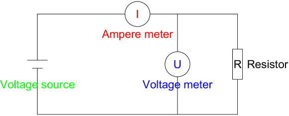
Figure 1: Schematic sketch of an electrical circuit for carrying out measurements to confirm Ohm’s law.

We consider a set of electrical resistors that are produced using some established methods, which is represented by a base set ${\sf R}$. Various voltages are applied to these resistors, which are measured together with the resulting electrical currents, see Figure 1. Each of these measurements can be represented by a 6-tuple $(R,S,U,u,I,i)$, where $R\in{\sf R}$, $S\in{\mathcal{S}}$, $U\in{\mathbb{U}}$, $I\in{\mathbb{I}}$, and $u,i\in{\mathbb{R}}_{>0}$. Here we have introduced further base sets ${\mathcal{S}}$ for voltage sources, ${\mathbb{U}}$ for voltmeters and ${\mathbb{I}}$ for ampere meters. The latter are measuring devices equipped with a scale from which one can read off the positive numbers occurring in the 6-tuple, but they are not yet gauged. The set of all possible measurements will be mathematically represented by the subset

$$\Gamma\subset{\sf R}\times{\mathcal{S}}\times{\mathbb{U}}\times{\mathbb{R}}\times{\mathbb{I}}\times{\mathbb{R}}\;.$$ (1)

The experiments suggest the following theory, which will be sketched in an informal way. If a resistor is connected to a voltage source then the readings $u_{1},u_{2}$ of two voltmeters $U_{1},U_{2}$ will be always proportional with a positive proportionality factor $u_{1}=\lambda_{u}(U_{1},U_{2})\,u_{2}$ that is the same for all experiments with different resistors and different voltage sources. It follows under mild assumptions that for all $U_{1},U_{2}.U_{3}\in{\mathbb{U}}$:

$$\lambda_{u}(U_{1},U_{1}) = 1,$$ (2)

$$\lambda_{u}(U_{1},U_{2})\,\lambda_{u}(U_{2},U_{1}) = 1,$$ (3)

$$\lambda_{u}(U_{1},U_{2})\,\lambda_{u}(U_{2},U_{3}) = \lambda_{u}(U_{2},U_{3})\;.$$ (4)

This implies that the relation

$$(U_{1},u_{1})\sim(U_{2},u_{2})\stackrel{{\scriptstyle\rm def}}{{\Leftrightarrow}}u_{1}=\lambda_{u}(U_{1},U_{2})\,u_{2}$$ (5)

will be an equivalence relation on ${\mathbb{U}}\times{\mathbb{R}}_{>0}$. The corresponding set of equivalence classes will be denoted by

$${\mathcal{U}}_{>0}:=\left({\mathbb{U}}\times{\mathbb{R}}_{>0}\right)_{\sim}\;,$$ (6)

and will be called the “positive range of voltages". The addition of two voltages can be defined by

$$\left[(U_{1},u_{1})\right]_{\sim}+\left[(U_{2},u_{2})\right]_{\sim}:=\left[(U_{1},u_{1}+\lambda_{u}(U_{1},U_{2})u_{2})\right]_{\sim}\;,$$ (7)

and the multiplication of a voltage with a positive real $x\in{\mathbb{R}}_{>0}$ by

$$x\cdot\left[(U,u)\right]_{\sim}:=\left[(U,x\cdot u)\right]_{\sim}\;.$$ (8)

Upon introducing an arbitrary “voltage unit" $U_{0}\in{\mathbb{U}}$ the range of positive voltages can be mapped onto ${\mathbb{R}}_{>0}$ by the map

$$f_{0}:\left[\left(U,u\right)\right]_{\sim}\mapsto\lambda_{u}(U_{0},U)\,u\;,$$ (9)

where (2) - (4) suffice to show that $f_{0}$ does not depend on the representative of the equivalence class and will be injective. The usual, albeit unphysical assumptions of arbitrary large possible voltages allow to extend $f_{0}$ to a bijective map

$$f_{0}:{\mathcal{U}}_{>0}\rightarrow{\mathbb{R}}_{>0}\;.$$ (10)

Then it can be shown that $f_{0}$ will be an isomorphism $f_{0}:\left({\mathcal{U}}_{>0},+,\cdot\right)\rightarrow\left({\mathbb{R}}_{>0},+,\cdot\right)$.

It is well-know that $({\mathbb{R}}_{>0},+,\cdot)$ can be embedded into the field $({\mathbb{R}},+,\cdot)$, where the real numbers can be constructed as equivalence classes of pairs of positive reals. Analogously, $\left({\mathcal{U}}_{>0},+,\cdot\right)$ can be embedded into a one-dimensional, real ordered vector space $\left({\mathcal{U}},+,\cdot,<\right)$, see Proposition 1 in the Appendix B. We stress that the $\cdot$ in $\left({\mathcal{U}},+,\cdot,<\right)$ denotes the external multiplication with real numbers.

It is clear how to apply the foregoing considerations to the analogous case of ampere meters to obtain the range of the physical quantity “current"

$${\mathcal{I}}_{>0}\subset{\mathcal{I}}\;.$$ (11)

The extension of the range of positive quantities to the range of signed quantities is mathematically convenient but does not imply that the negative quantities have any physical meaning. In the case of voltages or currents it is possible to extend the physical meaning to negative values, but this cannot be assumed generally.

II.2 Theory $TO_{2}$

For the next steps in the reconstruction of Ohm’s theory we do not need the full content of the theory $TO_{1}$ but will abstract from the reference to voltmeters and ampere meters and only consider the physical quantities obtained by the measurements. Moreover, we identify two resistors $R_{1},R_{2}$ iff they always yield the same values in measurements, i. e., iff $(R_{1},S,U,u,I,i)\in\Gamma\Leftrightarrow(R_{2},S,U,u,I,i)\in\Gamma$ for all $S\in{\mathcal{S}},U\in{\mathbb{U}},u\in{\mathbb{R}},I\in{\mathbb{I}},i\in{\mathbb{R}}$. The corresponding set of equivalence classes will be denoted by ${\mathcal{R}}$ and its elements $R\in{\mathcal{R}}$ will be again called “resistors". This formulation constitutes the theory $TO_{2}$. Its base sets are the set of resistors ${\mathcal{R}}$ and the two ranges of voltages ${\mathcal{U}}$ and currents ${\mathcal{I}}$. As explained in Section II.1, ${\mathcal{U}}$ and ${\mathcal{I}}$ are one-dimensional, real, ordered vector spaces. Physical units such as “Volt" or “Ampère" are positive bases in ${\mathcal{U}}$ or, resp. , ${\mathcal{I}}$. They consist of a singleton since the spaces are one-dimensional. A physical quantity like “voltage" can hence be written in the familiar way as a positive number times a physical unit.

The subset (1) will be replaced by

$$\gamma\subset{\mathcal{R}}\times{\mathcal{U}}\times{\mathcal{I}}\;,$$ (12)

with the meaning of $(R,U,I)\in\gamma$ that, when connecting the resistor $R$ to some voltage source, the voltage $U$ and the current $I$ has been measured. We stress again that $U$ and $I$ are not real numbers but physical quantities of different dimensions.

We now turn to the problem of how to formulate the experimental finding that $U$ is proportional to $I$ in different experiments with the same resistor $R$. To this end we consider linear mappings $m:{\mathcal{I}}\rightarrow{\mathcal{U}}$. The space of these mappings is again one-dimensional and can be identified with ${\mathcal{U}}\otimes{\mathcal{I}}^{\ast}$, where $\otimes$ denotes the tensor product of vector spaces and ${\mathcal{I}}^{\ast}$ the dual vector space defined as the space of linear mappings $\imath:{\mathcal{I}}\rightarrow{\mathbb{R}}$. In linear algebra this is the usual identification of second rank tensors possessing one covariant index and one contravariant index with the matrix of a linear map. Because of the one-dimensionality, the elements of ${\mathcal{U}}\otimes{\mathcal{I}}^{\ast}$ can be written in the form $U\otimes\imath$, with $U\in{\mathcal{U}}$ and $\imath\in{\mathcal{I}}^{\ast}$. This representation is only unique up to the scale transformation $U\mapsto\alpha U$ and $\imath\mapsto\frac{1}{\alpha}\imath$ for arbitrary $\alpha\in{\mathbb{R}},\,\alpha\neq 0$.

In order to make the identification of ${\mathcal{U}}\otimes{\mathcal{I}}^{\ast}$ with the graph of a linear map explicit, we define

$${\rm graph}:{\mathcal{U}}\otimes{\mathcal{I}}^{\ast}\rightarrow{\mathcal{P}}\left({\mathcal{U}}\times{\mathcal{I}}\right)$$ (13)

by

$$\left(U,I\right)\in{\rm graph}\left(U_{0}\otimes\jmath_{0}\right)\;\Leftrightarrow\;U=U_{0}\;\jmath_{0}(I)\;.$$ (14)

With this preparation we will formulate the main axiom of $TO_{2}$:

Axiom 1

For all $R\in{\mathcal{R}}$ there exists a $U_{1}\otimes\imath_{1}\in\left({\mathcal{U}}\otimes{\mathcal{I}}^{\ast}\right)_{>0}$ such that

$$\left\{(U,I)\left.\right|(R,U,I)\in\gamma\right\}={\rm graph}\left(U_{1}\otimes\imath_{1},\right)\;.$$ (15)

This axiom says that, first, for a fixed resistor $R$, the measured values of $(U,I)$ lie on a line passing through the origin. Second, the slope $\frac{\Delta U}{\Delta I}$ of the line has the value $U_{1}\otimes\imath_{1}\in{\mathcal{U}}\otimes{\mathcal{I}}^{\ast}$. This slope is not a real number but an element of ${\mathcal{U}}\otimes{\mathcal{I}}^{\ast}$, which is an ordered, linear one-dimensional vector space that can be viewed as a derived range of a new physical quantity. This quantity is, of course, the electrical resistance, and Axiom 1 enables us to define abijection

$$\rho:{\mathcal{R}}\rightarrow\left({\mathcal{U}}\otimes{\mathcal{I}}^{\ast}\right)_{>0}\;,$$ (16)

that assigns a resistance to each resistor and endows ${\mathcal{R}}$ with the structure of a positive range in the sense of the Appendix B. Introducing positive basis vectors, say, ${\rm Volt}\in{\mathcal{U}}$ and $\mbox{Amp\`{e}re}\in{\mathcal{I}}$ we obtain, first, a dual basis $\mbox{Amp\`{e}re}^{-1}\in{\mathcal{I}}^{\ast}$ defined by $\mbox{Amp\`{e}re}^{-1}(\mbox{Amp\`{e}re})=1$ and, second, a product basis ${\rm Ohm}:={\rm Volt}\otimes\mbox{Amp\`{e}re}^{-1}\in{\mathcal{U}}\otimes{\mathcal{I}}^{\ast}$.

One can given another formulation of Axiom 1 in a style closer to what T. Tao T13 calls the “parametric approach":

Axiom 2

For all $R\in{\mathcal{R}}$ and all $U_{0}\in{\mathcal{U}}_{>0},\,I_{0}\in{\mathcal{I}}_{>0}$ there exists an $r\in{\mathbb{R}}_{>0}$ such that for all $u,i\in{\mathbb{R}}_{>0}$

$$\left(R,u\,U_{0},i\,I_{0}\right)\in\gamma\Leftrightarrow u=r\,i\;.$$ (17)

Here the traditional form of Ohm’s law appears in (17) as $u=r\,i$. The equivalence of Axiom 1 and Axiom 2 is shown in the Appendix A.

The formalism of dual spaces and tensor product spaces of one-dimensional real vector spaces thus allows a reconstruction of the familiar calculus of multiplication and division of physical units. This is discussed in more detail in the next section.

III Calculus of physical quantities and Buckingham’s $\Pi$-theorem

III.1 Scalar quantities

Generalizing the situation of the theory $TO_{2}$ sketched in the preceding section, we consider the case where a physical theory contains $N$ ranges of fundamental scalar physical quantities ${\mathcal{R}}_{i}\,\;i=1,\ldots,N$. These are assumed to be equipped with the structure of one-dimensional ordered, real vector spaces. The order is given by a subset of the positive quantities ${\mathcal{R}}_{i,>0}$, as in the previous section.

In Section II we have given an example of how the fundamental quantities and their structure can be derived physically. For other cases it is assumed that there are analogous derivations. A general scheme for such derivations is known as the “representational theory of measurement" M87 , see also the theory of measurement presented in the three volumes of KLST71 , appendix A of F07 and section 2.4 of B15 .

From these fundamental quantities one can construct derived quantities just as the quantity “resistance" from the fundamental quantities “voltage" and “current" in the preceding section. For this construction we will use repeatedly the tensor product ${\mathcal{R}}_{i}\otimes{\mathcal{R}}_{j}$ and the dual space ${\mathcal{R}}_{i}^{\ast}$. ${\mathcal{R}}_{i}^{\ast}$ is also a one-dimensional ordered, real vector space if we define

$$\mbox{For all}\;\rho\in{\mathcal{R}}_{i}^{\ast}:\;\rho>0\quad\stackrel{{\scriptstyle\rm def}}{{\Leftrightarrow}}\quad\rho(R)>0\;\mbox{for all}\;R\in R_{i,>0}\;.$$ (18)

In the general case we have to take account of two complications. First, we will not distinguish between the two quantities ${\mathcal{R}}_{i}\otimes{\mathcal{R}}_{j}$ and ${\mathcal{R}}_{j}\otimes{\mathcal{R}}_{i}$. More generally, $k$-fold tensor products of fundamental quantities have to be distinguished only modulo permutations. Second, physical units can be cancelled. This means for our formalism that the one-dimensional real vector space ${\mathcal{R}}_{i}\otimes{\mathcal{R}}_{i}^{\ast}$ has to be identified with ${\mathbb{R}}$ by means of the “canonical" isomorphism ${\sf C}:{\mathcal{R}}_{i}\otimes{\mathcal{R}}_{i}^{\ast}\rightarrow{\mathbb{R}}$ (${\sf C}$ for cancellation) defined by

$${\sf C}(R\otimes\rho):=\rho(R)\;,$$ (19)

where $R\in{\mathcal{R}}_{i},\,\rho\in{\mathcal{R}}_{i}^{\ast}$ and the definition (19) does not depend on the chosen sclase factors, i. e., ${\sf C}\left(\alpha R\otimes\frac{1}{\alpha}\rho\right)={\sf C}(R\otimes\rho),\,\alpha>0$. This canonical isomorphism can be easily extended to multiple tensor products of ${\mathcal{R}}_{i}$ and ${\mathcal{R}}_{i}^{\ast}$. To simplify the notation we will write

$${\mathcal{R}}_{i}^{\ell} := \underbrace{{\mathcal{R}}_{i}\otimes\ldots\otimes{\mathcal{R}}_{i}}_{\ell\,{\rm factors}}\;,$$ (20)

$${\mathcal{R}}_{i,>0}^{\ell} := \underbrace{{\mathcal{R}}_{i,>0}\otimes\ldots\otimes{\mathcal{R}}_{i,>0}}_{\ell\,{\rm factors}}\;,$$ (21)

and

$${\mathcal{R}}_{i}^{-k} := \underbrace{{\mathcal{R}}_{i}^{\ast}\otimes\ldots\otimes{\mathcal{R}}_{i}^{\ast}}_{k\,{\rm factors}}\;,$$ (22)

$${\mathcal{R}}_{i,>0}^{-k} := \underbrace{{\mathcal{R}}_{i,>0}^{\ast}\otimes\ldots\otimes{\mathcal{R}}_{i,>0}^{\ast}}_{k\,{\rm factors}}\;.$$ (23)

Then the extension of ${\sf C}$ can be written compactly as

$${\sf C}:{\mathcal{R}}_{i}^{\ell}\otimes{\mathcal{R}}_{i}^{-k}\rightarrow{\mathcal{R}}_{i}^{\ell-k}\;,$$ (24)

for arbitrary natural numbers $\ell,k$ and setting ${\mathcal{R}}_{i}^{0}:={\mathbb{R}}$. The further extension to the case of integers $\ell,k$ is obvious.

According to the preceding remarks and definitions we define a “derived quantity" $Q^{({\mathbf{n}})}$ as an element of the one-dimensional real space

$${\mathcal{R}}^{({\mathbf{n}})}:=\bigotimes_{i=1}^{N}{\mathcal{R}}_{i}^{n(i)}\;,$$ (25)

where ${\mathbf{n}}=(n(1),\ldots,n(N))$ is an $N$-tuple of integers, i. e., ${\mathbf{n}}\in{\mathbb{Z}}^{N}$. Thus the range ${\mathcal{R}}^{(n)}$ of a derived quantity is completely characterized by the $N$-tuple ${\mathbf{n}}$. Fundamental quantities $R_{j}$ are special cases of derived quantities obtained by setting $n(i)=\delta_{ij}$.

The order of ${\mathcal{R}}^{({\mathbf{n}})}$ is given by the subset of positive quantities

$${\mathcal{R}}^{({\mathbf{n}})}_{>0}:=\bigotimes_{i=1}^{N}{\mathcal{R}}_{i,>0}^{n(i)}\;.$$ (26)

Next we define the product of two derived quantities $Q^{({\mathbf{n}})},Q^{({\mathbf{m}})}$.

$$Q^{({\mathbf{n}})}\,Q^{({\mathbf{m}})}:=\bigotimes_{i=1}^{N}{\sf C}\left(R_{i}^{n(i)}\otimes R_{i}^{m(i)}\right)\in\bigotimes_{i=1}^{N}{\mathcal{R}}_{i}^{(n+m)(i)}={\mathcal{R}}^{({\mathbf{n}}+{\mathbf{m}})}\;.$$ (27)

In special cases the product of quantities is simply the tensor product, but in general the cancellation operator ${\sf C}$ is additionally involved.

The inverse of a derived quantity will be defined in three steps. First, we define the inverse $R_{i}^{-1}$ of a fundamental quantity $R_{i}\neq 0$ by the unique element of the dual space ${\mathcal{R}}_{i}^{\ast}$ satisfying

$$R_{i}^{-1}(R_{i})=1\;.$$ (28)

Second, this definition will be extended to tensor products $R_{i}^{n(i)},\;n(i)>0$ of fundamental quantities by

$$\left(R_{i}^{n(i)}\right)^{-1}:=R_{i}^{-n(i)}:=\underbrace{R_{i}^{-1}\otimes\ldots\otimes R_{i}^{-1}}_{n(i)\;\mbox{factors}}\;,$$ (29)

and further be extended to tensor products $R_{i}^{n(i)},\;n(i)<0$ by interchanging the role of a fundamental range and its dual. For $n(i)=0$, i. e., for a dimensionless quantity the inverse is just the usual inverse of real numbers. Finally, the inverse of a derived quantity $Q^{({\mathbf{n}})}$ is defined by

$$\left(Q^{({\mathbf{n}})}\right)^{-1}:=Q^{(-{\mathbf{n}})}:=\bigotimes_{i=1}^{N}R_{i}^{-n(i)}\in{\mathcal{R}}^{(-{\mathbf{n}})}\;.$$ (30)

By combining the two defined operations, multiplication and inversion, we may form arbitrary “rational monomials" of a finite number of derived quantities consisting of products of positive and negative powers of derived quantities. Recall that, after introducing physical units, each derived quantity $Q^{({\mathbf{n}})}$ can be written as the product of a real number $x^{({\mathbf{n}})}\in{\mathbb{R}}$ and a base vector (physical unit) $U^{({\mathbf{n}})}$ in the one-dimensional vector space ${\mathcal{R}}^{({\mathbf{n}})}$. The multiplication and inversion of physical units can be mapped onto addition and reflection (i. e. ${\mathbf{n}}\mapsto-{\mathbf{n}}$) in ${\mathbb{Z}}^{N}$. Further the real numbers $x^{({\mathbf{n}})}\in{\mathbb{R}}$ are multiplied and inverted in the usual way. The algebraic structure of physical quantities that can be derived from $N$ fundamental quantities generated by the two operations multiplication and inversion is thus isomorphic to the algebraic structure of ${\mathbb{R}}\times{\mathbb{Z}}^{N}$ described above. It is similar to the structure of the ${\mathbb{Z}}$-module ${\mathbb{Z}}^{N}$, but modified by the restriction of the inversion due to the condition $x^{({\mathbf{n}})}\neq 0$.

For later purposes we mention the square root of physical quantities. Let $Q^{({\mathbf{n}})}$ be the range of a certain quantity, then the map

$$\sqrt{}:Q^{({\mathbf{n}})}_{>0}\otimes Q^{({\mathbf{n}})}_{>0}\rightarrow Q^{({\mathbf{n}})}_{>0}$$ (31)

can be defined as follows. Let $R_{1}\otimes R_{2}$ be an arbitrary element of $Q^{({\mathbf{n}})}_{>0}\otimes Q^{({\mathbf{n}})}_{>0}$, i.e., $R_{1},R_{2}\in Q^{({\mathbf{n}})}_{>0}$. Since $Q^{({\mathbf{n}})}$ is one-dimensional, there exists a real number $\lambda>0$ such that $R_{2}=\lambda\,R_{1}$. Then one defines

$$\sqrt{R_{1}\otimes R_{2}}=\sqrt{\lambda\,R_{1}\otimes R_{1}}:=\sqrt{\lambda}\,R_{1}\in Q^{({\mathbf{n}})}_{>0}\;.$$ (32)

Assume that we have defined $L>N$ such derived quantities $Q_{\ell}$ of the form

$$Q_{\ell}=\prod_{i}R_{i}^{A_{i\ell}},\quad\ell=1,\ldots,L\mbox{ and }A_{i\ell}\in{\mathbb{Z}}\;.$$ (33)

The integers $A_{i\ell}$ can be viewed as entries of an $N\times L$-matrix $A$.

A physical law of the form $f(Q_{1},\ldots,Q_{L})=0$ must be of the form of a relation between dimensionless combinations (or “$\Pi$-groups") $\Pi_{m},\;m=1,\ldots,M$ of the $Q_{\ell}$, and hence be written as

$$F\left(\Pi_{1},\ldots,\Pi_{M}\right)=0\;,$$ (34)

where the $\Pi_{m}$ are given by

$$\Pi_{m}=\prod_{\ell}Q_{\ell}^{p_{\ell}^{(m)}},\quad p_{\ell}^{(m)}\in{\mathbb{Z}}\;.$$ (35)

It is the objective of the so-called Buckingham’s $\Pi$-theorem to find a maximal number of independent $\Pi$-groups, see, e. g., G11 . Since this subject is well-known we may skip the details. We will only mention that by virtue of

$$\Pi_{m}\stackrel{{\scriptstyle(\ref{Qell},\ref{Pim})}}{{=}}\prod_{\ell,i}\left(R_{i}^{A_{i\ell}}\right)^{p_{\ell}^{(m)}}=\prod_{i}R_{i}^{\sum_{\ell}A_{i\ell}\,p_{\ell}^{(m)}}$$ (36)

the condition that $\Pi_{m}$ is dimensionless can be written as $\sum_{\ell}A_{i\ell}\,p_{\ell}^{(m)}=0$ for all $i=1,\ldots,L$. Hence the vector ${\mathbf{p}}^{(m)}\in{\mathbb{Z}}^{L}$ with components $p_{\ell}^{(m)},\,\ell=1,\ldots,L,$ will be in the kernel of $A$ and Buckingham’s $\Pi$-theorem deals with the calculation of an integer-valued basis of the kernel of $A$.

III.2 $3$-dimensional vector quantities

For the second example, which will be presented in Section V, we need an extension of the previous considerations to $3$-dimensional vector quantities. There are plenty of these vector quantities in physics, just to mention velocity, acceleration, force, angular momentum, electric and magnetic fields.

We will define the notion of a $3$-dimensional real Euclidean vector space $V$ over the range of (fundamental or derived) scalar quantities ${\mathcal{V}}={\mathcal{R}}^{({\mathbf{n}})}$, the latter equipped with a positive range ${\mathcal{V}}_{>0}\subset{\mathcal{V}}$. To this end we adopt the usual definition of a $3$-dimensional real vector space ${\sf V}$, and define $V={\sf V}\otimes{\mathcal{V}}$, such that also $\dim(V)=3$. Further we assume a map

$$\langle\,,\,\rangle:V\times V\rightarrow{\mathcal{V}}\otimes{\mathcal{V}}\;,$$ (37)

and postulate axioms analogously to those of a Euclidean scalar product. This means, that $\langle\,,\,\rangle$ is required to be bi-linear, symmetric and to satisfy $\langle{\mathbf{v}},{\mathbf{v}}\rangle\in{\mathcal{V}}_{>0}\otimes{\mathcal{V}}_{>0}$ for all ${\mathbf{v}}\in V,\;{\mathbf{v}}\neq{\mathbf{0}}$ and that $\langle{\mathbf{v}},{\mathbf{v}}\rangle=0$ implies ${\mathbf{v}}={\mathbf{0}}$.

If one selects a physical unit $V_{0}\in{\mathcal{V}}_{>0}$ one could define a real-valued scalar product on ${\sf V}$ by

$$\langle{\sf v},{\sf w}\rangle_{\sf V}V_{0}\otimes V_{0}=\langle{\sf v}\otimes V_{0},{\sf w}\otimes V_{0}\rangle_{V}\;,$$ (38)

but, in general, there is no preferred Euclidean structure on $V$.

Let ${\mathcal{U}}$ be the range of another (fundamental or derived) scalar quantity and ${\mathcal{U}}_{>0}$ its positive range. Then it is possible to multiply the vectors ${\mathbf{v}}\in V$ with this quantity and thus to obtain another $3$-dimensional real Euclidean vector space $W$ over the scalar range ${\mathcal{W}}={\mathcal{V}}\,{\mathcal{U}}$. To show this we will define $W$ as the $3$-dimensional vector spaces $W=V\;{\mathcal{U}}:={\sf V}\otimes{\mathcal{V}}\;{\mathcal{U}}={\sf V}\otimes{\mathcal{W}}$ and the scalar product between vectors of $W$ as

$$\langle\,,\,\rangle_{W} : W\times W\rightarrow{\mathcal{W}}\otimes{\mathcal{W}};,$$ (39)

$$\langle{\mathbf{w}}_{1},{\mathbf{w}}_{2}\rangle_{W} := \langle{\mathbf{v}}_{1},{\mathbf{v}}_{2}\rangle_{V}\;U_{1}\,U_{2}\;,$$ (40)

where ${\mathbf{w}}_{i}={\mathbf{v}}_{i}\,U_{i}$ for $i=1,2$. The r. h. s. of (40) has to be understood as the product of a quantity with range ${\mathcal{V}}^{2}$ and another quantity with range ${\mathcal{U}}^{2}$ resulting in a quantity with range ${\mathcal{W}}^{2}$.

IV Species of structure

We will only recall the essential ingredients of “species of structure" using informal set theory. For more detailed accounts see L90 , section 7, BMS87 , section 1.3, S82 and B04 . A species of structure $\Sigma$ is given by the quintuple $\Sigma=\langle A,B,\tau,\sigma,\alpha\rangle$. Here $A$ and $B$ represent finite collections of base sets, where the base sets of $A=\langle A_{1},\ldots,A_{a}\rangle$ are called “auxiliary base sets" and those of $B=\langle B_{1},\ldots,B_{b}\rangle$ “principal base sets". For the difference between these two notions see below.

From base sets one can construct new sets using the Cartesian product and the power set (set of all subsets of a set). By recursively applying these constructions one obtains so-called “echelon sets" $\tau(A,B)$, which are formed according to the “typification" $\tau$. The “structural element" $\sigma$ is an element of such an echelon set, i. e., $\sigma\in\tau(A,B)$. We will present physical examples below, but for the moment only mention two examples: First, a topological space $B_{1}$ (no auxiliary base sets) which can be characterized by the set of open subsets $\sigma\in\tau(B_{1})={\mathcal{P}}\left({\mathcal{P}}\left(B_{1}\right)\right)$. As a second example, an ordered set $B_{1}$ has the structural element $<\in\sigma(B_{1})={\mathcal{P}(B_{1}\times B_{1})}$.

The final component of $\Sigma$ is the axiom $\alpha=\alpha(A,B,\sigma)$ which in physical applications includes the laws of the theory. There is some postulate for $\alpha(A,B,\sigma)$ called “transportability". It essentially says that $\alpha(A,B,\sigma)$ characterizes the mathematical objects $B$ and $\sigma$ only up to isomorphisms. More precisely, we consider an $a+b$-tuple of bijections

$$f=\langle{\rm id},\ldots,{\rm id},f_{1},\ldots,f_{b}\rangle,\quad\mbox{where}\;f_{i}:A_{i}\rightarrow A_{i}^{\prime}\;\mbox{for all}\;i=1,\ldots,b\;,$$ (41)

and define $\sigma^{\prime}:=\tau(f)(\sigma)$, where $\tau(f)$ denotes the canonical extension of $f$ to the echelon set $\tau(A,B)$ and ${\rm id}$ stands for the identity mappings ${\rm id}:A_{i}\rightarrow A_{i},\;i=1,\ldots,a$. The transportability postulate then says that $\alpha(A,B,\sigma)\Leftrightarrow\alpha(A,B^{\prime},\sigma^{\prime})$ for all $f$ and $B^{\prime}$ with the above properties. This is the only place in the definition of a species of structure where a distinction between auxiliary base sets and principal base sets is made. In physical applications the auxiliary base sets are often fixed sets like ${\mathbb{R}}$ or ${\mathbb{C}}$ together with their structural components and axioms. But in B04 also the case of a species of structure for a vector space $V$ over a field $F$ is mentioned, where $V$ is a principal base set and $F$ is an auxiliary one. This has the consequence that automorphisms of $V$ leave the field $F$ fixed which makes sense. For the physical interpretation of the transportability postulate see also S91 , S94 and some remarks at the end of this Section.

For the definition of an automorphism of $\Sigma$ we consider again an $a+b$-tuple of bijections

$$f=\langle{\rm id},\ldots,{\rm id},f_{1},\ldots,f_{b}\rangle,\quad\mbox{where}\;f_{i}:A_{i}\rightarrow A_{i}\;\mbox{for all}\;i=1,\ldots,b\;,$$ (42)

and say that $f$ is an automorphism of $(A,B,\sigma)$ iff $\tau(f)(\sigma)=\sigma$, in symbols: $f\in\mbox{Aut}(A,B,\sigma)$. Note that we have not written $\tau(f)(\sigma)=\sigma^{\prime}$, which would always be the case due to the requirement of transportability. The set of automorphisms of fixed $(A,B,\sigma)$ forms a group. It may vary with $(A,B,\sigma)$. Only if every pair $(A,B_{i},\sigma_{i}),i=1,2,$ satisfying $\alpha$ is isomorphic then the automorphism group of $\Sigma$ is unique (up to isomorphism).

As an example, we consider the species of structure $\Sigma$, which belongs to the theory $TO_{2}$ described in section II.2. There are certain “stylistic differences"’ between the various structuralist schools in the use of species of structure $\Sigma$ in the reconstruction of physical theories. In the Sneed school, roughly speaking, individual experiments are conceptualized as models of a $\Sigma$ and relationships between experiments are introduced as “constraints". We tend to follow the Ludwig school here, which also allows sets of experiments as base sets of $\Sigma$ such that “constraints" can be captured as part of the structural element of $\Sigma$ or its axiom.

The only auxiliary base set of $\Sigma$ will be $A_{1}={\mathbb{R}}$. There is a corresponding component $\sigma_{\mathbb{R}}$ of the structural element of $\Sigma$ and a corresponding part $\alpha_{\mathbb{R}}$ of its axiom, which we will assume to be well known. The structural element will be of the form $\sigma=\left(\sigma_{\mathbb{R}},\sigma_{U},\sigma_{I},\sigma_{B}\right)$ and the axiom of $\Sigma$ is written as $\alpha=\alpha_{\mathbb{R}}\wedge\alpha_{U}\wedge\alpha_{I}\wedge\alpha_{B}$ to be explained in what follows. The principal base sets will be $B=\langle{\mathcal{U}},{\mathcal{I}},{\mathcal{R}}\rangle$. Recall that ${\mathcal{U}}$ and ${\mathcal{I}}$ are one-dimensional, real, ordered vector spaces. This requires some structural components $\sigma_{U}\in\tau_{U}(A,B)$ and $\sigma_{I}\in\tau_{I}(A,B)$ and corresponding axioms $\alpha_{U}$ and $\alpha_{I}$, which we will not give in details, but only mention that

$$\sigma_{U}=\left({\mathcal{U}}_{>0},+,\cdot\right)\in\tau_{U}(A,B):={\mathcal{P}}{\mathcal{U}}\times{\mathcal{P}}\left({\mathcal{U}}\times{\mathcal{U}}\times{\mathcal{U}}\right)\times{\mathcal{P}}\left({\mathbb{R}}\times{\mathcal{U}}\times{\mathcal{U}}\right)\;.$$ (43)

The central structural component will be

$$\sigma_{B}:=\gamma\in\tau_{B}(B):={\mathcal{P}}\left({\mathcal{R}}\times{\mathcal{U}}\times{\mathcal{I}}\right)\;,$$ (44)

corresponding to the axiom $\alpha_{B}$ the essential part of which is given by Axiom 1.

This concludes the description of $\Sigma$, in which many details have been omitted, but which the reader can still easily reconstruct. Noteworthy, the automorphism group of $\left({\mathbb{R}},{\mathcal{R}},{\mathcal{U}},{\mathcal{I}};\sigma\right)$ contains the two-dimensional group of positive dilations $(\lambda,\mu)$ of ${\mathcal{U}}$ and ${\mathcal{I}}$. This subgroup operates on resistors by means of $\rho(f_{1}(R))=\frac{\lambda}{\mu}\rho(R)$. Automorphism groups can be interpreted physically in a passive or active sense. In the passive interpretation, the positive dilations $(\lambda,\mu)$ can be understood as a change in the physical units for voltage and current. In the active interpretation the positive dilation $(\lambda,\mu)$ map a possible experiment $(R,U,I)$ onto another one with outcome $\left(\frac{\lambda}{\mu}\,R,\lambda\,U,\mu\,I\right)$ and hence generates some kind of similarity transformation of Ohm’s law.

Next we will illustrate the mentioned requirement of transportability for the central axiom of the species of structure $\Sigma$ belonging to Ohm’s theory $TO_{2}$. Here we consider the equivalent form of Axiom 2. We choose $B^{\prime}=\langle{\mathcal{U}}^{\prime},{\mathcal{I}}^{\prime},{\mathcal{R}}^{\prime}\rangle=B$ and the positive dilations $f_{1}:{\mathcal{U}}\rightarrow{\mathcal{U}},f_{1}(U):=\lambda\,U$, and $f_{2}:{\mathcal{I}}\rightarrow{\mathcal{I}},f_{2}(I):=\mu\,I$, while $f_{3}:{\mathcal{R}}\rightarrow{\mathcal{R}}$ is chosen as the identity. We will assume $\lambda,\mu>0$ but $\lambda,\mu\neq 1$. Note, that the auxiliary base set ${\mathbb{R}}$ is also left unchanged. According to the canonical extension of $f$ to $\tau_{B}(f):\gamma\rightarrow\gamma^{\prime}$, Ohm’s law will be transformed into

Axiom 3

For all $R\in{\mathcal{R}}$ and all $U_{0}\in{\mathcal{U}}_{>0},\,I_{0}\in{\mathcal{I}}_{>0}$ there exists an $r^{\prime}\in{\mathbb{R}}_{>0}$ such that for all $u,i\in{\mathbb{R}}_{>0}$

$$\left(R,u\,U_{0},i\,I_{0}\right)\in\gamma^{\prime}\Leftrightarrow\frac{u}{\lambda}=r^{\prime}\,\frac{i}{\mu}\;.$$ (45)

This is obviously equivalent to the original Axiom 2 since $\frac{u}{\lambda}=r^{\prime}\,\frac{i}{\mu}\Leftrightarrow u=r\,i$ upon setting $r^{\prime}=\frac{\mu}{\lambda}\,r$.

For this example one can also illustrate the effect that the requirement of transportability excludes the formulation of “forbidden" Ohm laws like $r=u+i$ which involve addition of physical quantities of different kind. Assume an axiom of the form Axiom 2 with the only difference that the last equation $u=r\,i$ will be replaced by $r=u+i$. Then the same transformations as above would result in a transformed law of the form $r^{\prime}=\frac{u}{\lambda}+\frac{i}{\mu}$, which would never be equivalent to $r=u+i$, regardless of the choice of $r$.

Of course, these are, in a somewhat hidden form, the usual arguments for the exclusion of laws of the form $r=u+i$ or the like; our point here is that they already follow from the requirement of transportability for axioms of species of structure. However, we will refrain from generalizing this example because the situation can become complicated when constants of nature with a physical dimension occur in a theory. For example, the occurrence of the velocity of light $c$ with dimension Length/Time allows, in principle, an identification of the physical quantities “Length" and “Time" and hence the addition of these originally different quantities cannot longer be excluded.

V Theory of $N$ gravitating point particles

In this section we will apply the formalism of physical quantities developed so far to a physical theory that is still simple but no longer has the character of a toy theory, such as the theory of Ohm’s law considered in Section II. This will be the Newtonian theory $TN$ of $N$ gravitating point particles. In order not to burden the discussion with topics that are not at issue here, we do not consider Galilean spacetime for this theory, as would actually be “state of the art", but space and time separately. We also assume that the masses of the $N$ point bodies are already known from other measurement methods, whereby we do not distinguish between gravitational and inertial masses. This assumption would be violated in celestial mechanics, for example, in which the mass of the planets can only be measured by Newton’s law of gravitation and would therefore have the status of a "theoretical quantity". But, as said before, we want to avoid this topic here.

For $TN$ we assume three ranges of fundamental physical quantities, ${\mathcal{L}},\;{\mathcal{T}}$ and ${\mathcal{M}}$, for, resp., “length", “time", and “mass". The physical position space is assumed to be a $3$-dimensional, real, affine space $A$ over the $3$-dimensional Euclidean vector space $V$ of dimension “length". It is appropriate to explain these terms a little.

The affine space $A$ over the vector space $V$ is a set of points on which the additive group $(V,+)$ operates transitively and freely. We will denote the group action as ${\mathbf{v}}+{\mathbf{a}}$ for ${\mathbf{v}}\in V$ and ${\mathbf{a}}\in A$. Then “transitive action" means that for every ${\mathbf{a}},{\mathbf{b}}\in A$ there exists a ${\mathbf{v}}\in V$ such that ${\mathbf{v}}+{\mathbf{a}}={\mathbf{b}}$. The action is “free" iff ${\mathbf{v}}+{\mathbf{a}}={\mathbf{a}}$ for some ${\mathbf{a}}\in A$ already implies ${\mathbf{v}}={\mathbf{0}}$. In this case the equation ${\mathbf{v}}+{\mathbf{a}}={\mathbf{b}}$ uniquely determines ${\mathbf{v}}$ and we will write ${\mathbf{v}}={\mathbf{b}}-{\mathbf{a}}$. Upon fixing an “origin" ${\mathbf{0}}\in A$, the affine space $A$ can be identified with $V$ by means of ${\mathbf{v}}={\mathbf{b}}-{\mathbf{0}}$, but it would be unfounded to fix such an origin for the reconstruction of the theory $TN$.

We further assume that $V$ is a $3$-dimensional, real, Euclidean vector space with dimension ${\mathcal{L}}$, in the sense explained in Section III.2. Analogously, the time axis will be represented in $TN$ by a one-dimensional affine space T over the one-dimensional Euclidean vector space $T={\sf T}\otimes{\mathcal{T}}$ with dimension ${\mathcal{T}}$. The question why not identify $T$ and ${\mathcal{T}}$ will be addressed below. Another base set will be ${\sf P}$, the finite set of particles involved in the gravitational interaction.

We will proceed by considering the traditional form of the equation of motion of the gravitating particles and then discuss the re-interpretation of this using the present formalism. The equation of motion reads

$$m_{i}\,\frac{d^{2}}{dt^{2}}{\mathbf{x}}_{i}(t)=\Gamma\sum_{j=1,j\neq i}^{N}m_{i}\,m_{j}\;\frac{{\mathbf{x}}_{j}(t)-{\mathbf{x}}_{i}(t)}{\left|{\mathbf{x}}_{j}(t)-{\mathbf{x}}_{i}(t)\right|^{3}}\;,$$ (46)

for all $i=1,\ldots,N$, with the masses $m_{i}$ of the $N$ particles, their positions ${\mathbf{x}}_{i}(t)$ at time $t$, and the gravitational constant $\Gamma$. Since we have not distinguished between gravitational and inertial mass we may cancel the $m_{i}$ on both sides of (46) and obtain

$$\frac{d^{2}}{dt^{2}}{\mathbf{x}}_{i}(t)=\Gamma\sum_{j=1,j\neq i}^{N}m_{j}\;\frac{{\mathbf{x}}_{j}(t)-{\mathbf{x}}_{i}(t)}{\left|{\mathbf{x}}_{j}(t)-{\mathbf{x}}_{i}(t)\right|^{3}}\;.$$ (47)

Now we come to the reconstruction of $TN$ and re-interpretation of (47). The structural element of the species of structure $\Sigma$ pertaining to $TN$ includes the substructures $m$ and ${\mathbf{X}}$. Here $m$ is the map

$$m:{\sf P}\rightarrow{\mathcal{M}}\;,$$ (48)

which assigns the mass $m_{i}$ to the particle with number $i\in{\sf P}$. Analogously, ${\mathbf{X}}$ will be a set of maps

$${\mathbf{x}}:{\sf P}\times{\sf T}\rightarrow A\;,$$ (49)

which define the position ${\mathbf{x}}_{i}(t)\in A$ of the $i$-th particle at time $t\in{\sf T}$. Intuitively, ${\mathbf{X}}$ will represent the set of solutions of the equation of motion (47).

We now turn to the interpretation of the l. h. s. of (47) and consider the first derivative $\frac{d}{dt}{\mathbf{x}}_{i}(t)$. It turns out that the definition of $\frac{d}{dt}{\mathbf{x}}_{i}(t)$ depends on the choice of the orientation of $T$. $T$ is a one-dimensional vector space with two different orientations (“arrows of time") represented by subsets of positive elements $T_{>0}^{(i)},\;i=1,2$, but there is no physical reason to single out one of these orientations in the theory $TN$. In contrast, ${\mathcal{T}}$ was assumed to be ordered, since, after all, the unit of time should be positive. This difference between $T$ and ${\mathcal{T}}$ is an argument for distinguishing between these two vector spaces in the reconstruction of $TN$. Only then can the question of whether $TN$ is invariant under time reflections be investigated at all.

Let $t\in{\texttt{T}}$ be fixed and consider some variable $\epsilon\in T_{>0}^{(i)},\;i=1,2$. Since $T$ operates on T, we have $\epsilon+t\in{\texttt{T}}$ and ${\mathbf{x}}_{i}(\epsilon+t)-{\mathbf{x}}_{i}(t)\in V$. This vector has to divided by the quantity

$$\left|\epsilon\right|:=\sqrt{\langle\epsilon,\epsilon\rangle}$$ (50)

of dimension ${\mathcal{T}}$. The product $\left({\mathbf{x}}_{i}(\epsilon+t)-{\mathbf{x}}_{i}(t)\right)\frac{1}{\left|\epsilon\right|}$ will be understood in the sense of Section III.2 as the product of a $3$-dimensional vector quantity of dimension ${\mathcal{L}}$ with the derived scalar quantity of dimension ${\mathcal{T}}^{-1}={\mathcal{T}}^{\ast}$. Hence it is a $3$-dimensional vector quantity of dimension ${\mathcal{L}}\otimes{\mathcal{T}}^{\ast}$, called “velocity". In the limit $\epsilon\to 0$ we obtain the vector quantity denoted by $\frac{d}{dt}{\mathbf{x}}_{i}(t)$. Of course, it has to be postulated in the axioms of $TN$ that this limit exists for all $t\in{\sf T}$ and $i\in{\sf P}$, in other words, that ${\mathbf{x}}_{i}(t)$ is differentiable w. r. t. $t$. As we have noted, the definition of $\frac{d}{dt}{\mathbf{x}}_{i}(t)$ depends on the choice of the orientation of $T$. The change from one orientation to the other produces a minus sign in $\frac{d}{dt}{\mathbf{x}}_{i}(t)$, in accordance with the textbook wisdom of how velocity transforms under time reflection.

Analogously, we can treat the second derivative and obtain $\frac{d^{2}}{dt^{2}}{\mathbf{x}}_{i}(t)$ as a $3$-dimensional vector quantity of dimension ${\mathcal{L}}\otimes{\mathcal{T}}^{\ast}\otimes{\mathcal{T}}^{\ast}={\mathcal{L}}\,{\mathcal{T}}^{-2}$, called “acceleration". Changing the orientation of $T$ results in a further minus sign for the derivative of the velocity, and thus the acceleration is independent of the orientation of $T$.

Next we consider the r. h. s. of (47). The term ${\mathbf{x}}_{j}(t)-{\mathbf{x}}_{i}(t)$ can easily be understood as a $3$-dimensional vector quantity of dimension ${\mathcal{L}}$. The term $\left|{\mathbf{x}}_{j}(t)-{\mathbf{x}}_{i}(t)\right|$ in the denominator has to be read as

$$\left|{\mathbf{x}}_{j}(t)-{\mathbf{x}}_{i}(t)\right|=\sqrt{\langle{\mathbf{x}}_{j}(t)-{\mathbf{x}}_{i}(t),{\mathbf{x}}_{j}(t)-{\mathbf{x}}_{i}(t)\rangle}\;,$$ (51)

in the sense of (32), and is hence a quantity of dimension ${\mathcal{L}}$. Consequently, the terms in the sum of (47) are $3$-dimensional vector quantities of dimension ${\mathcal{L}}$ multiplied by $m_{j}\,\left|{\mathbf{x}}_{j}(t)-{\mathbf{x}}_{i}(t)\right|^{-3}$, a scalar quantity of dimension ${\mathcal{M}}{\mathcal{L}}^{-3}$. Due to the cancelling operator ${\sf C}$ built in the definition of multiplication of quantities, the r. h.s. of (47) is hence the product of a $3$-dimensional vector quantity of dimension ${\mathcal{M}}{\mathcal{L}}^{-2}$ times a quantity $\Gamma$.

If the difference ${\mathbf{x}}_{j}(t)-{\mathbf{x}}_{i}(t)$ vanishes for some $t\in\texttt{T}$, the r. h. s. of (47) is no longer defined. However, this is not a problem of reconstruction of $TN$, but of $TN$ itself. The correct mathematical formulation must take into account that the time evolution is only defined up to the collision of two particles. The postulate mentioned above that all ${\mathbf{x}}_{i}(t)$ are (twice) differentiable for all $t\in\texttt{T}$ would therefore be too strong. However, we do not need to go into this problem in detail here and will ignore it in the following.

It remains to formulate the main axiom of $TN$ that comprises (47). Adopting the interpretation of both sides of (47) given above we may formulate this axiom as follows:

Axiom 4

There exists a positive scalar quantity $\Gamma$ of dimension ${\mathcal{L}}^{3}{\mathcal{T}}^{-2}{\mathcal{M}}^{-1}$ such that for all ${\mathbf{x}}\in{\mathbf{X}},\,i\in{\sf P}$ and $t\in\texttt{T}$ the l. h. s. of (47) and the r. h. s. of (47) agree.

It follows under mild assumptions that $\Gamma$ will be uniquely determined.

We will not specify the species of structure $\Sigma N$ belonging to the theory $TN$ in detail, because this can be easily reconstructed from the above information. Similarly, we will only make conjectures about the automorphism group $\mbox{Aut}(A,B,\sigma)$ in $\Sigma N$, although these are very likely. The usual calculations showing that the Euclidean group generated by translations and rotations/reflections of $A$ leaves the solution set of (47) invariant can be employed to show that the Euclidean group is a subgroup of $\mbox{Aut}(A,B,\sigma)$. Another subgroup is generated by translations and reflections of the time axis T.

Similarly as in the example of $TO_{2}$, the three-dimensional group of positive dilations $(\lambda,\tau,\mu)$ of ${\mathcal{L}},{\mathcal{T}}$ and ${\mathcal{M}}$ will operate on ${\mathbf{X}}$ by multiplying the gravitational constant $\Gamma$ with the factor $\lambda^{3}\,\tau^{-2}\,\mu^{-1}$. Having postulated in Axiom 4 that $\Gamma$ is “universal", i. e., the same for all ${\mathbf{x}}\in{\mathbf{X}}$, only those dilations appear in $\mbox{Aut}(A,B,\sigma)$ which satisfy $\lambda^{3}\,\tau^{-2}\,\mu^{-1}=1$. This condition reduces the $3$-dimensional group of dilations to a two-dimensional subgroup of “similarity transformations" of the solutions of (47). If, for a given solution of (47), we multiply all lengths by $\lambda>0$, all time differences by $\tau>0$ and all masses by $\mu=\lambda^{3}\,\tau^{-2}$, then we obtain another solution of (47). For $\mu=1$ and $N=2$ this special symmetry group implies in particular Kepler’s third law, see A78 , section 2.5.

Other automorphisms can occur in special cases, e. g., permutations of particles with the same mass. Having excluded Galilean transformations from the outset by our approach, we conjecture that, except for some special cases, $\mbox{Aut}(A,B,\sigma)$ is generated by the above three types of subgroups.

We only mention in passing that symmetry groups play an important role in physics. The symmetry groups mentioned above, which contain space- and time-translations as well as rotations, are linked in classical mechanics via Noether’s theorem with conservation laws for momentum, energy and angular momentum, see A78 , L71 .

VI Summary and Outlook

This work is based on the observation that structuralist reconstructions have so far failed to capture an essential aspect of physics, namely the dimensional calculus. On the other hand, there is no reason why the dimensional calculus cannot be incorporated into the species of structure concept used to reconstruct physical theories. This is demonstrated by two examples, a toy example of an “Ohmian theory", and a specialization of Newtonian mechanics to a system of $N$ gravitating point masses. Following T13 we propose to represent dimensional quantities by one-dimensional, real, ordered vector spaces ${\mathcal{R}}$ so that the choice of a physical unit corresponds to the choice of a positive basis in ${\mathcal{R}}$. The dimensional calculus can then be reconstructed using tensor products and dual spaces.

The objection could be raised against our reconstruction that it sets up a formal apparatus in order to provide an intricate explanation of a practice that is so simple that it is already mastered by pupils in physics lessons. Anyone who has understood Ohm’s law might doubt it again with our reconstruction in Section II. Of course, we do not want to recommend this reconstruction for physics lessons. Nor do we want to claim that physicists do not know what they are doing when they calculate with physical units. Our concern is rather the following: If philosophers (or physicists) propose a structuralist reconstruction of physical practice that includes dealing with mathematics, then this should consequently include dealing with dimensional quantities.

The benefit of our proposal for physics could be that it provides a systematic foundation for physical reasoning usually based on intuition and “hand waving". We have given an example that shows that the requirement of transportability of axioms in the metamathematical theory of species of structure excludes the formulation of physical laws that, e.g., add quantities of different dimensions.

We concede that the theory of physical dimensions in the formalism of species of structure would have to be further developed. Although we have proposed a concept for $3$-dimensional physical quantities, we have thereby ignored relativistic theories and tensors with physical dimension. We have also proposed a mathematical reconstruction of forming rational powers of physical quantities. Similarly, we have not discussed how to evaluate the elimination of natural constants by the choice of “natural units" (e.g. Planck units). So there is still some work to be done.

Appendix A Proof of the equivalence of Axiom 1 and Axiom 2

“Axiom 1 $\Rightarrow$ Axiom 2" :
Let $R\in{\mathcal{R}}$ then, according to Axiom 1, there exists an ${\sf R}:=U_{1}\otimes\imath_{1}\in\left({\mathcal{U}}\otimes{\mathcal{I}}^{\ast}\right)_{>0}$ such that (15) holds. Since $U_{0}\otimes I_{0}^{-1}$ is a basis in ${\mathcal{U}}\otimes{\mathcal{I}}^{\ast}$ we can write ${\sf R}=u_{1}U_{0}\otimes j_{1}I_{0}^{-1}=:rU_{0}\otimes I_{0}^{-1}$ with some $r\in{\mathbb{R}}_{>0}$. Now let some arbitrary $u,i\in{\mathbb{R}}_{>0}$ be given. We set $U=u\,U_{0}$, $I=i\,I_{0}$ and consider the equivalences:

$$\left(R,u\,U_{0},i\,I_{0}\right) = (R,U,I)\in\gamma$$ (52)

$$\stackrel{{\scriptstyle(\ref{axiom1})}}{{\Leftrightarrow}} (U,I)\in\mbox{graph}(U_{1}\otimes\imath_{1})$$ (53)

$$\stackrel{{\scriptstyle(\ref{defgraph1})}}{{\Leftrightarrow}} U=U_{1}\,\imath_{1}(I)$$ (54)

$$\Leftrightarrow u\,U_{0}=u_{1}\,U_{0}\,j_{1}\,I_{0}^{-1}\left(i\,I_{0}\right)=u_{1}\,U_{0}\,j_{1}\,i$$ (55)

$$\Leftrightarrow u=r\,i\;.$$ (56)

This completes the first part of the proof.

The converse “Axiom 2 $\Rightarrow$ Axiom 1" is analogously proven.

Appendix B Axiomatic characterization of positive ranges

For some questions of this work it is useful to describe the transition from positive ranges to (signed) ranges of physical quantities more precisely. This topic is usually dealt with in the “Theory of measurement", see for example KLST71 ; we formulate a shortened version of it here, which is suitable for our purposes.

A “positive range" $\left({\sf P},+,\cdot\right)$ is a set ${\sf P}$ with a binary operation $p+q$ and an external multiplication $\lambda\cdot p$ for $p,q\in{\sf P}$ and $\lambda\in{\mathbb{R}}_{>0}$ satisfying

$$p+q = q+p,$$ (57)

$$(p+q)+r = p+(q+r),$$ (58)

$$\lambda\cdot(\mu\cdot p) = (\lambda\mu)\cdot p,$$ (59)

$$\lambda\cdot p=p \Leftrightarrow \lambda=1,$$ (60)

$$\lambda\cdot(p+q) = \lambda\cdot p+\lambda\cdot q,$$ (61)

$$(\lambda+\mu)\cdot p = \lambda\cdot p+\mu\cdot q\;.$$ (62)

The one-dimensionality of ${\sf P}$ is captured by the additional axiom

$$\mbox{For all }p,q\in{\sf P}\mbox{ there exists some }\lambda\in{\mathbb{R}}_{>0}\mbox{ such that }p=\lambda\cdot q\;.$$ (63)

The positive range ${\sf P}$ has a total order defined by $p<q\,\stackrel{{\scriptstyle\rm def}}{{\Leftrightarrow}}\,p=\lambda\cdot q$ and $0<\lambda<1$, or, equivalently, by the condition that there exists some $r\in{\sf P}$ such that $q=p+r$. A couple of consequences from these axioms can be derived. As an example we prove the so-called shortening rule: For all $p_{1},p_{2},q\in{\sf P}$ there holds

$$\mbox{If }p_{1}+q=p_{2}+q\quad\mbox{then}\quad p_{1}=p_{2}\;.$$ (64)

This follows from

$$p_{1}+q=p_{2}+q$$ (65)

$$\stackrel{{\scriptstyle(\ref{ax7})}}{{\Rightarrow}} \lambda_{1}\cdot q+q=\lambda_{2}\cdot q+q$$ (66)

$$\stackrel{{\scriptstyle(\ref{ax4}),(\ref{ax6})}}{{\Rightarrow}} (\lambda_{1}+1)\cdot q=(\lambda_{2}+1)\cdot q$$ (67)

$$\stackrel{{\scriptstyle(\ref{ax3})}}{{\Rightarrow}} \frac{\lambda_{1}+1}{\lambda_{2}+1}\cdot q=q$$ (68)

$$\stackrel{{\scriptstyle(\ref{ax4})}}{{\Rightarrow}} \frac{\lambda_{1}+1}{\lambda_{2}+1}=1$$ (69)

$$\Rightarrow \lambda_{1}=\lambda_{2}$$ (70)

$$\Rightarrow p_{1}=p_{2}\;.$$ (71)

We want to embed a positive range ${\sf P}$ into a (signed) range of a physical quantity ${\mathcal{R}}$ which has been defined previously as a one-dimensional real ordered vector space. Intuitively, we consider the pairs $(p,q)\in{\sf P}\times{\sf P}$ as differences corresponding to elements of ${\mathcal{R}}$. However, different pairs will correspond to the same element of ${\mathcal{R}}$. Hence we define an equivalence relation $\sim$ on ${\sf P}\times{\sf P}$ by

$$(p_{1},q_{1})\sim(p_{2},q_{2})\stackrel{{\scriptstyle\rm def}}{{\Leftrightarrow}}p_{1}+q_{2}=q_{1}+p_{2}\;.$$ (72)

and define ${\mathcal{R}}$ as the corresponding set of equivalence classes:

$${\mathcal{R}}:=\left({\sf P}\times{\sf P}\right)_{\sim}\;,$$ (73)

The elements of ${\mathcal{R}}$ will be denoted by $R=[p,q]$, where the pair $(p,q)$ is any representative of the corresponding equivalence class $R$.

Next we will define an addition $R_{1}+R_{2}$ and an external multiplication $\lambda\cdot R,\;\lambda\in{\mathbb{R}}$ on ${\mathcal{R}}$. This can be accomplished by

$$[p_{1},q_{1}]+[p_{2},q_{2}]:=[p_{1}+p_{2},q_{1}+q_{2}]\;,$$ (74)

and

$$\lambda\cdot[p,q]:=\left\{\begin{array}[]{r@{\quad: \quad}l}\left[\lambda\cdot p,\lambda\cdot q\right]&\lambda>0\\ \left[|\lambda|\cdot q,|\lambda|\cdot p\right]&\lambda<0\\ \left[p,p\right]&\lambda=0\;.\end{array}\right.$$ (75)

Moreover, we define an order $<$ on ${\mathcal{R}}$ by

$$[p_{1},q_{1}]<[p_{2},q_{2}]\stackrel{{\scriptstyle\rm def}}{{\Leftrightarrow}}p_{1}+q_{2}<q_{1}+p_{2}\;.$$ (76)

Of course, it can to be shown that these definitions are independent on the chosen representatives in $[p,q]$.

W. r. t. these definitions one can show that $\left({\mathcal{R}},+,\cdot\right)$ fulfils the axioms of a one-dimensional real ordered vector space. We will only mention that the zero element of ${\mathcal{R}}$ w. r. t. addition is given by $0=[p,p]$, and hence the negative of $[p,q]$ will be $[q,p]$ which explains the definitions in (75). The positive part of ${\mathcal{R}}$ is, as usual, denoted by ${\mathcal{R}}_{>0}$.

One can embed ${\sf P}$ into the positive part of ${\mathcal{R}}$. More precisely, there exists a “canonical" bijection $\jmath:{\sf P}\rightarrow{\mathcal{R}}_{>0}$ which is an isomorphism of positive ranges w. r. t. the addition $+$ and the external multiplication $\cdot$. It can be defined by

$$\jmath(p):=[q+p,q],\quad\mbox{for all}\quad p\in{\sf P}\;,$$ (77)

which is independent of the choice of $q\in{\sf P}$. We will only sketch the proof that $\jmath$ is injective. Thus assume $[q+p_{1},q]=[q+p_{2},q]$ for some $p_{1},p_{2},q\in{\sf P}$. Then we have

$$[q+p_{1},q]=[q+p_{2},q] \stackrel{{\scriptstyle(\ref{defsim})}}{{\Rightarrow}} (q+p_{1})+q=q+(q+p_{2})$$ (78)

$$\stackrel{{\scriptstyle(\ref{ax1}),(\ref{ax4}),(\ref{ax6})}}{{\Rightarrow}} 2\cdot q+p_{1}=2\cdot q+p_{2}$$ (79)

$$\stackrel{{\scriptstyle(\ref{shortrule})}}{{\Rightarrow}} p_{1}=p_{2}\;.$$ (80)

Although we have not proven all details we may summarize the foregoing considerations in the following:

Proposition 1

For every positive range, i. e., for every triple $\left({\sf P},+,\cdot\right)$ satisfying the axioms (57) - (63), there exists a one-dimensional real ordered vector space ${\mathcal{R}}$ and a canonical isomorphism $\jmath:{\sf P}\rightarrow{\mathcal{R}}_{>0}$.

Appendix C Rational powers of physical quantities

For this Section we consider a fixed range of a physical quantity ${\mathcal{R}}$, fundamental or derived, and a positive rational number $q=\frac{m}{n}$, such that $m$ and $n$ are relatively prime positive integers. The aim is to define a new physical quantity ${\mathcal{Q}}={\mathcal{R}}^{q}$, the $q$-th power of ${\mathcal{R}}$.

To this end we consider the set of homogeneous functions of degree $q$

$${\mathcal{H}}^{q}:=\{f:{\mathcal{R}}_{>0}\rightarrow{\mathbb{R}}_{>0}\left|\right.f(\kappa r)=\kappa^{q}\,f(r)\quad\mbox{for all }r\in{\mathcal{R}}_{>0}\mbox{ and }\kappa>0\}\;.$$ (81)

${\mathcal{H}}^{q}$ can be equipped with an addition $f_{1}+f_{2}$ and an external multiplication $f\mapsto\lambda f,\,\lambda>0$ in an obvious way and will form a positive range w. r. t. these operations in the sense of Appendix B. Hence ${\mathcal{H}}^{q}$ can be identified with the positive part ${\mathcal{S}}^{q}_{>0}$ of a range of a physical quantity ${\mathcal{S}}^{q}$, see Proposition 1. Then we define ${\mathcal{Q}}={\mathcal{R}}^{q}$ as the dual space of ${\mathcal{S}}^{q}$:

$${\mathcal{Q}}:={\mathcal{R}}^{q}:=\left({\mathcal{S}}^{q}\right)^{\ast}\;.$$ (82)

Hence also ${\mathcal{Q}}$ is the range of a physical quantity with positive part ${\mathcal{Q}}_{>0}$.

It remains to show that the above definition is adequate. For this it would suffice to show that there is a canonical isomorphism ${\mathcal{R}}^{m}\cong{\mathcal{Q}}^{n}$ or, equivalently, $\left({\mathcal{R}}^{m}\right)^{\ast}\cong\left({\mathcal{Q}}^{n}\right)^{\ast}$.

Consider an arbitrary unit $R_{0}\in{\mathcal{R}}_{>0}$. To this we can assign a unit $\hat{R}_{0}\in{\mathcal{Q}}_{>0}$ by the definition

$$\hat{R}_{0}(f):=f(R_{0})>0\quad\mbox{for all }f\in{\mathcal{S}}^{q}_{>0}={\mathcal{H}}^{q}\;,$$ (83)

where we have used that it suffices to define the action of $\hat{R}_{0}$ for the positive part of ${\mathcal{S}}^{q}$. Then we consider the $1:1$ relation between elements $f\in\left({\mathcal{R}}^{m}\right)^{\ast}$ and elements $g\in\left({\mathcal{Q}}^{n}\right)^{\ast}$ given by the equation

$$f(\underbrace{R_{0}\otimes\ldots\otimes R_{0}}_{m\,\mbox{\scriptsize factors}})=g(\underbrace{\hat{R}_{0}\otimes\ldots\otimes\hat{R}_{0}}_{n\,\mbox{\scriptsize factors}})\;.$$ (84)

Clearly, (84) defines a linear order isomorphism between the one-dimensional real ordered vector spaces $\left({\mathcal{R}}^{m}\right)^{\ast}$ and $\left({\mathcal{Q}}^{n}\right)^{\ast}$. It remains to show that this isomorphism is “canonical", which here means that its definition does not depend on the choice of the unit $R_{0}$.

Hence let $R_{1}\in{\mathcal{R}}_{>0}$ be another unit, necessarily satisfying $R_{1}=\kappa\,R_{0}$ for some $\kappa>0$. Let $f\in{\mathcal{H}}^{q}$ be arbitrary, then it follows that

$$\hat{R}_{1}(f)=f(R_{1})=f(\kappa\,R_{0})=\kappa^{q}\,f(R_{0})=\kappa^{q}\,\hat{R}_{0}(f)\;,$$ (85)

and hence

$$\hat{R}_{1}=\kappa^{q}\,\hat{R}_{0},\quad\mbox{and}\quad\hat{R}_{0}=\kappa^{-q}\,\hat{R}_{1}\;.$$ (86)

Then the claim follows from

$$f\left(R_{1}\otimes\ldots\otimes R_{1}\right) = f\left(\kappa R_{0}\otimes\ldots\otimes\kappa R_{0}\right)$$ (87)

$$= \kappa^{m}\,f\left(R_{0}\otimes\ldots\otimes R_{0}\right)$$ (88)

$$\stackrel{{\scriptstyle(\ref{canonicaliso})}}{{=}} \kappa^{m}\,g\left(\hat{R}_{0}\otimes\ldots\otimes\hat{R}_{0}\right)$$ (89)

$$\stackrel{{\scriptstyle(\ref{hatR1})}}{{=}} \kappa^{m}\,g\left(\kappa^{-q}\hat{R}_{1}\otimes\ldots\otimes\kappa^{-q}\hat{R}_{1}\right)$$ (90)

$$= \underbrace{\kappa^{m}\,\kappa^{-nq}}_{\kappa^{m}\,\kappa^{-m}=1}g\left(\hat{R}_{1}\otimes\ldots\otimes\hat{R}_{1}\right)$$ (91)

$$= g\left(\hat{R}_{1}\otimes\ldots\otimes\hat{R}_{1}\right)\;.$$ (92)

It is obvious that the definition of the square root in (32) is a special case of our general definition for $q=1/2$. The calculus of physical quantities outlined in section III can easily be extended from integer exponents to rational exponents of quantities but we will not go into this in detail here.

Appendix D Tensor products and dual spaces

The aim of this appendix is to give a heuristic introduction to some notions of linear algebra that are crucial for our formalism of physical quantities. It is intended for those readers who are not familiar with these notions and should not be taken as a mathematically rigorous and comprehensive theory.

We deal with finite-dimensional vector spaces $V$ over the real number field ${\mathbb{R}}$ and employ a notation known by physicists under the name of Dirac’s “bra and ket" notation (albeit used in quantum mechanics for complex vector spaces). The dual $V^{\ast}$ of a vector space is defined as the set of linear mappings $\alpha:V\rightarrow{\mathbb{R}}$. These mappings can be added and multiplied by reals in an obvious way, and therefore $V^{\ast}$ is again a linear space. In Dirac’s notation, the elements of $V$ are denoted as “kets" $|x\rangle,|y\rangle,\ldots$ and the elements of $V^{\ast}$ as “bras" $\langle\alpha|,\langle\beta|,\ldots$. A bra $\langle\alpha|$ can be applied to a ket $|x\rangle$ and results in a "bracket" $\langle\alpha|x\rangle\in{\mathbb{R}}$.

Let $|i\rangle,\,i=1,\ldots,n$ denote a basis in the $n$-dimensional space $V$, then a “dual base" $\langle j|,\,j=1,\ldots,n$ of $V^{\ast}$ can be defined by $\langle j|i\rangle=\delta_{ij}$ (Kronecker symbol) for all $i,j=1,\ldots n$. Hence $V$ and $V^{\ast}$ have the same dimension. Nevertheless $V$ and $V^{\ast}$ should not be identified in general. In relativistic physical theories, the difference between $V$ and $V^{\ast}$ is captured by the distinction between “contravariant” and “covariant” indices. In this paper and for $n=1$ , $V$ and $V^{\ast}$ represent a physical quantity and the inverse quantity.

For two linear spaces $V$ and $W$ the tensor product space is denoted by $V\otimes W$. In Dirac’s notation, the elements of $V\otimes W$ are written as finite sums of juxtapositions $\sum_{i}\lambda_{i}|v_{i}\rangle|w_{i}\rangle$ with $\lambda_{i}\in{\mathbb{R}}$. Since the tensor product is bilinear we may write $(\lambda|v\rangle)|w\rangle=|v\rangle(\lambda|w\rangle)=\lambda|v\rangle|w\rangle$ and $|v\rangle(|w_{1}\rangle+|w_{2}\rangle)=|v\rangle|w_{1}\rangle+|v\rangle|w_{2}\rangle$. If $|i\rangle,\,i=1,\ldots,n$ is a basis of $V$ and $|j\rangle,\,j=1,\ldots,m$ a basis of $W$, then $|i\rangle|j\rangle,\,i=1,\ldots,n,\,j=1,\ldots,m$ will be the “product basis" of $V\otimes W$. Hence the dimension of vector spaces is multiplicative for tensor products.

Let $X=\sum_{i}|v_{i}\rangle\langle\alpha_{i}|$ be a general element of $V\otimes W^{\ast}$. Then $X$ can be applied to an arbitrary $|w\rangle\in W$ and yields $X|w\rangle=\sum_{i}|v_{i}\rangle\langle\alpha_{i}|w\rangle\in V$. Obviously, this expression is linear in $|w\rangle$. This is the reason why $V\otimes W^{\ast}$ can be identified with the space of linear mappings $X:W\rightarrow V$, as we have done, for example, in Section II.2 for the case of $n=m=1$. In this case $V\otimes V^{\ast}$ can be canonically identified with ${\mathbb{R}}$ since every linear map $X:V\rightarrow V$ is a multiplication with a real number.

References

- (1) H.-J. Schmidt, “Structuralism in Physics", The Stanford Encyclopedia of Philosophy (Spring 2024 Edition), E. N. Zalta and U. Nodelman (eds.), URL = <https://plato.stanford.edu/archives/spr2024/entries/physics-structuralism/>.
- (2) G. Ludwig, Die Grundstrukturen einer physikalischen Theorie, 2nd edition, Springer, Berlin, 1990.
- (3) W. Balzer, C. U. Mouline and J. D. Sneed, An Architectonic for Science - the Structuralist Program, Reidel, Dordrecht, 1987.
- (4) T. Tao, A mathematical formalisation of dimensional analysis, What’s new(blog), March 06, 2013, accessed April 21, 2024, https://terrytao.wordpress.com/2012/12/29/a-mathematical-formalisation-of-dimensional-analysis/
- (5) B. Mundy, Faithful representation, physical extensive measurement theory and Archimedean axioms, Synthese 70, 373 – 400 (1987)
- (6) D. H. Krantz, R. D. Luce, P. Suppes, and A. Tversky, Foundations of measurement (3 Vols.), New York (NY), Academic Press, 1971/1989/1990
- (7) B. Falkenburg, Particle Metaphysics, Springer, Berlin, 2007.
- (8) R. Bolinger, Rekonstruktionen und Reduktion physikalischer Theorien, de Gruyter, Berlin/Boston, 2015.
- (9) J. C. Gibbings, Dimensional Analysis, Springer, London, 2011.
- (10) E. Scheibe, A comparison of two recent views on theories, Metamedicine 3, pp. 311 – 331, (1982), reprinted in S01 , pp. 175 – 194,
- (11) E. Scheibe, Between Rationalism and Empiricism - Selected Papers in the Philosophy of Physics, edited by B. Falkenburg, Springer, New York, 2001.
- (12) N. Bourbaki, Theory of sets, Springer, Berlin Heidelberg, 2004.
- (13) E. Scheibe, Covariance and the non-preference of coordinate systems, in: G. G. Brittan, Jr., (ed.) Causality, Method, and Modality. Essays in Hnour of Jules Vuillemin, Kluwer, Dordrecht, 1991, pp. 23 – 40, reprinted in S01 , pp. 490 – 500,
- (14) E. Scheibe, A most general principle of invariance , in: E. Rudolph and I. O. Stamatescu (eds.) Philosophy, Mathematics and Modern Physiks. A Dialogue, Springer, Berlin, 1994, pp. 213 – 225, reprinted in S01 , pp. 501 – 512,
- (15) V. I. Arnol’d, Mathematical Methods of Classical Mechanics, Springer, Berlin, 1978.
- (16) J.-M. Lèvy-Leblond, Conservation Laws for Gauge-Variant Lagrangians in Classical Mechanics, Am. J. Phys. 38, 509 – 506, (1971)