Two atoms in a harmonic trap with spin-orbital-angular-momentum coupling

Abstract

We study the problem of two harmonically trapped atoms in the presence of spin-orbital-angular-momentum coupling. The two-body energy spectrum is numerically calculated by utilizing the exact diagonalization method. We analyze how the degeneracy of energy levels is lifted under the interplay between the interatomic interaction and spin-orbital-angular-momentum coupling. The exact numerical results show an excellent agreement with that of perturbation theory in the weak-interaction limit, as well as that in the absence of spin-orbital-angular-momentum coupling. The properties of correlations between the two atoms are also discussed with respect to the interaction strength. The findings in this work may provide valuable insights into few-body physics subjected to spin-orbital-angular-momentum coupling, and the possible experimental detection of spectrum functions in many-body systems, such as radio-frequency spectroscopy.

I Introduction

The coupling between the orbital angular momentum $\bf{L}$ of a charged particle and its spin $\bf{S}$, known as the $LS$ coupling, plays a fundamental role in few-body physics. In atomic physics, $LS$ coupling contributes to the fine structure of atomic spectra, and explains the splitting of spectra lines into multiple components in the presence of an external magnetic field [1]. In nuclear physics, $LS$ coupling provides a dominant interaction mechanism in understanding the nuclear structure in the framework of the shell model [2]. Taking a broader perspective, the spin-orbit (SO) coupling lies at the heart of many-body physics in condensed matters, influencing the band structure, electronic transport properties, and emergent phenomena such as topological insulators [3, 4]. Understanding and controlling SO coupling in materials are essential for advancing technologies such as spintronics, topological materials, and quantum computation.

In recent decades, the successful realization of SO coupling in cold bosonic and fermionic atoms provides a remarkably flexible playground to study these fascinating phenomena closely associated with SO coupling in a highly controllable way [5, 6, 7]. Though the SO coupling has been intensively studied both experimentally and theoretically in cold atoms during past years  [8, 5, 9, 6, 7, 10, 11, 12, 13, 14, 15, 16, 17, 18, 19, 20, 21, 22, 23, 24, 25, 26, 27, 28, 29, 30, 31, 32, 33, 34, 35, 36, 37], it is until very recently that the type of $LS$ coupling, or say spin-orbital-angular-momentum (SOAM) coupling [38, 39, 40, 41, 42, 43, 44, 45], is just achieved in the experiments with cold atoms [46, 47, 48] and has stimulated fruitful studies of such an intriguing quantum system [49, 50, 51, 52, 53, 54, 55, 56, 57]. Unlike the situation in condensed matter physics that the SOAM coupling of electrons is a relativistic effect and much weaker than the Coulomb interaction, the energy scale of SOAM coupling realized in cold atomic experiments could be comparable to that of interatomic interactions and even to the many-body characteristic energy scale. This challenges the conventional perturbation theory for calculating the few-body energy spectrum in dealing with SOAM coupling. As a consequence, the difficulty may lie, for example in the two-body problem, that the separation between the center-of-mass and relative motions is not straightforward even in the Hamiltonian, posing significant challenges for theoretical treatment.

In this work, we theoretically study the problem of two harmonically trapped atoms in the presence of the type of SOAM coupling achieved in recent experiments with ⁸⁷Rb atomic gases [46, 47, 48]. An unperturbed theoretical framework is developed for solving the two-body Schrödinger equation. By taking into account a tunable interaction potential and the SOAM coupling, the energy spectra and eigenfunctions of two atoms in a harmonic trap are numerically calculated by solving the derived secular equation via the approach of exact diagonalization. We demonstrate the intrinsic mechanism underlying the elimination of degeneracy in two-body energy levels due to the interplay between the interatomic interaction and SOAM coupling. Our numerical results show excellent consistency with that in the limit without SOAM coupling, as well as that of perturbation theory in the weak-interaction limit. We further introduce a correlation function and find that the correlations between the two atoms are significantly modified by SOAM coupling.

The rest of the paper is organized as follows. The model single- and two-body Hamiltonians are introduced in Sec. II. In Sec. III, we introduce the single-body problem and show the expressions of the single-body wavefunctions as well as the eigenenergies. In Sec. IV, we further discuss the two-body problem and develop a secular equation for the eigenenergy and eigenfunction in the presence of SOAM coupling. Finally in Sec. V, our numerical results and findings are present. We first justify the numerically calculated energy spectrum without SOAM coupling by comparing it with the analytic result. We then illustrate the energy spectrum as well as an introduced correlation function in the presence of SOAM coupling, and discuss the role of interaction potential and SOAM coupling. A summary is given in Sec. VI.

II Hamiltonian

The SOAM-coupling effect has been achieved in bosonic ⁸⁷Rb atoms by using a pair of copropagating Raman beams operated in Laguerre-Gaussian (LG) modes with opposite angular momenta [46, 47, 48]. The external orbital angular momentum of atoms changes when transitioning between two internal ground hyperfine states. It leads to a so-called Raman-induced SOAM coupling, which is effectively described by the Hamiltonian [48]

$$\hat{H}=\hat{H}_{\mathrm{ho}}+\Omega\left(r\right)\hat{\sigma}_{x}-\frac{n\hbar}{mr^{2}}\hat{l}_{z}\hat{\sigma}_{z}+\frac{\left(n\hbar\right)^{2}}{2mr^{2}},$$ (1)

at resonance with a vanishing two-photon detuning. Here, $\hat{H}_{\mathrm{ho}}=-\hbar^{2}\nabla^{2}/2m+m\omega^{2}r^{2}/2$ is the Hamiltonian of a harmonic oscillator with trapping frequency $\omega$, $\Omega\left(r\right)=\Omega_{R}\left(r/w\right)^{2\left|n\right|}e^{-2r^{2}/w^{2}}$ is the effective transverse Zeeman field with the coupling strength $\Omega_{R}$ and the waist $w$ of LG beams. $n$ is the angular momentum transferred from LG beams to atoms during the Raman process. We have adopted the polar coordinate ${\bf r}=\left(r,\varphi\right)$, and $\hat{l}_{z}=-i\hbar\partial_{\varphi}$ is the angular momentum operator and $\hat{\sigma}_{x,z}$ are Pauli matrices. Apparently, the key feature of SOAM coupling is characterized by the term $\hat{l}_{z}\hat{\sigma}_{z}$. In the experiment [48], the waist of LG beams is about $63\mu\text{m}$, much larger than the size of condensate, i.e., $r\ll w$. Thus the effective transverse Zeeman field $\Omega\left(r\right)$ experienced by atoms is considerably weak and negligible within the length scale of the atomic cloud. As a result, the single-body Hamiltonian in the presence of SOAM coupling can be further simplified to be [50]

$$\hat{H}=-\frac{\hbar^{2}}{2mr}\frac{\partial}{\partial r}r\frac{\partial}{\partial r}+\frac{1}{2}m\omega^{2}r^{2}+\frac{\left(\hat{l}_{z}-n\hbar\hat{\sigma}_{z}\right)^{2}}{2mr^{2}},$$ (2)

which captures the key feature of SOAM coupling.

The two-body Hamiltonian takes the form of

$$\hat{\mathcal{H}}=\sum_{i=1}^{2}\hat{H}_{i}+\hat{U}\left({\bf r}_{1},{\bf r}_{2}\right),$$ (3)

where $\hat{H}_{i}$ is the single-body Hamiltonian of the $i$th atom, and $\hat{U}\left({\bf r}_{1},{\bf r}_{2}\right)$ is the two-body interaction potential. Here, we consider an interaction existing in the spin-singlet channel, i.e.,

$$\hat{U}\left({\bf r}_{1},{\bf r}_{2}\right)=V\left(r_{12}\right)\left|0,0\right\rangle\left\langle 0,0\right|,$$ (4)

where we have introduced

$$\left|0,0\right\rangle\equiv\left|S=0,S_{z}=0\right\rangle=\frac{1}{\sqrt{2}}\left(\left|\uparrow\downarrow\right\rangle-\left|\downarrow\uparrow\right\rangle\right),$$ (5)

with the total spin $S=0$ and the corresponding magnetic quantum number $S_{z}=0$ along the $z$ axis. $V\left(r_{12}\right)$ depends only on the distance $r_{12}=\left|{\bf{r}}_{12}\right|\equiv\left|{\bf r}_{1}-{\bf r}_{2}\right|$ between atoms.

III Single-body problem

For a single atom, it is easily found that the angular momentum $\hat{l}_{z}$ is conserved as well as the spin $\hat{\sigma}_{z}$ along the $z$ axis. Thus the single-body problem can be solved for given angular momentum and spin. The associated single-body wave function is then written as

$$\left|\psi_{l\sigma}\right\rangle=u_{l\sigma}\left|l,\sigma\right\rangle,$$ (6)

with

$$\left\langle\varphi|l,\sigma\right\rangle=\frac{e^{il\varphi}}{\sqrt{2\pi}}\left|\sigma\right\rangle,\;\left(\sigma=\uparrow,\downarrow\right).$$ (7)

In the spatial representation, we have

$$\psi_{l\sigma}\left({\bf r}\right)=\left\langle{\bf r}|\psi_{l\sigma}\right\rangle=u_{l\sigma}\left(r\right)\frac{e^{il\varphi}}{\sqrt{2\pi}}\left|\sigma\right\rangle.$$ (8)

After inserting Eq. (8) into the single-body Schrödinger equation $\hat{H}\psi_{l\sigma}\left({\bf r}\right)=\varepsilon\psi_{l\sigma}\left({\bf r}\right)$, we obtain the radial equation satisfied by $u_{l\sigma}\left(r\right)$, i.e.,

$$\left[\frac{d^{2}}{d\xi^{2}}+\frac{1}{\xi}\frac{d}{d\xi}-\frac{\left(l\mp n\right)^{2}}{\xi^{2}}+\left(\frac{2\varepsilon}{\hbar\omega}-\xi^{2}\right)\right]u_{l\sigma}=0,$$ (9)

with $\xi=r/a_{\mathrm{ho}}$ and $a_{\mathrm{ho}}=\sqrt{\hbar/m\omega}$, which is the standard radial equation of a two-dimensional (2D) harmonic oscillator, but with the angular momentum number $l\mp n$ corresponding to the spin $\sigma=\uparrow,\downarrow$, respectively. The explicit form of the radial wave function $u_{kl\sigma}\left(r\right)$ is

$$u_{kl\sigma}\left(r\right)=\mathcal{N}_{kl\sigma}\left(\frac{r}{a_{\mathrm{ho}}}\right)^{\left|l\mp n\right|}e^{-r^{2}/2a_{\mathrm{ho}}^{2}}L_{k}^{\left|l\mp n\right|}\left(\frac{r^{2}}{a_{\mathrm{ho}}^{2}}\right),$$ (10)

and

$$\mathcal{N}_{kl\sigma}=\frac{1}{a_{\mathrm{ho}}}\sqrt{\frac{2\cdot k!}{\left(k+\left|l\mp n\right|\right)!}}$$ (11)

is the normalization coefficient. Here, $L_{k}^{l}\left(\cdot\right)$ is the associated Laguerre polynomials. Finally, the eigenstates of the single-body problem are characterized by three quantum numbers, i.e., the principle quantum number $k$, the angular quantum number $l$, and the spin $\sigma$, i.e.,

$$\psi_{kl\sigma}\left({\bf r}\right)=u_{kl\sigma}\left(r\right)\frac{e^{il\varphi}}{\sqrt{2\pi}}\left|\sigma\right\rangle.$$ (12)

The corresponding eigenenergy is

$$\varepsilon_{kl\sigma}=\left(2k+\left|l\mp n\right|+1\right)\hbar\omega.$$ (13)

Here, we recall that ”$-,+$” corresponds to the results of spin $\sigma=\uparrow,\downarrow$, respectively.

IV Two-body problem

Unlike the situation in the absence of SOAM coupling, the center-of-mass and relative motions of two atoms are coupled by SOAM coupling, even in the Hamiltonian. The angular part of a two-body state is characterized by four quantum numbers, i.e., $\left\{l_{1z},l_{2z};s_{1z},s_{2z}\right\}$, where $l_{iz}$ and $s_{iz}$ are respectively the orbital angular momentum and the $z$-axis spin projection for the $i$th atom. However, they are not good quantum numbers in the presence of interaction. Obviously, $\hat{U}$ does not commute with $\hat{l}_{iz}$, and it flips the spin as well, for example,

$$\hat{U}\left|\uparrow\downarrow\right\rangle=\frac{V\left(r_{12}\right)}{2}\left(\left|\uparrow\downarrow\right\rangle-\left|\downarrow\uparrow\right\rangle\right).$$ (14)

Fortunately, the projection of the total spin $S$ on the $z$ axis, i.e., $S_{z}$, is conserved by the interaction. This is easily seen by expanding the two-body Hamiltonian in the spin basis $\left\{\left|\uparrow\downarrow\right\rangle,\left|\downarrow\uparrow\right\rangle,\left|\uparrow\uparrow\right\rangle,\left|\downarrow\downarrow\right\rangle\right\}$. We find that the two-body Hamiltonian is diagonalized in three blocks corresponding to $S_{z}=0,\pm 1$ respectively, i.e.,

$$\hat{\mathcal{H}}=\begin{bmatrix}\hat{H}_{\uparrow\downarrow}^{(0)}+V/2&-V/2&0&0\\ -V/2&\hat{H}_{\downarrow\uparrow}^{(0)}+V/2&0&0\\ 0&0&\hat{H}_{\uparrow\uparrow}^{(0)}&0\\ 0&0&0&\hat{H}_{\downarrow\downarrow}^{(0)}\end{bmatrix},$$ (15)

where we have

$$\hat{H}_{\uparrow\downarrow}^{(0)} = \sum_{i}\hat{H}_{i,r}+\frac{\left(\hat{l}_{1z}-n\hbar\right)^{2}}{2mr_{1}^{2}}+\frac{\left(\hat{l}_{2z}+n\hbar\right)^{2}}{2mr_{2}^{2}},$$ (16a)

$$\hat{H}_{\downarrow\uparrow}^{(0)} = \sum_{i}\hat{H}_{i,r}+\frac{\left(\hat{l}_{1z}+n\hbar\right)^{2}}{2mr_{1}^{2}}+\frac{\left(\hat{l}_{2z}-n\hbar\right)^{2}}{2mr_{2}^{2}},$$ (16b)

$$\hat{H}_{\uparrow\uparrow}^{(0)} = \sum_{i}\hat{H}_{i,r}+\frac{\left(\hat{l}_{1z}-n\hbar\right)^{2}}{2mr_{1}^{2}}+\frac{\left(\hat{l}_{2z}-n\hbar\right)^{2}}{2mr_{2}^{2}},$$ (16c)

$$\hat{H}_{\downarrow\downarrow}^{(0)} = \sum_{i}\hat{H}_{i,r}+\frac{\left(\hat{l}_{1z}+n\hbar\right)^{2}}{2mr_{1}^{2}}+\frac{\left(\hat{l}_{2z}+n\hbar\right)^{2}}{2mr_{2}^{2}},$$ (16d)

with

$$\hat{H}_{i,r}=-\frac{\hbar^{2}}{2mr_{i}}\frac{\partial}{\partial r_{i}}r_{i}\frac{\partial}{\partial r_{i}}+\frac{1}{2}m\omega^{2}r_{i}^{2}.$$ (17)

Especially, the interaction is involved in the subspace of $S_{z}=0$ as anticipated. Therefore, it is reasonable to consider the two-body solution in the subspace of $S_{z}=0$, i.e., $\left\{\left|\uparrow\downarrow\right\rangle,\left|\downarrow\uparrow\right\rangle\right\}$, while the solutions in the subspaces of $S_{z}=\pm 1$ are simply ones of free atoms. In the subspace of $S_{z}=0$, the Hamiltonian takes the explicit form of

$$\hat{\mathcal{H}}=\begin{bmatrix}\hat{H}_{\uparrow\downarrow}^{(0)}+V\left(r_{12}\right)/2&-V\left(r_{12}\right)/2\\ -V\left(r_{12}\right)/2&\hat{H}_{\downarrow\uparrow}^{(0)}+V\left(r_{12}\right)/2\end{bmatrix}.$$ (18)

In addition, the total orbital angular momentum $\hat{L}_{z}=\hat{l}_{1z}+\hat{l}_{2z}$ is also conserved. This can be seen as follows. The two-body potential $V\left(r_{12}\right)$ can be decomposed as

$$V\left(r_{12}\right)=\sum_{l=-\infty}^{\infty}V_{l}\left(r_{1},r_{2}\right)e^{-il\left(\varphi_{1}-\varphi_{2}\right)},$$ (19)

with

$$V_{l}\left(r_{1},r_{2}\right)=\int rdrV\left(r\right)\int kdkJ_{0}\left(kr\right)J_{l}\left(kr_{1}\right)J_{l}\left(kr_{2}\right),$$ (20)

in terms of the Bessel functions of the first kind $J_{n}(x)$ (see the details in Appendix A). Then we have the commutation relation between $\hat{l}_{iz}$ and $V\left(r_{12}\right)$ as

$$\left[\hat{l}_{iz},V\left(r_{12}\right)\right]=-i\hbar\frac{\partial V}{\partial r_{12}}\frac{\partial r_{12}}{\partial\varphi_{i}},$$ (21)

which leads to

$$\left[\hat{L}_{z},V\left(r_{12}\right)\right]=0.$$ (22)

As a consequence, the angular part of the two-body wave function is alternatively described by another four quantum numbers $\left\{l_{z}\equiv\left(l_{1z}-l_{2z}\right)/2,S;L_{z},S_{z}\right\}$, in which $L_{z}$ and $S_{z}$ are conserved. In the following, we are going to solve the two-body problem in the subspace of $L_{z}=0$ and $S_{z}=0$, and it gives $l_{1z}=-l_{2z}\equiv l$. The two-body wave function may be written as

$$\Psi\left({\bf r}_{1},{\bf r}_{2}\right)=\psi_{\uparrow\downarrow}\left({\bf r}_{1},{\bf r}_{2}\right)\left|\uparrow\downarrow\right\rangle+\psi_{\downarrow\uparrow}\left({\bf r}_{1},{\bf r}_{2}\right)\left|\downarrow\uparrow\right\rangle.$$ (23)

By inserting the two-body wave function Eq. (23) into the Schrödinger equation, we obtain

$$\begin{bmatrix}\hat{H}_{\uparrow\downarrow}^{(0)}+V/2&-V/2\\ -V/2&\hat{H}_{\downarrow\uparrow}^{(0)}+V/2\end{bmatrix}\begin{bmatrix}\psi_{\uparrow\downarrow}\\ \psi_{\downarrow\uparrow}\end{bmatrix}=E\begin{bmatrix}\psi_{\uparrow\downarrow}\\ \psi_{\downarrow\uparrow}\end{bmatrix}.$$ (24)

Regarding the spatial wave functions, we may expand them in the non-interacting basis as

$$\psi_{\uparrow\downarrow}\left({\bf r}_{1},{\bf r}_{2}\right)=\sum_{k_{1}k_{2}l}A^{k_{1}k_{2}}_{l}u^{k_{1}}_{l,\uparrow}\left(r_{1}\right)u^{k_{2}}_{-l,\downarrow}\left(r_{2}\right)\frac{e^{il\phi}}{\sqrt{2\pi}},$$ (25)

and

$$\psi_{\downarrow\uparrow}\left({\bf r}_{1},{\bf r}_{2}\right)=\sum_{k_{1}k_{2}l}B^{k_{1}k_{2}}_{l}u^{k_{1}}_{l,\downarrow}\left(r_{1}\right)u^{k_{2}}_{-l,\uparrow}\left(r_{2}\right)\frac{e^{il\phi}}{\sqrt{2\pi}}.$$ (26)

Recalling $l_{1z}=-l_{2z}\equiv l$ at the given total angular momentum $L_{z}=0$. Here, we have defined $\phi\equiv\varphi_{1}-\varphi_{2}$. After substituting these wave functions back into Eq. (24), we obtain the following secular equation,

$$\left\{2\hbar\omega\begin{bmatrix}\left(k_{1}+k_{2}+\left|l-n\right|+1\right)\otimes\bm{\mathcal{I}}&0\\ 0&\left(k_{1}+k_{2}+\left|l+n\right|+1\right)\otimes\bm{\mathcal{I}}\end{bmatrix}+\begin{bmatrix}\bm{\mathcal{V}}^{\left(\uparrow\downarrow\right)\left(\uparrow\downarrow\right)}&-\bm{\mathcal{V}}^{\left(\uparrow\downarrow\right)\left(\downarrow\uparrow\right)}\\ -\bm{\mathcal{V}}^{\left(\downarrow\uparrow\right)\left(\uparrow\downarrow\right)}&\bm{\mathcal{V}}^{\left(\downarrow\uparrow\right)\left(\downarrow\uparrow\right)}\end{bmatrix}\right\}\begin{bmatrix}\bm{\mathcal{A}}\\ \bm{\mathcal{B}}\end{bmatrix}=E\begin{bmatrix}\bm{\mathcal{A}}\\ \bm{\mathcal{B}}\end{bmatrix},$$ (27)

with

$$\mathcal{V}_{\left(k_{1}k_{2}l\right)\left(k_{1}^{\prime}k_{2}^{\prime}l^{\prime}\right)}^{\left(\uparrow\downarrow\right)\left(\uparrow\downarrow\right)} \equiv \iint\left[u^{k_{1}}_{l,\uparrow}\left(r_{1}\right)u^{k_{2}}_{-l,\downarrow}\left(r_{2}\right)\frac{V_{l^{\prime}-l}\left(r_{1},r_{2}\right)}{2}u^{k_{1}^{\prime}}_{l^{\prime},\uparrow}\left(r_{1}\right)u^{k_{2}^{\prime}}_{-l^{\prime},\downarrow}\left(r_{2}\right)\right]r_{1}r_{2}dr_{1}dr_{2},$$ (28a)

$$\mathcal{V}_{\left(k_{1}k_{2}l\right)\left(k_{1}^{\prime}k_{2}^{\prime}l^{\prime}\right)}^{\left(\uparrow\downarrow\right)\left(\downarrow\uparrow\right)} \equiv \iint\left[u^{k_{1}}_{l,\uparrow}\left(r_{1}\right)u^{k_{2}}_{-l,\downarrow}\left(r_{2}\right)\frac{V_{l^{\prime}-l}\left(r_{1},r_{2}\right)}{2}u^{k_{1}^{\prime}}_{l^{\prime},\downarrow}\left(r_{1}\right)u^{k_{2}^{\prime}}_{-l^{\prime},\uparrow}\left(r_{2}\right)\right]r_{1}r_{2}dr_{1}dr_{2},$$ (28b)

$$\mathcal{V}_{\left(k_{1}k_{2}l\right)\left(k_{1}^{\prime}k_{2}^{\prime}l^{\prime}\right)}^{\left(\downarrow\uparrow\right)\left(\downarrow\uparrow\right)} \equiv \iint\left[u^{k_{1}}_{l,\downarrow}\left(r_{1}\right)u^{k_{2}}_{-l,\uparrow}\left(r_{2}\right)\frac{V_{l^{\prime}-l}\left(r_{1},r_{2}\right)}{2}u^{k_{1}^{\prime}}_{l^{\prime},\downarrow}\left(r_{1}\right)u^{k_{2}^{\prime}}_{-l^{\prime},\uparrow}\left(r_{2}\right)\right]r_{1}r_{2}dr_{1}dr_{2},$$ (28c)

$$\mathcal{V}_{\left(k_{1}k_{2}l\right)\left(k_{1}^{\prime}k_{2}^{\prime}l^{\prime}\right)}^{\left(\downarrow\uparrow\right)\left(\uparrow\downarrow\right)} \equiv \iint\left[u^{k_{1}}_{l,\downarrow}\left(r_{1}\right)u^{k_{2}}_{-l,\uparrow}\left(r_{2}\right)\frac{V_{l^{\prime}-l}\left(r_{1},r_{2}\right)}{2}u^{k_{1}^{\prime}}_{l^{\prime},\uparrow}\left(r_{1}\right)u^{k_{2}^{\prime}}_{-l^{\prime},\downarrow}\left(r_{2}\right)\right]r_{1}r_{2}dr_{1}dr_{2},$$ (28d)

and the identity matrix $\bm{\mathcal{I}}$. It is easy to verify the relation $\left[\bm{\mathcal{V}}^{\left(\uparrow\downarrow\right)\left(\downarrow\uparrow\right)}\right]^{\dagger}=\bm{\mathcal{V}}^{\left(\downarrow\uparrow\right)\left(\uparrow\downarrow\right)}$. The concerned two-body spectrum $E$ as well as the wave functions are then obtained by numerically solving Eq. (27).

V Numerical results

For the convenience of numerical calculations, we choose a spherical-square-well (SSW) potential as the interaction potential, i.e.,

$$V\left(r_{12}\right)=\begin{cases}-V_{0},&0\leq r_{12}\leq\epsilon,\\ 0,&r_{12}>\epsilon,\end{cases}$$ (29)

with the depth $V_{0}>0$ and an interaction range $\epsilon$. The advantage of this choice lies in avoiding the complex regularization of the zero-range model, and capturing the low-energy behavior of two-body states outside the interaction range, which should be universal for cold atoms.

V.1 Without SOAM coupling

As a self-examination, let us first consider the trivial system in the absence of SOAM coupling. It recovers exactly the case of two harmonically trapped atoms as described in Refs. [58, 59, 60, 61]. Here, we take into account the spin degrees of freedom. This leads to additional degeneracy of energy levels in the two-body spectrum, which may be partially lifted when the SOAM coupling is present later. The center-of-mass (c.m.) motion is decoupled from the relative motion for two interacting atoms in a harmonic trap, and the combination of the c.m. energy $E_{cm}$ and the relative-motion energy $E_{rel}$ contributes to the total energy $E=E_{cm}+E_{rel}$. Explicitly, the c.m. motion energy takes the simple form of a harmonic oscillator as $E_{cm}=\left(2n_{c}+\left|l_{c}\right|+1\right)\hbar\omega$, while the relative-motion energy is governed by the interaction in the spin-singlet channel via Eq. (4), and is determined by the Schrödinger equation

$$\left[-\frac{\hbar^{2}}{2\mu}\nabla_{{\bf r}}^{2}+\frac{1}{2}\mu\omega^{2}r^{2}+V\left(r\right)\right]\psi\left({\bf r}\right)=E_{rel}\psi\left({\bf r}\right).$$ (30)

Note that the two-body interaction works only in the spin-singlet channel, and does not affect the states in the spin-triplet channel. Here, $\mu=m/2$ is the reduced mass, and ${\bf{r}}\equiv{\bf{r}}_{12}$ is the relative coordinate of two atoms. Since the orbital angular momentum $l_{r}$ of the relative motion is a good quantum number, different angular partial waves are decoupled. Thus the wave function of the relative motion for the $l_{r}$th partial wave may be written as $\psi_{l_{r}}\left({\bf r}\right)=u_{{}_{l_{r}}}(r)e^{il_{r}\varphi}/\sqrt{2\pi}$. After substituting back the wave function, the radial equation becomes

$$\left[H_{r}^{(l_{r})}+V\left(r\right)\right]u_{{}_{l_{r}}}(r)=E_{rel}u_{{}_{l_{r}}}(r),$$ (31)

where $H_{r}^{(l_{r})}$ is the radial Hamiltonian of a 2D harmonic oscillator, i.e.,

$$H_{r}^{(l_{r})}=-\frac{\hbar^{2}}{2\mu r}\frac{d}{dr}r\frac{d}{dr}+\frac{\hbar^{2}l_{r}^{2}}{2\mu r^{2}}+\frac{1}{2}\mu\omega^{2}r^{2}.$$ (32)

For the self-consistency, we focus on the solution in the subspace of zero total orbital angular momentum, i.e., $l_{c}=-l_{r}$. In the non-interacting limit, the energy of two atoms takes the simple form of

$$E=2\left(n_{c}+n_{r}+\left|l_{r}\right|+1\right)\hbar\omega\equiv 2\left(N+1\right)\hbar\omega,$$ (33)

the degeneracy of which is $D_{N}=2\left(N+1\right)^{2}$. Taking the $N=1$ level with $E=4\hbar\omega$ as an example, there are eight degenerate states in total, each four in the spin-singlet and spin-triplet channels. Explicitly, these states are, respectively, corresponding to the quantum numbers $\left(n_{c},n_{r},l_{r}\right)=\left(1,0,0\right),\left(0,1,0\right),\left(0,0,\pm 1\right)$. As the interaction is turned on, only the degeneracies for different energy levels in the spin-singlet channel are partially lifted, leaving the degeneracy of $l_{r}$ (for example, the degeneracy corresponding to $l_{r}=\pm 1$ for the $N=1$ energy level remains, as shown in Fig. 1.).

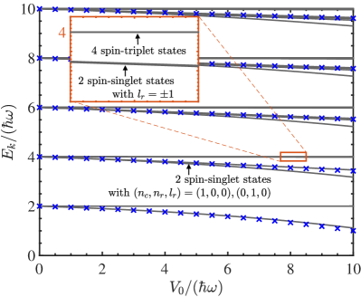
Figure 1: (Color online) The energy spectrum of two atoms $E_{k}$ in the absence of SOAM coupling as a function of the interaction strength denoted by the depth $V_{0}$ of a spherical-square-well potential, calculated by numerically solving Eq. (27) with $n=0$. The blue crosses denote the s-wave energy spectrum $E=E_{rel}^{(s)}+\hbar\omega$ consisting of the ground c.m. energy with $n_{c}=0$ and the relative energy $E_{rel}^{(s)}$ obtained by solving Eq. (37). The inset zooms in the tiny region near $V_{0}=8\hbar\omega$ and $E_{k}=4\hbar\omega$ to emphasize four spin-triplet and two spin-singlet states. Here, we have set a relatively small interaction range $\epsilon=0.3a_{\mathrm{ho}}$.

The radial equation of the relative motion in Eq. (31) can be solved analytically for an SSW potential. Let us consider the ${\it s}$-wave solution ($l_{r}=0$) as an example. The solution outside the range of the interaction, i.e., $r>\epsilon$, takes the form of (unnormalized)

$$u_{0}^{>}\left(r\right)=e^{-r^{2}/2d^{2}}U\left(-\nu,1,\frac{r^{2}}{d^{2}}\right),$$ (34)

where $d=\sqrt{\hbar/\mu\omega}=\sqrt{2}a_{\mathrm{ho}}$ is the harmonic length for the relative motion, and $\nu$ constructs the ${\it s}$-wave relative-motion energy as

$$E_{rel}^{(s)}=\left(2\nu+1\right)\hbar\omega.$$ (35)

Here, $U\left(a,b,z\right)$ is the Kummer function of the second kind, which satisfies the boundary condition at a large distance, i.e., $u_{0}^{>}\left(r\to\infty\right)\sim 0$. Inside the interaction range, the radial wave function has the form of

$$u_{0}^{<}\left(r\right)=ce^{-r^{2}/2d^{2}}M\left(-\kappa,1,\frac{r^{2}}{d^{2}}\right)$$ (36)

with $\kappa=\nu+V_{0}/2\hbar\omega$. Here, $M\left(a,b,z\right)$ is the Kummer function of the first kind, which guarantees the wave function being finite at $r=0$, i.e., $u_{0}^{<}\left(r\to 0\right)\sim\mathrm{const}\neq 0$. By using the continuity condition of the radial wave function and its first-order derivative at $r=\epsilon$, we obtain the equation satisfied by the energy $E_{rel}^{(s)}$

$$\nu\frac{U\left(1-\nu,2,\epsilon^{2}/2a_{\mathrm{ho}}^{2}\right)}{U\left(-\nu,1,\epsilon^{2}/2a_{\mathrm{ho}}^{2}\right)}+\kappa\frac{M\left(1-\kappa,2,\epsilon^{2}/2a_{\mathrm{ho}}^{2}\right)}{M\left(-\kappa,1,\epsilon^{2}/2a_{\mathrm{ho}}^{2}\right)}=0.$$ (37)

After solving Eq. (37), we could depict the total energy spectrum via $E=E_{cm}+E_{rel}^{(s)}$ for the $s$-partial wave in the absence of SOAM coupling.

In Fig. 1, we present the typical two-body energy spectrum as a function of the SSW depth $V_{0}$ in a harmonic trap. The grey curves indicate the two-body spectrum obtained by numerically solving Eq. (27) in the absence of SOAM coupling, i.e., setting $n=0$. The blue crosses denote the s-wave energy spectrum $E=E_{rel}^{(s)}+\hbar\omega$ consisting of the ground c.m. energy with $n_{c}=0$ and the relative energy $E_{rel}^{(s)}$ obtained by solving Eq. (37). As we anticipate, the degeneracies of energy levels in the spin-singlet channel are partially lifted by interaction while the spin-triplet states remain still. Taking the energy levels near $E=4\hbar\omega$ for example, there are four degenerate states in the spin-triplet channel, which are not affected by interaction. Instead, four previously degenerate states in the spin-singlet channel split into three as the SSW depth $V_{0}$ increases, two of which, corresponding to $l_{r}=\pm 1$, are still degenerate, see the inset. In the figure, one can see that these analytical energies denoted by the blue crosses are in excellent agreement with the corresponding numerical results via Eq. (27) (i.e., lines counting for the $s$-wave case).

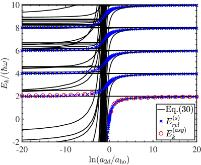
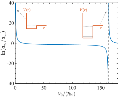
Figure 2: (Color online) (Left) The energy spectrum of two atoms $E_{k}$ in the absence of SOAM coupling as a function of the introduced 2D scattering length $\ln{(a_{2d}/a_{\mathrm{ho}})}$ via Eq. (38) for a spherical-square-well potential. The solid lines are obtained by numerically solving Eq. (27) with $n=0$, the blue crosses denote the specific total energy $E_{rel}^{(s)}+\hbar\omega$ with the s-wave relative energy $E_{rel}^{(s)}$ calculated by solving the analytic expression Eq. (37), while the red circles indicate the asymptotic behavior of the total energy $E^{(asy)}_{k}$, i.e., Eq. (39), in the non-interacting limit. (Right) The s-wave scattering length in 2D as a function of the spherical-square-well depth. The insets illustrate the position of resonance when a bound state appears near the threshold.

For ultracold atoms, the s-wave interaction is usually parameterized by the universal scattering length. Following Ref. [58], we introduce a 2D scattering length for the SSW interaction by

$$\ln\frac{a_{2d}}{a_{\mathrm{ho}}}=\frac{J_{0}\left(\sqrt{m\epsilon^{2}V_{0}/\hbar^{2}}\right)}{\sqrt{m\epsilon^{2}V_{0}/\hbar^{2}}J_{1}\left(\sqrt{m\epsilon^{2}V_{0}/\hbar^{2}}\right)}-\ln\frac{2a_{\mathrm{ho}}}{\epsilon e^{\gamma_{E}}},$$ (38)

where $\gamma_{E}$ is the Euler gamma constant, and $J_{\nu}\left(\cdot\right)$ is the Bessel function of the first kind, see the detailed derivation in Appendix B. In Fig. 2, we present the two-body energy spectrum $E_{k}$ as a function of this introduced scattering length $\ln(a_{2d}/a_{\mathrm{ho}})$. Similarly, the solid curves indicate the total energy including different partial waves obtained by numerically solving Eq. (27), while the blue crosses denote the analytically derived $s$-wave energy spectrum $E_{rel}^{(s)}+\hbar\omega$ counting the ground c.m. energy. Furthermore, the asymptotic behaviour of the $s$-wave energy spectrum $E^{(asy)}_{k}$ in non-interacting limit around $E_{k}=2(k+1)\hbar\omega$ ($k=0,1,2,\cdots$) takes an explicit form of [58]

$$E^{(asy)}_{k}\cong 2\left(k+1\right)-\frac{2}{\ln{2}+2\ln{(a_{2d}/a_{\mathrm{ho}})}}\;,$$ (39)

as denoted by red circles near the energy level $E_{k}=2\hbar\omega$ in the figure. Here, the ground-state energy of the c.m. motion is also included. In general, both the analytic results $E_{rel}^{(s)}$ and $E^{(asy)}_{k}$ show an excellent agreement with the corresponding ones in our numerical calculations. Unlike the situation in three dimensions, the two-body bound state appears even for an extremely shallow depth $V_{0}$ in 2D. This implies a positive 2D scattering length for an arbitrary SSW depth. The scattering resonance occurs, corresponding to $\ln\left(a_{2d}/a_{\text{ho}}\right)\to+\infty$ or $V_{0}\to 0$ as shown in the right plot of Fig. 2, in the non-interacting limit, once the bound state appears. Thus the energy spectrum tends to the non-interacting result of Eq. (33). The binding energy of the two-body bound state increases (but negative) as the SSW depth increases. During this process, the 2D scattering length decreases to zero, i.e., $\ln\left(a_{2d}/a_{\text{ho}}\right)\to-\infty$, before the next two-body bound state appears. The energy spectrum then tends to approach the non-interacting result again.

V.2 With SOAM coupling

We now turn to discuss the role of SOAM coupling by taking into account a nonzero $n$ (the orbital angular momentum transferred to atoms in the Raman process) and solving Eq. (27) numerically.

V.2.1 Energy spectrum

After considering the SOAM coupling by setting $n=2$, the calculated two-body energy spectrum is presented as a function of the SSW depth $V_{0}$ in Fig. 3. Under the interplay between the SOAM coupling and interaction, the degeneracy of each energy level is further lifted. This can be understood as follows. The interaction lifts the degeneracy of the energy levels in the spin-singlet channel, while the energy spectrum in the spin-triplet channel is unchanged as we have found in the absence of SOAM coupling. However, the SOAM coupling will mix the spin-singlet and spin-triplet states since the total spin is no longer conserved as expected. As a consequence, it gives rise to the additional splitting of energy levels and the elimination of energy degeneracies.

In order to further understand the underlying physics of the two-body spectrum in the presence of SOAM coupling, let us adopt a perturbation analysis of Eq. (18) in the weakly-interacting limit, i.e., $V_{0}/\hbar\omega\ll 1$. In the absence of interaction, i.e., $V_{0}=0$, the Hamiltonian $H$ is readily diagonalized in the non-interacting basis

$$\psi_{\uparrow\downarrow}\left({\bf r}_{1},{\bf r}_{2}\right) = u^{k_{1}}_{l,\uparrow}\left(r_{1}\right)u^{k_{2}}_{-l,\downarrow}\left(r_{2}\right)\frac{e^{il\phi}}{\sqrt{2\pi}}\equiv\left|k_{1},k_{2};l,\uparrow\downarrow\right\rangle,$$

$$\psi_{\downarrow\uparrow}\left({\bf r}_{1},{\bf r}_{2}\right) = u^{k_{1}}_{l,\downarrow}\left(r_{1}\right)u^{k_{2}}_{-l,\uparrow}\left(r_{2}\right)\frac{e^{il\phi}}{\sqrt{2\pi}}\equiv\left|k_{1},k_{2};l,\downarrow\uparrow\right\rangle,$$

where we note that $l_{1}=-l_{2}\equiv l$ required by the zero total angular momentum $L_{z}=l_{1}+l_{2}=0$ and $\phi\equiv\varphi_{1}-\varphi_{2}$. Then we can derive the two-body spectrum by

$$\begin{bmatrix}\psi_{\uparrow\downarrow}^{*},&\psi_{\downarrow\uparrow}^{*}\end{bmatrix}\begin{bmatrix}\hat{H}_{\uparrow\downarrow}^{(0)}&0\\ 0&\hat{H}_{\uparrow\downarrow}^{(0)}\end{bmatrix}\begin{bmatrix}\psi_{\uparrow\downarrow}\\ \psi_{\downarrow\uparrow}\end{bmatrix}=\begin{bmatrix}E_{\uparrow\downarrow}&0\\ 0&E_{\downarrow\uparrow}\end{bmatrix},$$ (40)

with

$$E_{\uparrow\downarrow} = 2\left(k_{1}+k_{2}+\left|l-n\right|+1\right)\hbar\omega,$$ (41a)

$$E_{\downarrow\uparrow} = 2\left(k_{1}+k_{2}+\left|l+n\right|+1\right)\hbar\omega.$$ (41b)

It’s straightforward to see that the energy spectrum becomes even times of the harmonic trapping energy as $E=2\hbar\omega,4\hbar\omega,6\hbar\omega,\cdots$. Let us focus the discussion on the lowest two energy levels as an example, i.e., degenerate $E_{\uparrow\downarrow}=E_{\downarrow\uparrow}=2\hbar\omega$, corresponding to the states $\left|k_{1},k_{2};l,\uparrow\downarrow\right\rangle$=$\left|0,0;n,\uparrow\downarrow\right\rangle$ and $\left|k_{1},k_{2};l,\downarrow\uparrow\right\rangle$=$\left|0,0;-n,\downarrow\uparrow\right\rangle$. Therefore, we have the lowest energy $E_{0}^{(0)}=2\hbar\omega$ with a two-fold degeneracy, manifested as

$$H^{(0)}\left|\Psi_{1}^{(0)}\right\rangle = E_{0}^{(0)}\left|\Psi_{1}^{(0)}\right\rangle,$$ (42a)

$$H^{(0)}\left|\Psi_{2}^{(0)}\right\rangle = E_{0}^{(0)}\left|\Psi_{2}^{(0)}\right\rangle,$$ (42b)

with the unperturbed Hamiltonian

$$H^{(0)}\equiv\begin{bmatrix}\hat{H}_{\uparrow\downarrow}^{(0)}&0\\ 0&\hat{H}_{\uparrow\downarrow}^{(0)}\end{bmatrix},$$ (43)

and two associated degenerate states

$$\left|\Psi_{1}^{(0)}\right\rangle\equiv\begin{bmatrix}\left|0,0;n\right\rangle\\ 0\end{bmatrix},~{}\left|\Psi_{2}^{(0)}\right\rangle\equiv\begin{bmatrix}0\\ \left|0,0;-n\right\rangle\end{bmatrix}.$$ (44)

When the interaction $V$ is turned on, but small, we may utilize the degenerate perturbation theory to see how this two-fold degeneracy of the lowest energy is lifted. The unperturbed wave function $\left|\Psi^{(0)}\right\rangle$ can be expanded as a linear combination of $\left\{\left|\Psi_{1}^{(0)}\right\rangle,\left|\Psi_{2}^{(0)}\right\rangle\right\}$ in the degenerate sub-Hilbert space, i.e.,

$$\left|\Psi^{(0)}\right\rangle=\alpha_{1}\left|\Psi_{1}^{(0)}\right\rangle+\alpha_{2}\left|\Psi_{2}^{(0)}\right\rangle.$$ (45)

The perturbed Hamiltonian takes the form of

$$H=H^{(0)}+H^{(1)},$$ (46)

with the perturbation

$$H^{(1)}=\left[\begin{array}[]{cc}+V/2&-V/2\\ -V/2&+V/2\end{array}\right].$$ (47)

Up to the first-order approximation, the perturbed wave function and the corresponding energy can be written as

$$\left|\Psi\right\rangle \approx \left|\Psi^{(0)}\right\rangle+\left|\Psi^{(1)}\right\rangle,$$ (48a)

$$E_{0} \approx E_{0}^{(0)}+E_{0}^{(1)},$$ (48b)

where $\left|\Psi^{(1)}\right\rangle$ and $E_{0}^{(1)}$ are the first-order corrections to the wave function and energy, respectively. After substituting the perturbed wave function and the corresponding energy back into the Schrödinger equation $H\left|\Psi\right\rangle=E_{0}\left|\Psi\right\rangle$, we get

$$H^{(0)}\left|\Psi^{(1)}\right\rangle+H^{(1)}\left|\Psi^{(0)}\right\rangle\approx E_{0}^{(0)}\left|\Psi^{(1)}\right\rangle+E_{0}^{(1)}\left|\Psi^{(0)}\right\rangle,$$ (49)

up to the first-order approximation. After taking the inner product respectively with $\left\langle\Psi_{1}^{(0)}\right|$ and $\left\langle\Psi_{2}^{(0)}\right|$, we obtain eventually the secular equation

$$\begin{bmatrix}W_{11}&W_{12}\\ W_{21}&W_{22}\end{bmatrix}\begin{bmatrix}\alpha_{1}\\ \alpha_{2}\end{bmatrix}=E_{0}^{(1)}\begin{bmatrix}\alpha_{1}\\ \alpha_{2}\end{bmatrix},$$ (50)

with the matrix element being

$$W_{mn}\equiv\left\langle\Psi_{m}^{(0)}\right|H^{(1)}\left|\Psi_{n}^{(0)}\right\rangle.$$ (51)

$\left|\Psi_{1,2}^{(0)}\right\rangle$ are just the single-body wave functions described in the previous section and thus one can straightforwardly construct the matrix of $W$. Therefore, the first-order energy correction $E_{0}^{(1)}$ can be conveniently obtained by numerically solving this secular equation. In Fig. 3 and the inset, the corrected energy $E_{0}\approx E_{0}^{(0)}+E_{0}^{(1)}$ of the $E_{0}^{(0)}=2\hbar\omega$ level is denoted by blue dots in the weak-interaction limit. We can find that the lowest two energy levels split as interaction strengthens and coincides with the exact numerical results shown in grey lines at small values of $V_{0}$.

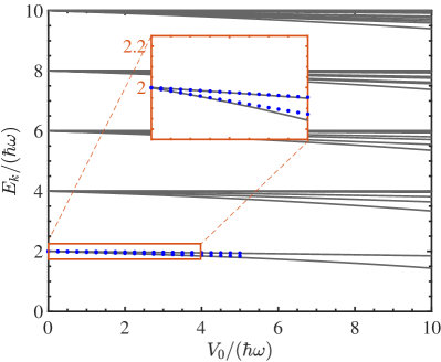
Figure 3: (Color online) The energy spectrum of two atoms $E_{k}$ in the presence of SOAM coupling as a function of the spherical-square-well depth $V_{0}$, calculated by numerically solving Eq. (27) with $n=2$. The blue dots indicate the lowest two energy levels at small $V_{0}$, calculated from the perturbation approach. The inset zooms in the tiny region near $E_{k}=2\hbar\omega$ with $V_{0}/\hbar\omega$ varying from 0 to 4.

By taking a relatively small interaction strength $V_{0}=2\hbar\omega$, we further illustrate these two lowest energy levels as functions of the transferred orbital angular momentum $n$ in Fig. 4. The numerically calculated energies in blue dots show a great agreement with the one from the perturbation approach denoted by red circles. Surprisingly, we find that the separate energy levels due to interactions tend to approach each other and restore approximately the degeneracy as $n$ increases. This can be explained by the perturbation theory as follows. To the first-order approximation, we find that the off-diagonal elements $W_{12}=W_{21}$ of the matrix $W$ in Eq. (50) decrease towards zero as $n$ increases, while the diagonal elements $W_{11}=W_{22}$ are irrelevant to $n$. Therefore, the off-diagonal elements are becoming negligible compared to the diagonal elements at large $n$, leading to no level repulsion and a tendency of degeneracy. The weak interaction introduces only a uniform shift to previously splitting energy levels.

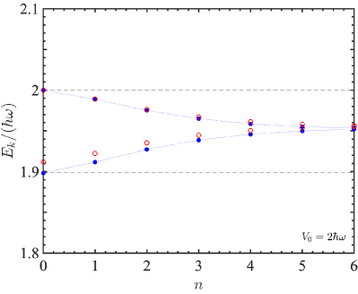
Figure 4: (Color online) Lowest two energy levels $E_{k}$ of two atoms in a harmonic trap with the SOAM coupling, as a function of the transferred orbital angular momentum $n$ at a small spherical-square-well depth $V_{0}=2\hbar\omega$. The numerical results in blue dots are compared with the one calculated from the perturbation approach denoted by red circles.

V.2.2 Correlations

We turn to discuss the correlations of two atoms by introducing a correlation function or an integrated density function. If we fix the position of the atom $1$, for example, at ${\bf r}_{1}$, the probability of finding the atom $2$ at the position ${\bf r}_{2}$ is $\left|\Psi\left({\bf r}_{1},{\bf r}_{2}\right)\right|^{2}$. Therefore, the total probability of the atom $2$ appearing at the position ${\bf r}_{2}$ is simply obtained by integrating over all ${\bf r}_{1}$, and that is

$$g\left({\bf{r}}_{2}\right)=\int d{\bf r}_{1}\left|\Psi\left({\bf r}_{1},{\bf r}_{2}\right)\right|^{2}.$$ (52)

The function $g\left({\bf{r}}_{2}\right)$ characterizes the intrinsic correlation between the two atoms. In Fig. 5, the correlation function $g\left(r_{2}\right)$ is plotted as a function of $r_{2}=\left|{\bf{r}}_{2}\right|$ and the SSW depth $V_{0}$ for the two lowest-energy states around $E=2\hbar\omega$. Here, we have also integrated out the angular part with respect to $\varphi_{2}$.

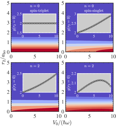
Figure 5: (Color online) Contour plots of correlation functions $g\left(r_{2}\right)$ of two lowest states for energy level $E_{k}=2\hbar\omega$, i.e., second-lowest and lowest energy levels respectively in Fig. 1 and Fig. 3, as functions of radius $r_{2}$ and the spherical-square-well depth $V_{0}$. In the insets, the specific values of correlation functions at $r_{2}=0$ are depicted as a function of $V_{0}$.

In the absence of SOAM coupling, i.e., $n=0$ shown by the upper panel in Fig. 5, the system in the non-interacting limit is nothing but two free atoms. The two-body wave function is simply the product of two single-particle ground-state wave functions, i.e., $e^{-r^{2}_{1,2}/2a_{\mathrm{ho}}^{2}}/\sqrt{\pi}a_{\mathrm{ho}}$. After some straightforward algebra, we derive $g\left(r_{2}\right)=2e^{-r_{2}^{2}/a_{\mathrm{ho}}^{2}}$ which yields $g\left(r_{2}\right)=2$ at $r_{2}=0$. The correlation in the spin-singlet channel increases as the interaction strength increases, while it remains unchanged in the spin-triplet channel as anticipated since the interaction appears only in the spin-singlet channel, i.e., Eq. (4). In sharp contrast, when the SOAM-coupling effect is included, e.g., $n=2$ shown by the lower panel in Fig. 5, the states in the spin-singlet and spin-triplet channels are closely coupled. We find that the SOAM coupling plays a crucial role and both correlation functions at $r_{2}=0$ of these two lowest-energy states exhibit a strong dependence on the interaction strength.

VI Conclusions

We have studied the roles of spin-orbital-angular-momentum coupling and a two-body interaction potential in the underlying physics of two harmonically trapped atoms by addressing the associated two-body energy spectrum and correlations. Starting from the two-body Hamiltonian counting a tunable interaction potential and the spin-orbital-angular-momentum coupling, we have derived an explicit secular equation for numerically calculating the associated eigenenergy and eigenfunction. In the absence of spin-orbital-angular-momentum coupling, the calculated energy spectrum can well reproduce the analytic result in previous works, i.e., only the spin-singlet states are significantly affected by the two-body interaction and the degeneracies in the energy spectrum disappear gradually as the interaction strength rises.

In the presence of spin-orbital-angular-momentum coupling, we have made a careful analysis of the two-body spectrum and the correlation as functions of the interaction strength as well as the transferred orbital angular momentum. We first develop a perturbation approach to justify the numerical result in the weak-interaction limit, which demonstrates the crucial role of the interplay between the interaction and spin-orbital-angular-momentum coupling in the elimination of energy-level degeneracy as the interaction enhances. In addition, we have introduced a correlation function, i.e., an integrated one-body density function, to characterize the behavior of two-body wave functions with respect to the interaction strength as well as the radius with and without spin-orbital-angular-momentum coupling. The correlations show direct evidence of the mixing of the spin-triplet and spin-singlet wave functions due to spin-orbital-angular-momentum coupling. At large transferred angular momentum, we find that the deviated energy levels of the lowest two states due to a definite weak interaction tend to approach each other and restore the degeneracy as the strength of spin-orbital-angular-momentum coupling increases. This intriguing behavior is further explained by employing the perturbation approach.

We have focused our study in the subspace of two definite conserved quantum numbers, corresponding to vanishing total orbital angular momentum $L_{z}$ and total spin $S_{z}$ along the $z$ axis. This could be conveniently generalized to non-zero values of $L_{z}$ and $S_{z}$. In addition, the transverse effective Zeeman field has been neglected here due to the weak light-atom coupling in space in the present experimental setup, which may also be further considered according to the exact diagonalization method.

Appendix A Decomposing of $V\left(r_{12}\right)$ in the angular basis

Let us expand the interaction potential $V\left(r_{12}\right)$ in the basis of the angular eigenstates of $\hat{l}_{1z}$ and $\hat{l}_{2z}$. To this end, the two-body potential can be written as

$$V\left(r_{12}\right)=\int d{\bf r}V\left(r\right)\delta\left({\bf r}_{1}-{\bf r}_{2}-{\bf r}\right).$$ (53)

Since we have

$$\delta\left({\bf r}\right)=\frac{1}{\left(2\pi\right)^{2}}\int d{\bf k}e^{i{\bf k}\cdot{\bf r}},$$ (54)

it yields

$$V\left(r_{12}\right)=\int d{\bf r}\frac{V\left(r\right)}{\left(2\pi\right)^{2}}\int d{\bf k}e^{i{\bf k}\cdot\left({\bf r}_{1}-{\bf r}_{2}-{\bf r}\right)}.$$ (55)

By using the two-dimensional plane wave expansion,

$$e^{i{\bf k}\cdot{\bf r}}=\sum_{l=-\infty}^{\infty}i^{l}J_{l}\left(kr\right)e^{il\left(\varphi_{{\bf k}}-\varphi_{{\bf r}}\right)},$$ (56)

we find

$$V\left(r_{12}\right) = \int d{\bf r}\frac{V\left(r\right)}{\left(2\pi\right)^{2}}\int d{\bf k}e^{i{\bf k}\cdot\left({\bf r}_{1}-{\bf r}_{2}\right)}\cdot e^{-i{\bf k}\cdot{\bf r}}$$ (57)

$$= \frac{1}{2\pi}\int_{0}^{\infty}V\left(r\right)rdr\int e^{i{\bf k}\cdot\left({\bf r}_{1}-{\bf r}_{2}\right)}J_{0}\left(kr\right)kdkd\varphi_{{\bf k}}$$

$$= \sum_{l=-\infty}^{\infty}V_{l}\left(r_{1},r_{2}\right)e^{-il\left(\varphi_{1}-\varphi_{2}\right)}$$

with

$$V_{l}\left(r_{1},r_{2}\right)=\int_{0}^{\infty}rdrV\left(r\right)\int_{0}^{\infty}kdkJ_{0}\left(kr\right)J_{l}\left(kr_{1}\right)J_{l}\left(kr_{2}\right).$$ (58)

Appendix B Scattering parameters for a spherical-square-well potential

Let us consider the scattering problem of two atoms interacting with a spherical-square-well potential in 2D. The relative motion of two atoms is described by the following equation

$$\left[-\frac{\hbar^{2}}{m}\nabla^{2}+V\left({\bf r}\right)\right]\psi\left({\bf r}\right)=E\psi\left({\bf r}\right)$$ (59)

with

$$V\left({\bf r}\right)=\begin{cases}-V_{0},&0\leq r\leq\epsilon,\\ 0,&r>\epsilon,\end{cases}$$ (60)

and $E>0$ for a scattering problem. The angular momentum is a good quantum number, thus the wave function is written as $\psi\left({\bf r}\right)=u_{l}\left(r\right)e^{il\varphi}/\sqrt{2\pi},$which yields the radial equation

$$\left[\frac{1}{r}\frac{\partial}{\partial r}r\frac{\partial}{\partial r}-\frac{l^{2}}{r^{2}}+k^{2}-\frac{mV\left(r\right)}{\hbar^{2}}\right]u_{l}\left(r\right)=0$$ (61)

with $k^{2}=mE/\hbar^{2}$. For the $s$-wave scattering, i.e., $l=0$, the solution takes the form of By solving the equation, we conveniently obtain

$$u_{0}\left(r\right)=\begin{cases}cJ_{0}\left(Gr\right),&0\leq r\leq\epsilon,\\ \cot\delta_{0}\cdot J_{0}\left(kr\right)-N_{0}\left(kr\right),&r>\epsilon,\end{cases}$$ (62)

where $\delta_{0}$ is the $s$-wave scattering phase shift, $c$ is a normalization parameter, and $G^{2}=k^{2}+mV_{0}/\hbar^{2}$. Here, $J_{\nu}\left(\cdot\right)$ and $N_{\nu}\left(\cdot\right)$ are Bessel functions of the first and second kinds. By using the continuity condition of the wave function and its first-order derivative at $r=\epsilon$, we easily obtain the scattering phase shift

$$\cot\delta_{0}=\frac{\left(k\epsilon\right)J_{0}\left(G\epsilon\right)N_{1}\left(k\epsilon\right)-\left(G\epsilon\right)J_{1}\left(G\epsilon\right)N_{0}\left(k\epsilon\right)}{\left(k\epsilon\right)J_{0}\left(G\epsilon\right)J_{1}\left(k\epsilon\right)-\left(G\epsilon\right)J_{1}\left(G\epsilon\right)J_{0}\left(k\epsilon\right)}.$$ (63)

Expanding $\cot\delta_{0}$ at small $k$, we obtain the effective-range expansion of the scattering phase shift in 2D, i.e.,

$$\cot\delta_{0}=\frac{2}{\pi}\ln\left(ka_{2D}\right)+O\left(k^{2}\right)$$ (64)

with the 2D $s$-wave scattering length

$$\ln\frac{a_{2D}}{\epsilon}=\frac{J_{0}\left(\sqrt{\tilde{V}_{0}}\right)}{\sqrt{\tilde{V}_{0}}J_{1}\left(\sqrt{\tilde{V}_{0}}\right)}+\gamma_{E}-\ln 2,$$ (65)

with Euler gamma constant $\gamma_{E}\approx 0.577216$ and $\tilde{V}_{0}\equiv V_{0}/\left(\hbar^{2}/m\epsilon^{2}\right)$, or in a form of

$$\ln\frac{a_{2d}}{a_{\mathrm{ho}}}=\frac{J_{0}\left(\sqrt{m\epsilon^{2}V_{0}/\hbar^{2}}\right)}{\sqrt{m\epsilon^{2}V_{0}/\hbar^{2}}J_{1}\left(\sqrt{m\epsilon^{2}V_{0}/\hbar^{2}}\right)}-\ln\frac{2a_{\mathrm{ho}}}{\epsilon e^{\gamma_{E}}}.$$ (66)

Explicitly, the relationship between this introduced scatter length $\ln{(a_{2d}/a_{\mathrm{ho}})}$ and the two-body interaction strength $V_{0}$ can be seen in the right plot of Fig. 2.