Sign problem in tensor network contraction

Abstract

We investigate how the computational difficulty of contracting tensor networks depends on the sign structure of the tensor entries. Using results from computational complexity, we observe that the approximate contraction of tensor networks with only positive entries has lower computational complexity as compared to tensor networks with general real or complex entries. This raises the question how this transition in computational complexity manifests itself in the hardness of different tensor network contraction schemes. We pursue this question by studying random tensor networks with varying bias towards positive entries. First, we consider contraction via Monte Carlo sampling, and find that the transition from hard to easy occurs when the tensor entries become predominantly positive; this can be understood as a tensor network manifestation of the well-known negative sign problem in Quantum Monte Carlo. Second, we analyze the commonly used contraction based on boundary tensor networks. The performance of this scheme is governed by the amount of correlations in contiguous parts of the tensor network (which by analogy can be thought of as entanglement). Remarkably, we find that the transition from hard to easy—that is, from a volume law to a boundary law scaling of entanglement—occurs already for a slight bias of the tensor entries towards a positive mean, scaling inversely with the bond dimension $D$, and thus the problem becomes easy the earlier the larger $D$ is. This is in contrast both to expectations and to the behavior found in Monte Carlo contraction, where the hardness at fixed bias increases with bond dimension. To provide insight into this early breakdown of computational hardness and the accompanying entanglement transition, we construct an effective classical statistical mechanical model which predicts a transition at a bias of the tensor entries of $1/D$, confirming our observations. We conclude by investigating the computational difficulty of computing expectation values of tensor network wavefunctions (Projected Entangled Pair States, PEPS) and find that in this setting, the complexity of entanglement-based contraction always remains low. We explain this by providing a local transformation which maps PEPS expectation values to a positive-valued tensor network. This not only provides insight into the origin of the observed boundary law entanglement scaling, but also suggests new approaches towards PEPS contraction based on positive decompositions.

I Introduction

I.1 Motivation

Simulating quantum many-body systems is one of the central challenges in modern physics. Its hardness stems from the exponential size of the underlying Hilbert space and the presence of intricate quantum correlations, which makes it necessary to rely on suitable approximate methods. Arguably, the most successful method for a large class of equilibrium problems is Quantum Monte Carlo (QMC) [1]. Yet, especially in systems with strong quantum correlations, QMC can be plagued by the negative sign problem, or “sign problem” for short. It originates in negative transition matrix elements in the imaginary time evolution operator $e^{-\epsilon h}$, corresponding to positive off-diagonal entries in the Hamiltonian terms $h$.

Extensive efforts have gone into finding ways to circumvent or remedy the sign problem. While in some cases, it can be overcome by a suitable basis transform, as well as modified QMC algorithms, these approaches are not successful in the general case [1]. A way out promises the use of other simulation methods which do not suffer from a sign problem, such as variational methods. In particular, tensor network methods have proven instrumental in addressing a range of strongly correlated quantum many-body problems in recent years [2]. For instance, unlike QMC, tensor network algorithms exhibit no dependence on local basis choices by construction. This raises the question whether methods such as tensor networks can indeed provide a way to circumvent to the sign problem altogether.

In order to address this question, it is first important to understand what precisely is the difficulty behind the sign problem. Importantly, the presence or absence of a negative sign problem is not directly equivalent to computational hardness of the problem, and in particular not to NP-hardness. Indeed, classical spin glasses, which do not suffer from the sign problem, are well-known to be NP-hard [3]. In those systems, the hardness of Monte Carlo algorithms stems from a sampling problem instead, that is, the hardness of setting up a Markov chain which efficiently samples from the correct probability distribution. Thus, when discussing how to remedy the sign problem, it is essential to separate these two sources of hardness, which is challenging since in certain scenarios, the NP-hardness of a classical problem (i.e., a sampling problem) can be disguised as a sign problem [4]. It is thus central that we are able to single out the intrinsic computational complexity of the sign problem.

To this end, we can use insights gained from computational complexity. In particular, the path sum encountered in QMC is an exponentially big sum, where each term (the transition amplitude) is efficiently computable. Computing such a sum is a defining problem for the class #P (“Sharp P”), which amounts to counting the number of solutions to an NP problem. In the case that the sum only contains positive terms—that is, in the absence of a negative sign problem—a famous result due to Stockmeyer [5] (“approximate counting”) states that this number can be approximated in $\textsf{BPP}^{\textsf{NP}}$, that is, by a randomized algorithm with access to a black-box which can solve NP problems. In essence, this takes the complexity of sign-problem free Hamiltonians back from #P to the much easier class NP, where also classical spin glasses lie. On the other hand, general quantum Hamiltonians are complete problems for the complexity class QMA (the quantum version of NP), which is widely believed to be much harder [6, 7, 8]. This gap in the computational complexity of general and sign-problem free Hamiltonians—assuming we believe it exists—will not simply go away by changing the method used to solve the quantum many-body problem at hand.

This raises the question as to what happens to the sign problem in tensor networks—that is, how is the different computational complexity of Hamiltonians with and without a sign problem reflected in tensor networks? The answer to this question will depend on how precisely the quantum many-body problem is mapped to tensor networks. A first possibility is to rewrite the path sum in QMC as a tensor network in one dimension higher. Then, the sign problem will exactly correspond to a tensor network which contains non-positive entries; moreover, it is conceivable that this different sign pattern will persist when compressing the tensor network in the imaginary time direction, i.e., truncating the bond dimension, such as done in simple or full update tensor network algorithms [9, 10].

This leads to the question whether there is a transition in difficulty in evaluating tensor networks with positive vs. general real or complex entries. This is precisely the question which we investigate in this work; for a description of the setup, see Fig. 1.

A first insight on the difference in the hardness of contracting tensor networks with positive entries vs. those with arbitrary entries can be obtained from looking at tensor network contraction as an exponentially big sum, where each term can be computed efficiently: In that case, Stockmeyer’s results on approximate counting tells us immediately that approximating the value of a positive tensor network is considerably easier (namely, $\textsf{BPP}^{\textsf{NP}}$). This perspective also makes it clear that the structure underlying the sign problem in QMC and in tensor network contraction is precisely the same: Both are exponentially large sums where each term individually can be efficiently computed, and the hardness of the task is governed precisely by whether the sum is over positive terms or not—the negative sign problem.

However, sampling is not how tensor networks are contracted in practice: Rather, one proceeds by contracting the tensor network piece by piece (e.g., column by column), where at each step, the contracted region is approximated by a tensor network with lower complexity [11, 12]. In order to have an efficient approximation, it is thus necessary to have a low amount of correlations in the corresponding cuts. The question thus arises whether this way of contraction is as well subject to a hardness transition when changing between positive and general entries in the tensor network. Indeed, such a transition was recently observed by Gray and Chan when benchmarking highly optimized tensor contraction routines [12]. Taken together, the above points strongly motivate a systematic study of a potential hardness transition in tensor networks as a function of their sign pattern.

I.2 Results

In this paper, we comprehensively study how the difficulty of evaluating tensor networks depends on the sign pattern of their entries: Is there a difference in the hardness of contracting tensor networks with only positive entries as compared to tensor networks with general real or complex entries? How does this depend on the contraction method chosen? And what determines the transition between the different regimes? To address these questions, we study the average-case difficulty of contracting random tensor networks, that is, tensor networks with random entries, on a regular square lattice, and with bond dimension $D$, see Fig. 1a. Here, the entries of each tensor are chosen independently Haar-random (either real or complex), with standard deviation $1$, and subsequently shifted into the positive by some amount $\lambda$ (Fig. 1b), allowing us to smoothly vary from tensor networks with completely random entries (i.e., with mean zero) to the regime of positive entries.

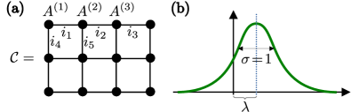
Figure 1: (a) A tensor network is constructed from local tensors $A^{(s)}$. Each leg $i_{k}$ of the tensor corresponds to an index with bond dimension $D$, $i_{k}=1,\dots,D$. Connected legs are identified and summed over (“contracted”); after contracting all legs, we obtain the value $\mathcal{C}$ of the tensor network, which is a number. We are interested in approximating $\mathcal{C}$ up to a given multiplicative error. (b) We consider random tensor networks, where each tensor is chosen Haar-random with standard deviation $\sigma=1$ (either real or complex), and displaced by a shift $\lambda$; as $\lambda$ is increased, this gradually transitions to a tensor network with predominantely positive entries around $\lambda\approx 1$.

First, we consider the contraction of the tensor network using Monte Carlo sampling, that is, by sampling the exponentially big sum described by the tensor network, and study when the function which we sum exhibits a sign problem; the hardness captured by this setup has the same structure as the sign problem in other Monte Carlo schemes, in particular QMC. We observe a transition around $\lambda\approx 1$, that is, when the entries of the network become predominantly positive; this is in line with the complexity theoretic reasoning we gave above (right before Section I.2) based on approximate counting. In addition, we find that for unbiased (or slightly biased) random tensors with $\lambda\lesssim 1/D$, the hardness of the problem saturates at the worst-case scaling $D^{N}$, while for larger bias $\lambda$, the severity of the sign problem decays as a function of $\lambda$ in a way that is independent of the bond dimension.

We then move on to the hardness of the commonly used entanglement-based contraction—that is, where the contracted region is approximated by a low-entanglement state, and the hardness depends on the amount of correlations (entanglement) in the tensor network. We observe that the problem again exhibits a transition from hard to easy, and thus an entanglement transition from a high-entanglement (volume law) to a low-entanglement (boundary law) regime. In studying this transition, we however find something extraordinarily surprising: The transition from hard to easy occurs for an ever smaller bias $\lambda$ towards a positive distribution as the bond dimension $D$ is increased. Specifically, for bond dimension $D$, a shift $\lambda\approx 1/D$ already induces a transition to a low-entanglement regime, even though this amounts to a disbalance in the sign pattern of the order of only $1/D$. We establish the existence of this transition both through the study of random instances, as well as through the mapping to an effective statistical mechanics model, which becomes accurate in the large-$D$ limit and exhibits a transition at $\mu\coloneqq\lambda D=1$ for large $D$. Subsequently, we demonstrate that this transition indeed has its origin in the shift towards positive entries, and not in the simultaneously induced decoupling of the network into local tensor products: To this end, we study the two causes separately, and find that they lead to vastly different effects, regarding both the point and the sharpness of the transition.

As a last point, we return to the use of tensor networks with open physical indices, in particular Projected Entangled Pair States (PEPS), as a variational ansatz $\lvert\psi\rangle$ for quantum many-body wavefunctions. The central primitive needed to accurately evaluate quantities in a PEPS $\lvert\psi\rangle$ is the computation of the normalization $\langle\psi\lvert\psi\rangle$. We analyze the difficulty of this problem for random PEPS tensors with complex entries, and find that both random instances and the mapping to a statmech model in the large-$D$ limit (for the latter, see also Ref. [13]) predict that the problem of computing $\langle\psi\lvert\psi\rangle$ is easy, that is, the underlying tensor network (without any physical indices) exhibits a boundary-law entanglement scaling. We then give a complexity theoretic underpinning of this result, by showing that the “completely positive” double-layer structure of the problem can be used to rewrite the contraction as a sum of efficiently computable positive terms for sufficiently large $D$. This in turn implies that the PEPS contraction can be approximated much more efficiently than a general sum, using Stockmeyer’s approximate counting (thus taking it from #P to $\textsf{BPP}^{\textsf{NP}}$), as well as through sign-problem free Monte Carlo sampling. In addition, this provides an alternative explanation for the boundary-law entanglement scaling, by showing that PEPS expectation values are effectively just positive tensor networks, modulo a local transformation.

II Setup

Let us start by defining tensor networks, cf. Fig. 2. A tensor network, w.l.o.g. on a two-dimensional square lattice, is given by a set of four-index tensors $\{A^{(s)}_{x_{\ell}x_{r}x_{u}x_{d}}\}_{s}$, where $A^{(s)}$ corresponds to site $s=1,\dots,N$, the indices $x_{\bullet}=1,\dots,D$ (with $D$ called the bond dimension) are associated to edges, and indices of adjacent tensors which are associated to the same edge $e$ have the same value $x_{e}$. Let

$$T(\bm{x})\coloneqq\prod_{s}A^{(s)}_{\bm{x}}\ ,$$ (1)

where $\bm{x}=(x_{e})_{e}$ contains the value of $x_{e}$ for all edges in the network, and each $A^{(s)}_{\bm{x}}$ only depends on the $x_{e}$ of the adjacent edges—that is, $T(\bm{x})$ is the value taken by the tensor network if each edge is assigned the value $x_{e}$. The value (or contraction) of the tensor network is then given by

$$\mathcal{C}\equiv\mathcal{C}(\{A^{(s)}\})\coloneqq\sum_{\bm{x}}T(\bm{x})\ ,$$ (2)

where the sum runs over all $D^{N}$ values of $\bm{x}$. Note that this construction can be easily adapted to different boundary conditions, by choosing fewer-index tensors at the boundary when necessary, and similarly to other graphs.

Figure 2: (a) A tensor network (here on a 2D square lattice) is constructed by placing tensors $A^{(s)}_{x_{\ell}x_{r}x_{u}x_{d}}$ at site $s$. The indices $x_{\bullet}=1,\dots,D$ are associated to the left, right, up, and down edge adjacent to site $s$, respectively; e.g., the central tensor in panel (a) is $A^{(5)}_{x_{6}x_{7}x_{9}x_{4}}$. For a given configuration $\bm{x}=(x_{1},x_{2},\dots)$ of edges, $T(\bm{x})$ denotes the value of the product of all tensors for the given values of $\bm{x}$. (b) The value of the tensor network $\mathcal{C}\equiv\mathcal{C}(\{A^{(s)}\})$ is then obtained by contracting the tensor network, i.e., by summing $T(\bm{x})$ over all values $\bm{x}$ of the indices.

Tensor networks naturally appear as discretized partition functions $\mathrm{tr}(e^{-\beta H})$, where the $x_{e}$ are either configurations at a given point $e$ in space and (imaginary) time; or as collapsed partition functions, where an edge $e$ corresponds to a point in space, and $x_{e}$ holds the configuration at all time slices simultaneously. For sign problem free Hamiltonians, this naturally leads to tensor networks with only positive entries (“positive tensor networks”), while general Hamiltonians will generally carry negative or complex entries (“non-positive tensor networks”). This raises the question whether there is a transition in the difficulty of evaluating Eq. (2) when transitioning from positive to non-positive tensor networks. Indeed, such a transition has recently been observed by Gray and Chan in benchmarking tensor contraction codes [12].

Before analyzing the reason for this transition, let us specify the setting we consider. While part of our arguments apply to general tensor networks, some of them require tensor networks where the tensors $\{A^{(s)}\}$ are suitably chosen at random. Whenever we discuss concrete instances, we will draw each tensor from a displaced Haar-random real or complex distribution, i.e.,

$$A^{(s)}_{x_{\ell}x_{r}x_{u}x_{d}}=D^{2}U^{(s)}_{(x_{\ell}x_{r}x_{u}x_{d})}+\lambda\ ,$$ (3)

where $U$ is a Haar-random real or complex vector (i.e., the first column of a Haar-random orthogonal or unitary matrix $\mathcal{U}$), respectively. Here, the normalization is chosen such that the entries of $D^{2}U$ have a typical magnitude of $1$ (indeed, subblocks of $D^{2}\mathcal{U}$ converge to a random real or complex Gaussian ensemble with standard deviation $1$ and mean $0$). Adding $\lambda\geq 0$ displaces the distribution, such that the entries of $A^{(s)}$ become mostly positive (or centered around the positive axis for complex $U$) for $\lambda\gtrsim 1$.

In the entire discussion, we will always be interested in the difficulty of approximating $\mathcal{C}(\{A^{(s)}\})$ up to multiplicative accuracy. This is the natural scenario in particular when we need to take ratios of tensor network contractions, where good relative accuracies are required for the denominator; this setting is natural both in tensor network simulations and in contexts where sign problems are relevant in QMC simulations.

III Monte Carlo based contraction

Let us first show that non-positive tensor networks do indeed exhibit a Monte Carlo sign problem which is not present in positive tensor networks. To this end, note that Eq. (2) is an exponentially big sum, over a discrete configuration space $\bm{x}$, of a function $T(\bm{x})$ which can be efficiently evaluated for fixed $\bm{x}$. Thus, we can use Monte Carlo sampling over $\bm{x}$ to approximate $\mathcal{C}$. The multiplicative error which we obtain for the approximation will depend on the sign pattern of $T(\bm{x})$: If all $T(\bm{x})$ point in the same direction in the complex plane, which does happen around $\lambda\gtrsim 1$, there are no cancellations and we expect rapid convergence. On the other hand, for small $\lambda$, where $A^{(s)}_{\bm{x}}$ and thus $T(\bm{x})$ is distributed around the origin, we expect strong cancellations, and thus a slow convergence of the relative accuracy of the sample.

The severity of such a Monte Carlo sign problem can be quantified by comparing the values of the “fermionic partition function” $\mathcal{C}$, Eq. (2), with the “bosonic” one, $\mathcal{C}_{b}=\sum_{\bm{x}}|T(\bm{x})|$, where we take the absolute value of $T(\bm{x})$ [4, 15]. One expects both quantities to scale exponentially with the volume (i.e., the number of lattice sites) $N$, and thus their ratio should scale with a “free energy density difference” $\Delta f$, defined through

$$e^{-\Delta f\,N}\coloneqq\frac{\mathcal{C}}{\mathcal{C}_{b}}=\frac{\sum_{\bm{x}}T(\bm{x})}{\sum_{\bm{x}}|T(\bm{x})|}$$ (4)

for $N\to\infty$. Since we expect the mean of $K$ samples of $|T(\bm{x})|$ to converge as $1/\sqrt{K}$—but not better, in particular not exponentially fast either in $K$ or in the system size $N$—and the same scaling of fluctuations will show up when sampling $T(\bm{x})$, a $\Delta f>0$ implies that an exponential number of sample points $K\sim\exp(2\,\Delta f\,N)$ will be required to get a good approximation, and thus signals the presence of a sign problem (which becomes relevant as soon as $N\gtrsim 1/\Delta f$).

Fig. LABEL:fig:free-energy shows the average $\Delta f$ as a function of $\lambda$ for different bond dimensions $D$, both for Haar-random orthogonal and unitary tensors. We can identify three different regimes: First, for $\lambda\leq\eta_{0}/D$ (with $\eta_{0}\approx 1$), $\Delta f$ is constant, with a value $\Delta f=\log D+\mathrm{const.}$, as can be seen from the data collapse for all $D$ except $D=2$ in Fig. LABEL:fig:free-energyb (with the constant depending on the choice of the random ensemble). Thus, $e^{\Delta f}\sim D^{N}$, which is consistent with the expected worst-case $D^{N}$ scaling (corresponding to exact contraction). However, once outside this regime, the $\Delta f(\lambda)$ for different $D$ collapse more or less perfectly, with only minor deviations for $D=2$. $\Delta f(\lambda)$ then exhibits two different regimes: For $\eta_{0}/D\leq\lambda\lesssim 1$, we see a behavior $\Delta f\sim-\log\lambda$ (as expected from the collapse in Fig. LABEL:fig:free-energyb and the transition at constant $\lambda D$). For $\lambda\gg 1$, the scaling behavior depends on the chosen distribution—for Haar-orthogonal tensors, $\Delta f$ decays super-exponentially, while for Haar-unitary tensors, $\Delta f\sim\lambda^{2}/4$ (Fig. LABEL:fig:free-energyd,e). The latter behavior can be understood from the fact that for Haar-orthogonal tensors, only a Gaussian tail contributes to negative amplitudes, while for Haar-unitary tensors which are shifted by $\lambda\gg 1$ into the positive, the phase of the tensor still fluctuates by $\sim 1/\sqrt{\lambda}$ around zero. For comparison, we have also considered tensor networks with real or complex Gaussian entries (shown in Fig. LABEL:fig:free-energy with semi-transparent markers), which show the same behavior to very high accuracy; one difference, however, is the behavior for large $\lambda$ in the real case, as for Haar-orthogonal tensors, $\Delta f\equiv 0$ as soon as $\lambda\geq D^{2}$, and thus, the decay for large $\lambda$ must be more rapid (as can be seen in Fig. LABEL:fig:free-energyd for the $D=2$ data).

From Fig. LABEL:fig:free-energy, we conclude that on the one hand, for very small $\lambda$, the severity of the sign problem depends on the bond dimension of the tensor network, and increases with larger $D$. For $1/D\lesssim\lambda\lesssim 1$, this transitions into a regime where there is still a sign problem, which however is independent of the bond dimension. Only for $\lambda\gtrsim 1$, the sign problem starts to disappear—in particular, in the orthogonal case, the superexponential decay of $\Delta f(\lambda)$ implies the absence of a sign problem as long as $N$ does not grow superexponentially with $\lambda$. The latter transition is indeed what one would have naively expected, given that around $\lambda\gtrsim 1$, the entries of the tensors start to be predominantly positive, with the probability of negative entries rapidly decreasing as $\lambda$ is increased.

Let us stress once more that all of this is specific to the case where the tensor network is contracted using Monte Carlo sampling.

IV Entanglement based contraction

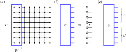
Figure 4: Contraction of a 2D tensor network. One proceeds by blocking columns (blue box in panel (a)). The resulting block $\psi$ is then approximated by a 1D tensor network, i.e., an MPS, with bond dimension $\chi$ (panel (b)). In order to keep the truncation error in all iterations small, it is necessary that the correlations between the upper and lower part of $\psi$ are bounded, i.e., the singular value decomposition in the $A$ vs. $B$ partition has a small tail (shown in panel (c) across the central cut, where we expect most correlations.) This weight can be assessed by whether the entropy across the cut scales with the width $W$. By choosing $H/2$ sufficiently larger than $W$, we ensure that solely $W$ bounds the possible correlations. Concretely, we choose $H/2=2W$; we have found that further increasing $H$ does not lead to an increase in correlations.

In practice, tensor networks are not contracted using Monte Carlo sampling. Rather, in the case of e.g. a 2D lattice as in our case, one proceeds by contracting the tensor network column-wise, where the contracted column tensor $\psi$ is itself again approximated by a 1D tensor network (“boundary MPS”) with a limited bond dimension $\chi$. This procedure is illustrated in Fig. 4a,b and further elaborated on in the caption. In order to obtain an accurate boundary MPS approximation, it is necessary that the Schmidt coefficients of the boundary tensor $\psi$ across all cuts decay rapidly, in a way where the truncation error does not depend (or only weakly depends) on the width $W$ (where by analogy, we treat the contracted region as a quantum state $\psi$ which we normalize)—this ensures an efficient scaling of $\chi$, and thus the computational cost, as the system size (and thus $W$) increases. In particular, we generally expect an efficient scaling in $W$ if the entanglement across a cut is constant or grows at most logarithmically in $W$, while a faster growth speaks against such an approximation; see also Ref. [16].

IV.1 Numerical results

We have performed numerical studies to see whether the entanglement in the boundary state $\psi$ in the PEPS contraction exhibits a hardness transition when moving towards positive tensor networks. To this end, we have computed the $2$-Rényi entropy

$$S_{2}(\psi)=-\log\frac{\mathrm{tr}_{A}\big{[}(\mathrm{tr}_{B}\,\lvert\psi\rangle\langle\psi\rvert)^{2}\big{]}}{\mathrm{tr}\big{[}\lvert\psi\rangle\langle\psi\rvert]^{2}}$$ (5)

for a contracted region of width $W$ and a cut in the center of the tensor network, where we expect the entropy to be largest, see Fig. 4a,c. Here, $\psi$ labels the tensor for the region, see Fig. 4b, which we can interpret as an (unnormalized) bipartite quantum state $\lvert\psi\rangle$ between systems $A$ and $B$. To ensure that $W$ limits the entanglement between $A$ and $B$, rather than than $H/2$ (the size of the systems $A$ and $B$), we chose $H/2=2W$; we have checked that the entropy does not grow when $H$ is increased even further.

The results are shown in Fig. 5. Panels a,b,c show data obtained for different values of $W$ and different bond dimensions $D$. The different panels differ by the scaling of the $y$ axis, which we discuss momentarily, while the $x$ axis for all three panels is $\lambda D$.

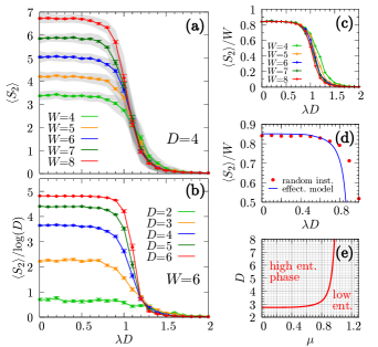
Figure 5: Entanglement (as measured by the $2$-Rényi entropy) of the boundary state $\psi$, Fig. 4a (with $H=4W$), encountered in entanglement-based contraction of a random tensor network with shifted Haar-orthogonal tensors, Eq. (3). (a) Average entanglement $\langle S_{2}\rangle$ vs. $\lambda D$ for different widths ($D=4$). An increasingly sharp transition from a regime with large entanglement to one with vanishing entanglement is observed around $\lambda D=1$. The grey stripes indicate the interval in which typical instances (one sigma) lie; the error bars are the standard deviation of the average. (b) Rescaled entanglement $\langle S_{2}\rangle/\log(D)$ vs. $\lambda D$ for different values of $D$ ($W=6$). The plot confirms that the transition happens at constant $\lambda D\approx 1$, independent of the value of $D$ (with the exception of $D=2$, which does not exhibit a transition; see text), and is compatible with an expected $S_{2}\propto\log\,D$ scaling in the highly entangled phase. (c) Same data as in (a), but with a rescaled $y$ axis $\langle S_{2}\rangle/W$, which clearly confirms a $S_{2}\propto W$ scaling in the highly entangled phase; it also shows more clearly how the transition becomes increasingly sharp as $W$ increases. (d) Comparison of $\langle S_{2}\rangle/W$ with the values predicted by the statmech model. Given that the statmech model only reproduces the randomness average correctly in the large-$D$ limit, the data agrees remarkably well (except that the statmech model exhibits a sharper transition). (e) Phase diagram as predicted by the statmech model. Note that the statmech model does not predict a hard phase for $D=2$ even for $\lambda=0$ (i.e., Haar-distributed tensors with mean $0$), which is in agreement with the behavior seen in (b), as well as previous observations [17, 18].

The plots clearly show a transition in entanglement, and thus a hardness transition in the entanglement-based contraction. What is remarkable, however, is that the transition happens at constant $\lambda D$, roughly around $\lambda D\approx 1$, which becomes evident in Fig. 5b, which compares data for different $D$ (with the exception of the $D=2$ case, which we will return to later).

The fact that the transition occurs at a displacement $\lambda\approx 1/D$ of the Haar-random (or Gaussian) distribution comes as quite a surprise. Both intuitively and from the analysis in the previous section, we would have expected the transition to occur at a constant value of $\lambda$, independent of $D$, that is, when the entries of the tensors become predominantly positive. Instead, at $\lambda=1/D$, the probability of a positive entry is only roughly $1/2+1/\sqrt{2\pi}D$, barely biased away from a symmetric distribution, and the distribution is becoming more and more symmetric as $D$ is being increased.

Leaving the surprising transition point aside, the entanglement scales as expected: The collapse in Fig. 5c (with $S_{2}/W$ on the $y$ axis) shows that the entropy in the hard (highly entangled) phase is proportional to $W$, and Fig. 5b (with $y$ axis $S_{2}/\log D$) is consistent with convergence to an $S_{2}\propto\log D$ scaling—both are consistent with the maximum possible value $W\log D$ for the entanglement. In the easy (weakly entangled) phase, we observe (not shown) that the data for different $W$ collapses, and decays roughly exponentially with $\lambda$, with a slight $D$-dependence of the decay. Finally, let us point out an interesting transition in the distribution of $S_{2}$ over different random instances for fixed $D$, $W$, and $\lambda$: While in the hard phase, $\exp(S_{2})$ follows a Gaussian distribution (which is natural, given that $S_{2}$ is a logarithmic quantity), in the easy phase $\log(S_{2})$ (!) is Gaussian distributed. The latter in particular implies that the distribution of $S_{2}$ has long tails, and the true average of $S_{2}$ might be somewhat larger; at the same time, it raises the question whether the randomness average is really the most meaningful quantity to study as opposed to, say, the median. Finally, let us point out that the same transition is also observed in other entropies, in particular also those with Rényi index smaller than one, as well as for the von Neumann entropy.

Overall, we are left with the puzzling fact that the entanglement transition from hard (volume-law entangled) to easy (boundary-law entangled) happens at a displacement $\lambda$ of the random distribution (3) of the tensor which scales as $\lambda\approx 1/D$, and thus a very slight bias of the distribution towards positive entries is already sufficient to reduce the entanglement and make the task of tensor network contraction tractable on average.

IV.2 Randomness average and effective model

To shed more light on the transition observed in the entanglement, and the location of the transition point at constant $\lambda D$, we study the average behavior of the $2$-Rényi entropy, Eq. (5), of the tensor $\psi$, cf. Fig. 4, where the average is taken over random choices of all the tensors $A^{(s)}$ which make up $\psi$—that is, we will consider

$$\langle S_{2}\rangle=\int\prod_{s}\mathrm{d}U^{(s)}S_{2}(\psi)\ ,$$ (6)

where the average $\langle\,\cdot\,\rangle$ is over Haar-random $U$ in Eq. (3). In what follows, we focus on the real-valued Haar-orthogonal distribution; see Sec. IV.3 and Appendix B for the Haar-unitary case.

In our analysis, we will concentrate on the limit where $D$ is large. In that regime, there is a concentration of measure, that is, the fluctuations about the average become small rapidly [19]. This has two important consequences: First, the typical values, i.e., those which occur with high probability, will get increasingly closer to the average entropy $\langle S_{2}\rangle$. Second, the fact that fluctuations vanish implies that in Eq. (5), we can take the average of the numerator and denominator separately, that is, we can rewrite $\langle S_{2}\rangle$ as

$$\big{\langle}S_{2}(\psi)\big{\rangle}\approx-\log\frac{\big{\langle}\mathrm{tr}_{A}\big{[}(\mathrm{tr}_{B}\,\lvert\psi\rangle\langle\psi\rvert)^{2}\big{]}\big{\rangle}}{\big{\langle}\mathrm{tr}\big{[}\lvert\psi\rangle\langle\psi\rvert]^{2}\big{\rangle}}\ .$$ (7)

where the equation becomes exact as $D\to\infty$.

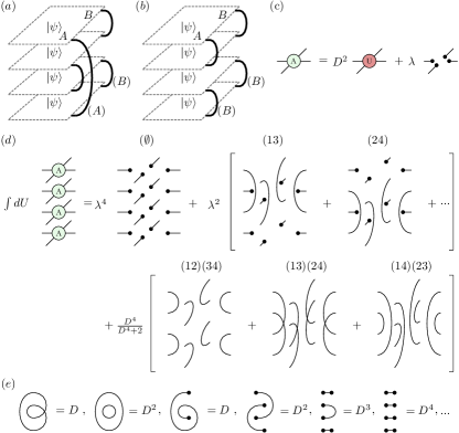
Figure 6: Construction of the statistical mechanics model for the average entanglement, Eq. (7). Numerator and denominator are evaluated separately; for either of them, four copies of $\psi$ are required. (a) Boundary conditions for the numerator in (7), amounting to tracing $B$ on twice two copies, squaring, and tracing $A$. (b) Normalization in the denominator. (c) Tensor used [cf. (3)], which is a sum of a Haar-random tensor and the constant all-$1$ tensor. (d) The Haar-average over $4$ copies of the tensor $A$ contains terms with none, two, and four Haar-random terms $U$ [cf. panel (c)], respectively, resulting in all possible ways to pair up the corresponding copies. This gives in total $10$ configurations which can be associated to each site with corresponding weights $\lambda^{4}$, $\lambda^{2}$, and $D^{4}/(D^{4}+2)$. (e) Given two configurations at adjacent sites, their contraction gives rise to an overlap pattern of loops and all-$1$ tensors, with some examples shown, where each closed loop or open string evaluates to $D$.

Let us now first consider the Haar-average of the numerator. (We will see later that the analysis of the denominator only differs by boundary conditions.) Computing $\mathrm{tr}_{A}\big{[}(\mathrm{tr}_{B}\,\lvert\psi\rangle\langle\psi\rvert)^{2}\big{]}$ requires taking four copies of $\lvert\psi\rangle$, $\lvert\psi\rangle\langle\psi\rvert\otimes\lvert\psi\rangle\langle\psi\rvert$ (since for now, we work with real-valued tensors, we need not worry about conjugates), where suitable boundary conditions—shown in Fig. 6a—implement the partial traces and the square. Since at each site, the average is over the individual Haar-random $U^{(s)}$, we have to consider

$$\int\mathrm{d}UA_{x^{1}}\otimes A_{x^{2}}\otimes A_{x^{3}}\otimes A_{x^{4}}\stackrel{{\scriptstyle\eqref{eq:A-shifted-orthogonal}}}{{=}}\lambda^{4}\ +$$ (8)

$$\lambda^{2}D^{4}\int\mathrm{d}U\,U_{x^{1}}\otimes U_{x^{2}}+\dots+$$

$$D^{8}\int\mathrm{d}U\,U_{x^{1}}\otimes U_{x^{2}}\otimes U_{x^{3}}\otimes U_{x^{4}}\ ,$$

where now $x^{k}=(x^{k}_{\ell}x^{k}_{r}x^{k}_{u}x^{k}_{d})$ are the indices of the tensor in the $k$’th layer, and the middle term includes all $\genfrac{(}{)}{0.0pt}{1}{4}{2}=6$ positions for the $U_{x^{k}}\otimes U_{x^{\ell}}$; the odd terms vanish in the integral. The integrals can be evaluated using Weingarten calculus [20, 21]: Each integral with two $U$’s at $k$ and $k^{\prime}$ yields $\delta_{x^{k}x^{k^{\prime}}}/D^{4}$; while the righmost integral evaluates to

$$\frac{1}{D^{4}(D^{4}+2)}\left(\delta_{x^{1}x^{2}}\delta_{x^{3}x^{4}}+\delta_{x^{1}x^{3}}\delta_{x^{2}x^{4}}+\delta_{x^{1}x^{4}}\delta_{x^{2}x^{3}}\right)$$ (9)

(recall that the dimension of each index $x^{k}$ is $D^{4}$). We can now represent these different terms in the integrals at each site as configurations $\sigma^{(s)}$ of a classical spin (over which we sum), which is associated to each site. This spin $\sigma^{(s)}$ thus takes configurations

$$1\equiv(\emptyset),\ \{\delta_{ij}\equiv(ij)\},\ \{\delta_{ij}\delta_{kl}\equiv(ij)(jk)\}\ ,$$

that is, it takes $10$ configurations per site (namely $1$, $6$, and $3$ configurations for the three groups above, respectively). These configurations are shown in Fig. 6d. Each of these configurations is assigned a weight from the prefactor in Eq. (8) (equivalently, in Fig. 6d). In addition, contracting the indices between two adjacent vertices $s$ and $s^{\prime}$ in all layers assigns a weight to each link which depends on the values of the corresponding $\sigma(s)$ and $\sigma(s^{\prime})$; specifically, each open or closed line/loop in the overlap gives a factor $D$, as illustrated in Fig. 6e.

The randomness average thus maps the four copies of the tensor network to the partition function of a statistical mechanics model

$$\sum_{\{\sigma^{(s)}\}}e^{-\left[\sum_{s}h(\sigma^{(s)})+\sum_{\langle s,s^{\prime}\rangle}k(\sigma^{(s)},\sigma^{(s^{\prime})})\right]}\ ,$$ (10)

with one- and two-body terms $h$ and $k$ which depend on $\lambda$ and $D$; we return to their specific form in a moment.

In order to compute the Haar-average of $\mathrm{tr}_{A}\big{[}(\mathrm{tr}_{B}\,\lvert\psi\rangle\langle\psi\rvert)^{2}\big{]}$, we still need to impose suitable boundary conditions, which can be realized by coupling an additional column of spins in a fixed configuration via $k(\sigma,\sigma^{\prime})$ to the spins at the boundary. In region $B$ (cf. Fig. 4c), those spins are in state $(12)(34)\equiv(B)$, while in region $A$, they are in state $(23)(14)\equiv(A)$, see Fig. 6a. In the same vein, the normalization can be obtained by imposing boundary condition $(B)$ everywhere. (Note that $(A)$ and $(B)$, as well as $(C)\equiv(13)(24)$, are related by permuting copies, so any choice will do.) In principle, we also need to modify the on-site weights $\exp[-h(\sigma^{(s)})]$ for the spins at the other boundaries to account for the missing tensor legs, but the precise nature of those boundaries becomes less important as we increase the system size, as will become clear when we discuss the mechanism behind the transition.

What is the form of the Hamiltonian terms $h$ and $k$? The derivation, and its precise form, are given in Appendix A. What is central for our derivation is that (after rescaling each tensor by $A^{(s)}\to A^{(s)}/D$), $e^{-k(\sigma,\sigma^{\prime})}=\delta_{\sigma,\sigma^{\prime}}+O(1/\sqrt{D})$, that is, the system becomes ferromagnetic in the large-$D$ limit. At the same time, $h(\sigma)$ only depends on $\lambda D\eqqcolon\mu$ (together with a weak $D$-dependence of $O(1/D^{4})$ which vanishes rapidly as $D\to\infty)$. This immediately confirms what we observed in Fig. 5b, namely that the transition happens around constant $\lambda D=\mu$—it is the only parameter left in the effective model.

So how does changing $\mu$ induce a transition in the system? Tuning $\mu$ determines which configurations are favored by the on-site term $h$ in the Hamiltonian. For $\mu<1$, $h$ favors the subspace with the three configurations $(A)$, $(B)$, and $(C)$. Since the interaction $h(\sigma,\sigma^{\prime})$ is ferromagnetic, this means that the system exhibit symmetry breaking (or, maybe more precisely, long-range order) in the subspace given by these three configurations. That is, up to fluctuations, the spins at all sites want to be in the same state—either $(A)$, $(B)$, or $(C)$. We now need to impose the relevant boundary conditions $(A)$ and $(B)$ in the lower and upper half of the system, respectively (Fig. 6a). This will force the lower half of the system to be in state $(A)$, and the upper half in state $(B)$, and will thus give rise to a domain wall between the lower and upper half. This domain wall will incur an energy penalty proportional to its length, implying an exponential decay of the twisted-boundary partition function $\mathrm{tr}_{A}\big{[}(\mathrm{tr}_{B}\,\lvert\psi\rangle\langle\psi\rvert)^{2}\big{]}$. The length scale $\xi$ of the decay depends on the strength of the ferromagnetic interaction $k(\sigma,\sigma^{\prime})$ (i.e., on $D$, where $\xi\to 0$ as $D\to\infty$). At the same time, the denominator has the same boundary condition in both regions, and thus does not face such an exponential suppression. Thus, the average Rényi entropy (which is minus the logarithm of the above quantity) will increase linearly with the length of the domain wall. The length of the shortest (and thus most favorable) domain wall is $W$, and thus, for $\mu<1$ we expect a linear growth of the entropy in $W$.

For $\mu>1$, on the other hand, $h(\sigma)$ uniquely prefers the configuration $(\emptyset)$, and due to the ferromagnetic coupling, the system will be (approximately) in the state $(\emptyset)$, and thus disordered. In particular, this implies that the twisted $(A)$–$(B)$ boundary conditions, Fig. 6a, will give rise to a finite value, independent of $W$. (The precise value will again depend on the strength of the ferromagnetic interactions, that is, on $D$, and vanish as $D\to\infty$.)

We have simulated the phase diagram of the effective statmech model using infinite MPS (see Appendix A for details). The phase diagram is shown in Fig. 5e, where for large $D$, we can distinguish a symmetry-broken high entanglement phase for $\mu\lesssim 1$, and a symmetric low entanglement phase for $\mu\gtrsim 1$. For smaller $D$, the high-entanglement phase shrinks, and eventually disappears for $D\approx 2.73$—this suggests that contracting random tensor networks with $D=2$ is easy on average, and only becomes hard as $D\geq 3$. While this has to be taken with care, as our analysis relies on concentration of measure arguments which only become accurate for large $D$, this is consistent with what we observed in Fig. 5b, as well as with previous findings on entanglement in Haar-random tensor networks (i.e. along the line $\mu=0$), where (with a different technique to capture non-integer bond dimensions) a transition just above $D=2$ had been found [18].

Let us note that the statmech mapping equally applies to other other lattices or graphs, including higher-dimensional lattices. The resulting model only depends on the coordination number $\kappa$ of the lattice, and is obtained from the model above by replacing $D$ by $D^{\kappa/4}$; in particular, in a regular lattice in $\mathcal{D}$ dimensions, it predicts a transition at $\lambda\approx 1/D^{\mathcal{D}/2}$.

IV.3 Unitary ensemble

We have carried out the same analysis—both the study of random instances and the derivation and study of the effective statmech model—also for the complex Haar-random ensemble in Eq. (3). The findings match those reported in the previous subsections; in particular, the transition is observed at constant $\lambda D$, which can be explained from the effective statmech model obtained from the randomness average, which for large $D$ again exhibits a local term which only depends on $\lambda D$, together with a diverging ferromagnetic coupling. For details, see Appendix B.

IV.4 Positive vs. factorizing tensor networks

How can we better understand this transition in the entanglement? One attempt towards an explanation could be to interpret (3) as an interpolation

$$A^{(s)}_{(x_{\ell}x_{r}x_{u}x_{d})}=D^{2}U^{(s)}_{(x_{\ell}x_{r}x_{u}x_{d})}+\lambda S_{(x_{\ell}x_{r}x_{u}x_{d})}$$ (11)

between the Haar-random tensor $D^{2}U^{(s)}$ and a tensor $S_{x_{\ell}x_{r}x_{u}x_{d}}\equiv 1$. We can now write the tensor network as a sum of terms with either $A$ or $S$ at any site, with a prefactor $\lambda^{s}$ (where $s$ is the number of times $S$ occurs). Clearly, as $\lambda$ increases, terms with more $S$ will dominate. Since $S$ has tensor rank 1, i.e., is of product form

$$S_{x_{\ell}x_{r}x_{u}x_{d}}=v^{\ell}_{x_{\ell}}v^{r}_{x_{r}}v^{u}_{x_{u}}v^{d}_{x_{d}}\ ,$$ (12)

placing an $S$ at a vertex will “cut apart” the tensor network at that vertex. For a large enough density of $S$ (on the order of one), we would thus expect a percolation-type transition which would (in typical instances) decouple the tensor network into efficiently contractible pieces. We could then e.g. try to contract the network by sampling over the distribution of $A$ vs. $S$. At the same time, a realization with many $S$ will have a small amount of entanglement, and it is not implausible that this property persists even when superimposing all such configurations.

This picture offers a few appealing features, and could potentially give rise to alternative sampling-based contractions. It is, however, far from rigorous – neither do we know that the sampling does not have a sign problem, nor is it clear that the fact that most individual realizations of $A$ vs. $S$ tensors have low entanglement is reflected in the entanglement of the overall state. At the same time, it suggests interesting connections to e.g. measurement-based induced phase transitions [22, 23, 24, 25, 26], where probabilistic (or otherwise weak) measurements induce an entanglement transition in the output of a quantum circuit, related to an underlying percolation transition.

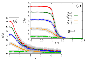
Figure 7: Average entanglement ($2$-Rényi entropy $S_{2}$) for the interpolation to different tensors, cf. Eq. (11). (a) Interpolation to a tensor $S$ with rank $1$, but both positive and negative entries: The transition is now at constant $\lambda$, independent of $D$, consistent with a percolation argument, see text. (Specifically, $v^{\ell}$ and $v^{u}$ in (12) are chosen to have the same number of $+1$ and $-1$ entries, up to rounding, such that the overlaps of two adjacent $S$ yield balanced positive and negative values; note that the sign pattern of the entries of $S$ is only relevant up to rotations on the bonds.) (b) Interpolation to a randomly chosen site-independent tensor $S$ (not rank-$1$) with positive entries (chosen uniformly at random between $0$ and $2$). The same transition behavior as in Fig. 5 is observed: The transition is much sharper than in panel (a), and occurs at a constant value of $\lambda D$, i.e., $\lambda\propto 1/D$.

If this argument were valid, however, this raises a crucial question: What is the role of positivity? After all, the argument we just gave should apply to any rank-$1$ state $S$ [Eq. (12)], even if it is not positive-valued; and conversely, it does not apply to non-factorizing positive $S$. Fortunately, this can be easily tested numerically, with the result shown in Fig. 7 (see caption for details).

Specifically, Fig. 7a shows the entanglement vs. $\lambda$ for an interpolation to a rank-$1$ tensor $S$ with both positive and negative entries. We observe that—unlike in Fig. 5b—(i) there is no sharp transition, but rather a relatively smooth decrease in the entanglement (and, e.g., the tails have much larger entropy), and (ii) the cross-over in the entanglement happens around $\lambda\sim 1$, rather than $\lambda=1/D$ (observe the similarity between the curves for different $D\geq 3$). Indeed, this is consistent with the percolation argument, whose transition depends on the density of $S$, and thus the value of $\lambda$, independent of $D$. Still, it is noteworthy that it is at a value of $\lambda$ on the order of $1$ where the entanglement starts to vanish, which is where we also observed a corresponding behavior for $\Delta f$ (Fig. LABEL:fig:free-energy), even though in the current case, the transition does not seem to depend on positivity, in contrast to the the transition seen in $\Delta f$.

This shows that for the entanglement transition observed around $\lambda=1/D$ for the interpolation (12), it is central that we are interpolating towards positive-valued tensors $S$. But does the tensor also need to be of rank $1$? That this should not be a requirement can already be argued by rewriting Eq. (3) as an interpolation from a Haar-random tensor to a mixture of a Haar-random tensor and the identity, by shifting part of $U$ into $S$—the resulting model will still have a transition at a value of $\lambda$ which scales with $1/D$ (depending on the amount shifted). To substantiate this further, we have also studied an instance where we interpolate towards a fixed random positive tensor $S$ at each site, shown in Fig. 7b; just as in Fig. 5, we observe (i) a sharp transition, and (ii) at a fixed value of $\lambda D\approx 1$.

The effect of interpolating towards non-positive rank-$1$ tensors $S$ can also be studied once again through a randomness average. To this end, we replace $S$ in Eq. (12) by a Haar-random rank-$1$ tensor (i.e., a product of $4$ Haar-random tensors). The randomness average gives once again rise to a statmech model, which we analyze in Appendix C, and which confirms our observations.

V PEPS expectation values and completely positive tensor networks

In variational PEPS simulations, the tensor networks one needs to contract generally arise as a normalization or as expectation values of local observables. They thus have a very special structure, in that each tensor $A^{(s)}$ in the 2D tensor network is obtained by contracting the corresponding PEPS tensor $C^{(s),i}_{y_{\ell}y_{r}y_{u}y_{d}}$ and its adjoint through their physical index $i=1,\dots,d$ (with $d$ the physical dimension per site), that is,

$$A^{(s)}_{x_{\ell}x_{r}x_{u}x_{d}}=\sum_{i}C^{(s),i}_{y_{\ell}y_{r}y_{u}y_{d}}\bar{C}^{(s),i}_{z_{\ell}z_{r}z_{u}z_{d}}$$ (13)

(see Fig. 9a), where the double-layer index $x_{\bullet}=(y_{\bullet},z_{\bullet})$, $\bullet=\ell,r,u,d$, has dimension $D^{2}$ for a PEPS with bond dimension $y_{\bullet}=1,\dots,D$. The tensors $A^{(s)}$ of the resulting 2D tensor network thus do not in general have positive entries (unless they are obtained from PEPS with positive entries). They do, however, come with another type of positivity: When interpreted as a map from ket to bra indices, they amount to positive semidefinite operators, i.e., they can be written in the form (13) (i.e., “$C^{\dagger}C$” acting from ket to bra) for some $C^{(s)}$. Equally, the evaluation of physical observables can be decomposed as a sum of two such positive semidefinite objects. This raises the question whether this positivity structure can still ease the computational difficulty of the contraction. In the following, we will address this question through the various tools introduced in the preceding sections.

V.1 Randomness average

First, we can map the problem to a statmech model, by taking Haar-random tensors $C^{(s)}$ and taking the randomness average of four copies of the resulting 2D tensor network defined by $A^{(s)}$ [Eq. (13)], which amounts to $\big{\langle}(C^{(s)}\otimes\bar{C}^{(s)})^{\otimes 4}\big{\rangle}$. In the given situation, the restriction to real-valued $C^{(s)}$ seems less motivated, and we thus focus on Haar-random unitary tensors $C^{(s)}$. The resulting Haar-average is a sum over all permutations $\pi\in S_{4}$ of four copies, where each ket degree of freedom in copy $k$ is paired up (through a Kronecker delta) with the corresponding bra degree of freedom in copy $\pi(k)$. The state space per site of the resulting statmech model is thus labelled by permutations $\pi\in S_{4}$.

Now consider a site in state $\pi$. The contracted physical degrees of freedom of the four copies thus form loops corresponding to the cycles of $\pi$; we denote the number of cycles by $c(\pi$). Each closed loop contributes a factor $d$ to the Gibbs weight, and thus, the resulting Hamiltonian is

$$h(\pi)=-\log(d)\,c(\pi)$$ (14)

(corresponding to a Gibbs weight $e^{-h(\pi)}=d^{c(\pi)}$). On the other hand, contracting two adjacent sites in states $\pi_{1}$ and $\pi_{2}$ gives rise to a pattern of closed loops described by the difference $\pi_{1}\pi_{2}^{-1}$ of the two permutations, where now each closed loop contributes a factor $D$; the resulting interaction term in the Hamiltonian is thus given by

$$k(\pi_{1},\pi_{2})=-\log(D)\,c(\pi_{1}\pi_{2}^{-1})\ .$$ (15)

Together, these two terms describe the effective statmech model, cf. Eq. (10). We note that a closely related model for the Gaussian ensemble was derived independently in Ref. [13].

Let us now analyze this model. Clearly, $c(\pi)=4$ for the identity permutation $\pi=\mathrm{id}$, and $c(\pi)\leq 3$ otherwise. In the large $D$ regime, the interaction term (15) thus describes a ferromaget with a $24$-fold degenerate ground space. For physical dimension $d=1$, the local term $h$ vanishes, and the model therefore exhibits symmetry breaking between the boundary configurations relevant for computing the Rényi entropy (cf. Fig. 6a), which gives rise to a domain wall and as a consequence a linear growth of the entanglement entropy. This is indeed what we should have expected, since for $d=1$, what we study are simply two copies of the same random tensor network with complex entries, for which had already established that it displays a linear growth of entanglement.

What happens when we set $d>1$? Then, the on-site term $h(\pi)=-\log(d)c(\pi)$ will favor the state $\pi=\mathrm{id}$ at each site. This immediately lifts the degeneracy of the ground space, and the system will be in the state $\pi=\mathrm{id}$ at all sites, leading to a breakdown of long-range order. (This is due to the fact that the model was at a first-order transition.) From the analysis of the statmech model we thus expect that, at least for sufficiently large $D$, the problem of contracting PEPS (that is, contracting the double-layer tensor network) will not exhibit a linear growth of entanglement, and should thus scale efficiently again.

V.2 Numerical simulation

This behavior of the entropy is confirmed by numerical simulations of random instances. As shown in Fig. 8a, the entanglement of $\psi$ (Fig. 4) is essentially independent of $W$. Fig. 8b shows the dependence of the entropy (averaged over widths $W=8,\dots,12$) on $d$, where we observe an algebraic decay $S_{2}\propto d^{\alpha}$ (with $\alpha\approx 3$) of the entropy with the dimension of the physical system, while the dependence on the bond dimension $D$ is comparatively minor. The origin of the $d$-dependence will become more clear in the following subsection.

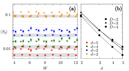
Figure 8: Entanglement scaling for the contraction of PEPS expectation values. Both panels show the average $2$-Rényi entanglement entropy $\langle S_{2}\rangle$ of the boundary state $\psi$, cf. Fig. 4 (for $H=4W$), averaged over $50$ random instances. (a) Dependence of $S_{2}$ on $W$, for different bond dimensions $D$ and physical dimensions $d$; we find that the entanglement does not change with $W$. The grey stripes show the interval for typical (one sigma) values of the entropy for $D=4$. (b) Dependence of $S_{2}$ on the physical dimension $d$ (averaged over $W=8,\dots,12$). We find an algebraic decay with exponent $\alpha\approx 3$; the dependence on $D$ is comparatively weak.

V.3 Expressing PEPS expectation values as a sum of positive terms

In the case of positive-valued tensor networks, we were able to argue that they should be more easily contractible by expressing the contracted value $\mathcal{C}$ as a sum over all classical configurations of the contracted bond variables, Eq. (2). Since each of the terms in the sum was positive, $\mathcal{C}$ could be approximated using Monte Carlo sampling without a sign problem. On a formal complexity theoretic level, applying approximate counting allowed to show that the complexity of approximating $\mathcal{C}$ had a significantly reduced computational complexity. For the current case of contracting PEPS expectation values, the same approach will not work: Sampling over classical configurations of the bonds gives non-positive terms, and sampling over a basis of positive operators $\rho_{i}$ (in the ket-bra partition) instead is not possible since there is no resolution of the identity in terms of only positive operators (the map $\sum\rho_{i}\mathrm{tr}[\sigma_{i}\,\cdot\,]$ with $\sigma_{i},\rho_{i}\geq 0$ is entanglement breaking).

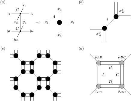
Figure 9: Decomposition of a PEPS expectation value as a sum of efficiently computable positive terms. (a) The two-layer PEPS tensor can be interpreted as tracing out the physical index of a five-partite state $C$, resulting in a mixed state $A$ acting from the ket (bottom) to the bra (top) layer. The right hand side of the equation shows a top view of the double-layer tensor $A$, where the double legs indicate the presence of a ket and bra layer; this notation is also used in the other panels. (b) For large enough dimensions and Haar-random tensor $C$, $A$ is close to the maximally mixed state, and thus has a separable decomposition (dashed line). (c,d) The separable decompositions are chosen in alternating partitions, such as to form small loops. The value of such a loop can be efficiently computed, and is always positive (as it is the overlap $\mathrm{tr}[(\rho_{AB}\otimes\sigma_{CD})(\tau_{AD}\otimes\mu_{BC})]$ of two positive operators). Instead of loops, other efficiently contractible structures such as strings or trees also work fine. Throughout the argument, density operators act between ket and bra indices.

Yet, as we show in the following, it is possible to rewrite the contraction $\mathcal{C}$ of a PEPS expectation value as a sum of positive terms, which can in turn be evaluated by sign-problem-free Monte Carlo sampling, and allows for the application of approximate counting to reduce the complexity from #P to BPP${}^{\textsf{NP}}$; the argument works with probability approaching one for sufficiently large bond and physical dimension. To this end, observe that the single-site double-layer tensor $A^{(s)}$ can be interpreted as a density operator $\rho$ between the ket and the bra layer of the tensor network, which is obtained from a Haar-random state $C^{(s)}$ by tracing out the physical index (i.e., contracting it with its adjoint, Fig. 9a). If we further group the tensor legs into two groups of two (e.g. left+down vs. up+right, Fig. 9b), we can think of $\rho$ as a bipartite mixed state $\rho_{AB}$ defined on a Hilbert space of dimension $D^{2}\times D^{2}$, which is obtained from a Haar-random pure state of dimension $d\times D^{2}\times D^{2}$ by tracing out the $d$-dimensional system. We can now combine two facts: First, if we trace a large enough part of a high-dimensional Haar-random state, the remaining state $\rho_{AB}$ is close to the identity [27]; and second, if a state is sufficiently close to the identity, it is separable [28], i.e.,

$$\rho_{AB}=\sum p_{i}\sigma_{A}^{i}\otimes\sigma_{B}^{i}\ ,$$ (16)

with $\sigma_{\bullet}^{i}\geq 0$ and $p_{i}>0$; see Fig. 9b for an illustration. More specifically, this transition occurs when $d\sim D^{6}$ [29], with probability approaching $1$ as $D\to\infty$. Moreover, the decomposition (16) can be constructed efficiently in the dimension of the space [28].

We can now place such a separable decomposition of the tensor $A^{(s)}$ at each vertex, where we choose the bipartition such that the grouped indices form squares, cf. Fig. 9c. Let us now choose a specific value $i_{k}$ in the sum for the separable decomposition (16) at each site. Then,

$$\mathcal{C}=\sum_{i_{1},\dots,i_{N}}T(i_{1},\dots,i_{N})\ ,$$ (17)

where the value $T(i_{1},\dots,i_{N})$ is obtained by multiplying the overlaps of the separable decompositions, which can be calculated individually across every other plaquette. For each plaquette, this value is of the form $\mathrm{tr}[(\rho_{AB}\otimes\sigma_{CD})(\tau_{AD}\otimes\mu_{BC})]$ (see Fig. 9d), which is an overlap of two positive semidefinite operators and thus itself non-negative. We thus find that the contraction $\mathcal{C}$ of the tensor network can be expressed as an exponentially big sum over efficiently computable positive terms. Therefore, it can be efficiently approximated using Monte Carlo sampling without a sign problem, and approximate counting implies that it can be approximated with a much lower computational complexity.

The fact that for $d\gg D^{4}\gg 1$ a Haar-random tensor becomes close to maximally entangled between virtual and physical indices is equivalent to saying that the PEPS tensor (as a map from virtual to physical indices) gets close to an isometry. This means that the PEPS approaches a state which simply consists of maximally entangled bonds between adjacent sites, with no non-trivial map acting on them (that is, a Projected Entangled Pair State without a projection). One can then immediately see why such a state does not exhibit any entanglement between different regions $A$ and $B$ at the boundary, just as observed in the preceding section.

Let us emphasize that we do not expect to be able to obtain a positive sum decomposition for the expectation value of every PEPS, as there is an intrinsic gap in their worst-case computational complexity: Computing the normalization of a PEPS is a GapP-hard problem (that is, an exponentially big sum with positive and negative weights), or equivalently PostBQP (quantum computing with postselection) [30, 31], which is not expected to be more efficiently approximable, in contrast to exponentially big positive sums (i.e., #P) [5]. It remains however an interesting problem for future research to investigate if the above decomposition of a random tensor network into a positive sum can be extended to random tensor networks with any bond dimension, for instance by blocking regions.

The fact that computing the normalization of a random PEPS can be rewritten as a positive sum—in fact, the contraction of a positive tensor network—for sufficiently large dimensions has an interesting consequence: It implies that under this rewriting, the contraction of the PEPS reduces to the contraction of a positive tensor network, which—as we have found in Section IV—does indeed have a favorable entanglement scaling. The above mapping thus provides an additional argument as to why the entanglement-based contraction of PEPS scales nicely despite the presence of non-positive entries: PEPS expectation values are really just positive tensor networks in disguise.

Note that the transformation in Fig. 9 can be interpreted as one step of a kind of tensor network renormalization (TNR) algorithm [32]; it is then an interesting question to further investigate how TNR can be used to remove negative signs in tensor networks, and whether optimizing for positivity provides a viable route towards a stable and efficient application of TNR to the computation of PEPS expectation values (which usually suffers from instabilities due to the dependency on gauge choices [33]).

VI Discussion

In this work, we have considered the hardness of contracting tensor networks, and investigated how it depends on the choice of tensor entries, namely positive entries vs. general real or complex entries. We used complexity theoretic considerations to argue that there must be a transition in the computational complexity of the problem as the sign pattern changes. We then investigated how this “sign problem” would show up in different numerical contraction methods, by considering random tensor networks with entries with mean $\lambda$ and standard deviation $\sigma=1$. On the one hand, we considered contraction by Monte Carlo sampling. There, we found a gradual transition in the hardness of the problem around $\lambda=1$, which is where the tensor entries become predominantly positive. This is in agreement with expectations, and can be seen as a tensor network version of the well-known Quantum Monte Carlo sign problem. On the other hand, we investigated the commonly used contraction method based on boundary MPS. We found that it exhibits a much earlier transition: The entanglement in the boundary state undergoes a transition from volume law to boundary law entanglement scaling already at a mean of $\lambda\approx 1/D$, much earlier than the transition in the Monte Carlo sign problem, and, most surprisingly, earlier for larger $D$. We observed this behavior in the study of random instances, and were able to confirm it through the construction of an effective classical statmech model. We were also able to show that the entanglement transition is governed solely by the shift towards positive entries, and occurs also when interpolating to a correlated random tensor with positive entries. Finally, we investigated the contraction of PEPS expectation values, where we found a boundary law scaling of the entanglement independent of the physical and bond dimension; we subsequently showed that in a certain regime, such a contraction could indeed be rewritten as a positive-valued tensor network, proving its reduced computational complexity, and at the same time providing a direct intuition for the observed entanglement scaling.

Entanglement transitions have been studied in recent years in a variety of contexts. This in particular involves the questions of dynamics and equilibration, such as the MBL transition [34] or entanglement transitions in monitored quantum dynamics, measurement-induced transitions, or other transitions obtained by adding certain non-unitary gates to unitary quantum circuits [22, 23, 24, 25, 26]. Since quantum circuits, including measurements, can be expressed as tensor networks, these systems therefore also provide examples of entanglement transitions in tensor networks. Similarly, entanglement transitions in random tensor networks as a function of the bond dimension $D$ have been investigated previously for random entries with mean $0$ [17, 18] (i.e., the subfamily with $\lambda=0$ of the class we investigated), mimicking non-integer $D$ by a suitable random distribution of bond dimensions; there, an entanglement transition between $D=2$ and $D=3$ has been observed, consistent with our findings.

This illustrates that there is a number of different parameters which can drive entanglement transitions in tensor networks. On the one hand, our results add another axis to it, namely, the positivity of the tensor entries. Yet, there is a profound difference in the nature of the sign problem transition which we observe: The root of this transition is in the fundamentally different computational complexity of the underlying computational problem, and the observed entanglement transition is only one possible way in which this complexity transition manifests itself. In fact, in a forthcoming work, we will show that the same transition also appears in an entirely different contraction algorithm which is inspired by Barvinok’s method for approximating the permanent [35, 36], and which makes no reference to entanglement whatsoever [37]. In this context, a key question which remains to be answered is to determine the true point of the complexity transition, that is, to identify a regime for $\lambda$ where contraction is provably hard.

A related question connects to the QMC sign problem, where the question we posed initially originated from. Our findings do not conclusively answer what happens to the QMC sign problem in tensor networks, i.e., where the intrinsic computational complexity of simulating Hamiltonians with vs. without a sign problem (i.e., QMA-hard vs. stoqMA) shows up in tensor network algorithms. This has several reasons: First, we have focused on random tensor networks, and the tensor networks which appear in numerical simulations are generally not random. (For instance, it is easy to come up with tensor networks with only positive entries with a volume law, by setting indices to be equal such that they form long strings, sometimes termed “rainbow state”.) Second, we have only considered the contraction of tensor networks, as it e.g. arises from iteratively truncating the imaginary time evolution in a simple or full update algorithm, but which does not take into account the computational effort required to find the optimum in variational tensor network algorithms. Finally, as we have observed in Section V, computing expectation values at least for random PEPS has a favorable entanglement scaling again, leaving open the possibility that in variational PEPS simulations, the difficulty of solving a problem with an intrinsic sign problem is entirely in the minimization itself. Understanding what happens to the complexity of a Hamiltonian with an intrinsic QMC sign problem when tackling it with tensor network algorithms thus remains an important open problem. However, one should keep in mind that this question is likely a very hard one, and will depend sensitively on the chosen algorithm, since already in one dimension, it can on the one hand be shown that e.g. certain variants of the variational DMRG algorithm can get stuck in local minima [38, 39], while on the other hand, provably converging algorithms can be devised [40].

Finally, the connections which we established between the positivity of a tensor network, its entanglement scaling, and the hardness of contracting it might also help to develop improved contraction algorithms. In particular, we observed that PEPS contraction has a favorable entanglement scaling, and we also found that the corresponding two-layer tensor network can be transformed into a positive tensor network by a local TNR-like transformation. In turn, we had observed that positive tensor networks have a favorable entanglement scaling and generally a lower computational complexity. This suggests to use positivity of the entries as one guiding principle for how to perform truncations in TNR or other contraction algorithms. Such a truncation should result in tensor networks which can be much more efficiently contracted in the subsequent steps, and thus might very well lead to overall more accurate contractions when compared to methods which minimize the truncation error made in each step individually.

 

Appendix A Detailed discussion of the statmech model obtained from the Haar-orthogonal model

In the following, we provide the details of the statmech model for the randomness average of the Haar-orthogonal model discussed in Sec. IV.2.

We work with the following $10$-state basis for each site (in this order, read line by line):

$$(\emptyset)\;;$$

$$(12),\;(34), (13),\;(24), (14),\ (23)\>;\hskip 71.13188pt$$

$$(12)(34)\>, (13)(24)\>, (14)(23)\ .$$

Note that the three configurations $(12)$, $(34)$, and $(12)(34)$ naturally group together, as do the other two triples (typeset on top of each other). Also note that the model possesses a natural $S_{4}$ symmetry, obtained from permuting the four copies of the tensor network, which acts by conjugation on the cycles $(ij)$ (and thus, in particular, keeps those tripes together).

From Eq. (8) and the expressions for the Haar integrals (Eq. (9) and just above), we immediately obtain the weights for the on-site term

$$\tilde{V}(\sigma)=(\lambda^{4};\ \lambda^{2},\dots;\ D^{4}/(D^{4}+2),\dots)\ .$$ (18)

For the coupling terms, we need to determine the weight obtained from overlapping the loop pattern (i.e., $\delta_{x^{i}x^{j}}$) corresponding to the basis elements. Note that a missing pair $(ij)$ in the first 1+7 basis states amounts to the all-ones tensor, which evaluates to $1$ for every value of $x^{i}$ and $x^{j}$. We thus find that for a given edge, any closed loop or open line contributes a weight $D$ each (cf. Fig. 6e). Carrying out this calculation, we find that the weight associated to a link with adjacent configurations $\sigma$ and $\sigma^{\prime}$ is

$$\tilde{W}(\sigma,\sigma^{\prime})=\sqrt{Q(\sigma)}W(\sigma,\sigma^{\prime})\sqrt{Q(\sigma^{\prime})}\ ,$$ (19)

where $W(\sigma,\sigma^{\prime})=(1/\sqrt{D})^{\tilde{k}(\sigma,\sigma^{\prime})}=e^{-(\log(D)/2)\,\tilde{k}(\sigma,\sigma^{\prime})}$,

$$\tilde{k}=\left[\begin{array}[]{c|cccccc|ccc}0&1&1&1&1&1&1&2&2&2\\ \hline\cr 1&0&2&2&2&2&2&1&3&3\\ 1&2&0&2&2&2&2&1&3&3\\ 1&2&2&0&2&2&2&3&1&3\\ 1&2&2&2&0&2&2&3&1&3\\ 1&2&2&2&2&0&2&3&3&1\\ 1&2&2&2&2&2&0&3&3&1\\ \hline\cr 2&1&1&3&3&3&3&0&2&2\\ 2&3&3&1&1&3&3&2&0&2\\ 2&3&3&3&3&1&1&2&2&0\end{array}\right]$$ (20)

and

$$Q=(D^{4};\ D^{3},\dots;\ D^{2},\dots)\ .$$

We can now absorb the weights $\sqrt{Q(\sigma)}$ into the vertex term $\tilde{V}(\sigma)$ (there are four $\sqrt{Q(\sigma)}$ adjacent to each vertex) to obtain a vertex weight

$$V(\sigma)=D^{4}\times(D^{4}\lambda^{4};\ D^{2}\lambda^{2},\dots;D^{4}/(D^{4}+2),\dots)\ .$$

The prefactor $D^{4}$ amounts to a rescaling of the partition function and can be compensated by rescaling each tensor $A^{(s)}$ by $1/D$. After this rescaling, we find that the randomness average of four copies of the tensor network is equivalent to the partition function of a statmech model with Hamiltonian

$$H({\sigma^{(s)}})=\sum_{s}h(\sigma^{(s)})+\sum_{\langle s,s^{\prime}\rangle}k(\sigma^{(s)},\sigma^{(s^{\prime})})$$ (21)

at inverse temperature $\beta=1$, where

$$h(\sigma)=-(4\log(\lambda D);\ 2\log(\lambda D),\dots;\log\tfrac{D^{4}}{D^{4}+2},\dots)\$$

and

$$k(\sigma,\sigma^{\prime})=\tfrac{\log\,D}{2}\>\tilde{k}(\sigma,\sigma^{\prime})\ ,$$

with $\tilde{k}$ from Eq. (20). Note that $k$ describes a ferromagnetic coupling with additional off-diagonal terms whose Gibbs weights vanish as $D\to\infty$.

Appendix B Results for the Haar-unitary model: Simulation and effective statmech model

In this Appendix, we discuss the tensor network where the tensors are chosen from a shifted Haar-unitary distribution, that is, $U$ in Eq. (3) is chosen from a Haar-random unitary ensemble.

In that case, we can obtain a similar statmech model by replacing the integral on the left hand side of Eq. (8) with the Haar-integral over the unitary group; note that in that case, every second tensor carries a complex conjugate, and thus depends on $\bar{U}$ rather than $U$. Thus, on the right hand side, only integrals involving an equal number of $U$’s and $\bar{U}$’s are non-vanishing. Using Weingarten calculus [20, 21], the integral with one $U$ and $\bar{U}$ evaluates to

$$\int\mathrm{d}U\,U_{x^{1}}\otimes\bar{U}_{x^{2}}=\frac{\delta_{x^{1}x^{2}}}{D^{4}},$$

and the integral with two pairs evaluates to

$$\int\mathrm{d}U\,U_{x^{1}}\otimes\bar{U}_{x^{2}}\otimes U_{x^{3}}\otimes\bar{U}_{x^{4}}$$ (22)

$$= \frac{1}{D^{4}(D^{4}+1)}\left(\delta_{x^{1}x^{2}}\delta_{x^{3}x^{4}}+\delta_{x^{1}x^{4}}\delta_{x^{2}x^{3}}\right).$$

Therefore, for each site, we obtain the 7-state basis

$$(\emptyset),$$

$$(12),(34), (14),(23),\hskip 71.13188pt$$

$$(12)(34), (14)(23)\ .$$

The model differs from the orthogonal group’s statmech model only by the number of basis states and the on-site weights of the $(ij)(kl)$ configurations,

$$\tilde{V}(\sigma)=(\lambda^{4};\ \lambda^{2},\dots;\ D^{4}/(D^{4}+1),\dots)\ .$$ (23)

Carrying out a similar calculation, we correspondingly obtain a coupling weight

$$\tilde{W}(\sigma,\sigma^{\prime})=\sqrt{Q(\sigma)}W(\sigma,\sigma^{\prime})\sqrt{Q(\sigma^{\prime})}\ ,$$ (24)

with $W(\sigma,\sigma^{\prime})=e^{-k(\sigma,\sigma^{\prime})}$,

$$k=\frac{\log\,D}{2}\left[\begin{array}[]{c|cccc|cc}0&1&1&1&1&2&2\\ \hline\cr 1&0&2&2&2&1&3\\ 1&2&0&2&2&1&3\\ 1&2&2&0&2&3&1\\ 1&2&2&2&0&3&1\\ \hline\cr 2&1&1&3&3&0&2\\ 2&3&3&1&1&2&0\end{array}\right]\ ,$$ (25)

and

$$Q=(D^{4};\>D^{3},\dots;\>D^{2},\dots)\ .$$ (26)

After rescaling by $1/D^{4}$ per site, we obtain the partition function of the Hamiltonian (21) at $\beta=1$, with coupling $k(\sigma,\sigma^{\prime})$ from Eq. (25), and local field

$$h(\sigma)=-(4\log(\lambda D);\ 2\log(\lambda D),\dots;\log\tfrac{D^{4}}{D^{4}+1},\dots)\ .$$

We thus find that the model displays again a ferromagnetic coupling $k$, with off-diagonal terms whose Gibbs weights vanish as $D\to\infty$. In the same limit, the local field for $\lambda D<1$ favors the symmetry broken states $(12)(34)$ and $(14)(23)$, corresponding to the two boundary conditions in Fig. 6a, while for $\lambda D>1$, it favors the unique disordered state $(\emptyset)$. This suggests that also the Haar-unitary tensor network should display an entanglement transition around $\lambda D\approx 1$. This is indeed confirmed by numerical simulations for random instances, shown in Fig. 10.

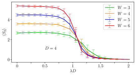
Figure 10: Average $2$-Rényi entropy for the Haar-random unitary model, plotted vs. $\lambda D$ for $D=4$. Just as for the orthogonal case (Fig. 5), we find a transition in the entanglement around $\lambda D\approx 1$.

Appendix C The statmech model of rank-one interpolation

In this Appendix, we follow up on the discussion of the interpolation towards a general (non-positive) rank-$1$ tensor from Sec. IV.4, by deriving an effective statmech model for the interpolation towards rank-$1$ tensors which are chosen randomly at each site. We will focus on the Haar-unitary case, but an analogous discussion applies to the Haar-orthogonal scenario.

To this end, recall that in Sec. IV.4, we considered interpolations of the form (cf. Eq. (12))

$$A^{(s)}_{(x_{\ell}x_{r}x_{u}x_{d})}=D^{2}U^{(s)}_{(x_{\ell}x_{r}x_{u}x_{d})}+\lambda S_{(x_{\ell}x_{r}x_{u}x_{d})}^{(s)}\ ,$$ (27)

where the $S_{(x_{\ell}x_{r}x_{u}x_{d})}^{(s)}$ have rank one,

$$S^{(s)}_{x_{\ell}x_{r}x_{u}x_{d}}=v^{\ell}_{x_{\ell}}v^{r}_{x_{r}}v^{u}_{x_{u}}v^{d}_{x_{d}}\ .$$ (28)

In the following, we will study what happens when all the $v$’s above are chosen independently (for each site $s$ and each direction) at random from the Haar measure. This can be achieved by starting from $S\equiv 1$ in (27) and multiplying each virtual index of $A^{(s)}$ with a Haar-random unitary; since $U^{(s)}$ itself is chosen Haar-random, it remains Haar-random after that transformation, and we have effectively obtained Haar-random $v$’s in (28). When the indices are contracted, we can replace the pair of Haar-random unitaries on the link by a single Haar-random unitary $u$ (for the same reason, the same also applies to open indices at the boundary). Thus, the resulting model differs from the previous one by a term on each link obtained from averaging over $u\otimes\bar{u}\otimes u\otimes\bar{u}$ on the link. Weingarten calculus [20, 21] yields the two configurations $\{(12)(34),(14)(23)\}\eqqcolon\mathcal{T}$ at each side of the link, with corresponding weights

$$Y=\frac{1}{D^{2}-1}\left[\begin{array}[]{cc}1&-\frac{1}{D}\\ -\frac{1}{D}&1\end{array}\right]\ .$$ (29)

The total weight per link can now be conveniently obtained by observing that the resulting loop patterns on the two sides of $Y$ are a subset of those obtained for the unitary model, namely the last two columns (or rows) of $\tilde{W}$ in Eq. (24); let us denote the corresponding $7\times 2$ matrix by $\tilde{W}_{Y}$. The partition function of the statmech model is then obtained by contracting the tensor network with $\tilde{W}_{Y}Y\tilde{W}_{Y}^{T}$ on the links and a weight $\tilde{V}$, Eq. (23), on the vertices.

The fact that the link operator is rank $2$ suggests that the model is most compactly parameterized in terms of Ising (i.e., two-valued) variables on the links. This can be done in two ways: The first option is to split $Y=XX^{T}$ with

$$X=\frac{1}{\sqrt{2(D^{2}-1)}}\begin{bmatrix}1&1\\ 1&-1\end{bmatrix}\begin{bmatrix}\sqrt{\frac{D-1}{D}}&0\\ 0&\sqrt{\frac{D+1}{D}}\end{bmatrix}\ ,$$

which results in a model with Ising variables on the links, coupled by the contraction of $\tilde{V}$ and four times $\tilde{W}_{Y}X$ around each vertex. The resulting model turns out to be an eight-vertex model, though one with a magnetic field, and thus (to our knowledge) not within a class known to be solvable.

A second way to construct a statmech model is to replace $X$ above by the positive square root of $Y$, $Y=R^{2}$ with $R\geq 0$. The resulting model has Ising variables on the link, and a Gibbs weight $T(i,j,k,l)$ on every vertex (with $i,j,k,l=0,1$ the surrounding link variables) which only depends on the number of $1$’s,

$$T(i,j,k,l)=w(i+j+k+l)\ .$$

and where $w(0)=w(4)$, $w(1)=w(3)$. Specifically, after dividing out a factor of $D^{4}$ per vertex and up to first order in $1/D$, we have

$$w(0)=w(4) =(1+2\lambda^{2}+\lambda^{4})-2\lambda^{4}\frac{1}{D}+\dots$$ (30)

$$w(1)=w(3) =\lambda^{4}-(2\lambda^{4}-\lambda^{2}-\tfrac{1}{2})\frac{1}{D}+\dots$$ (31)

$$w(2) =\lambda^{4}-2\lambda^{4}\frac{1}{D}+\dots$$ (32)

In addition, the boundary conditions $(A)$ and $(B)$ which we need to impose to compute the 2-Rényi entropy, Fig. 6a, are obtained by applying $R$ to the two canonical basis vectors, and are thus equal to the $0$ and $1$ Ising configuration up to a $1/D$ correction.

Let us now analyze this model. First, for $\lambda=0$ and $D\to\infty$, the only non-zero terms are $w(0)=w(4)=1$, that is, the model is an Ising ferromagnet. For finite but large $D$, we find that in addition, $w(1)=w(3)=1/2D$. The corresponding tensors can be used to construct a domain wall interfacing the boundary conditions $(A)\equiv 0$ and $(B)\equiv 1$, Fig. 6a; this gives rise to a finite cutoff of the entropy, just as seen in Fig. 7a at $\lambda=1$. Since the probability for any of those interface tensors is $1/2D$, and the length of the domain wall scales linearly with $W$, we expect a scaling of the entropy proportional to $W\log D$ for sufficiently large $D$.

Let us next see what happens when we increase $\lambda$, where we will take $D\to\infty$. Then, we can split $T(i,j,k,l)$ as follows: It is a sum of (i) a ferromagnetic term with weight $1+\lambda^{2}$, and (ii) an equal weight mixture of all 16 configurations, that is, a paramagnetic (disordered) system, with weight $\lambda^{4}$. We then expect the domain wall between the $(A)$ and the $(B)$ boundary to break down if the disordered tensors (suitably normalized) percolate and thus separate the two boundaries. Naturally, this should happen for a ratio of weights $\tau=\lambda^{4}/(1+\lambda^{2})$ on the order of $1$; this is indeed consistent with the observed behavior where the transition in entropy is at a fixed $\lambda$, independent of $D$.

References

- Becca and Sorella [2017] F. Becca and S. Sorella, Quantum Monte Carlo Approaches for Correlated Systems (Cambridge University Press, 2017).
- Bañuls [2023] M. C. Bañuls, Tensor Network Algorithms: A Route Map, Annual Review of Condensed Matter Physics 14, 173 (2023), arXiv:2205.10345 .
- Barahona [1982] F. Barahona, On the computational complexity of Ising spin glass models, J. Phys. A 15, 3241 (1982).
- Troyer and Wiese [2005] M. Troyer and U.-J. Wiese, Computational Complexity and Fundamental Limitations to Fermionic Quantum Monte Carlo Simulations, Phys. Rev. Lett. 94, 170201 (2005), arXiv:cond-mat/0408370 .
- Stockmeyer [1983] L. Stockmeyer, The complexity of approximate counting, in Proceedings of the fifteenth annual ACM symposium on Theory of computing - STOC ’83, STOC ’83 (ACM Press, 1983).
- Kempe et al. [2006] J. Kempe, A. Kitaev, and O. Regev, The Complexity of the Local Hamiltonian Problem, SIAM Journal of Computing 35, 1070 (2006), quant-ph/0406180 .
- Bravyi et al. [2008] S. Bravyi, D. P. DiVincenzo, R. I. Oliveira, and B. M. Terhal, The Complexity of Stoquastic Local Hamiltonian Problems, Quant. Inf. Comput. 8, 361 (2008), quant-ph/0606140 .
- Gharibian et al. [2015] S. Gharibian, Y. Huang, Z. Landau, and S. W. Shin, Quantum Hamiltonian Complexity (2015).
- Jordan et al. [2008] J. Jordan, R. Orus, G. Vidal, F. Verstraete, and J. I. Cirac, Classical simulation of infinite-size quantum lattice systems in two spatial dimensions, Phys. Rev. Lett. 101, 250602 (2008), cond-mat/0703788 .
- Jiang et al. [2008] H. C. Jiang, Z. Y. Weng, and T. Xiang, Accurate determination of tensor network state of quantum lattice models in two dimensions, Phys. Rev. Lett. 101, 090603 (2008), arXiv:0806.3719 .
- Verstraete and Cirac [2004] F. Verstraete and J. I. Cirac, Renormalization algorithms for Quantum-Many Body Systems in two and higher dimensions, (2004), cond-mat/0407066 .
- Gray and Chan [2024] J. Gray and G. K.-L. Chan, Hyper-optimized approximate contraction of tensor networks with arbitrary geometry, Phys. Rev. X 14, 011009 (2024), 2206.07044v2 .
- Gonzalez-Garcia et al. [2023] S. Gonzalez-Garcia, S. Sang, T. H. Hsieh, S. Boixo, G. Vidal, A. C. Potter, and R. Vasseur, Random insights into the complexity of two-dimensional tensor network calculations (2023), 2307.11053 .
- Grover and Fisher [2015] T. Grover and M. P. A. Fisher, Entanglement and the Sign Structure of Quantum States, Phys. Rev. A 92, 042308 (2015), 1412.3534v1 .
- Hangleiter et al. [2020] D. Hangleiter, I. Roth, D. Nagaj, and J. Eisert, Easing the Monte Carlo sign problem, Science Advances 6, 10.1126/sciadv.abb8341 (2020), arXiv:1906.02309 .
- Schuch et al. [2008a] N. Schuch, M. M. Wolf, F. Verstraete, and J. I. Cirac, Entropy scaling and simulability by Matrix Product States, Phys. Rev. Lett. 100, 30504 (2008a), arXiv:0705.0292 .
- Vasseur et al. [2019] R. Vasseur, A. C. Potter, Y.-Z. You, and A. W. W. Ludwig, Entanglement transitions from holographic random tensor networks, Phys. Rev. B 100, 134203 (2019), arXiv:1807.07082 .
- Levy and Clark [2021] R. Levy and B. K. Clark, Entanglement Entropy Transitions with Random Tensor Networks, (2021), arXiv:2108.02225 .
- Hayden et al. [2016] P. Hayden, S. Nezami, X.-L. Qi, N. Thomas, M. Walter, and Z. Yang, Holographic duality from random tensor networks, Journal of High Energy Physics 2016, 9 (2016), arXiv:1601.01694 .
- Collins [2003] B. Collins, Moments and cumulants of polynomial random variables on unitary groups, the Itzykson-Zuber integral, and free probability, Int. Math. Res. Not. 17, 953 (2003), arXiv:math-ph/0205010 .
- Collins and Matsumoto [2009] B. Collins and S. Matsumoto, On some properties of orthogonal Weingarten functions, Journal of Mathematical Physics 50, 113516 (2009), arXiv:0903.5143 .
- Skinner et al. [2019] B. Skinner, J. Ruhman, and A. Nahum, Measurement-Induced Phase Transitions in the Dynamics of Entanglement, Phys. Rev. X 9, 031009 (2019), arXiv:1808.05953 .
- Napp et al. [2022] J. Napp, R. L. L. Placa, A. M. Dalzell, F. G. S. L. Brandao, and A. W. Harrow, Efficient classical simulation of random shallow 2D quantum circuits, Phys. Rev. X 12, 021021 (2022), 2001.00021v2 .
- Chan et al. [2019] A. Chan, R. M. Nandkishore, M. Pretko, and G. Smith, Unitary-projective entanglement dynamics, Phys. Rev. B 99, 224307 (2019), arXiv:1808.05949 .
- Bao et al. [2020] Y. Bao, S. Choi, and E. Altman, Theory of the phase transition in random unitary circuits with measurements, Phys. Rev. B 101, 104301 (2020), arXiv:1908.04305 .
- Ippoliti et al. [2021] M. Ippoliti, M. J. Gullans, S. Gopalakrishnan, D. A. Huse, and V. Khemani, Entanglement Phase Transitions in Measurement-Only Dynamics, Phys. Rev. X 11, 011030 (2021), arXiv:2004.09560 .
- Hayden et al. [2006] P. Hayden, D. W. Leung, and A. Winter, Aspects of Generic Entanglement, Commun. Math. Phys. 265, 95–117 (2006), arXiv:quant-ph/0407049 .
- Braunstein et al. [1999] S. L. Braunstein, C. M. Caves, R. Jozsa, N. Linden, S. Popescu, and R. Schack, Separability of Very Noisy Mixed States and Implications for NMR Quantum Computing, Phys. Rev. Lett. 83, 1054–1057 (1999), arXiv:quant-ph/9811018 .
- Aubrun et al. [2013] G. Aubrun, S. J. Szarek, and D. Ye, Entanglement Thresholds for Random Induced States, Communications on Pure and Applied Mathematics 67, 129–171 (2013), arXiv:1106.2264 .
- Schuch et al. [2007] N. Schuch, M. M. Wolf, F. Verstraete, and J. I. Cirac, The computational complexity of PEPS, Phys. Rev. Lett. 98, 140506 (2007), quant-ph/0611050 .
- Aaronson [2005] S. Aaronson, Quantum Computing, Postselection, and Probabilistic Polynomial-Time, Proc. R. Soc. Lond. A 461, 3473 (2005), quant-ph/0412187 .
- Evenbly and Vidal [2015] G. Evenbly and G. Vidal, Tensor Network Renormalization, Phys. Rev. Lett. 115, 180405 (2015), arXiv:1412.0732 .
- [33] M. C. Bañuls, private communication.
- Nandkishore and Huse [2015] R. Nandkishore and D. A. Huse, Many body localization and thermalization in quantum statistical mechanics, Annual Review of Condensed Matter Physics 6, 15 (2015), 1404.0686v2 .
- Barvinok [2016] A. Barvinok, Computing the permanent of (some) complex matrices, Foundations of Computational Mathematics 16, 329 (2016), arXiv:1405.1303 .
- Eldar and Mehraban [2018] L. Eldar and S. Mehraban, Approximating the permanent of a random matrix with vanishing mean, in 2018 IEEE 59th Annual Symposium on Foundations of Computer Science (FOCS) (IEEE, 2018) pp. 23–34, arXiv:1711.09457 .
- [37] J. Jiang et al., in preparation.
- Eisert [2006] J. Eisert, Computational Difficulty of Global Variations in the Density Matrix Renormalization Group, Phys. Rev. Lett. 97, 260501 (2006), arXiv:quant-ph/0609051 .
- Schuch et al. [2008b] N. Schuch, I. Cirac, and F. Verstraete, The computational difficulty of finding MPS ground states, Phys. Rev. Lett. 100, 250501 (2008b), arXiv:0802.3351 .
- Landau et al. [2015] Z. Landau, U. Vazirani, and T. Vidick, A polynomial time algorithm for the ground state of one-dimensional gapped local Hamiltonians, Nature Phys. 11, 566 (2015), arXiv:1307.5143 .