Associating LOFAR Galactic Faraday structures with the warm neutral medium

Faraday tomography observations with the Low Frequency Array (LOFAR) have unveiled a remarkable network of structures in polarized synchrotron emission at high Galactic latitudes. The observed correlation between LOFAR structures, dust polarization, and $\mathsc{H\,i}$ emission suggests a connection to the neutral interstellar medium (ISM). We investigated this relationship by estimating the rotation measure (RM) of the warm neutral (partially ionized) medium (WNM) in the local ISM. Our work combines UV spectroscopy from FUSE and dust polarization observations from Planck with LOFAR data. We derived electron column densities from UV absorption spectra toward nine background stars, within the field of published data from the LOFAR two-meter sky survey. The associated RMs were estimated using a local magnetic field model fitted to the dust polarization data of Planck. A comparison with Faraday spectra at the position of the stars suggests that LOFAR structures delineate a slab of magnetized WNM and synchrotron emission, located ahead of the bulk of the warm ionized medium. This conclusion establishes an astrophysical framework for exploring the link between Faraday structures and the dynamics of the magnetized multiphase ISM. It will be possible to test it on a larger sample of stars when maps from the full northern sky survey of LOFAR become available.

1 Introduction

New telescopes, instruments, and sky surveys in low-frequency radio astronomy (Wayth et al., 2015; Shimwell et al., 2017; Wolleben et al., 2019; Shimwell et al., 2019, 2022) are poised to greatly expand studies of the diffuse interstellar medium (ISM). Rotation measure (RM) synthesis emphasizes the information encoded in the observations by distinguishing polarized emission along the line of sight (LoS) based on the Faraday rotation it has undergone (Brentjens & de Bruyn, 2005; Van Eck, 2018). This data analysis technique, which provides data cubes of polarized intensity versus Faraday depth, is referred to as Faraday tomography. The data cubes reveal an unexpected structural richness in the polarized Galactic synchrotron emission that offers information on the 3D structure of interstellar magnetic fields and electrons (Iacobelli et al., 2013; Jelić et al., 2014, 2015; Lenc et al., 2016; van Eck et al., 2017; Thomson et al., 2019; Van Eck et al., 2019; Turić et al., 2021; Erceg et al., 2022). When interpreting the data, we are faced with our limited understanding of the ionization of the diffuse ISM and, in particular, with the difficulty in identifying the ISM component to which the Faraday structures relate.

Correlation with ISM tracers provides clues on the nature of Faraday features. Comparison of LOFAR observations with Planck maps have revealed a tight correlation between the orientation of structures in Faraday data and the magnetic field component in the plane of the sky traced by dust polarization in a few mid-latitude Galactic fields located in the surroundings of the extragalactic point source 3C 196 (Zaroubi et al., 2015; Jelić et al., 2018; Turić et al., 2021). LOFAR structures have also been observed to correlate with $\mathsc{H\,i}$ filaments associated with the cold neutral medium (Kalberla & Kerp, 2016; Kalberla et al., 2017; Jelić et al., 2018) and, more generally, with maps of ISM phases (cold, unstable and warm gas) derived from the analysis of $\mathsc{H\,i}$ spectral data cubes (Bracco et al., 2020). The observational results are limited because the published data comparisons focus on a few fields close together in the sky. However, they point to a common physical framework in which the LOFAR structures trace the neutral dusty ISM, and not the warm ionized medium (WIM). To test this hypothesis, we present this work in which we estimate the RM associated with the warm neutral medium (WNM) in the local ISM.

The UV spectroscopic data in absorption toward background stars indicate that the ionization fraction of the WNM is about 0.1, in the thick Galactic disk (Spitzer & Fitzpatrick, 1993), the local ISM (Jenkins, 2013) and small clouds of warm gas embedded within the Local Bubble (LB, Redfield & Falcon, 2008), in particular the local interstellar cloud encompassing the Sun (Slavin & Frisch, 2008; Gry & Jenkins, 2017; Bzowski et al., 2019)). The WNM, rather than the WIM (Reynolds et al., 1998), could be the specific ISM component traced by low-frequency Faraday observations at high Galactic latitude, as proposed by Heiles & Haverkorn (2012) and van Eck et al. (2017), and supported by the numerical simulations presented by Bracco et al. (2022).

This work brings together the analysis of the LOFAR Two-meter Sky Survey (LoTSS, Shimwell et al., 2022), the mosaic at high latitudes toward the outer Galaxy analyzed by Erceg et al. (2022), with UV spectroscopy and dust polarization observations. We combine electron column densities derived from UV spectroscopic observations toward stars with a model of the local magnetic field fitted on Planck dust polarization maps to estimate the RM of the WNM in the local ISM. The comparison with Faraday spectra on the same LoS allows us to assess the WNM contribution to the Faraday rotation of the polarized synchrotron emission measured by LOFAR.

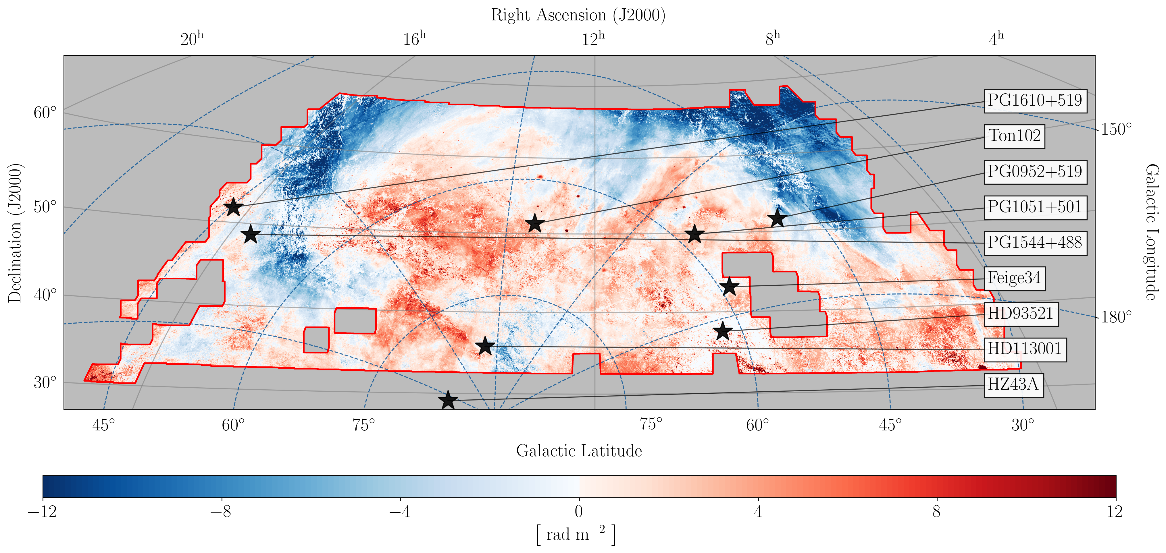
Figure 1: Stars in our sample overlaid on a LOFAR image of the LoTSS field from Erceg et al. (2022). The image displays the first moment of the Faraday spectra in units of ${\rm rad\leavevmode\nobreak\ m^{-2}}$. Celestial and Galactic coordinates are plotted with solid and dashed lines, respectively.

The paper is organized as follows. We introduce stellar targets and present the UV observational data in Sect. 2. The model of the local magnetic field that we use to estimate the RM from electrons in the WNM is presented in Sect. 3 and Appendix A. The comparison with LOFAR observations is presented in Sect. 4. Our work brings a new perspective to the interpretation of LOFAR Faraday data: the origin of the structures and the contribution from the WIM, which we discuss in Sect. 5. The main results are summarized in Sect. 6.

Table 1: Stellar targets and results of the data fit

Star	$l$	$b$	parallax	d	log($N{(\mathsc{O\,i}})$)	b	[$\mathsc{A{\rm r}\,i}$/$\mathsc{O\,i}$]
	∘	∘	mas	pc	cm-2	km s—1
	(a)		(b)	(c)			(d)
HZ43A	54.106	84.162	$16.6\pm 0.05$	$60.3\pm 0.2$	$14.49\pm 0.05$	$2.9\pm 0.3$	$-0.52\pm^{0.24}_{0.41}$
PG1544+488	77.539	50.129	$1.99\pm 0.04$	$497\pm 9$	$16.42\pm{0.07}$	$11.1\pm{0.6}$	$-0.45\pm{0.06}$
PG1610+519	80.506	45.314	$0.94\pm 0.04$	$1040\pm^{40}_{30}$	$16.76\pm{0.08}$	$19.5\pm{0.8}$	$-0.70\pm{0.09}$
HD113001	110.965	81.163	$7.3\pm 0.6$	$140\pm^{20}_{10}$	$16.42\pm 0.10$	$9.7^{0.8}_{0.7}$	$0.23\pm^{0.40}_{0.36}$
Ton102	127.051	65.775	$1.07\pm 0.03$	$920\pm 30$	$16.30\pm^{0.38}_{0.24}$	$5.8^{2.1}_{1.5}$	$-0.37\pm^{0.44}_{0.37}$
PG1051+501	159.612	58.120	$0.73\pm 0.04$	$1350\pm^{80}_{70}$	$16.72\pm^{0.40}_{0.26}$	$12.6\pm^{2.6}_{2.0}$	$0.24\pm^{0.39}_{0.32}$
PG0952+519	164.068	49.004	$1.70\pm 0.05$	$580\pm 20$	$16.12\pm{0.05}$	$13.3\pm^{0.7}_{0.6}$	$-0.54\pm{0.06}$
Feige 34	173.315	58.962	$4.36\pm 0.10$	$227\pm 5$	$15.88\pm^{0.33}_{0.24}$	$6.4\pm^{4.1}_{2.3}$	$-0.40\pm^{0.43}_{0.51}$
PG1032+406	178.877	59.010	$4.67\pm 0.05$	$212\pm 2.5$	$15.93\pm^{0.30}_{0.26}$	$6.7\pm^{2.2}_{1.6}$	$-0.26\pm 0.85$
HD93521	183.140	62.152	$0.78\pm 0.08$	$1250\pm^{150}_{100}$	$16.46\pm 0.08$	-	$-0.48\pm 0.11$

a: Galactic coordinates.
b: Gaia eDR3 parallax.
c: Median value of the distance posterior with $1\,\sigma$ uncertainty from the catalog of Bailer-Jones et al. (2021).
d: Abundance ratio normalized to the solar value.

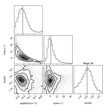
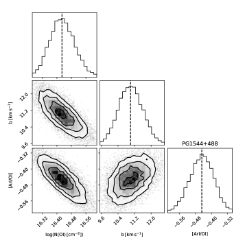
Figure 2: Corner plots of MCMC data fit for two stars in our sample Feige 34 (left) and PG1544+488 (right), chosen as examples of low and high column densities. The histograms show the probability distribution of the three model parameters, and the contours display their interdependence. The dashed lines plotted over the histograms represent the median values of the model parameters.

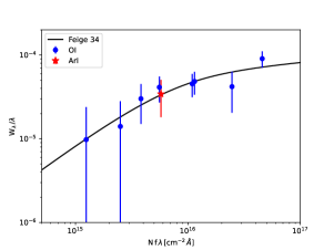
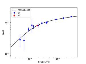
Figure 3: Curves of growth for the two stars Feige 34 (left) and PG1544+488 (right), chosen as examples of low and high column densities. For each graph, the y-axis represents the ratio between the equivalent width, W_λ, and the wavelength, $\lambda$, of the line, and the x-axis the product of the column density N expressed in cm^-2, the strength of the transition (unit-less f-value), and $\lambda$ in Å. The blue circles represent the equivalent widths of the $\mathsc{O\,i}$lines used to determine the column density of $\mathsc{O\,i}$ and the Doppler parameter, $b$, and the red star the equivalent width of the $\mathsc{A{\rm r}\,i}$ line used to determine the [$\mathsc{A{\rm r}\,i}$/$\mathsc{O\,i}$] abundance ratio.

2 Stellar targets and data

We introduce our sample of stellar targets with spectroscopic UV observations in Sect. 2.1. Our analysis of the UV spectra is presented in Sect. 2.2. In Sect. 2.3, the results of our data fitting are used to derive column densities of electrons in the WNM.

2.1 Spectroscopic UV observations

To build this project, we searched scientific publications for UV spectroscopic observations, at high Galactic latitudes over the sky area covered by the LOFAR Faraday tomography mosaic (hereafter the LoTSS field) analyzed by Erceg et al. (2022). We obtained a sample of nine stellar sources. This sample includes eight stars from the study of Jenkins (2013) plus the halo star HD 93521 (Spitzer & Fitzpatrick, 1993). To this set, we added the star HZ43A (Kruk et al., 2002), which lies close to the edge of the LoTSS field. This star, located $60\,$pc from the Sun, allows us to probe the contribution of the very nearby gas in this region of the sky.

In Fig. 1, the stellar positions are overlaid on an image of the first moment of the Faraday data cube from Erceg et al. (2022), representing the polarized intensity-weighted mean of Faraday spectra in units of ${\rm rad\leavevmode\nobreak\ m^{-2}}$. All stars have been observed with the Far Ultraviolet Spectroscopic Explorer (FUSE) with a spectral resolution $R\equiv\nu/\Delta\nu\simeq 2\times 10^{4}$.

Stellar coordinates and data relevant to this study are listed in Table 1. The parallaxes and corresponding distances are from the Gaia data release eDR3 (Lindegren et al., 2021). The column densities of $\mathsc{A{\rm r}\,i}$ and $\mathsc{O\,i}$ are inferred from the FUSE UV spectra. We follow Jenkins (2013) using the [$\mathsc{A{\rm r}\,i}$/$\mathsc{O\,i}$] column density ratio, normalized to Solar abundances, to estimate the ionization fraction of the WNM. The ionization potentials of $\mathsc{A{\rm r}\,i}$ and $\mathsc{H\,i}$ are close, but the photo-ionization cross section of $\mathsc{A{\rm r}\,i}$ is much larger. The ionization fraction of $\mathsc{O\,i}$ is strongly locked to that of $\mathsc{H\,i}$ through a strong charge-exchange reaction. These two factors make [$\mathsc{A{\rm r}\,i}$/$\mathsc{O\,i}$] a sensitive tracer of $\mathsc{H\,i}$ ionization in the WNM (Sofia & Jenkins, 1998). Since neutral forms of argon and oxygen are virtually absent in fully ionized regions (either the prominent $\mathsc{H\,ii}$ regions around hot stars or the much lower density but more pervasive WIM), our probes sample only regions that have appreciable concentrations of $\mathsc{H\,i}$. This sets our measurements apart from conventional determinations of average electron densities (e.g. pulsar dispersion measures, H_α line intensity, $\mathsc{C\,ii}$ fine-structure excitation), which are strongly influenced by contributions from fully ionized gas.

2.2 Data analysis

The column densities of $\mathsc{O\,i}$ and $\mathsc{A{\rm r}\,i}$ (number of absorbing atoms in a column of unit cross-section along the LoS) are determined by a curve of growth analysis (Strömgren, 1948; Draine, 2011). The curve of growth relates the gas column densities of the absorbers, $N$, to the strength of absorption lines measured by their equivalent width $W_{\lambda}$ (normalized area of the line expressed in wavelength units). The function $W_{\lambda}(N)$ is computed assuming that the absorbers have a Gaussian velocity distribution characterized by the Doppler width $b=\sqrt{2}\times\sigma_{v}$, where $\sigma_{v}$ is the velocity dispersion. By fitting the equivalent widths of multiple lines of different strength one can infer the two parameters $N$ and $b$ from the data.

We used the equivalent widths of multiple $\mathsc{O\,i}$ lines and a single $\mathsc{A{\rm r}\,i}$ line, measured by Jenkins (2013), and by Kruk et al. (2002) for HZ43A. The oscillator strengths of the lines are listed in these two papers. The fit of the curve of growth is performed with three free parameters: the column density $N(\mathsc{O\,i})$ of $\mathsc{O\,i}$ atoms, the abundance ratio [$\mathsc{A{\rm r}\,i}$/$\mathsc{O\,i}$] normalized to the Solar value, and the Doppler parameter, $b$, of the line profiles, assumed to be the same for $\mathsc{A{\rm r}\,i}$ and $\mathsc{O\,i}$. The spontaneous decay rate that determines the Lorentzian broadening is set to $A=3\times 10^{7}\,$s^-1 ignoring variations among $\mathsc{O\,i}$ states (Morton, 2003). This simplification has no significant impact on the results of our data analysis.

We performed a Monte-Carlo Markov Chain (MCMC) analysis to sample the joint posterior distribution of the three model parameters. We utilize the EMCEE python package as described by Foreman-Mackey et al. (2013) in accordance with their recommendations. We use a Gaussian likelihood and broad priors on the model parameters. We restricted $b$ to values greater than 2 km s^-1 because we consider that in our LoS the $\mathsc{O\,i}$ lines are dominated by warm gas (the partially ionized WNM), which implies a temperature of T $\geq$ 6000 K and, thus, a line broadening $b>2$ km/s. To confirm this hypothesis we looked at the $\mathsc{H\,i}$ 21 cm spectra in direction of each of our stars using the HI4PI data from HI4PI Collaboration et al. (2016) and their Gaussian decomposition by Kalberla & Haud (2018). These data indicate that some of the gas along our LoS is cold but its contribution to the OI absorption lines is minor due to line saturation. The cold neutral medium (CNM) could contribute to very weak transitions but the $\mathsc{O\,i}$ lines that have the most influence in our analysis have equivalent widths that are not much different from that of the $\mathsc{A{\rm r}\,i}$ line. In this case, comparisons of $\mathsc{A{\rm r}\,i}$ to $\mathsc{O\,i}$ remain valid, and the very narrow components from the CNM have no influence. Moreover, fits to the data for small values of $b$ suppose that the lines are highly saturated and give $\mathsc{O\,i}$ column densities that are incompatible with $\mathsc{H\,i}$ column densities inferred from $\mathsc{H\,i}$ $21\,$cm observations. Figure 2 presents the posterior distributions of the model parameters for two stars Feige 34 and PG1544+488 chosen as examples of low and high column densities of $\mathsc{O\,i}$. The corresponding data fits with the curves of growth are shown in Fig. 3.

The model parameters with their error bars are listed in Table 1. The best estimate is the median value of the posterior distribution, and the negative and positive error bars are computed from the 16 and 84 percentiles. We added to Table 1 data for the star HD 93521. Interstellar matter foreground to HD 93521 has been analyzed in detail by Spitzer & Fitzpatrick (1993). Here, we report the $\mathsc{O\,i}$ column density and the [$\mathsc{A{\rm r}\,i}$/$\mathsc{O\,i}$] abundance ratio that we measured in the FUSE spectra for the low-velocity component. We checked that our estimates of [$\mathsc{A{\rm r}\,i}$/$\mathsc{O\,i}$] are consistent with the values reported by Jenkins (2013) but for PG1610+519. For this parameter of the model, the added value of our data analysis is the posterior distribution that quantifies the interdependence with $N(\mathsc{O\,i})$ and $b$.

Table 2: Column densities and ionization fractions

Star	log$(N({\rm HI}))$	log$(N^{\rm WNM}_{e})$	log$(x_{H})$
	cm-2	cm-2
	(a)	(b)	(c)
HZ43A	$17.73\pm{0.05}$	$16.75\pm_{0.42}^{0.47}$	$0.10\pm_{0.06}^{0.19}$
PG1544+488	$19.66\pm{0.07}$	$18.62\pm{0.17}$	$0.090\pm_{0.020}^{0.024}$
PG1610+519	$20.0\pm{0.08}$	$19.36\pm{0.21}$	$0.23\pm_{0.06}^{0.09}$
HD113001	$19.65\pm{0.10}$	$<18.2$	$<0.035$
Ton102	$19.52\pm_{0.23}^{0.34}$	$18.35\pm_{1.09}^{0.71}$	$0.072\pm_{0.065}^{0.165}$
PG1051+501	$19.93\pm_{0.25}^{0.38}$	$<18.35$	$<0.021$
PG0952+519	$19.36\pm{0.05}$	$18.46\pm{0.14}$	$0.126\pm_{0.024}^{0.03}$
Feige 34	$19.11\pm_{0.23}^{0.31}$	$17.95\pm_{1.56}^{0.76}$	$0.069\pm_{0.066}^{0.215}$
PG1032+406	$19.17\pm_{0.25}^{0.29}$	$17.98\pm_{0.94}^{0.82}$	$0.066\pm_{0.076}^{0.324}$
HD93521	$19.70\pm 0.08$	$18.71\pm_{0.21}^{0.19}$	$0.102\pm_{0.036}^{0.051}$

(a): Log₁₀ of the column density of HI derived from that of OI.
(b): Log₁₀ of the column density of electrons.
(c): Hydrogen ionization fraction.

2.3 Column densities of electrons

The column densities of electrons for the WNM, $N_{e}^{\mathrm{WNM}}$ foreground to the stars are estimated from the results of our fits of FUSE spectra. We follow the approach introduced by Jenkins (2013), to derive the ionization fraction of HI, $x_{\rm H}\equiv n({\rm H}^{+})/n({\mathsc{H\,i}})$, from the [$\mathsc{A{\rm r}\,i}$/$\mathsc{H\,i}$] abundance ratio. We use formula (7) in this paper:

$$[{\mathsc{A{\rm r}\,i}/\mathsc{H\,i}}]={\rm log}\left[\frac{1+x_{\rm H}}{1+P^{\prime}_{\rm Ar}\,x_{\rm H}}\right],$$ (1)

where $P^{\prime}_{\rm Ar}$ is a unit-less parameter, which accounts for various forms of photoionization and recombination with free electrons, as well as additional processes (Jenkins, 2013). [$\mathsc{A{\rm r}\,i}$/$\mathsc{H\,i}$] is deduced from [$\mathsc{A{\rm r}\,i}$/$\mathsc{O\,i}$] for the Solar abundance of oxygen $\rm log[O/H]+12=8.76$. We assume that there is no depletion of oxygen on dust grains, which should be safe for the low-density conditions we are sampling here (Jenkins, 2009). We use $P^{\prime}_{\rm Ar}=22.8$, the value from Table 4 in Jenkins (2013) for a model including ionization by soft X-ray emission from cooling supernova remnants. The statistical distribution of $x_{\rm H}$ is derived from the posterior distribution of [$\mathsc{A{\rm r}\,i}$/$\mathsc{O\,i}$] using Eq. 1, and that of the $\mathsc{H\,i}$ column density $N({\mathsc{H\,i}})$ from $N({\mathsc{O\,i}})$ .

We combine $x_{\rm H}$ and $N({\mathsc{H\,i}})$ values to compute the electron column density:

$$N_{e}^{\rm WNM}=1.2\,x_{\rm H}\,N({\mathsc{H\,i}}),$$ (2)

where the factor 1.2 accounts for electrons from ionized helium, based on the ionization model of the WNM in Jenkins (2013).

The column densities of neutral hydrogen and electrons are listed in Table 2 with their error bars and plotted versus distance in Fig. 4. $N_{e}^{\rm WNM}$ and $N(\mathsc{H\,i})$ seem to be correlated : ¡$N(\mathsc{H\,i})$ / $N_{e}^{\rm WNM}$ ¿ = 10.9 with a small dispersion of 3.6. We observe a tendency for $N$($\mathsc{H\,i}$) to increase with distance but our star sample is too small to draw some firm conclusion about the distance distribution of WNM electrons.

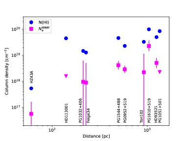
Figure 4: Column densities of HI and WNM electrons. The HI column densities are plotted with blue circles and the electron column densities in the WNM with magenta squares. The two triangles pointing down represent upper limits.

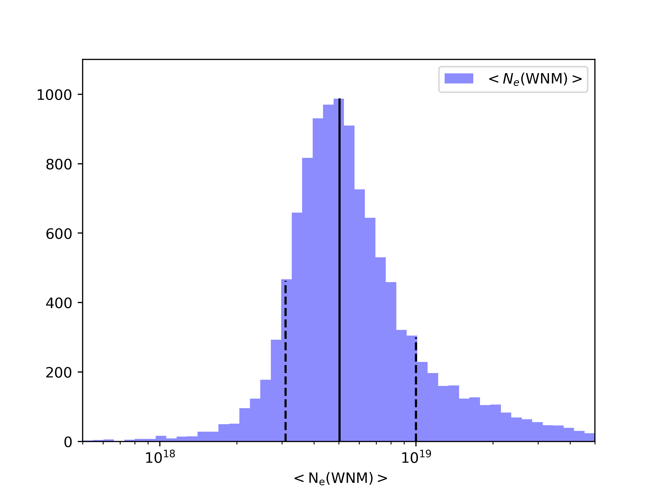
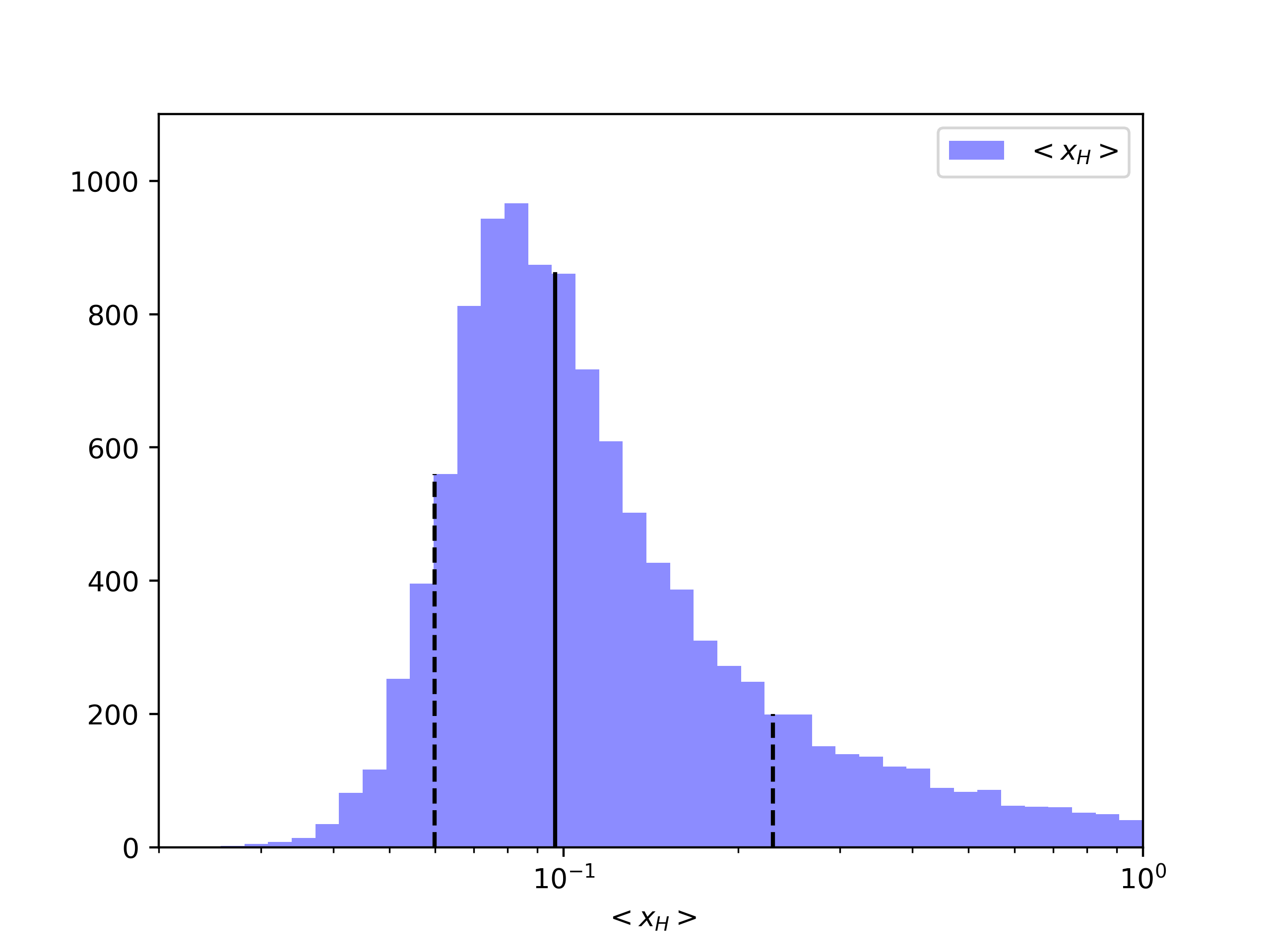
Figure 5: Probability distribution of the mean value of the electron column density (left) and ionization fraction (right). The histograms are built averaging the samples of the posterior distributions over the 9 stars in our sample more distant than 100 pc (i.e. excluding HZ43A). The solid black lines indicate the median value and the dashed lines the 16 and 84% percentiles.

The probability distribution functions (PDFs) of the mean column density of electrons and the ionization fraction averaged over our set of stars are presented in Fig. 5. The PDFs are computed by averaging the samples of the posterior distributions, inferred from our data analysis of UV spectra, over the nine stars in Table 2 more distant than HZ43A. The nearest star in this set is located $140\,$pc from the Sun. The median values for the electron column density and the ionization fraction are $\langle N_{e}^{\mathrm{WNM}}\rangle=5\pm^{5}_{2}\times 10^{18}\,\mathrm{cm}^{-2}$ and $\langle x_{\rm H}\rangle=0.097\pm^{0.133}_{0.037}$, where the lower and upper error bars represent the 16 and 84 percentiles of the distributions. Our median value is consistent with that inferred by Jenkins (2013) from the complete sample of his study. For $P^{\prime}_{\rm Ar}=13.4$, the model value without the contribution of cooling supernovae (Jenkins, 2013), we find $\langle x_{\rm H}\rangle=0.17$. The difference quantifies the dependence of our $x_{\rm H}$ estimates on the choice of ionization model.

The various sources and ionization processes that contribute to the ionization fraction of the WNM are detailed by Jenkins (2013). These include cosmic rays as well as supernova-driven shocks (Sutherland & Dopita, 2017) and soft X-ray emission from cooling supernova remnants (SNRs, Slavin et al., 2000). The degree of ionization of the WNM could also be locally out of equilibrium as an aftereffect of the supernova explosions that have created the LB (Fuchs et al., 2006; Zucker et al., 2022). Within this hypothesis, the WNM ionization could be enhanced around the LB. Analysis of UV data for a larger sample of stars is required to test this hypothesis.

3 Model of the local magnetic field from Planck observations

To estimate the RM from the partially ionized WNM foreground to the stars, we need a model of the magnetic field in the local ISM. The tight correlation between the orientation of Faraday structures in LOFAR data with that of dust polarization (Zaroubi et al., 2015; Jelić et al., 2018) leads us to use the phenomenological model introduced by Planck Intermediate Results XLIV (2016) and Vansyngel et al. (2017) to statistically model dust polarization data at high Galactic latitudes as measured by Planck.

The magnetic field $\@vec{B}$ is expressed as the sum of its mean (ordered) $\@vec{B_{0}}$ and random (turbulent) $\@vec{B_{\rm t}}$ components:

$$\@vec{B}=\@vec{B_{0}}+\@vec{B_{\rm t}}=|\@vec{B_{0}}|\,(\@vec{\hat{B}_{0}}+f_{\rm M}\,\@vec{\hat{B}_{\rm t}}),$$ (3)

where $\@vec{\hat{B}_{0}}$ and $\@vec{\hat{B}_{\rm t}}$ are the unit vectors associated with $\@vec{B_{0}}$ and $\@vec{B_{\rm t}}$, and $f_{M}$ a model parameter that sets the relative strength of the random component of the field. The direction of $\@vec{B_{0}}$ is assumed to be uniform over the sky area used to fit the model parameters. The model also makes the simplifying assumption that the direction of $\@vec{B_{0}}$ does not vary along the LoS. At high Galactic latitudes ($|b|\geq 60^{\circ}$), comparison with stellar polarization data indicates that dust polarization measured by Planck originates mainly from the surroundings of the LB, within about $300\,$pc from the Sun (Skalidis & Pelgrims, 2019). Even if the LOFAR field in Fig. 1 extends to lower latitudes, it is not necessary to account for the structure of the magnetic field across the Galactic disk and into the halo to model Planck dust polarization data over this sky area.

The computational steps taken to determine the magnetic field model are detailed in Appendix A. The direction of $\@vec{\hat{B}_{0}}$ is defined by the Galactic coordinates $l_{0}$ and $b_{0}$, which are derived from a fit of the Planck Stokes $Q$ and $U$ maps at $353\,$ GHz over the sky regions toward the northern Galactic cap comprising the LoTSS field. The random component $\@vec{B_{\rm t}}$ is statistically described using the model of Planck Intermediate Results XLIV (2016) with parameters derived from a fit of the Planck power spectra of dust polarization by Vansyngel et al. (2017). The orientation of $\@vec{B_{\rm t}}$ varies in discrete steps along the LoS over a small number of layers, which schematically represent the correlation length of the turbulent component of the magnetic field. The ratio between $|\@vec{B_{\rm t}}|$ and $|\@vec{B_{0}}|$, $f_{M}=0.9$, is determined fitting Planck power spectra of dust polarization (Vansyngel et al., 2017).

Because the modeling of dust polarization only determines the orientation of the mean magnetic field, we need to use Faraday observations to determine the field strength and also to discriminate between the two opposite directions associated with the orientation. Comparison of the rotation and dispersion measures of pulsars in the northern sky indicates that the mean field strength in diffuse ionized gas in the Galactic disk near the Sun is about 3-$4\,\mu$G (see Table 3 in Sobey et al., 2019). The magnetic field strength in the warm interstellar medium can also be estimated from synchrotron emission. As discussed in Beck et al. (2003), the two estimates differ if fluctuations in magnetic field and electron density are not statistically independent. For the specific objective of the paper, the strength of the mean field estimated from pulsar RMs is a directly relevant reference. We chose this strength $|\@vec{B_{0}}|$ to be ${\bf 3.5}\,\mu$G. The total field strength that includes the turbulent component is $5\,\mu$G.

To estimate the RM from electrons in the WNM, we compute the mean magnetic field component along the LoS, $B_{\mathrm{LoS}}$:

$$B_{\mathrm{LoS}}=-\,(\@vec{B_{0}}+<\@vec{B_{\rm t}}>)\cdot\hat{r},$$ (4)

where $\@vec{B_{\rm t}}$ is averaged over the model layers and $\hat{r}$ is the unit vector defining the LoS. The minus sign makes $B_{\mathrm{LoS}}$ positive when it points toward the Sun. Figure 6 presents our calculation results in the LOFAR field. The top image shows the mean value of $B_{\mathrm{LoS}}$. This map represents $B_{\mathrm{LoS}}$ computed for the mean magnetic field $\@vec{B_{0}}$, ignoring the random component. The bottom image shows $B_{\mathrm{LoS}}$ for one statistical realization of $\@vec{B_{\mathrm{t}}}$. The mean value of $B_{\mathrm{LoS}}$ and the dispersion associated with $\@vec{B_{\rm t}}$ are listed in Table 3.

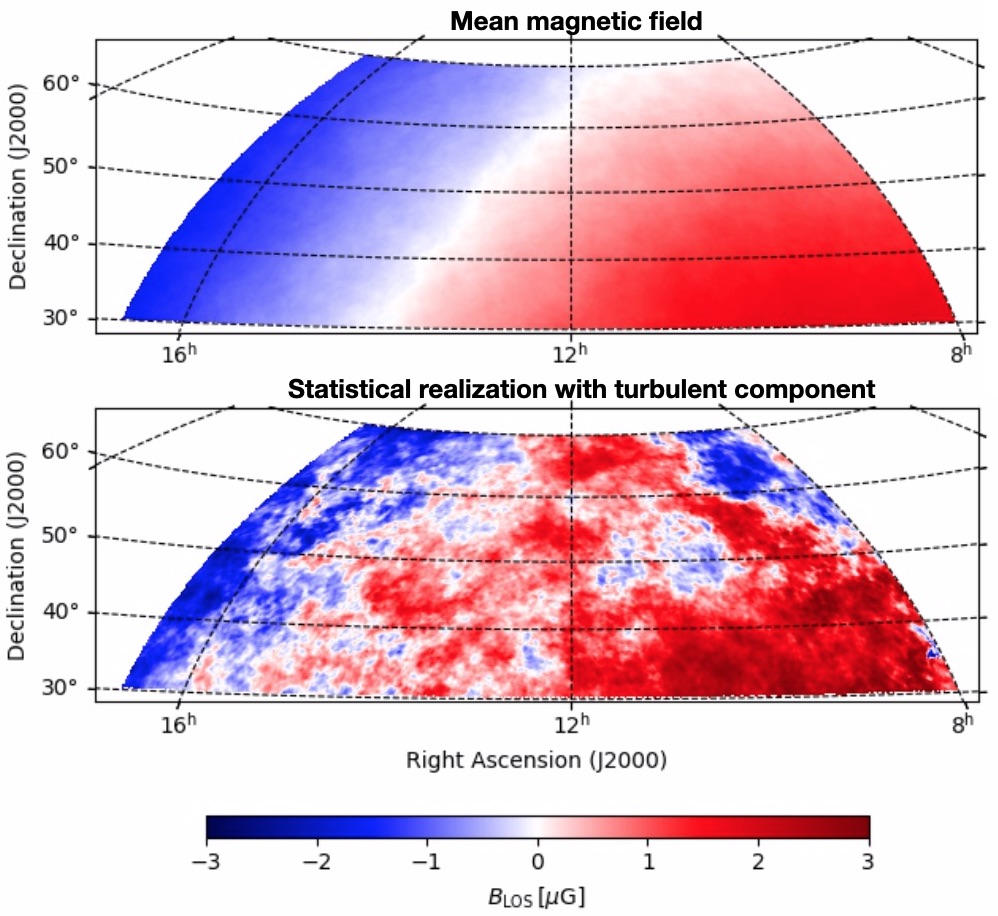
Figure 6: Maps of the magnetic field component along the LoS, $B_{\mathrm{LoS}}$, over the LOFAR field. The top image shows $B_{\mathrm{LoS}}$ for the mean field $\@vec{B_{0}}$ and the bottom image that computed for $\@vec{B}$ including one realization of the turbulent component $\@vec{B_{\rm t}}$. $B_{\mathrm{LoS}}$ is positive when it points toward the Sun (See Eq. 4).

Table 3: $B_{\mathrm{LoS}}$ and WNM RMs

Star	$B_{\mathrm{LoS}}$	RMWNM	$\mathrm{M1_{LOFAR}}$
	$\mathrm{\mu G}$	rad m-2	rad m-2
	(a)	(b)	(c)
HZ43A	$0.49\pm 1.0$	$0.0\pm^{0.02}_{0.01}$	$-$
PG1544+488	$-1.3\pm 0.9$	$-1.4\pm^{1.0}_{1.4}$	$-1.39$
PG1610+519	$-1.5\pm 0.9$	$-8.6\pm^{5.8}_{9.3}$	$0.88$
HD113001	$0.44\pm 1.0$	$0.0\pm{0.2}$	$-0.32$
Ton 102	$0.16\pm 1.0$	$0.0\pm^{1.0}_{0.6}$	$-0.67$
PG1051+501	$0.82\pm 1.0$	$0.0\pm{0.5}$	$-0.46$
PG0952+519	$1.0\pm 0.9$	$0.6\pm^{0.8}_{0.7}$	$-2.02$
Feige 34	$1.2\pm 0.9$	$0.2\pm^{1.4}_{0.2}$	$1.00$
PG1032+406	$1.4\pm 0.9$	$0.2\pm^{2.0}_{0.3}$	$0.0$
HD93521	$1.6\pm 0.9$	$1.7\pm^{2.1}_{1.3}$	$-$

(a) Mean $B_{\mathrm{LoS}}$ inferred from the Planck magnetic field model followed by the standard deviation of the turbulent component B_t.
(b) RM to the star associated with the foreground WNM.
(c) First moment of the LOFAR Faraday spectra. The uncertainty of these values is $1\,\mathrm{rad\,m^{-2}}$.

4 The warm neutral medium and LOFAR Faraday observations

In this section, we assess whether the partially ionized WNM foreground to the stars may account for the LOFAR Faraday spectra. The RMs associated with electrons within the WNM foreground to the stars are determined in Sect. 4.1, and compared with the LOFAR data in Sect. 4.2. Electrons in the WIM are ignored in this section.

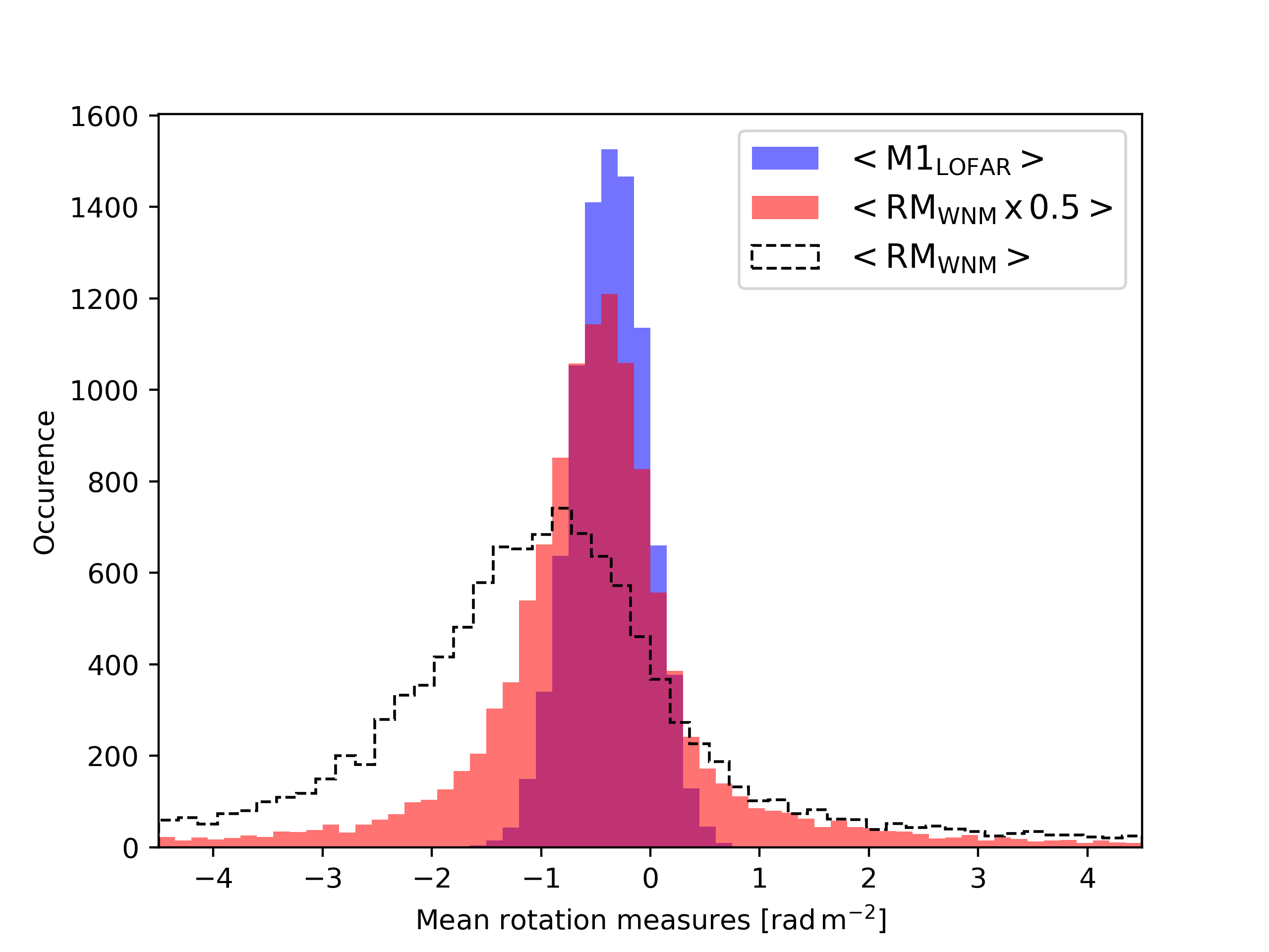
Figure 7: PDFs of the mean RM and the mean LOFAR M1 moment. The plot displays the PDFs of $\langle\mathrm{RM_{WNM}}\times 0.5\rangle$ (red) and $\langle M1_{\mathrm{LOFAR}}\rangle$ (blue). The PDF of $\langle\mathrm{RM_{WNM}}\rangle$ is also shown as a black line. The mean values are computed over the eight stars with both UV and LOFAR data.

4.1 Rotation measures from WNM electrons

The RM to a source at a distance $d$ is defined as

$$\mathrm{RM}(d)=0.812\,{\rm rad\,m^{-2}}\int^{d}_{\rm{0}}\left(\frac{n_{\rm e}}{\rm cm^{-3}}\right)\left(\frac{B_{\parallel}}{\mu{\rm G}}\right)\left(\frac{dl}{\rm pc}\right),$$ (5)

where the integral along the LoS goes from the source at $l=0$ to the observer at $l=d$, $n_{e}$ is the electron density and $B_{\parallel}$ the magnetic field component along the LoS . Using $B_{\mathrm{LoS}}$, the mean value of $B_{\parallel}$ introduced in Eq. 4, we reduce the integral in Eq. 5 to

$$\mathrm{RM_{WNM}}(i)=0.26\,{\rm rad\,m^{-2}}\,\left(\frac{N_{\rm e}^{\rm WNM}(i)}{\rm 10^{18}\,cm^{-2}}\right)\,\left(\frac{B_{\mathrm{LoS}}(i)}{\mu{\rm G}}\right),$$ (6)

where $\mathrm{RM_{WNM}}(i)$ is the RM associated with the column density of electrons $N_{\rm e}^{\rm WNM}(i)$ to the star $i$. Within our statistical model of the magnetic field (Sect. 3), $B_{\mathrm{LoS}}$ for a given LoS has a normal distribution. The mean values and standard deviations of $B_{\mathrm{LoS}}$ are listed for the LoS to the stars in Table 3. The PDF of $B_{\mathrm{LoS}}$ is combined with the posterior distribution of $N_{\rm e}^{\rm WNM}$, inferred from our analysis of the FUSE spectra, to obtain the statistical distribution of $\mathrm{RM_{WNM}}$. The median values of $\mathrm{RM_{WNM}}$ with $1\sigma$ uncertainties are listed in Table 3. These uncertainties are large for all stars because they include the statistical dispersion of the turbulent component of $B_{\mathrm{LoS}}$.

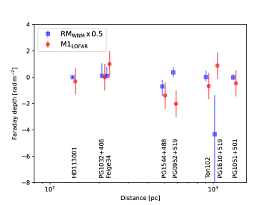
Figure 8: Comparison of the WNM RMs with the first moments of the LOFAR Faraday spectra for each star individually. The values of $\mathrm{RM_{WNM}}\times 0.5$ are plotted with blue squares, and the intensity weighted Faraday depths from LOFAR, $M1_{\mathrm{LOFAR}}$, with red circles.

4.2 Comparison with LOFAR data

We now proceed to the comparison between $\mathrm{RM_{WNM}}$ and the LOFAR data.

The third column of Table 3 lists the first moment of the Faraday spectra for each LoS to the stars. The first moment $\mathrm{M1_{LOFAR}}$ is the mean in Faraday depth of the spectra, weighted by the polarized intensity. The $\mathrm{M1_{LOFAR}}$ values were computed by Erceg et al. (2022) for a polarized intensity threshold of $460\leavevmode\nobreak\ {\rm\mu Jy}$ per angular and Faraday resolution elements. No values could be measured for HD 93521 because the polarized emission at this position is too weak to be detected. HZ43A is just outside the field of the LoTSS field in Fig. 1.

To reduce the uncertainties in the observational data and the statistical dispersion of the turbulent component of the magnetic field, we compared the mean values of $\mathrm{RM}_{WNM}$ and $\mathrm{M1_{LOFAR}}$, computed for the eight stars with the LOFAR values in Table 3. The PDFs of $\langle\mathrm{RM}_{WNM}\rangle$ are computed by combining the statistical distributions of $N_{e}^{\rm WNM}$ and $B_{\mathrm{LoS}}$. The PDF of $\langle\mathrm{M1_{LOFAR}}\rangle$, is calculated from the LOFAR data points using bootstrap statistics (Efron, 1979). We drew thousands of samples of eight values from the data points. Each value in a sample is one of the data points drawn at random, and a given sample may contain the same data point several times. We compute the mean value for each sample. The PDF that we obtain accounts for the data scatter and the sample variance.

In Fig. 7, the PDFs of the mean RM and $\mathrm{M1_{LOFAR}}$ are compared. We discuss this graph in the reference framework introduced by Burn (1966) and consider two idealized cases: (1) a Faraday foreground screen of WNM electrons that rotates the polarization angle of a background synchrotron emission, and (2) a Faraday slab where the polarized synchrotron emission is distributed along the LoS together with the WNM electrons. In the first case, we expect the mean values of $\mathrm{RM_{WNM}}$ and $\mathrm{M1_{LOFAR}}$ to be the same. In the second case, for a symmetric distribution of thermal electrons and polarized synchrotron emission between the near and far sides of the slab, we expect the mean of $\mathrm{RM_{WNM}}$ to be twice that of $\mathrm{M1_{LOFAR}}$ (Sokoloff et al., 1998).

We find a good match between $\langle\mathrm{RM_{WNM}}\times 0.5\rangle$ and $\langle\mathrm{M1_{LOFAR}}\rangle$, which favors case (2). Individual data points for each star are compared and plotted versus distance in Fig. 8. The large error bars on the data points prevent a detailed assessment. We only point out that this plot does not show a systematic trend with distance. The data comparison does not include the systematic uncertainty on electron column densities associated with our choice for $P^{\prime}_{\rm Ar}$ in Sect. 2.3. We note that within the ionization models quantified by Jenkins (2013) the alternative choice for $P^{\prime}_{\rm Ar}$ would produce a mean difference between the WNM RMs and the first moment of the LOFAR spectra greater than a factor of 2.

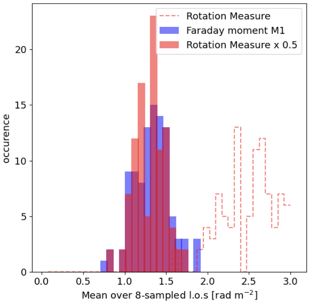
Figure 9: PDFs of the mean RM and the mean LOFAR M1 moments for synthetic observations derived from a numerical simulation by Bracco et al. (2022). The mean values are computed on random sets of eight LoS. The PDFs of $\langle\mathrm{RM_{WNM}}\times 0.5\rangle$ and $\langle M1_{\mathrm{LOFAR}}\rangle$ are plotted in red and blue. The PDF of $\langle\mathrm{RM_{WNM}}\rangle$ is also shown as a dashed line.

Table 4: Data for pulsars within the LoTSS field

Pulsar	$l$	$b$	DM	RM
∘	∘	cm-3  pc	rad m-2
	(a)	(a)	(b)	(c)
B0809+74	139.998	31.618	5.75	-14.00
J0854+5449	162.782	39.408	18.84	-8.8
B0917+63	151.431	40.725	13.15	-14.93
J1012+5307	160.347	50.858	9.02	2.98
B1112+50	154.408	60.365	9.18	2.41
J1434+7257	113.082	42.153	12.60	-9.7
B1508+55	91.325	52.287	19.62	1.5
J1518+4904	80.808	54.282	11.61	-11.9
J1544+4937	79.172	50.166	23.23	9.8

(a): Galactic longitudes and latitudes.
(b): Dispersion measures.
(c): RMs.

5 Insight into the interpretation of LOFAR Faraday data

Our work contributes to a new perspective on the interpretation of LOFAR Galactic polarization data. We discuss two specific questions: the origin of the LOFAR Faraday structures in Sect. 5.1 and the contribution of the WIM in Sect. 5.2.

5.1 Origin of LOFAR Faraday structures

Comparison of the UV and LOFAR data in Fig. 7 suggests that the relativistic electrons producing the synchrotron-polarized emission detected by LOFAR and the thermal electrons in the WNM contributing to Faraday rotation are mixed within the same ISM slab. We take the median value of $\langle\mathrm{RM_{WNM}}\rangle$ as the mean RM across this slab, $\mathrm{RM}_{0}\sim 0.7\,\mathrm{rad\,m}^{-2}$. Because $\mathrm{RM}_{0}$ is smaller than the resolution in Faraday depth of the LoTSS data ($1.2\,\mathrm{rad\,m}^{-2}$), the synchrotron emission from the near and far sides of the slab are not separated through the LOFAR RM-synthesis.

In this context, it is relevant to mention the spatial correlation between polarized dust emission measured by Planckat $353\,$ GHz and the polarized synchrotron emission measured by Planck and WMAP at 30 and $23\,$GHz (Planck Intermediate Results XXII, 2015; Choi & Page, 2015; Planck 2018 results XI, 2020). The correlation coefficient, measured to be approximately 20%, provides an estimate of the fraction of polarized synchrotron emission that comes from the same ISM slab as the WNM, given the tight correlation between dust polarization and $\mathsc{H\,i}$ at high Galactic latitudes (Ghosh et al., 2017; Clark & Hensley, 2019). The remaining 80% of the polarized synchrotron emission would be background to the WNM electrons. We hypothesize that the background emission at LOFAR frequencies undergoes depolarization due to differential Faraday rotation along the LoS. This idea was previously proposed by van Eck et al. (2017) and examined in a separate context by Hill (2018). If this view holds, deep LOFAR observations should reveal weak diffuse polarized emission at higher absolute Faraday depths than the $M1_{\mathrm{LOFAR}}$ values reported by Erceg et al. (2022). Analysis of the LoTSS ELAIS-N1 Deep Field at high Galactic latitude, which combines 150 hours of LOFAR observations, does support this hypothesis. Šnidarić et al. (2023) successfully detected faint Galactic polarized emission at higher absolute Faraday depths, probing the full range of RMs expected from the Galaxy.

Faraday rotation and depolarization produced by a slab of magnetized ISM have been studied analytically by Sokoloff et al. (1998). The polarized emission depends on the relative distribution of the thermal electrons that produce the Faraday rotation and the relativistic electrons that produce the synchrotron emission. Together with the differential Faraday rotation along the LoS, these factors contribute to the variations of the observed polarized intensity. However, this formal framework ignores the bandwidth of the LOFAR observations.

To put the data comparison presented in Fig. 7 into an astrophysical context, we confront our results with those obtained from MHD simulations. To this end, we perform the same comparison between WNM RMs and first moments of Faraday spectra using synthetic observations built from numerical simulations of two colliding shells as input (Ntormousi et al., 2017). We use the synthesized LOFAR maps produced and analyzed by Bracco et al. (2022). Specifically, we use their Case A data where the shells collide in a direction perpendicular to the initial magnetic field for their high value of the cosmic-ray ionization rate $\zeta^{H}=2.6\,10^{-16}\,\mathrm{s}^{-1}$. In these simulations, most of the Faraday rotation occurs within partially ionized WNM gas. The synthesized LOFAR maps have morphological features similar to those revealed by LoTSS data, including depolarization features.

In Fig. 9, we compare the PDFs of the mean RM and the mean first moment, computed on these synthesized LOFAR maps, for a large number of random sets of eight LoS. The similarity to the corresponding plot in Fig. 7 is striking because the simulations were not designed to model our observational work. Additional work is required to investigate the link between Faraday structures and the dynamics of the magnetized multiphase ISM. In particular, it would be interesting to take into account our specific view point within the LB as done for the dust polarization by Maconi et al. (2023), as well as the impact of the supernovae at the origin of the LB (Fuchs et al., 2006) on the ionization of the local WNM gas (de Avillez et al., 2020) and the associated synchrotron emission.

5.2 Contribution from the warm ionized medium

We broaden the context of our work by comparing the column density of electrons in the WNM with that in the WIM. To this purpose, we collected dispersion and rotation measures of pulsars located within the LoTSS field, from the pulsar catalog presented by Manchester et al. (2005). The data are listed in Table 4. The catalog does not provide error bars, but those are specified for several of these pulsars by Sobey et al. (2019). These error bars are not significant for our analysis because they are much smaller than the scatter between individual values.

The mean column density of electrons computed from the dispersion measures is $\langle N_{e}^{\mathrm{Pulsars}}\rangle=4.2\pm 0.6\times 10^{19}$cm^-2, where the error bar is estimated using the bootstrap method (Efron, 1979). $\langle N_{e}^{\mathrm{Pulsars}}\rangle$ is much larger than $\langle N_{e}^{\mathrm{WNM}}\rangle=5\pm^{5}_{2}\times 10^{18}\,\mathrm{cm}^{-2}$ (Sect. 2.3). The difference highlights the contribution of the WIM to pulsar dispersion measurements. It indicates that the total column density of electrons within the LoTSS field is dominated by the contribution from the WIM.

Pulsar RMs that range from -15 to $10\,\mathrm{rad\,m}^{-2}$ (Table 4) have a wider spread than the LOFAR first moments in the LoTSS field. This observational fact suggests that the WIM is the main source of the total RM of the Galaxy within the LoTSS fields, although this contribution is not easily detectable at LOFAR frequencies. Erceg et al. (2022) compared the first LOFAR Faraday moment with those reported by Dickey et al. (2019) using data at higher frequencies (1270–1750 MHz) from the Dominion Radio Astrophysical Observatory (DRAO) and the Galactic RM sky map, derived from observations of polarized extragalactic sources (Hutschenreuter et al., 2022). They find that the range of values for the LoTSS first Faraday moment is much smaller than that reported for the DRAO data and the total Galactic RM (see their Fig. 14).

To account for these results within our astrophysical framework, we propose that the WNM electrons are foreground to the bulk of the WIM electrons. To show that this condition is met, we estimate the distance $L_{\mathrm{WNM}}$ over which the WNM electrons are distributed. Combining the electron column density and ionization fraction derived from our data analysis, we obtained:

$$L_{\mathrm{WNM}}=\langle N_{e}^{\mathrm{WNM}}\rangle\leavevmode\nobreak\ \left(n_{H}^{\mathrm{WNM}}\,\langle x_{\rm H}\rangle\,f_{\mathrm{WNM}}\right)^{-1},$$ (7)

where $n_{H}^{\mathrm{WNM}}$ and $f_{\mathrm{WNM}}$ are the Hydrogen density and volume filling factor of the WNM. Using standard values for these two quantities (Wolfire et al., 1995), we find:

$$L_{\mathrm{WNM}}\simeq 200\,\left(\frac{0.4\,\mathrm{H\,cm^{-3}}}{n_{H}^{\mathrm{WNM}}}\right)\,\left(\frac{0.2}{f_{\mathrm{WNM}}}\right)\,\mathrm{pc}.$$ (8)

This estimate of $L_{\mathrm{WNM}}$ is much smaller than the scale-height of the WIM $\sim 1.8\,$kpc (Gaensler et al., 2008). We also note that it is consistent with the distance estimate for LOFAR structures derived from stellar extinction data by Turić et al. (2021) in the 3C196 field, which is close to the LoTSS field in the sky.

The brightness of diffuse H$\alpha$ emission toward the stars could give some guidance on the WIM in the LoTSS field, but these observations combine foreground and background contributions. Appendix B presents an attempt to estimate the emission measure (EM) of ionized gas foreground to the stars, using absorption lines in FUSE spectra of ionized nitrogen in its second excited fine-structure state. The FUSE spectra provide upper limits and two detections for HD113001 and Ton102, which are all significantly higher than the EM of the full LoS derived from the H$\alpha$ emission. Thus, these EM estimates prove to be of very little significance for our study.

6 Summary

We have analyzed stellar UV spectroscopic observations that provide us with estimates of electron column densities $N_{e}^{\mathrm{WNM}}$ in the WNM foreground to nine stars within the sky area of the LoTSS mosaic presented by Erceg et al. (2022). The stellar distances range from 140 to 1350 pc. The UV data are combined with a model of the local magnetic field fitted to Planck maps of dust polarization. We obtain estimates of the RM to the stars from electrons in the WNM, which we compare to LOFAR Faraday spectra. We draw the following results from the data analysis and comparison.

• The mean electron column density in the partially ionized WNM foreground to the stars is $\langle N_{e}^{\mathrm{WNM}}\rangle=5\pm^{5}_{2}\times 10^{18}\,\mathrm{cm}^{-2}$. The mean ionization fraction of hydrogen is $\langle x_{\rm H}\rangle=0.097\pm^{0.133}_{0.037}$.
  

• The first moment of the LOFAR spectra at the positions of our stars are on average half the WNM RMs. This is the result expected for a slab of magnetized ISM where the thermal electrons that produce the Faraday rotation and the relativistic electrons that radiate synchrotron emission are mixed with a roughly symmetric distribution along the LoS.
  

• The mean RM across the WNM slab is $\mathrm{RM}_{0}\sim 0.7\,\mathrm{rad\,m}^{-2}$. As $\mathrm{RM}_{0}$ is smaller than the resolution in Faraday depth of the LoTSS data, the synchrotron emission from the near and far sides of the slab are not separated through the LOFAR RM-synthesis.
  

• We broadened the context of our work by comparing the column density of electrons in the WNM with dispersion measures of pulsars located within the same LoTSS field. The mean electron column density computed from the dispersion measures $\langle N_{e}^{\mathrm{Pulsars}}\rangle=4.2\pm 0.6\times 10^{19}$cm^-2 is about one order of magnitude larger than $\langle N_{e}^{\mathrm{WNM}}\rangle$. This difference highlights the contribution of the WIM to pulsar dispersion measures.
  

• Although the WIM constitutes the majority of the total electron column density in the LoTSS field, its impact on the RM at LOFAR frequencies is elusive. To account for this observational fact, we propose that the WNM electrons and the associated polarized synchrotron emission are foreground to the bulk of the WIM.

Our work sheds new light on the interpretation of the LOFAR Galactic polarization data. This suggests that LOFAR Faraday structures are associated with neutral, partially ionized, WNM. Pending confirmation with a larger sample of stars when the full LOFAR northern sky maps are published, this preliminary finding lays an astrophysics framework for exploring the relationship between Faraday structures and the dynamics of the magnetized multiphase interstellar medium. Independently of the LOFAR data, the analysis of UV FUSE data for a larger sample of stars over the whole sky can provide valuable information on the distance distribution of WNM electrons in the local ISM.

Appendix A Magnetic field model

This appendix details the derivation of the magnetic field model that we use to estimate the Faraday depth from the WNM in Sect. 4. The magnetic field model in Eq. 3 is written as a sum of the mean magnetic field $\@vec{B}_{0}$ and a random component $\@vec{B}_{\rm t}$. We describe how we determine the direction of $\@vec{B}_{0}$ in Sect. A.1 and how we compute statistical realizations of $\@vec{B}_{\rm t}$ in Sect. A.2. The model presented here was introduced by Planck Intermediate Results XLIV (2016) and Vansyngel et al. (2017). This appendix explains how the specific model we use in this paper was obtained.

A.1 Mean magnetic field

A.1.1 Dust polarization on large angular scales

The direction of $\@vec{B}_{0}$ is assumed to be uniform. It is defined by the Galactic coordinates $l_{0}$ and $b_{0}$ of the unit vector $\hat{B}_{0}$. Introducing the LoS unit vector $\hat{r}$, we derive the component of $\hat{B}_{0}$ along the LoS, $\hat{B}_{0//}$, and in the plane of the sky, $\hat{B}_{0\perp}$:

$$\begin{aligned} &\hat{B}_{0//}=\hat{B}_{0}-\hat{B}_{0}\cdot\hat{r}\\ &\hat{B}_{0\perp}=\hat{B}_{0}-\hat{B}_{0//}\end{aligned}$$ (9)

To compute the Stokes parameters $I$, $Q$, and $U$, we start from the integral equations in for instance Sect. 2 of Regaldo-Saint Blancard et al. (2020). Within the assumption of a uniform $\hat{B}_{0}$, we get:

$$\begin{aligned} &Q=\frac{3p_{0}}{3+2p_{0}}\,(I+P)\,\mathrm{cos}^{2}\gamma\,\mathrm{cos}\,(2\psi)\\ &U=-\frac{3p_{0}}{3+2p_{0}}\,(I+P)\,\mathrm{cos}^{2}\gamma\,\mathrm{sin}\,(2\psi)\end{aligned}$$ (10)

where $P\equiv(Q^{2}+U^{2})^{0.5}$ is the polarized intensity, $p_{0}$ is a parameter quantifying the intrinsic fraction of dust polarization, $\gamma$ is the angle that $B_{0}$ makes with the plane of the sky, and $\psi$ the polarization angle. We note that Planck Intermediate Results XLIV (2016) used a simplified version of these equations without $P$. The angles $\gamma$ and $\psi$ are computed from the two following equations:

$$\begin{aligned} &\mathrm{cos}^{2}\,\gamma=1-(\hat{B}_{0}\cdot\hat{r})^{2}\\ &\psi=\pi/2-\mathrm{acos}\left(\frac{\hat{B}_{0\perp}\cdot\hat{n}}{|\hat{B}_{0\perp}|}\right)\end{aligned}$$ (11)

where $\hat{n}$ is the unit vector perpendicular to $\hat{r}$ within the $\hat{r}$,$\hat{z}$ plane ($\hat{z}$ is the unit vector pointing toward the North Galactic Pole).

A.1.2 Model fit

Our model of dust polarization on large angular scales defined by Eqs. 10 and 11 has three parameters: $l_{0}$, $b_{0}$ and $p_{0}$. We introduce the Planck data and explain how the fit is performed to determine the parameter values with their error bars.

We use the Planck polarization maps at $353\,$GHz produced by the SRoll2 software (Delouis et al. 2019). This data release improves the PR3 Legacy polarization maps by correcting systematic effects on large angular scales. We use Healpix all-sky maps at a resolution $N_{\mathrm{side}}=32$ corresponding to a pixel size of $1.8^{\circ}$ (Górski et al. 2005).

Eqs. 10 and 11 may be combined to compute model maps of the $Q/(I+P)$ and $U/(I+P)$ ratios on a full-sky Healpix grid. This model has three parameters $p_{0}$, $l_{0}$ and $b_{0}$.

At $N_{\mathrm{side}}=32$, the structure associated with the turbulent component of the magnetic field dominates the data noise and the Cosmic Microwave Background. As this uncertainty scales with (I+P), we compute and fit $Q/(I+P)$ and $U/(I+P)$ maps giving equal weights to all pixels within the unmasked sky area.

To estimate the error bars of the parameters, we use mock data. The input Stokes maps of dust polarization are those introduced in Appendix A of Planck 2018 results III (2020). We build a set of simulated maps by adding the CMB signal and independent realizations of the data noise from end-to-end simulations of SRoll2 data processing (Delouis et al. 2019) to these input maps. The dispersion of the parameter values provides the error bars on $l_{0}$ and $b_{0}$. The error bar in $p_{0}$ is dominated by the uncertainty in the offset correction of the total intensity map, which we take to be $40\,\mu$K as in Planck 2018 Results XII (2020). We perform the fit over three high Galactic latitude areas in the northern hemisphere L42N, L52N and L62N introduced by Planck 2018 results XI (2020). The three areas encompass the LOFAR field in Fig. 1. The sky fraction is $f_{\mathrm{sky}}=0.24$, 0.28 and 0.33 for LR42N, LR52N and LR62N, respectively. The results of the fit are listed in Table 5. The model parameters are very close for the three sky regions. To compute the Faraday depths, we use the parameters obtained for the L52N mask. As dust polarization only constrains the orientation of $\hat{B_{0}}$, the opposite direction to the values of $l_{0}$ and $b_{0}$ in Table 5 is an equivalent fit of the Planck data. Among the two possible directions, we choose the one closest to the direction derived from Faraday RMs of nearby pulsars, which show that the mean Galactic magnetic field in the Solar neighborhood points toward longitudes around $l=90^{\circ}$ (Xu & Han 2019). Dust-polarization data do not constrain the field strength either. Based on the data on pulsars in the northern sky presented by Sobey et al. (2019), we choose the total field strength to be $3\,\mu$G.

Table 5: Planck model fit

Sky region	$f_{\mathrm{sky}}$	$l_{0}$	$b_{0}$	$p_{0}$
	(a)	deg.	deg.
LR42N	0.24	$62.6\pm 0.80$	$-16.9\pm 0.82$	$0.073\pm^{0.11}_{0.08}$
LR52N	0.28	$63.4\pm 0.76$	$-13.5\pm 0.67$	$0.074\pm^{0.11}_{0.08}$
LR62N	0.33	$63.5\pm 0.70$	$-11.3\pm 0.55$	$0.073\pm^{0.11}_{0.08}$

(a) Sky fraction

A.2 Statistical model of random component

To model the random component of the magnetic field $\@vec{B}_{\rm t}$, we use the model introduced by Planck Intermediate Results XLIV (2016) and Vansyngel et al. (2017). Then, $\@vec{B}_{\rm t}$ in the sky direction $\hat{r}$ is computed from

$$\begin{aligned} &\@vec{B}_{\rm t}(\hat{r})\,=\,\sum_{i=1}^{N}G_{i}(\hat{r})\\ &\sqrt{<|\@vec{B}_{\rm t}(\hat{r})|^{2}>}\,=\,f_{M}\,|B_{0}|,\end{aligned}$$ (12)

where the integration along the LoS is approximated by a sum over a finite number, $N$, of independent Gaussian random fields, $G_{i}$, generated on the sphere from an angular power spectrum $C_{\ell}$ scaling as a power-law $\ell^{-\alpha_{M}}$ for $\ell\geq 2$. The mean value and dipole of each $G_{i}$ are set to zero. The parameter $f_{M}$ sets the ratio between the standard deviation of —$\@vec{B}_{\rm t}$— and —$B_{0}$—.

The model has three parameters: $f_{M}$, $N$, and $\alpha_{M}$. We use values: $f_{M}=0.9$, $N=7$, and $\alpha_{M}=2.5$, determined by Vansyngel et al. (2017) from a fit of Planck power spectra of dust polarization at high Galactic latitudes. These parameter values also provide a good fit of the PDF of the dust polarization fraction $p$, the local dispersion of polarization angles, $\mathcal{S}$, and the anti-correlation between $p$ and $\mathcal{S}$ (Planck 2018 Results XII 2020).

Appendix B Fine structure levels of $\mathsc{N\,ii}$ 

This appendix presents an attempt to estimate the EM of ionized gas foreground to the stars using FUSE spectra. Our approach makes use of the collisional excitation of the two fine-structure levels of ionized nitrogen. As the electron density in the WIM is a few orders of magnitude smaller than the critical densities (Goldsmith et al. 2015), the column density of ionized nitrogen $N(\mathsc{N\,ii}^{**}$) at its second excited fine-structure level $3P_{2}$ is directly related to the gas emission measure.

$\rm N(\mathsc{N\,ii}^{**}$) is estimated from the two absorption lines around 1085 Å that are within the wavelength range of FUSE spectra. The results are listed in Table 6. To derive the emission measure from $\rm N(\mathsc{N\,ii}^{**}$), we used the collisional cross-sections with electrons computed by Tayal (2011) for a kinetic temperature of 8000 K, and the spontaneous radiative decay rates listed by Goldsmith et al. (2015). We use an interstellar nitrogen abundance of $\rm log(N/H)_{ISM}=-4.2$. Then we find that EM${}_{\mathsc{N\,ii}^{**}}$ (pc cm${}^{-6})=\rm N(\mathsc{N\,ii}^{**})/1.8\,10^{12}cm^{-2}$.

For comparison, we also list in Table 6 the H_α line intensities $I(\mathrm{H}\alpha$) at the position of the stars that we measured using the Wisconsin H-alpha Mapper (WHAM) sky survey (Haffner et al. 2003). The total emission measure in the direction of the stars was derived from $I(\mathrm{H}\alpha)$ for an electron temperature of 8000 K.

For most LoSs, we derive upper limits on $\rm N(\mathsc{N\,ii}^{**})$ of the order of $10^{13}\,\mathrm{cm}^{-2}$, which translates into upper limits for EM${}_{\mathsc{N\,ii}^{**}}$ that are significantly larger than the total emission measure derived from $I(\mathrm{H}\alpha)$. For the two cases, HD113001 and Ton 102, which yielded actual detections of $\rm N(\mathsc{N\,ii}^{**})$ absorption, the inferred EM values far exceeded those determined from the H$\alpha$ emission. It is possible that these large contributions of $\rm N(\mathsc{N\,ii}^{**})$ arise from the $\mathsc{H\,ii}$ regions surrounding the stars that subtend an angle much smaller than the $1^{\circ}$ beam width of the WHAM survey.

Table 6: Column densities of $\mathsc{N\,ii}$^∗∗ and emission measures

Star	log($N(\mathsc{N\,ii}^{**})$)	EM${}_{\mathsc{N\,ii}}$	$I(\mathrm{H}\alpha$)	EMHα
	$\mathrm{cm}^{-2}$	$\mathrm{pc\,cm}^{-6}$	R	$\mathrm{pc\,cm}^{-6}$
	(a)	(b)	(c)	(d)
HZ43A	$<13.2$	$<8.8$	$0.20\pm 0.03$	$0.4\pm 0.1$
PG1544+488	$<13.2$	$<8.8$	$0.59\pm 0.04$	$1.3\pm 0.1$
PG1610+519	$<13.3$	$<11.0$	$0.63\pm 0.03$	$1.4\pm 0.1$
HD113001	$14.55\pm^{0.3}_{0.25}$	$200\pm^{190}_{90}$	$0.53\pm 0.03$	$1.2\pm 0.1$
Ton102	$14.8^{+0.9}_{-0.4}$	$350\pm^{2400}_{110}$	$0.63\pm 0.03$	$1.4\pm 0.1$
PG1051+501	$<14.0$	$<56$	$-0.08\pm 0.04$	$<0.2$
PG0952+519	¡ 13.0	¡ 5.6	$0.83\pm 0.05$	$1.9\pm 0.1$
Feige34	$<13.0$	$<5.6$	$0.94\pm 0.04$	$2.1\pm 0.1$
HD93521	$<12.7$	$<2.8$	$0.49\pm 0.04$	$1.1\pm 0.1$

a: Column density of $\mathsc{N\,ii}$^∗∗.
b : Emission measure derived from the column density of $\mathsc{N\,ii}$^∗∗, assuming T $=8000K$
c: Intensity of the H$\alpha$ line measured with the WHAM data in units of Rayleigh.
d: Total emission measure derived from the H$\alpha$ line intensity.