Next-to-Leading Order Unitarity Fits in the Extended Georgi-Machacek Model

Abstract

Minimal triplet scalar extension of the Standard Model demanding custodial symmetry gives rise to the extended Georgi-Machacek (eGM) model. We compute one-loop corrections to all $2\rightarrow 2$ bosonic scattering amplitudes in the eGM model, and place next-to-leading order (NLO) unitarity bounds on the quartic couplings. Additionally, we derive state-of-the-art constraints on the quartic couplings demanding the stability of the scalar potential. We perform a global fit of the eGM model to these theoretical bounds and to the latest Higgs signal strength results from the LHC detectors. In addition to the custodial symmetry, imposing a global $SU(2)_{L}\otimes SU(2)_{R}$ symmetry on the scalar potential at the electroweak scale results in the well-known Georgi-Machacek (GM) model. We assess the impact of the state-of-the-art theoretical constraints on the fit to the Higgs signal strength data in the GM model, with particular emphasis on the NLO unitarity bounds. We observe that the global fit disfavors the region where $\kappa_{V}$ is greater than $1.05$ with a 95.4% confidence level. We obtain an upper limit on the absolute values of the quartic couplings to be 1.9 (4.2) and see that the absolute mass differences between the heavy Higgs bosons cannot exceed 400 GeV (380 GeV) in the GM (eGM) model. Finally, we find that the maximal mass splitting within the members of custodial symmetric multiplets is restricted to be smaller than 210 GeV in the eGM model.

1 Introduction

Discovery of the Higgs boson (ATLAS:2012yve, ; CMS:2012qbp, ) has already played a significant role in understanding electroweak symmetry breaking (EWSB) mechanism and its connection to the generation of mass of elementary particles in the Standard Model (SM). However, the origin of EWSB is not yet settled. Results from the latest ATLAS and CMS Run 2 data allow for a deviation within $\sim 10\%$ in the Higgs signal strength values (ATLAS:2016neq, ; ATLAS:2022tnm, ; ATLAS:2020rej, ; ATLAS:2022ooq, ; ATLAS:2022yrq, ; ATLAS:2020bhl, ; ATLAS:2020fcp, ; ATLAS:2021qou, ; ATLAS:2020fzp, ; ATLAS:2020qcv, ; CMS:2021kom, ; CMS:2021ugl, ; CMS:2022uhn, ; CMS:2022kdi, ; CMS:2023tfj, ; CMS:2020xwi, ; CMS:2022ahq, ). Thus the data does not preclude the existence of additional multiplets (doublet or higher) in the scalar sector of the SM. Such higher multiples leave an imprint on the EWSB mechanism and that can be detected via SM-like Higgs couplings to the vector bosons. Among these higher multiplets, the simplest scalar extension of the SM is a model with Higgs triplets, which opens various interesting phenomenological aspects at the LHC (Banerjee:2019gmr, ; Kundu:2022bpy, ; Mondal:2022xdy, ; Chen:2023ins, ; Chen:2023bqr, ; Chakraborti:2023mya, ; Crivellin:2024uhc, ) and future muon collider Aime:2022flm ; MuonCollider:2022xlm ; Forslund:2022xjq . In addition to the existence of singly-charged scalars, scalar triplets also predict doubly-charged scalars unlike the models with Higgs doublets. These doubly-charged scalars couple to massive vector boson pairs at tree-level and open up the possibility that the SM-like Higgs boson’s couplings to $WW$ and $ZZ$ could be larger than that in the SM. Vacuum expectation value (VEV) of this triplet gets constrained from SM-like Higgs signal strength data and therefore affects the mass spectra of heavier Higgs bosons in the model. Additionally, the presence of doubly-charged Higgs in triplet models leads to phenomenologically interesting signatures in the collider. For example, this doubly-charged Higgs boson can decay into a pair of same-sign $W$ bosons and hence provide further constrains on triplet VEV (CMS:2017fhs, ; CMS:2020etf, ; ATLAS:2018ceg, ; ATLAS:2023sua, ). Furthermore, $B$-physics and various electroweak precision observables (EWPO) put indirect constraints (Ciuchini:2013pca, ; Hartling:2014aga, ; deBlas:2016ojx, ; deBlas:2022hdk, ) on extended scalar sector of the beyond SM (BSM). Among the various EWPO, $\rho$ parameter, defined as,

$$\rho=\frac{M_{W}^{2}}{M_{Z}^{2}\cos^{2}\theta_{W}}\,,$$

where $\theta_{W}$ is the weak-mixing angle, plays a significant role in constraining the structure and parameters in BSM models. From the global fit (ParticleDataGroup:2022pth, ),

$$\rho=1.00038\pm 0.00020\,.$$

A minimal triplet extension of the SM needs one complex triplet and one real triplet with hypercharge, $Y=1$ and $Y=0$, respectively, such that the $\rho$ parameter at the tree-level remains unity, owing to the consequence of an approximate global symmetry called custodial symmetry (CS), first proposed by Georgi and Machacek (Georgi:1985nv, ) and later by Chanowitz and Golden (Chanowitz:1985ug, ). However, the Yukawa and hypercharge interactions break the CS once the radiative corrections are incorporated (Gunion:1990dt, ; Englert:2013wga, ; Garcia-Pepin:2014yfa, ). One major shortcoming of imposing a global $SU(2)_{L}\otimes SU(2)_{R}$ symmetry on the scalar potential at the electroweak scale (results in the GM model) is the presence of divergent contributions to the $\rho$ parameter at one-loop level (Gunion:1990dt, ). Keeping $\rho=1$ at tree-level, it is possible to construct a more generalized version of the GM model by relaxing the global $SU(2)_{L}\otimes SU(2)_{R}$ symmetry of the potential. This is dubbed as extended GM (eGM) model, as mentioned in (Kundu:2021pcg, ). An immediate consequence of relaxing $SU(2)_{L}\otimes SU(2)_{R}$ symmetry is that the masses of scalar particles within each CS multiplet are no longer degenerate and therefore the model has a much richer collider prospect.

Prior to the SM Higgs discovery, unitarity bounds were used to place an upper limit on the SM Higgs boson mass (Lee:1977yc, ; PhysRevLett.62.1232, ; Durand:1992wb, ; Maher:1993vj, ; Durand:1993vn, ). Subsequently, these bounds also put stringent constraints on the exotic Higgs masses in the two-Higgs doublet model (2HDM) (Grinstein:2015rtl, ; Cacchio:2016qyh, ). Recently, few authors have studied the tree-level perturbative unitarity bounds on the quartic couplings in the GM model (Aoki:2007ah, ; Hartling:2014zca, ; Chen:2023ins, ). In this work we compute, for the first time, one-loop corrections to all the $2\to 2$ Higgs boson and longitudinal vector boson scattering amplitudes in the eGM model. Specifically, we consider $\phi^{4}$-like interactions which are enhanced, $\mathcal{O}(\lambda_{i}\lambda_{j}/16\pi^{2})$, in the limit $s\gg|\lambda_{i}|v^{2}\gg M_{W}^{2}$, $s\gg|\mu_{i}|v$. Additionally, we derive the necessary and sufficient conditions on the quartic couplings ensuring that there exists no field direction leading to an unbounded minima in the eGM potential. In this paper the question we ask is: which regions of the parameter space are allowed from the global fit to the improved theoretical constraints, such as, next-to-leading order (NLO) unitarity, state-of-the-art bounded from below (BFB) conditions and latest Run 2 LHC data on the Higgs signal strengths. Furthermore, we revisit the GM model Georgi:1985nv and assess its status given these improved theoretical and updated experimental constraints.

The structure of this paper is as follows: The model is defined in Section 2. Bounded from below conditions and NLO unitarity constraints are discussed in Section 3 and Section 4, respectively. We explain our global fit set-up in Section 5 and list all relevant constraints in Section 6. The results from the global fits are presented in Section 7. We conclude in Section 8. Explicit expressions of quartic couplings in terms of the physical Higgs masses are given in Appendix A. Our results for the BFB conditions are provided in Appendices B and C, respectively, while Appendix D contains the results for the one-loop scattering amplitudes. Finally, Appendix E includes the one-loop and two-loop renormalization group equations (RGEs), and the supplementary figures are placed in Appendix F.

2 Model

We have extended scalar sector of the SM, augmented by a real triplet $\xi$ with $Y=0$, and a complex triplet $\chi$ with $Y=1$. The most general $SU(2)_{L}\otimes U(1)_{Y}$ invariant scalar potential reads Kundu:2021pcg ,

$$V =-m_{\phi}^{2}\big{(}\phi^{\dagger}\phi\big{)}-m_{\xi}^{2}\big{(}\xi^{\dagger}\xi\big{)}-m_{\chi}^{2}\big{(}\chi^{\dagger}\chi\big{)}+\mu_{1}\big{(}\chi^{\dagger}t_{a}\chi\big{)}\xi_{a}+\mu_{2}\big{(}\phi^{\dagger}\tau_{a}\phi\big{)}\xi_{a}$$

$$\,\quad+\mu_{3}\Big{[}\big{(}\phi^{T}\epsilon\tau_{a}\phi\big{)}\tilde{\chi}_{a}+\text{h.c.}\Big{]}+\lambda_{\phi}\big{(}\phi^{\dagger}\phi\big{)}^{2}+\lambda_{\xi}\big{(}\xi^{\dagger}\xi\big{)}^{2}+\lambda_{\chi}\big{(}\chi^{\dagger}\chi\big{)}^{2}$$

$$\,\quad+\tilde{\lambda}_{\chi}\big{|}\tilde{\chi}^{\dagger}\chi\big{|}^{2}+\lambda_{\phi\xi}\big{(}\phi^{\dagger}\phi\big{)}\big{(}\xi^{\dagger}\xi\big{)}+\lambda_{\phi\chi}\big{(}\phi^{\dagger}\phi\big{)}\big{(}\chi^{\dagger}\chi\big{)}+\lambda_{\chi\xi}\big{(}\chi^{\dagger}\chi\big{)}\big{(}\xi^{\dagger}\xi\big{)}$$

$$\,\quad+\kappa_{1}\big{|}\xi^{\dagger}\chi\big{|}^{2}+\kappa_{2}\big{(}\phi^{\dagger}\tau_{a}\phi\big{)}\big{(}\chi^{\dagger}t_{a}\chi\big{)}+\kappa_{3}\Big{[}\big{(}\phi^{T}\epsilon\tau_{a}\phi\big{)}\big{(}\chi^{\dagger}t_{a}\xi\big{)}+\text{h.c.}\Big{]}\,,$$ (2.1)

where $\phi=(\phi^{+}\;\phi^{0})^{T}$ is the SM Higgs doublet with $Y=1/2$, $\xi=(\xi^{+}\;\xi^{0}\;-\xi^{+*})^{T}$, and $\chi=(\chi^{++}\;\chi^{+}\;\chi^{0})^{T}$. The charge conjugate of the complex triplet is defined as $\tilde{\chi}=(\chi^{0*}\;-\chi^{+*}\;\chi^{++*})^{T}$. Note that, $\tau_{a}$ and $t_{a}$ are the $2$-dimensional and $3$-dimensional representations of the $SU(2)$ generators, respectively, written in the spherical basis, and in general are not hermitian. All the model parameters are taken to be real to avoid explicit $CP$-violation.

After EWSB, we redefine neutral components of the fields as,

$$\phi^{0}=\frac{v_{\phi}}{\sqrt{2}}+\frac{1}{\sqrt{2}}\left(\phi^{\prime}+i\phi^{\prime\prime}\right)\,,\quad\chi^{0}=v_{\chi}+\frac{1}{\sqrt{2}}\left(\chi^{\prime}+i\chi^{\prime\prime}\right)\,,\quad\xi^{0}=v_{\xi}+\xi^{\prime}\,,$$ (2.2)

where $v_{\phi}$ and $v_{\xi}$ ($v_{\chi}$) are the VEVs of the SM Higgs doublet and real (complex) triplet, respectively. In the mass basis, the Goldstone bosons ($G^{+},G^{0}$) are being eaten by the massive $W^{+}$ and $Z^{0}$ gauge bosons, and the following mass eigenstates emerge: three $CP$-even eigenstates ($F^{0},H,h$), one $CP$-odd eigenstate ($A$), two singly-charged scalars ($F^{+},H^{+}$), and one doubly-charged scalar ($F^{++}$). The mixing among these states are given below,

$$F^{++}=\chi^{++},\quad\begin{bmatrix}G^{0}\\ A^{0}\\ \end{bmatrix}=\begin{bmatrix}c_{\beta}&s_{\beta}\\ -s_{\beta}&c_{\beta}\\ \end{bmatrix}\begin{bmatrix}\phi^{\prime\prime}\\ \chi^{\prime\prime}\\ \end{bmatrix},\quad\begin{bmatrix}h\\ H\\ F^{0}\\ \end{bmatrix}=R_{\alpha}^{-1}R_{0}\begin{bmatrix}\phi^{\prime}\\ \xi^{\prime}\\ \chi^{\prime}\\ \end{bmatrix},\quad\begin{bmatrix}G^{+}\\ H^{+}\\ F^{+}\\ \end{bmatrix}=R_{\delta}^{-1}R_{\beta}R_{+}\begin{bmatrix}\phi^{+}\\ \xi^{+}\\ \chi^{+}\\ \end{bmatrix}\,.$$

The form of the rotation matrices $R_{i}\,(i=\alpha,\beta,\delta,0,+)$ are as follows,

$$R_{\alpha(\beta)}=\begin{bmatrix}c_{\alpha(\beta)}&s_{\alpha(\beta)}&0\\ -s_{\alpha(\beta)}&c_{\alpha(\beta)}&0\\ 0&0&1\\ \end{bmatrix},\;\;R_{\delta}=\begin{bmatrix}1&0&0\\ 0&c_{\delta}&s_{\delta}\\ 0&-s_{\delta}&c_{\delta}\\ \end{bmatrix},\;\;R_{0}=\begin{bmatrix}1&0&0\\ 0&\frac{1}{\sqrt{3}}&\sqrt{\frac{2}{3}}\\ 0&-\sqrt{\frac{2}{3}}&\frac{1}{\sqrt{3}}\\ \end{bmatrix},\;\;R_{+}=\begin{bmatrix}1&0&0\\ 0&\frac{1}{\sqrt{2}}&\frac{1}{\sqrt{2}}\\ 0&-\frac{1}{\sqrt{2}}&\frac{1}{\sqrt{2}}\\ \end{bmatrix}\,,$$

with $\tan\beta=2\sqrt{2}v_{\chi}/v_{\phi}$ , where the notation $c_{\theta}$ and $s_{\theta}$ stand for $\cos\theta$ and $\sin\theta$ , respectively. The mass-squared eigenvalues of the $CP$-even sector can be written as,

$$m_{h}^{2}= \left(\mathcal{M}_{n}^{2}\right)_{11}c_{\alpha}^{2}+\left(\mathcal{M}_{n}^{2}\right)_{22}s_{\alpha}^{2}-2\left(\mathcal{M}_{n}^{2}\right)_{12}s_{\alpha}c_{\alpha}\,,$$

$$m_{H}^{2}= \left(\mathcal{M}_{n}^{2}\right)_{11}s_{\alpha}^{2}+\left(\mathcal{M}_{n}^{2}\right)_{22}c_{\alpha}^{2}+2\left(\mathcal{M}_{n}^{2}\right)_{12}s_{\alpha}c_{\alpha}\,,$$

$$m_{F^{0}}^{2}= \frac{1}{2}v^{2}s_{\beta}^{2}\left(4\lambda_{\xi}-\lambda_{\chi}\right)-\frac{3}{2\sqrt{2}}v^{2}c_{\beta}^{2}\kappa_{3}+\frac{1}{\sqrt{2}}c_{\beta}^{2}s_{\beta}^{-1}\mu_{2}v+\frac{1}{\sqrt{2}}s_{\beta}\mu_{1}v\,,$$

where

$$\tan 2\alpha=\frac{2\left(\mathcal{M}_{n}^{2}\right)_{12}}{\left(\mathcal{M}_{n}^{2}\right)_{22}-\left(\mathcal{M}_{n}^{2}\right)_{11}}\,,\quad\text{with}\quad\alpha\in\left[-\frac{\pi}{2}\,,\frac{\pi}{2}\right]\,.$$ (2.3)

$\mathcal{M}_{n}^{2}$ is the mass-squared matrix in the basis $\{\phi^{\prime},\tfrac{\xi^{\prime}+\sqrt{2}\chi^{\prime}}{\sqrt{3}}\}$ , whose elements are given below,

$$\left(\mathcal{M}_{n}^{2}\right)_{11} =2v^{2}c_{\beta}^{2}\lambda_{\phi}\,,$$

$$\left(\mathcal{M}_{n}^{2}\right)_{12} =\frac{\sqrt{3}}{2}v^{2}s_{\beta}c_{\beta}\kappa_{3}+\sqrt{\frac{3}{2}}v^{2}s_{\beta}c_{\beta}\lambda_{\phi\xi}-\frac{\sqrt{3}}{2}c_{\beta}\mu_{2}v\,,$$

$$\left(\mathcal{M}_{n}^{2}\right)_{22} =v^{2}s_{\beta}^{2}\left(\lambda_{\chi}-\lambda_{\xi}\right)-\frac{1}{2\sqrt{2}}s_{\beta}\mu_{1}v+\frac{1}{\sqrt{2}}c_{\beta}^{2}s_{\beta}^{-1}\mu_{2}v\,.$$

The $CP$-odd neutral scalar $(A)$ and the doubly-charged scalar ($F^{++}$) mass-squared eigenvalues are as follows,

$$m_{A}^{2} =\frac{1}{\sqrt{2}}s_{\beta}^{-1}\mu_{2}v-\frac{1}{2\sqrt{2}}v^{2}\kappa_{3}\,,$$

$$m_{F^{++}}^{2} =-\frac{1}{2\sqrt{2}}v^{2}c_{\beta}^{2}\left(\sqrt{2}\kappa_{2}+\kappa_{3}\right)+\frac{1}{2}v^{2}s_{\beta}^{2}\tilde{\lambda}_{\chi}+\frac{1}{\sqrt{2}}c_{\beta}^{2}s_{\beta}^{-1}\mu_{2}v+\frac{1}{\sqrt{2}}s_{\beta}\mu_{1}v\,.$$

The singly-charged mass-squared eigenvalues are given by,

$$m_{H^{+}}^{2}= \left(\mathcal{M}_{c}^{2}\right)_{11}c_{\delta}^{2}+\left(\mathcal{M}_{c}^{2}\right)_{22}s_{\delta}^{2}-2\left(\mathcal{M}_{c}^{2}\right)_{12}s_{\delta}c_{\delta}\,,$$

$$m_{F^{+}}^{2}= \left(\mathcal{M}_{c}^{2}\right)_{11}s_{\delta}^{2}+\left(\mathcal{M}_{c}^{2}\right)_{22}c_{\delta}^{2}+2\left(\mathcal{M}_{c}^{2}\right)_{12}s_{\delta}c_{\delta}\,,$$

where

$$\tan 2\delta=\frac{2\left(\mathcal{M}_{c}^{2}\right)_{12}}{\left(\mathcal{M}_{c}^{2}\right)_{22}-\left(\mathcal{M}_{c}^{2}\right)_{11}}\,,\quad\text{with}\quad\delta\in\left[-\frac{\pi}{2},\frac{\pi}{2}\right]\,.$$ (2.4)

$\mathcal{M}_{c}^{2}$ is the mass-squared matrix in the basis $\{-s_{\beta}\phi^{+}+c_{\beta}\tfrac{\xi^{+}+\chi^{+}}{\sqrt{2}},\tfrac{-\xi^{+}+\chi^{+}}{\sqrt{2}}\}$ , with the matrix elements,

$$\left(\mathcal{M}_{c}^{2}\right)_{11} =-\frac{1}{8}v^{2}\left(\kappa_{2}+\sqrt{2}\kappa_{3}\right)+\frac{1}{\sqrt{2}}s_{\beta}^{-1}\mu_{2}v\,,$$

$$\left(\mathcal{M}_{c}^{2}\right)_{12} =-\frac{1}{8}v^{2}c_{\beta}\left(\kappa_{2}-\sqrt{2}\kappa_{3}\right)\,,$$

$$\left(\mathcal{M}_{c}^{2}\right)_{22} =-\frac{1}{8}v^{2}c_{\beta}^{2}\left(\kappa_{2}+5\sqrt{2}\kappa_{3}\right)+\frac{1}{4}v^{2}s_{\beta}^{2}\kappa_{1}+\frac{1}{\sqrt{2}}c_{\beta}^{2}s_{\beta}^{-1}\mu_{2}v+\frac{1}{\sqrt{2}}s_{\beta}\mu_{1}v\,.$$

Given the VEV structure in Eq. (2.2), one can derive the following expression for the $\rho$ parameter,

$$\rho=\frac{v_{\phi}^{2}+4\big{(}v_{\xi}^{2}+v_{\chi}^{2}\big{)}}{v_{\phi}^{2}+8v_{\chi}^{2}}\,,\quad\text{with}\quad v_{\phi}^{2}+8v_{\chi}^{2}=v^{2}\approx(246\,\text{GeV})^{2}\,.$$

At tree-level, $\rho=1$ requires vacuum alignment of the triplets, i.e., $v_{\chi}=v_{\xi}$. As a consequence, four constraints are being imposed on the model parameters Kundu:2021pcg ,

$$m_{\chi}^{2}=2m_{\xi}^{2}\,,\quad\mu_{2}=\sqrt{2}\mu_{3}\,,\quad\lambda_{\chi\xi}=2\lambda_{\chi}-4\lambda_{\xi}\,,\quad\kappa_{2}=4\lambda_{\phi\xi}-2\lambda_{\phi\chi}+\sqrt{2}\kappa_{3}\,.$$ (2.5)

This choice gives rise to a minimal triplet scalar extension of the SM keeping $\rho=1$ at tree-level, without demanding the degeneracy between the scalar masses within each CS multiplets, unlike the one proposed by Georgi and Machacek in 1985 (Georgi:1985nv, ). Following (Kundu:2021pcg, ), we refer this choice as the extended Georgi-Machacek (eGM) model. In order to get mass degenerate CS multiplets as in the GM model, one needs to put the following three additional constraints on the potential parameters in Eq. (2.1),

$$\kappa_{2}=\sqrt{2}\kappa_{3}\,,\quad\kappa_{1}=2\tilde{\lambda}_{\chi}=4\lambda_{\xi}-\lambda_{\chi\xi}\,.$$ (2.6)

As a result, $F^{++}$, $F^{+}$, and $F^{0}$ are mass degenerate and their masses are denoted by $m_{5}$. Similarly, $A$ and $H^{+}$ are also degenerate with their masses to be $m_{3}$. In order to bridge between the eGM and GM model (Chiang:2015amq, ), we provide a dictionary between different notations in Table 1.

eGM	$\lambda_{\phi}$	$\lambda_{\xi}$	$\lambda_{\chi}$	$\tilde{\lambda}_{\chi}$	$\lambda_{\phi\xi}$	$\lambda_{\phi\chi}$	$\kappa_{1}$	$\kappa_{3}$
GM (Chiang:2015amq, )	$4\lambda_{1}$	$\lambda_{2}+\lambda_{3}$	$4\lambda_{2}+2\lambda_{3}$	$2\lambda_{3}$	$2\lambda_{4}$	$4\lambda_{4}$	$4\lambda_{3}$	$\sqrt{2}\lambda_{5}$

Table 1: Correspondence between the quartic parameters of the GM potential (Chiang:2015amq, ) and the most general potential given in Eq. (2.1).

The heavy Higgs bosons ($m_{A}$, $m_{H^{+}}$, $m_{F^{+}}$) follow a sum rule in the eGM model,

$$m_{A}^{2}=m_{H^{+}}^{2}c_{\delta}^{2}+m_{F^{+}}^{2}s_{\delta}^{2}-\big{(}m_{F^{+}}^{2}-m_{H^{+}}^{2}\big{)}c_{\beta}^{-1}s_{\delta}c_{\delta}\,.$$ (2.7)

From Eq. (2.7), it can be easily seen that $m_{A}$ and $m_{H^{+}}$ are mass degenerate in the limit $\delta=0$. Thus, for $\alpha>0$, the upper limit of $m_{A}^{2}$ can be readily obtained to be,

$$m_{A}^{2}\leq\left(\lambda_{\phi\xi}+\frac{\kappa_{3}}{2\sqrt{2}}\right)v^{2}+\sqrt{\frac{2}{3}}\frac{s_{2\alpha}}{s_{2\beta}}m_{h}^{2}\,,$$ (2.8)

from state-of-the-art theoretical bounds on the quartic couplings $\lambda_{\phi\xi}$ and $\kappa_{3}$. Similarly, the mass-squared difference of $F^{++}$ and $F^{0}$ is bounded by,

$$\left|m_{F^{++}}^{2}-m_{F^{0}}^{2}\right|\leq\frac{1}{2}v^{2}s_{\beta}^{2}\left(\lambda_{\chi}+\tilde{\lambda}_{\chi}-4\lambda_{\xi}\right)-\frac{1}{2}v^{2}c_{\beta}^{2}\left(\kappa_{2}-\sqrt{2}\kappa_{3}\right)\,.$$ (2.9)

It is important to note that the bound on the mass difference $\mathinner{\!\left\lvert m_{F^{++}}-m_{F^{0}}\right\rvert}$ is independent of the trilinear couplings, $\mu_{1}$ and $\mu_{2}$, in the theory.

3 Boundedness of the scalar potential

For a given theory, one of the constraints is to ensure that the scalar potential must be bounded from below in any direction of the field space. Various methodologies are extensively used in the literature to study the vacuum stability of the extended scalar potentials such as copositivity Kannike2012 ; Joydeep2013 ; Kannike2016 , geometric approaches Abud1981 ; Kim1982 ; Abud1983 ; Ivanov2006 ; Degee2012 , and other mathematical techniques Klimenko1984 ; Murty1987 ; Ivanov2018 . However, the copositivity method cannot be applied to the quartic scalar potential with non-biquadratic form. Therefore, it is mathematically challenging to compute the necessary and sufficient positivity conditions for a general quartic potential and this gives us motivation to further investigate the vacuum stability in a minimal triplet extended scalar sector with custodial symmetry. In fact, there exists some works studying the stability bound on the quartic couplings in the triplet extended scalar sector, see Refs. Joydeep2013 ; Bonilla2015 ; Blasi2017 ; Krauss2017 ; Moultaka2020 . It should be further noted that the necessary and sufficient positivity conditions for a generic quartic potential cannot always be recast into a fully analytical compact form.

The fourth order polynomial, given in Eq. (2.1), is a smooth function in the field space. At large value of the fields, there should not exist any field direction that renders the potential to be unbounded from below. Strict positivity condition on quartic part of the potential has to be imposed to avoid such unboundedness, i.e.,

$$V^{(4)}=\lambda_{\phi}(\phi^{\dagger}\phi)^{2}+\lambda_{\xi}(\xi^{\dagger}\xi)^{2}+\lambda_{\chi}(\chi^{\dagger}\chi)^{2}+\tilde{\lambda}_{\chi}|\tilde{\chi}^{\dagger}\chi|^{2}+\lambda_{\phi\xi}(\phi^{\dagger}\phi)(\xi^{\dagger}\xi)+\lambda_{\phi\chi}(\phi^{\dagger}\phi)(\chi^{\dagger}\chi)\\ +\lambda_{\chi\xi}(\chi^{\dagger}\chi)(\xi^{\dagger}\xi)+\kappa_{1}|\xi^{\dagger}\chi|^{2}+\kappa_{2}(\phi^{\dagger}\tau_{a}\phi)(\chi^{\dagger}t_{a}\chi)+\kappa_{3}\Big{[}(\phi^{T}\epsilon\tau_{a}\phi)(\chi^{\dagger}t_{a}\xi)+\text{h.c.}\Big{]}>0\,.$$ (3.1)

Bounded from below (BFB) conditions on the quartic couplings are necessary, to ensure the positivity of this potential. A simplified scenario is where some couplings are assumed to be zero, or in other words, some specific directions in the field space, are considered. Taking into account all such directions with only two non-vanishing fields at once, the necessary and sufficient BFB conditions to satisfy Eq. (3.1) are the following:

$$\lambda_{\phi}>0\;\land\;\lambda_{\xi}>0\;\land\;\lambda_{\chi}>0\;\land\;\lambda_{\chi}+\tilde{\lambda}_{\chi}>0\;\land\;\lambda_{\phi\xi}+2\sqrt{\lambda_{\phi}\lambda_{\xi}}>0\\ \land\;\lambda_{\chi\xi}+\kappa_{1}>-2\sqrt{\lambda_{\xi}(\lambda_{\chi}+\tilde{\lambda}_{\chi})}\;\land\;2\lambda_{\phi\chi}+4\sqrt{\lambda_{\phi}\lambda_{\chi}}>|\kappa_{2}|\\ \land\;2\lambda_{\chi\xi}+\kappa_{1}>-4\sqrt{\lambda_{\chi}\lambda_{\xi}}\;\land\,\lambda_{\phi\chi}+2\sqrt{\lambda_{\phi}(\lambda_{\chi}+\tilde{\lambda}_{\chi})}>0\,.$$ (3.2)

Detailed prescriptions to obtain Eq. (3.2), are shown in Appendix B.1. Considering three non-vanishing fields at a time, we end up with more BFB conditions on these quartic couplings. For instance, 3-field directions with non-vanishing neutral components, $\phi^{0},\chi^{0},\xi^{0}$ of the fields (see Eq. (B.5)) yield the following BFB conditions,

• For all $\zeta\in[-1,0)\cup(0,1]$ :

  $$\lambda_{\phi}>0\;\land\;\lambda_{\xi}>0\;\land\;\lambda_{\chi}>0\;\land\;\lambda_{\chi\xi}+2\sqrt{\lambda_{\chi}\lambda_{\xi}}>0\;\land\;\left[\Big{(}\lambda_{\phi\xi}>0\right.\\ \;\land\;2\lambda_{\phi\chi}+\kappa_{2}>0\;\land\;\sqrt{\lambda_{\phi\xi}(2\lambda_{\phi\chi}+\kappa_{2})}>|\kappa_{3}|\Big{)}\;\lor\;\Big{.}\Big{(}c_{0}>0\;\land\;c_{4}>0\\ \left.\;\land\;\Delta_{0}>0\;\land\;\Delta_{1}>0\;\land\;\Delta_{2}>0\;\land\;\Delta_{3}>0\Big{)}\right]\,,$$ (3.3)

• For $\zeta=0$ :

  $$\gamma_{1}>0\;\land\;\gamma_{2}>0\;\land\;4\lambda_{\phi}\lambda_{\chi\xi}-\lambda_{\phi\xi}(\kappa_{2}+2\lambda_{\phi\chi})+\sqrt{\gamma_{1}\gamma_{2}}>0\,,$$ (3.4)

where $\gamma_{1}=4\lambda_{\phi}\lambda_{\xi}-\lambda_{\phi\xi}^{2}$, $\gamma_{2}=16\lambda_{\phi}\lambda_{\chi}-(\kappa_{2}+2\lambda_{\phi\chi})^{2}$, and $c_{0},\>c_{4}$, $\Delta_{i}\;(i=0,..,3)$ are given in Appendix B.2. The methodology for obtaining the above conditions is discussed in depth in Appendix B.2. For completeness, we have listed the potentials for all such 3-field directions and the corresponding BFB conditions in Appendix B.2. In general, the above BFB conditions for specific field directions are nither necessary nor sufficient to ensure boundedness of the entire potential (Eq. (3.1)). To obtain the necessary and sufficient BFB conditions for the full potential, one need to consider all the field directions simultaneously in the field space. In order to do that, first we parameterize the scalar quartic potential in Eq. (3.1) by considering a number of dimensionless ratio of invariants. Following Moultaka2020 we define,

$$\zeta_{1} =\frac{|\tilde{\chi}^{\dagger}\chi|^{2}}{(\chi^{\dagger}\chi)^{2}}\,,\quad \zeta_{2} =\frac{(\phi^{\dagger}\tau_{a}\phi)(\chi^{\dagger}t_{a}\chi)}{(\phi^{\dagger}\phi)(\chi^{\dagger}\chi)},$$

$$\zeta_{3} =\frac{|\xi^{\dagger}\chi|^{2}}{(\chi^{\dagger}\chi)(\xi^{\dagger}\xi)}\,,\quad \zeta_{4} =\frac{[(\phi^{T}\epsilon\tau_{a}\phi)(\chi^{\dagger}t_{a}\xi)+\text{h.c.}]}{(\phi^{\dagger}\phi)\sqrt{(\chi^{\dagger}\chi)(\xi^{\dagger}\xi)}}\,,$$ (3.5)

where

$$\zeta_{1}\in[0,1]\,,\quad\zeta_{2}\in[-1/2,1/2]\,,\quad\zeta_{3}\in[0,1]\,,\quad\zeta_{4}\in[-\sqrt{2},\sqrt{2}]\,.$$

In terms of $\zeta$-parameters, the necessary and sufficient BFB conditions for Eq. (3.1) considering all 13 non zero field directions are,

• For all $\zeta_{4}\in[-\sqrt{2},0)\cup(0,\sqrt{2}]$ :

  $$\lambda_{\phi}>0\land\lambda_{\xi}>0\land\lambda_{\chi}>0\land\lambda_{\chi}+\tilde{\lambda}_{\chi}>0\land\zeta_{3}\kappa_{1}+\lambda_{\chi\xi}+2\sqrt{\lambda_{\xi}(\zeta_{1}\tilde{\lambda}_{\chi}+\lambda_{\chi})}>0\\ \qquad\land\;\left[\Big{(}\lambda_{\phi\xi}>0\land\lambda_{\phi\chi}+\zeta_{2}\kappa_{2}>0\land\zeta_{4}\kappa_{3}+2\sqrt{\lambda_{\phi\xi}(\zeta_{2}\kappa_{2}+\lambda_{\phi\chi})}>0\Big{)}\right.\\ \left.\lor\;\Big{(}c_{0}^{\prime}>0\land c_{4}^{\prime}>0\land\Delta_{0}>0\land\Delta_{1}>0\land\Delta_{2}>0\land\Delta_{3}>0\Big{)}\right]\,,$$ (3.6)

• For $\zeta_{4}=0$ :

  $$\gamma_{1}>0\;\land\;\gamma_{2}>0\;\land\;2\lambda_{\phi}(\lambda_{\chi\xi}+\zeta_{3}\kappa_{1})-\lambda_{\phi\xi}(\lambda_{\phi\chi}+\zeta_{2}\kappa_{2})+\sqrt{\gamma_{1}\gamma_{2}}>0\,,$$ (3.7)

where

$$\gamma_{1} =4\lambda_{\phi}\lambda_{\xi}-\lambda_{\phi\xi}^{2}\,,\quad \gamma_{2} =4\lambda_{\phi}(\lambda_{\chi}+\zeta_{1}\tilde{\lambda}_{\chi})-(\lambda_{\phi\chi}+\zeta_{2}\kappa_{2})^{2}\,,\,$$

$$c_{0}^{\prime} =4\lambda_{\phi}\lambda_{\xi}\zeta_{4}^{4}-\lambda_{\phi\xi}^{2}\zeta_{4}^{4}\,,\quad c_{1}^{\prime} =-2\lambda_{\phi\xi}\kappa_{3}\zeta_{4}^{4}\,,$$

$$c_{2}^{\prime} =4\zeta_{4}^{2}\lambda_{\phi}(\lambda_{\chi\xi}+\zeta_{3}\kappa_{1})-\kappa_{3}^{2}\zeta_{4}^{4}\quad c_{3}^{\prime} =-2\zeta_{4}^{2}\kappa_{3}(\lambda_{\phi\chi}+\kappa_{2}\zeta_{2})\,,$$

$$\quad-2\zeta_{4}^{2}\lambda_{\phi\xi}(\lambda_{\phi\chi}+\kappa_{2}\zeta_{2})\,,\quad \quad c_{4}^{\prime} =4\lambda_{\phi}(\lambda_{\chi}+\zeta_{1}\tilde{\lambda}_{\chi})-(\lambda_{\phi\chi}+\zeta_{2}\kappa_{2})^{2}\,,$$

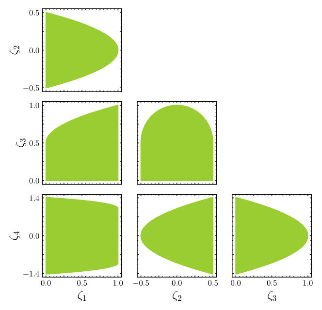
Figure 9: The green region manifests allowed $\zeta$-parameter space onto the projected planes.

and $\Delta_{i}\;(i=0,..,3)$ are given in Appendix B.2. Note that, the parameters $\zeta_{i}\;(i=1,..,4)$ are correlated. The correlation curves in the $\zeta_{i}$ vs. $\zeta_{j}$ planes are given in Appendix C, and their allowed domains are displayed in Figure 9.

4 Unitarity constraints at one-loop

4.1 Partial-wave analysis

In this work, our aim is to study the unitarity bounds on the quartic parameters of Eq. (2.1). Perturbative unitarity constraints come from demanding the unitarity of the $S$-matrix, which reads as,

$$\left|a_{\ell}^{2\to 2}-\frac{1}{2}i\right|^{2}+\mathop{\raisebox{0.0pt}{\scalebox{1.5}{$\displaystyle\sum$}}}_{k>2}\left|a_{\ell}^{2\rightarrow k}\right|^{2}=\frac{1}{4}\,.$$ (4.1)

Here, $a_{\ell}^{2\rightarrow k}$ ’s are the eigenvalues of the $S$-matrix consisting of $\ell$-th partial-wave amplitudes of $2\rightarrow k$ scattering. In the limit, $s\gg|\lambda_{i}\rvert v^{2}$, $s\gg|\mu_{i}\rvert v$, $2\rightarrow 3$ partial-wave amplitudes can be neglected since $\lvert a_{\ell}^{2\rightarrow 3}\rvert^{2}\sim\lambda_{i}^{4}v^{2}/s$, where $\mu_{i}$ ($\lambda_{i}$) ’s represent some linear combinations of scalar cubic (quartic) couplings of the theory. The next leading order contribution comes from $2\rightarrow 4$ scattering amplitudes, which scale as $\lvert a_{\ell}^{2\rightarrow 4}\rvert^{2}\sim\lambda_{i}^{4}$. In the SM, the $2\rightarrow 4$ amplitudes are significantly smaller compared to the $2\rightarrow 2$ partial-wave amplitudes because of the smallness of the quartic coupling PhysRevD.45.3112 . Therefore, in our analysis, only the $2\rightarrow 2$ amplitudes will be taken into account. In the rest of the paper, we remove the superscript $2\to 2$ from partial-wave amplitudes. Under this consideration, Eq. (4.1) gives an upper limit on the eigenvalues of the $S$-matrix,

$$\left|a_{\ell}-\frac{1}{2}i\right|^{2}\,\leq\frac{1}{4}\,.$$ (4.2)

At the tree-level, each of the eigenvalues, $a_{\ell}\in\mathbb{R}$, which leads to a strong bound, $\lvert\text{Re}(a_{\ell})\rvert\,\leq 1/2$. At one-loop and beyond, $a_{\ell}\notin\mathbb{R}$, thus the above stated limit gets weaker when we calculate one-loop and higher order corrections to the $S$-matrix. In the limit, $s\gg\lvert\lambda_{i}\rvert v^{2}\gg M_{W}^{2}$, $s\gg|\mu_{i}|v$ the most dominant contribution comes from the $\ell=0$ partial-wave at tree-level. Therefore, we will only consider $\ell=0$ in our analysis. To calculate the partial-wave amplitude $(a_{0})$ at one-loop level, we adapt the approach of Ref. Grinstein:2015rtl . For a given process $i\to f$, the corresponding matrix element is

$$(a_{0})_{i,f}(s)=\frac{1}{16\pi s}\int_{-s}^{0}dt\mathcal{M}_{i\to f}(s,t)\,,$$

where $\mathcal{M}_{i\rightarrow f}$ represents the sum of all possible scattering amplitudes with an initial state $i$ and final state $f$. As $SU(2)_{L}\otimes U(1)_{Y}$ symmetry is intact at high energies, the $S$-matrix can be sub-divided into smaller block diagonal forms consisting of two-particle states with their respective total charge $(Q)$ and hypercharge $(Y)$. Following this prescription, the basis states are written in Table 2. We have included $1/\sqrt{2}$ symmetry factor in the identical initial or final states. However, this block diagonal structure does not hold beyond the tree-level due to hypercharge interactions. At one-loop level, in general, the off-block diagonal elements are non-zero due to the wavefunction renormalization terms. For a given scattering process with total charge $Q$, if the tree-level blocks have unique eigenvalues, then off-block diagonal elements do not contribute to the tree-level eigenvalues at one-loop, while the contributions can appear at two-loop and beyond. As a first step towards computing unitarity at NLO, we have not considered external wavefunction corrections to the unitarity bounds in the eGM model.

$Q$	$Y$	$2$-particle states
	0	$\phi^{0*}\phi^{0},\frac{\xi^{0}\xi^{0}}{\sqrt{2}},\chi^{0*}\chi^{0},\phi^{+}\phi^{-},\xi^{+}\xi^{-},\chi^{+}\chi^{-},\chi^{++}\chi^{--}$
	1/2	$\phi^{+}\xi^{-},\;\phi^{0}\xi^{0},\;\chi^{+}\phi^{-},\;\phi^{0*}\chi^{0}$
0	1	$\chi^{+}\xi^{-},\;\chi^{0}\xi^{0},\;\frac{\phi^{0}\phi^{0}}{\sqrt{2}}$
	3/2	$\phi^{0}\chi^{0}$
	2	$\frac{\chi^{0}\chi^{0}}{\sqrt{2}}$
	0	$\xi^{+}\xi^{0},\;\chi^{++}\chi^{-},\;\phi^{+}\phi^{0*},\;\chi^{+}\chi^{0*}$
	1/2	$\phi^{0}\xi^{+},\;\phi^{+}\xi^{0},\;\chi^{++}\phi^{-},\;\chi^{+}\phi^{0*}$
1	1	$\phi^{+}\phi^{0},\;\chi^{+}\xi^{0},\;\chi^{++}\xi^{-},\;\chi^{0}\xi^{+}$
	3/2	$\phi^{+}\chi^{0},\;\phi^{0}\chi^{+}$
	2	$\chi^{+}\chi^{0}$
	0	$\chi^{++}\chi^{0*},\;\frac{\xi^{+}\xi^{+}}{\sqrt{2}}$
	1/2	$\phi^{+}\xi^{+},\;\chi^{++}\phi^{0*}$
2	1	$\chi^{++}\xi^{0},\;\chi^{+}\xi^{+},\;\frac{\phi^{+}\phi^{+}}{\sqrt{2}}$
	3/2	$\phi^{+}\chi^{+},\;\phi^{0}\chi^{++}$
	2	$\chi^{++}\chi^{0},\;\frac{\chi^{+}\chi^{+}}{\sqrt{2}}$
	1	$\chi^{++}\xi^{+}$
3	3/2	$\chi^{++}\phi^{+}$
	2	$\chi^{++}\chi^{+}$
4	2	$\frac{\chi^{++}\chi^{++}}{\sqrt{2}}$

Table 2: Initial two-particle states broken down by their total charge $Q$ and total hypercharge $Y$. We have omitted the charge conjugated states as they give the same eigenvalues.

4.2 $2\to 2$ scattering amplitudes

Goldstone-boson equivalence theorem is a useful theoretical tool to study scattering amplitudes in high energy regime Chanowitz:1985hj ; PhysRevD.41.264 ; Lee:1977eg . This theorem states that, at energies, $\sqrt{s}\gg M_{W}$, an amplitude involving $k$ longitudinally polarized vector bosons ($W_{L}^{\pm},Z_{L},h,...$) at the external states can be related to an amplitude with $k$ external Goldstone bosons ($w^{\pm},z,h,...$) as,

$$\mathcal{M}(W_{L}^{\pm},Z_{L},h,...) = (iC)^{k}\mathcal{M}(w^{\pm},z,h,...)\,.$$

In the limit, $s\gg\lvert\lambda_{i}\rvert v^{2}\gg M_{W}^{2}$, $s\gg|\mu_{i}|v$, only one-particle irreducible (1PI) diagrams with two internal lines survive at one-loop. We choose $\overline{\text{MS}}$ scheme to renormalize the quartic couplings in the one-loop computation to satisfy the Goldstone theorem with $C=1$ PhysRevD.41.264 .

The renormalized parameter ($\Lambda$) can be defined in terms of the bare parameter ($\Lambda^{0}$) as,

$$\lambda_{i}^{0}=\lambda_{i}+\delta\lambda_{i}\,,\quad\,\kappa_{i}^{0}=\kappa_{i}+\delta\kappa_{i}\,.$$

Following the convention given in Grinstein:2015rtl , the counter-terms for a given parameter $\Lambda$ can be written as,

$$\delta\Lambda=\frac{1}{16\pi^{2}\epsilon}\beta_{\Lambda}\,,\quad\text{with}\quad\beta_{\Lambda}=16\pi^{2}\mu^{2}\frac{d\Lambda}{d\mu^{2}}\,,$$ (4.3)

where $\mu$ is the renormalization scale. Our one-loop beta functions obtained from Eq. (4.3) are consistent with the existing results in the literature Keeshan:2018ypw ; Blasi:2017xmc ,

$$\beta_{\lambda_{\phi}} =12\lambda_{\phi}^{2}+3\lambda_{\phi\xi}^{2}+\frac{1}{4}\kappa_{2}^{2}+\kappa_{3}^{2}+\frac{3}{2}\lambda_{\phi\chi}^{2}\,,$$

$$\beta_{\lambda_{\xi}} =44\lambda_{\xi}^{2}+\kappa_{1}\lambda_{\chi\xi}+\frac{1}{2}\kappa_{1}^{2}+\frac{3}{2}\lambda_{\chi\xi}^{2}+\lambda_{\phi\xi}^{2}\,,$$

$$\beta_{\lambda_{\chi}} =8\tilde{\lambda}_{\chi}\left(\tilde{\lambda}_{\chi}+\lambda_{\chi}\right)+2\kappa_{1}\lambda_{\chi\xi}+\frac{1}{2}\kappa_{1}^{2}+\frac{1}{4}\kappa_{2}^{2}+14\lambda_{\chi}^{2}+3\lambda_{\chi\xi}^{2}+\lambda_{\phi\chi}^{2}\,,$$

$$\beta_{\tilde{\lambda}_{\chi}} =6\tilde{\lambda}_{\chi}\left(\tilde{\lambda}_{\chi}+2\lambda_{\chi}\right)+\frac{1}{2}\kappa_{1}^{2}-\frac{1}{4}\kappa_{2}^{2}\,,$$

$$\beta_{\kappa_{1}} =\kappa_{1}\left(4\tilde{\lambda}_{\chi}+5\kappa_{1}+8\lambda_{\xi}+2\lambda_{\chi}+8\lambda_{\chi\xi}\right)-\kappa_{3}^{2}\,,$$

$$\beta_{\kappa_{2}} =2\kappa_{2}\left(\lambda_{\chi}-2\tilde{\lambda}_{\chi}+\lambda_{\phi}+2\lambda_{\phi\chi}\right)+2\kappa_{3}^{2}\,,$$

$$\beta_{\kappa_{3}} =\kappa_{3}\Big{(}\kappa_{2}-\kappa_{1}\Big{)}+2\kappa_{3}\Big{(}\lambda_{\chi\xi}+\lambda_{\phi}+2\lambda_{\phi\xi}+\lambda_{\phi\chi}\Big{)}\,,$$

$$\beta_{\lambda_{\phi\xi}} =2\lambda_{\phi\xi}\Big{(}2\lambda_{\phi\xi}+10\lambda_{\xi}+3\lambda_{\phi}\Big{)}+\lambda_{\phi\chi}\Big{(}\kappa_{1}+3\lambda_{\chi\xi}\Big{)}+2\kappa_{3}^{2}\,,$$

$$\beta_{\lambda_{\phi\chi}} =2\lambda_{\phi\chi}\left(\lambda_{\phi\chi}+2\tilde{\lambda}_{\chi}+4\lambda_{\chi}+3\lambda_{\phi}\right)+2\lambda_{\phi\xi}\Big{(}\kappa_{1}+3\lambda_{\chi\xi}\Big{)}+2\kappa_{3}^{2}+\kappa_{2}^{2}\,,$$

$$\beta_{\lambda_{\chi\xi}} =4\lambda_{\chi\xi}\left(\tilde{\lambda}_{\chi}+5\lambda_{\xi}+2\lambda_{\chi}+\lambda_{\chi\xi}\right)+2\kappa_{1}\Big{(}2\lambda_{\xi}+\lambda_{\chi}\Big{)}+\kappa_{1}^{2}+\kappa_{3}^{2}+2\lambda_{\phi\xi}\lambda_{\phi\chi}\,.$$ (4.4)

The complete set of two-loop beta functions for the Yukawa, gauge, and quartic couplings in the theory are given in Appendix E. Up to symmetry factors, one-loop amplitude for a generic 1PI diagram involving four-point vertices is given by,

$$\mathcal{M}_{\textrm{1PI}}^{2\to 2}=\frac{\lambda_{i}\lambda_{j}}{16\pi^{2}}\left[\frac{1}{\epsilon}+2-\ln\left(\frac{-p^{2}-i0_{+}}{\mu^{2}}\right)\right]\,,$$

where the quartic couplings, $\lambda_{i}$ and $\lambda_{j}$ are evaluated at the energy scale, $\mu^{2}=s$. For a given electric charge ($Q$) and hypercharge ($Y$), the $S$-matrix at one-loop can be expressed as,

$$256\pi^{3}\mathbf{a_{0}}=-16\pi^{2}\mathbf{b_{0}}+(i\pi-1)\mathbf{b_{0}}\cdot\mathbf{b_{0}}+3\mathbf{\beta_{b_{0}}}\,,$$ (4.5)

where $\mathbf{b_{0}}$ is the tree-level $S$-matrix and $\mathbf{\beta_{b_{0}}}$ represents the matrix carrying some linear combinations of the beta functions defined in Eq. (4.3). For example, if $b_{0}=a\lambda_{i}+b\lambda_{j}$, then $\beta_{b_{0}}=a\beta_{\lambda_{i}}+b\beta_{\lambda_{j}},\;\forall a,b\in\mathbb{R}$. The comprehensive list of all the scattering matrix elements up to one-loop order are given in Appendix D. For the potential given in Eq. (2.1), we have found 16, 15, 11, 3, 1 unique tree-level eigenvalues for the blocks with $Q=0,1,2,3,4$, respectively. Out of these, total 19 eigenvalues are appeared to be independent, which is in agreement with the results given in the literature Chen:2023ins ,

$$-16\pi a_{0;1} =2\lambda_{\chi\xi}+\kappa_{1}\,,\quad$$

$$-16\pi a_{0;2}^{\pm} =\lambda_{\chi}-2\tilde{\lambda}_{\chi}+\lambda_{\phi}\pm\sqrt{\kappa_{2}^{2}+\left(-\lambda_{\chi}+2\tilde{\lambda}_{\chi}+\lambda_{\phi}\right)^{2}}\,,\quad\quad -16\pi a_{0;3} =\lambda_{\phi\chi}+\frac{\kappa_{2}}{2}\,,$$

$$-16\pi a_{0;4}^{\pm} =4\lambda_{\xi}+\lambda_{\chi}+2\tilde{\lambda}_{\chi}\pm\sqrt{2\kappa_{1}^{2}+\left(-4\lambda_{\xi}+\lambda_{\chi}+2\tilde{\lambda}_{\chi}\right)^{2}}\,,\quad\quad -16\pi a_{0;5} =2\lambda_{\chi\xi}+4\kappa_{1}\,,$$

$$-16\pi a_{0;6}^{\pm} =\lambda_{\phi\xi}+\frac{\lambda_{\phi\chi}}{2}-\frac{\kappa_{2}}{4}\pm\sqrt{\kappa_{3}^{2}+\left(\frac{\kappa_{2}}{4}+\lambda_{\phi\xi}-\frac{\lambda_{\phi\chi}}{2}\right)^{2}}\,,\quad\quad -16\pi a_{0;7} =2\lambda_{\chi}\,,$$

$$-16\pi a_{0;8}^{\pm} =\lambda_{\phi\xi}+\frac{\lambda_{\phi\chi}}{2}+\frac{\kappa_{2}}{2}\pm\sqrt{4\kappa_{3}^{2}+\left(\frac{\kappa_{2}}{2}-\lambda_{\phi\xi}+\frac{\lambda_{\phi\chi}}{2}\right)^{2}}\,,\quad\quad -16\pi a_{0;9} =\lambda_{\phi\chi}-\kappa_{2}\,,$$

$$-16\pi a_{0;10}^{\pm} =\lambda_{\chi\xi}+\lambda_{\phi}-\frac{\kappa_{1}}{2}\pm\sqrt{2\kappa_{3}^{2}+\left(\frac{\kappa_{1}}{2}-\lambda_{\chi\xi}+\lambda_{\phi}\right)^{2}}\,,\quad\quad -16\pi a_{0;11} =2\lambda_{\chi}+6\tilde{\lambda}_{\chi}\,,$$

and $-16\pi a_{0;i}\>(i=12,13,14)$ being the eigenvalues of the following matrix,

$$\begin{bmatrix}20\lambda_{\xi}&2\sqrt{3}\lambda_{\phi\xi}&\sqrt{2}\left(\kappa_{1}+3\lambda_{\chi\xi}\right)\\ 2\sqrt{3}\lambda_{\phi\xi}&6\lambda_{\phi}&\sqrt{6}\lambda_{\phi\chi}\\ \sqrt{2}\left(\kappa_{1}+3\lambda_{\chi\xi}\right)&\sqrt{6}\lambda_{\phi\chi}&8\lambda_{\chi}+4\tilde{\lambda}_{\chi}\\ \end{bmatrix}.$$ (4.6)

5 HEPfit

To constrain the parameters in the GM and eGM model, we employ a Bayesian fit with Markov Chain Monte Carlo (MCMC) simulations. We use the open-source code HEPfit DeBlas:2019ehy to calculate various theoretical and experimental observables that depend on the model parameters and feed them into the parallelized BAT library Caldwell:2008fw . It offers to sample the parameter space and find out allowed regions with all sorts of constraints in a given new physics (NP) model. Approximately, each fit runs over $16$ parallel chains, generating a total of $6.4\times 10^{8}$ iterations.

In our global fits, we consider the lightest $CP$-even scalar to be the SM-like Higgs with fixed mass $m_{h}=125.09$ GeV ATLAS:2015yey , and $v=246.22$ GeV, in the GM and eGM model. All the other SM parameters are fixed to their best fit values deBlas:2016ojx . For the rest of the model parameters, it is important to choose a set of input parameters and their corresponding priors to sample the parameter space in a Bayesian fit. We list the priors of the parameters of GM and eGM model in Table 3 and 4, respectively. The upper limit of triplet vev in our fit is set to be $86$ GeV to avoid any tachyonic mode. In case of eGM model, we make observables for heavy scalar masses within the range: $m_{A},m_{F^{0}},m_{F^{++}}\in[130,1100]$ GeV. We provide the expressions of quartic couplings in terms of physical masses in Appendix A.

Parameter	$v_{\Delta}$	$\alpha$	$\lambda_{3},\lambda_{5}$	$m_{1},m_{3},m_{5}$
Range	$[0,86]$ GeV	$[-\pi/2,\pi/2]$	$[-4\pi,4\pi]$	$[130,1100]$ GeV

Table 3: Priors on the input parameters of GM model.

The Bayesian statistics, in principle, does not provide a unique rule for choosing prior and posterior distributions. It is known that the observables largely depend on the choice of flat priors of the massive parameters Chowdhury:2017aav . However, it is good to choose flat priors for the parameters on which the model observables depend linearly. In order to keep our fit results to be as much prior independent as possible, we choose both flat mass squared priors and flat priors for the other input parameters. Following Chowdhury:2017aav ; Chiang:2018cgb , we use both mass and mass-squared priors in separate global fits and the allowed regions are merged into one. However, we choose only flat mass priors for the NLO unitarity fit in eGM model to reduce computational cost.

Parameter	$v_{\chi}$	$\alpha,\delta$	$\lambda_{\chi}$	$\tilde{\lambda}_{\chi},\kappa_{1},\kappa_{3}$	$m_{H},m_{H^{+}},m_{F^{+}}$
Range	$[0,86]$ GeV	$[-\pi/2,\pi/2]$	$[0,4\pi]$	$[-4\pi,4\pi]$	$[130,1100]$ GeV

Table 4: Priors on the input parameters of eGM model.

Throughout the paper, we will present 99.7% probability regions for fits that include only theoretical constraints, and show the 95.4% CL contours once the Higgs signal strength data are included.

6 Global fit constraints

6.1 Theoretical constraints

From the theory perspective, we include the following constraints in our fits:

• Higgs potential must satisfy the stability bounds between $M_{Z}$ and the scale $\sim 10M_{Z}$.

• Yukawa and quartic couplings of the theory are assumed to be perturbative regime (i.e., their magnitudes are smaller than $\sqrt{4\pi}$ and $4\pi$, respectively) atleast upto the scale $\sim 10M_{Z}$.

• Eigenvalues of the $S$-matrix of $2\to 2$ scattering should satisfy the NLO unitarity bounds. We further demand that the NLO corrections to the LO eigenvalues should be smaller in magnitude. To quantify this, we define the following quantities Grinstein:2015rtl ,

  $$R_{1}=\frac{\mathinner{\!\left\lvert a_{0}^{\text{NLO}}\right\rvert}}{\mathinner{\!\left\lvert a_{0}^{\text{LO}}+a_{0}^{\text{NLO}}\right\rvert}}\,,\qquad R_{1}^{\prime}=\frac{\mathinner{\!\left\lvert a_{0}^{\text{NLO}}\right\rvert}}{\mathinner{\!\left\lvert a_{0}^{\text{LO}}\right\rvert}}\,,$$ (6.1)

  where $a_{0}^{\textrm{NLO}}$ stands for NLO corrections calculated in the eigenbasis of the matrix, $\mathbf{a}_{0}^{\textrm{LO}}$.

Therefore, the perturbative expansion is not valid at NLO when $R_{1}^{\prime}=1$ or $R_{1}=1$. Similar criteria were used in case of the SM PhysRevD.45.3112 and later in 2HDM Grinstein:2015rtl ; Cacchio:2016qyh to analyze perturbative unitarity. However, there are certain directions in the parameter space that lead to accidental cancellations in the LO amplitudes. For example, $a_{0}^{\textrm{LO}}=\kappa_{2}-\lambda_{\phi\chi}$ is small when $\kappa_{2}\approx\lambda_{\phi\chi}$, while the NLO correction can be large since it depends on other quartic couplings of the theory (see Eq. (4.6)). Therefore, while doing $R_{1}^{\prime}$ test, we impose a cut on the tree-level eigenvalues, $|a_{0}^{\textrm{LO}}|>0.02$ (or, equivalently, $|\lambda_{i}|,|\kappa_{i}|>1/2$), such that the fit does not encounter any such accidental cancellations for reasonable values of the quartic couplings. Furthermore, it is worth noting that the bounds on the eigenvalues of the $S$-matrix are obtained at very high energy, $s\gg\lvert\lambda_{i}\rvert v^{2}\gg M_{W}^{2}$, $s\gg|\mu_{i}|v$. However, the running of the VEVs destabilize the custodial symmetric vacua Blasi:2017xmc . Therefore, the constraints on the model parameters (see Eqs. (2.5) and (2.6)) no longer hold in the high energy limit. In order to make it consistent with the $S$-matrix computations, we consider the most general potential (Eq. (2.1)) containing ten quartic couplings and we use the one-loop unitarity conditions on these couplings. Our results of the $S$-matrix elements at one-loop are given in Appendix D. For the renormalization group runnings, we use two-loop RGEs, which are computed using PyR@TE Sartore:2020gou . Explicit expressions of two-loop RGEs are given in Appendix E. Among the Yukawa’s we only consider the contributions coming from third generation fermions.

	Signal	Value	Correlation matrix						${\cal L}$	Source
	strength								[fb-1]
	$\mu_{\text{ggF,bbh}}^{\gamma\gamma}$	$1.04\pm 0.10$	1	$-0.13$	0	0	0	0		ATLAS:2022tnm
	$\mu_{\text{VBF}}^{\gamma\gamma}$	$1.20\pm 0.26$	$-0.13$	1	0	0	0	0
	$\mu_{\text{Wh}}^{\gamma\gamma}$	$1.5\pm 0.55$	0	0	1	$-0.37$	0	$-0.11$
	$\mu_{\text{Zh}}^{\gamma\gamma}$	$-0.2\pm 0.55$	0	0	$-0.37$	1	0	0
	$\mu_{\text{tth}}^{\gamma\gamma}$	$0.89\pm 0.31$	0	0	0	0	1	$-0.44$	139 d
	$\mu_{\text{th}}^{\gamma\gamma}$	$3\pm 3.5$	0	0	$-0.11$	0	$-0.44$	1
	$\mu_{\text{ggF}}^{ZZ}$	$0.95\pm 0.1$	1	$-0.22$	$-0.27$	0				ATLAS:2020rej
	$\mu_{\text{VBF}}^{ZZ}$	$1.19\pm 0.45$	$-0.22$	1	0	0
	$\mu_{\text{Vh}}^{ZZ}$	$1.43\pm 1.0$	$-0.27$	0	1	$-0.18$			139 d
	$\mu_{\text{tth}}^{ZZ}$	$1.69\pm 1.45$	0	0	$-0.18$	1
	$\mu_{\text{incl.}}^{ZZ}$	$1.0\pm 0.1$							139	ATLAS:2020rej
	$\mu_{\text{ggF,bbh}}^{WW}$	$1.15\pm 0.135$
	$\mu_{\text{VBF}}^{WW}$	$0.93\pm 0.21$							139	ATLAS:2022ooq
	$\mu_{\text{ggF,bbh,VBF}}^{WW}$	$1.09\pm 0.11$
	$\mu_{\text{VBF}}^{\tau\tau}$	$0.90\pm 0.18$	1	$-0.24$	0	0				ATLAS:2022yrq
	$\mu_{\text{ggF,bbh}}^{\tau\tau}$	$0.96\pm 0.31$	$-0.24$	1	$-0.29$	0
	$\mu_{\text{Vh}}^{\tau\tau}$	$0.98\pm 0.60$	0	$-0.29$	1	0			139
	$\mu_{\text{tth,th}}^{\tau\tau}$	$1.06\pm 1.18$	0	0	0	1
	$\mu_{\text{VBF}}^{bb}$	$0.95\pm 0.37$							126	ATLAS:2020bhl
	$\mu_{\text{Wh}}^{bb}$	$0.95\pm 0.26$							139	ATLAS:2020fcp
	$\mu_{\text{Zh}}^{bb}$	$1.08\pm 0.24$							139	ATLAS:2020fcp
	$\mu_{\text{Vh}}^{bb}$	$1.02\pm 0.17$							139	ATLAS:2020fcp
	$\mu_{\text{tth,th}}^{bb}$	$0.35\pm 0.35$							139	ATLAS:2021qou
	$\mu_{\text{pp}}^{\mu\mu}$	$1.2\pm 0.6$							139	ATLAS:2020fzp
	$\mu_{\text{pp}}^{Z\gamma}$	$2.0\pm 0.95$							139	ATLAS:2020qcv

Table 5: Latest Run 2 data on $h$ signal strengths measured by ATLAS at $\sqrt{s}=13$ TeV. Correlations below $0.1$ are treated to be zero. The colors in the first column represent the corresponding decay channels in Figure 5.

6.2 $h$ signal strengths

For a given process of producing SM-like Higgs $h$ with an initial state $i$ and decay to final state $f$, the signal strength for the production ($\mu_{i}$) and for the decay ($\mu_{f}$) are given by,

$$\mu_{i}=\frac{\sigma_{i}}{(\sigma_{i})_{\textrm{SM}}}\,,\quad\textrm{and}\quad\mu_{f}=\frac{\mathcal{B}(h\to f)}{\mathcal{B}_{\textrm{SM}}(h\to f)}\,,$$

where $\sigma_{i}$’s are the production cross sections for $i\in\{gg$F$,\,bbh,\,$VBF$,\,Wh,\,Zh,\,tth,\,th\}$, and $\mathcal{B}(h\to f)$’s are the decay branching fractions for $f\in\{ZZ,\,WW,\,\gamma\gamma,\,Z\gamma,\,\mu\mu,\,bb,\,\tau\tau\}$. Signal strength for the combined process with production channel ($i$) and the decay mode ($f$) of $h$ can be defined as,

$$\mu_{i}^{f}\equiv\mu_{i}\cdot\mu_{f}=r_{i}\cdot\frac{r_{f}}{\sum_{f^{\prime}}r_{f^{\prime}}\cdot\mathcal{B}_{\textrm{SM}}(h\to f^{\prime})}\,,$$

where $r_{i}$ and $r_{f}$ are the ratios of the $\sigma_{i}$’s and the total decay width $\Gamma^{f}$’s with respect to their corresponding SM values.

	Signal	Value	Correlation matrix				${\cal L}$	Source
	strength						[fb-1]
	$\mu_{\text{ggh,bbh}}^{\gamma\gamma}$	$1.07\pm 0.11$						CMS:2021kom
	$\mu_{\text{VBF}}^{\gamma\gamma}$	$1.04\pm 0.32$
	$\mu_{\text{Vh}}^{\gamma\gamma}$	$1.34\pm 0.34$					137 d
	$\mu_{\text{tth,th}}^{\gamma\gamma}$	$1.35\pm 0.31$
	$\mu_{\text{ggh,bbh,tth,th}}^{ZZ}$	$0.95\pm 0.13$	1	$-0.11$				CMS:2021ugl
	$\mu_{\text{VBF,Vh}}^{ZZ}$	$0.82\pm 0.34$	$-0.11$	1			137 d
	$\mu_{\text{ggh}}^{WW}$	$0.92\pm 0.11$	1	$-0.13$	0	0		CMS:2022uhn
	$\mu_{\text{VBF}}^{WW}$	$0.71\pm 0.26$	$-0.13$	1	0	0
	$\mu_{\text{Zh}}^{WW}$	$2.0\pm 0.7$	0	0	1	0
	$\mu_{\text{Wh}}^{WW}$	$2.2\pm 0.6$	0	0	0	1	138 d
	$\mu_{\text{incl.}}^{\tau\tau}$	$0.93\pm 0.12$						CMS:2022kdi
	$\mu_{\text{ggh}}^{\tau\tau}$	$0.97\pm 0.19$
	$\mu_{\text{qqh}}^{\tau\tau}$	$0.68\pm 0.23$
	$\mu_{\text{Vh}}^{\tau\tau}$	$1.80\pm 0.44$					138 d
	$\mu_{\text{qqh}}^{bb}$	$1.59\pm 0.60$	1	$-0.75$				CMS:2023tfj
	$\mu_{\text{ggh}}^{bb}$	$-2.7\pm 3.89$	$-0.75$	1			90.8 d
	$\mu_{\text{ggh,tth}}^{\mu\mu}$	$0.66\pm 0.67$	1	$-0.24$				CMS:2020xwi
	$\mu_{\text{VBF,Vh}}^{\mu\mu}$	$1.85\pm 0.86$	$-0.24$	1			137
	$\mu_{\text{pp}}^{Z\gamma}$	$2.4\pm 0.9$					138	CMS:2022ahq

Table 6: Latest Run 2 data on $h$ signal strengths measured by CMS at $\sqrt{s}=13$ TeV. Correlations below $0.1$ are treated to be zero. The colors in the first column represents the corresponding decay channels in Figure 5.

Therefore, the signal strength for a particular decay mode implicitly depends on all the other $h$-decay modes. In the $\kappa$-framework ATLAS:2016neq , the modifiers for SM $h$ coupling to vector bosons and fermions at tree-level in both GM and eGM model are given by,

$$\kappa_{V}=c_{\alpha}c_{\beta}-\sqrt{\frac{8}{3}}s_{\alpha}s_{\beta}\,,\quad\textrm{and}\quad\kappa_{f}=\frac{c_{\alpha}}{c_{\beta}}\,,$$ (6.2)

At leading order (LO), the $h$ decays into $\gamma\gamma$ and $Z\gamma$ channels are mediated via exotic charged Higgs bosons ($F^{++},F^{+},H^{+}$) at one-loop. Due to the non-degenerate masses in the CS multiplets in eGM model, both singly- and doubly-charged heavy Higgs bosons contribute separately to the above loop mediated decay modes. The general expressions of $r_{\gamma\gamma}$ and $r_{Z\gamma}$ involving SM constituents and exotic charged particles are given in Gunion:1989we . The experimental input values of $h$ signal strengths from the latest ATLAS and CMS Run 2 data at a centre-of-mass energy of $13$ TeV are displayed in Table 5 and 6, respectively. ATLAS and CMS combination for Run 1 data on $h$ signal strengths measurements are given in Table 2 of Chowdhury:2017aav .

7 Results

In this section, we present the results of the fits to theoretical and Higgs signal strength constraints for both GM and eGM model. In Figure 1, we display the 99.7% confidence level (CL) allowed regions in the $\lambda_{2}$ vs. $\lambda_{3}$ ($\lambda_{\xi}$ vs. $\lambda_{\chi}$) plane with three different bounded from below (BFB) conditions for GM (eGM) model. The grey (yellow) region manifests allowed parameter space that satisfies the BFB conditions with all possible combinations of any two (three) non-vanishing field directions. The green area shows the allowed parameter space if we impose the BFB conditions considering all the 13-fields having non-vanishing values.

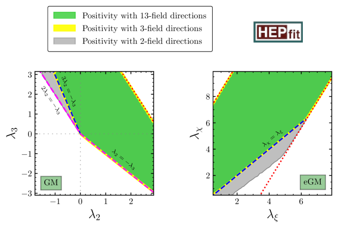
Figure 1: Comparison of different BFB conditions in the $\lambda_{2}$ vs. $\lambda_{3}$ plane (left) of the GM model and $\lambda_{\xi}$ vs. $\lambda_{\chi}$ plane (right) of the eGM model. The grey, yellow, and green areas are allowed if we use the BFB conditions with all possible two, three and thirteen non-vanishing field directions at once, respectively. The red dotted lines at the boundary imply perturbativity bounds. The blue dashed boundary lines are originated from the BFB conditions with all possible three non-vanishing field directions at once. The BFB conditions that restrict the couplings to have negative values in the right panel, disallow the region to the left side of the magenta dashed lines in the left panel.

Let us try to explain the boundaries of the allowed regions. The red dotted lines are anticipated from the perturbativity bounds of the quartic couplings, $|\lambda_{i}|,\;|\kappa_{i}|\leq 4\pi$. The magenta dashed lines in the left panel of Figure 1 reflect the necessary and sufficient BFB conditions for eGM model, $\lambda_{\chi}>0$ and $\lambda_{\xi}>0$, that lead to $2\lambda_{2}>-\lambda_{3}$ and $\lambda_{2}>-\lambda_{3}$ in the GM limit. Blue dashed lines represent the limiting curves coming from one of the necessary and sufficient conditions with three and all non-vanishing field directions, $\lambda_{\chi}>\lambda_{\xi}$ ($3\lambda_{2}>-\lambda_{3}$ for GM model). It is worth to note that these BFB conditions are imposed to the tree-level potential and the quartic couplings ($\lambda_{i},\kappa_{i}$) are interpreted at the scale of $M_{Z}$. From Figure 1, one can see that BFB conditions with all possible 3-field directions and 13-field directions generate a large overlapping parameter space. Therefore, in the rest of our analysis, we shall consider the BFB conditions with all possible 3-field directions only to reduce computational cost. Effects of these different BFB conditions in the rest of the quartic coupling planes in the eGM model are given in Appendix F.

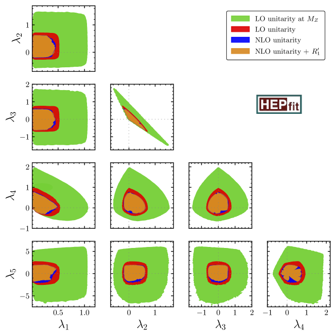
Figure 2: Allowed regions in the $\lambda_{i}$ vs. $\lambda_{j}$ planes of the GM model with a 99.7% probability. The red (blue) colored areas show the allowed parameter space if we use LO (NLO) unitarity bounds without violating the stability of the potential. The brown region are obtained with the additional condition that the NLO value should be smaller than LO value in magnitude (if the LO value is not accidentally small), and the green area are allowed if we impose the unitarity conditions at the scale $M_{Z}$. All the $\lambda_{i}$ values are given at $M_{Z}$ scale.

Next, we compare different unitarity constraints on the parameter spaces for both GM and eGM model. In Figure 2 (Figure 3), we show the 99.7% CL allowed regions, at $M_{Z}$ scale, in the quartic coupling planes of GM (eGM) model with LO, NLO unitarity, and NLO unitarity with $R_{1}^{\prime}$ (see Eq. (6.1)) in the colors, red, blue, and brown, respectively. It is distinctly evident from Figures 2 and 3 that the NLO unitarity constraint sets substantially stringent bounds on the parameter space compared to the LO unitarity. The allowed region gets further compressed when we include the perturbativity condition ($R_{1}^{\prime}<1$) in addition to the NLO unitary bounds. Interplay between unitarity and perturbativity conditions places stronger bounds on certain directions of the quartic coupling planes (see e.g., $\lambda_{4}$ vs. $\lambda_{5}$ plane in GM and $\kappa_{3}$ vs. $\lambda_{\phi\xi}$ plane in eGM model). A detailed discussion on the features that exhibit sharp cuts towards the origins of the planes are given in Appendix F. If we use LO unitarity conditions at $M_{Z}$ scale instead, the parameter space gets much more relaxed. These regions are shown in green color in the same planes of Figures 2 and 3. Numerically, the quartic couplings for the GM (eGM) model can have maximum absolute value as large as 3.0, 2.2, or 2.0 (9.0, 5.2, or 5.0), if we apply LO, NLO, or $R_{1}^{\prime}$-perturbative NLO unitarity, respectively. These values are obtained from the Figures 2 and 3.

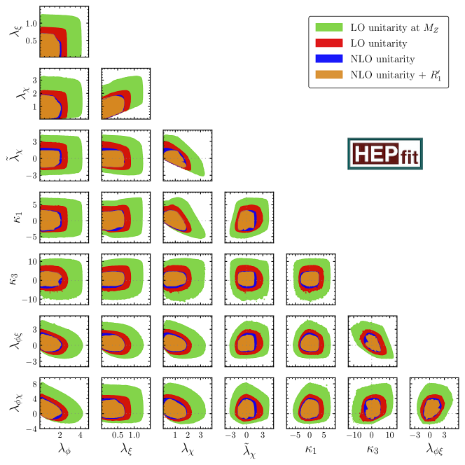
Figure 3: 99.7% CL allowed regions in the quartic coupling planes of the eGM model. The colors of the shaded regions have the same meaning here as in Figure 2.

An in-depth study of different unitarity conditions for the GM model are displayed on $\lambda_{3}$ vs. $\lambda_{4}$ plane in the right panel of Figure 4. The red, blue, and brown solid lines correspond to the contours of the same color as in Figure 2. The red dashed contour is the result of imposing LO unitarity with LO RGEs and it is almost always more stringent than the choice of LO unitarity with NLO RGEs. This is due to the fact that LO RGEs run the quartic couplings into non-perturbative values at much lower energy scale in comparison with NLO RGE running. Therefore, larger values of quartic couplings are allowed at $M_{Z}$ scale if one uses NLO RGE. The violet contour represents the allowed region while we demand $R_{1}^{\prime}$-perturbative LO unitarity and the contour shows some distinct pinch-cuts. A weaker bound comes from Eq. (4.2) where we put 1/2 as upper limit for the absolute value of real-part of the NLO unitarity eigenvalues. This contour is represented by blue dotted line and it is always less stringent than the blue solid contour. Finally, the cyan contour corresponds to the allowed regions satisfying $R_{1}$-perturbative (see Eq. (6.1)) unitarity condition and the contour is almost overlapping with the brown one. The left panel in Figure 4 shows how the constraints on the quartic couplings translate into the mass difference planes of the heavy Higgs bosons in the GM model. The different unitarity constraints follow the same ordering as in the right panel. While LO unitarity allows for maximum $\mathinner{\!\left\lvert m_{3}-m_{1}\right\rvert}\sim 500$ GeV and $\mathinner{\!\left\lvert m_{5}-m_{3}\right\rvert}\sim 800$ GeV, perturbative NLO unitarity conditions set a stringent upper limit of $\sim 300$ GeV and $\sim 700$ GeV for this absolute mass differences, respectively.

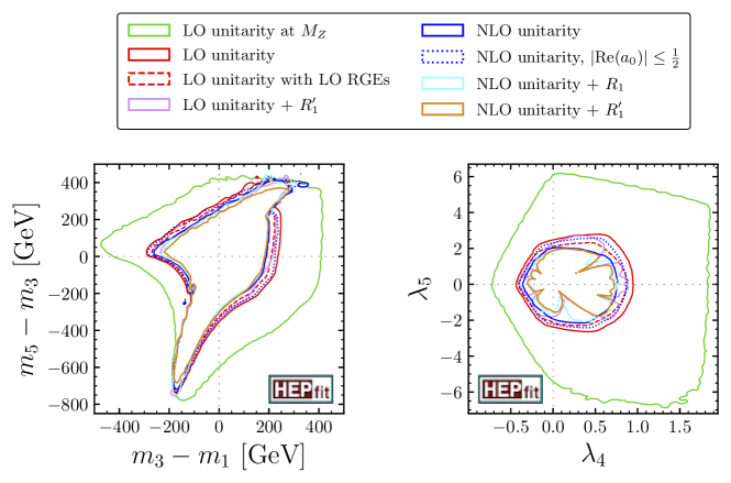
Figure 4: Comparison of the effects of different unitarity constraints in the $m_{3}-m_{1}$ vs. $m_{5}-m_{3}$ plane (left) and $\lambda_{4}$ vs. $\lambda_{5}$ plane (right) of GM model. The green, red, blue, and brown contours have the same meaning as in Figure 2. The red dashed contour shows the effects of LO RGEs to the LO unitarity conditions, and the pink contour demonstrates the impact of $R_{1}^{\prime}$-perturbative condition without imposing NLO unitarity bounds. The dotted blue contour shows the allowed regions if we consider only real-parts of the $S$-matrix eigenvalues while imposing unitarity bounds at one-loop, and the cyan contour represents the allowed area if we include $R_{1}$-perturbative condition with NLO unitarity bounds.

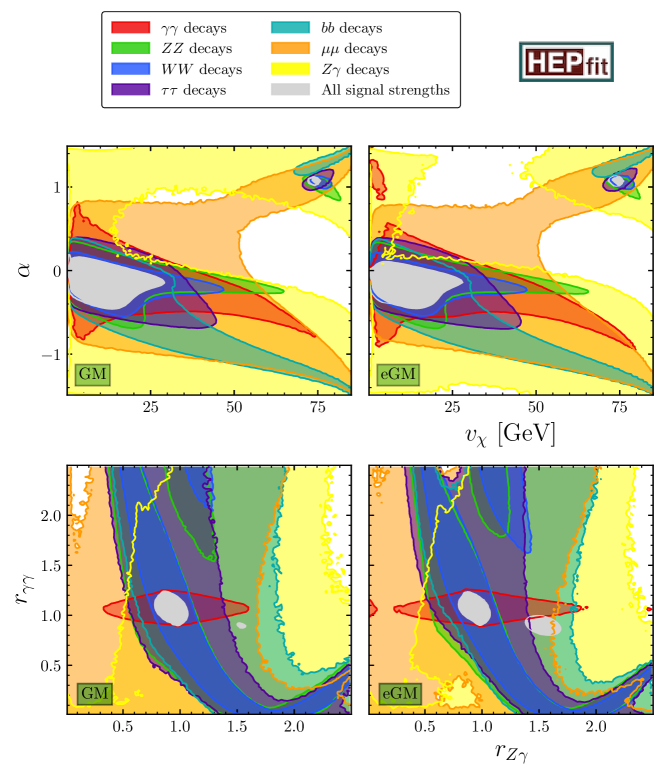
Figure 5: 95.4% probability regions show the impact of the Higgs signal strengths for different final states in the $v_{\chi}$ vs. $\alpha$ planes (top) and the relative one-loop Higgs couplings planes (bottom). The individual fits to full Run 1 and Run 2 data from $h$ decays to $\gamma\gamma,\,ZZ,\,WW,\,\tau\tau\,,\,bb,\,\mu\mu\,,$ and $Z\gamma$ in red, green, blue, purple, cyan, orange, and yellow, respectively. The results from the combined fits is shown in the grey color shaded regions.

In the top left (top right) panel of Figure 5, we display the impacts of the individual signal strengths with different final states on the $v_{\chi}$ vs. $\alpha$ plane for the GM (eGM) model. For small $v_{\chi}$ and the region where $\alpha$ is not close to zero, the $ZZ$ and $WW$ signal strengths are most restrictive. Whereas, for large $v_{\chi}$ values, the most significant constraint around $\alpha=0$ region, comes from $h\rightarrow b\bar{b}$ data. The combined fit with all signal strengths exhibits allowed range of $\alpha$ to be $-0.25<\alpha<0.2$ at a $95.4\%$ confidence level and the triplet VEV $v_{\chi}$ cannot exceed $30$ GeV for both GM and eGM model. In the decoupling limit, $\alpha,v_{\chi}\to 0$ Hartling:2014zca , all additional Higgs bosons become heavy and the couplings of the SM-like Higgs approach towards its SM values, which translate into $\kappa_{V}=1$ (see Eq. (6.2)). Away from the decoupling limit, $\kappa_{V}$ is no longer unity at tree-level. In the combined fit, we find that the Higgs signal strength data disfavor the region where $\kappa_{V}>1.05$ with a $95.4\%$ CL. Additionally, we find a tiny allowed region around $(\alpha,v_{\chi})=(1,75)$. This features a negative-sign for the $h$ couplings to vector bosons relative to their SM values, i.e., $\kappa_{V}<0$ in this region. Amongst the loop mediated decays, $h\to\gamma\gamma$ channel stringently constrain $v_{\chi}$ vs. $\alpha$ plane compared to $h\to Z\gamma$ channel. In bottom left (right) panel of Figure 5, we show the allowed ranges in $r_{Z\gamma}$ vs. $r_{\gamma\gamma}$ plane for all different final states for GM (eGM) model. The dominant allowed region from the combined fit stays around the SM values. The maximal deviation of $r_{\gamma\gamma}$ and $r_{Z\gamma}$ from their SM values are roughly $25\%$ and $20\%$ in GM (eGM) model, respectively. However, here also small disconnected allowed regions have been observed in consistence with the $v_{\chi}$ vs. $\alpha$ plane.

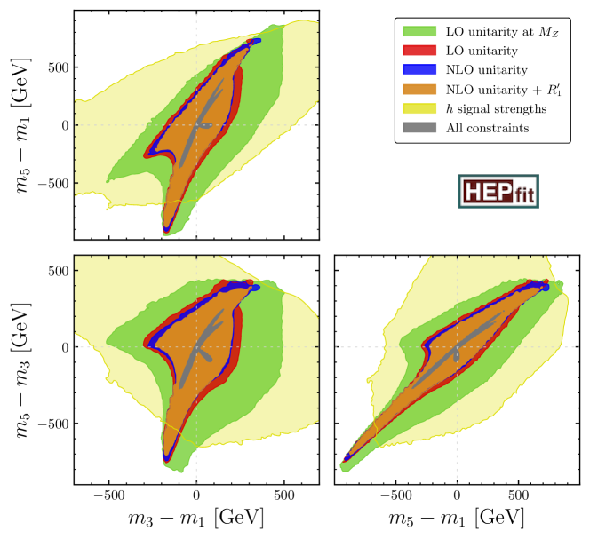
Figure 6: Allowed regions in the mass difference planes in the GM model. The green, red, blue, and brown area have the same meaning as the regions of same color in Figure 2. The yellow regions are allowed from the Higgs signal strengths measurements with a $95.4\%$ CL. Finally, the grey areas are allowed from the combined fits to the theory and Higgs signal strengths constraints.

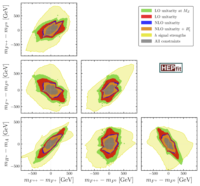
Figure 7: Effects of different constraints in the planes of heavy Higgs boson mass difference within the member of each CS multiplets in eGM model. The shaded regions are allowed and the colors have the same meaning as in Figure 6.

In Figure 6, we present the effects of different theoretical constraints and the latest Higgs signal strength data on the mass differences of heavy Higgs bosons in the GM model. The green, red, blue, and brown area correspond to the same regions as in Figure 2. The yellow shaded area shows the allowed region from the Higgs signal strength data at a 95.4% CL. The grey area is the 95.4% CL allowed region after all the theoretical and Higgs signal strength constraints are taken into consideration. The combined fit allows for a maximal mass splitting between $m_{1}$, $m_{3}$, and $m_{5}$ is of around 400 GeV in GM model. Note that, the largest possible absolute value of these mass differences is reduced by about $100$ GeV than that is allowed from the fit in Ref. (Chiang:2018cgb, ). This is due to the combined effect of state-of-the-art stability and NLO unitarity bounds. Among these mass differences, one can see that $m_{3}-m_{1}$ is strongly constrained from the theoretical constraints and cannot exceed 150 GeV in magnitude. In Figure 6, after marginalizing over all other parameters, the viable regions away from the diagonal, around $m_{3}-m_{1}=50$ GeV and $m_{5}-m_{3}=-50$ GeV ($m_{5}-m_{1}=0$), are a consequence of $k_{V}<0$ and can be ruled out from direct searches. On the other hand, Figure 7 shows the effect of all these constraints on the mass splittings within the members of each CS multiplet in eGM model. The heavy Higgs with mass difference greater than 380 GeV is excluded at $95\%$ CL and the intra-multiplet mass difference can maximally reach 210 GeV in the eGM model. It is distinct from these plots that the theory bounds play a dominant role over the Higgs signal strength in constraining the allowed mass differences of exotic heavy Higgs bosons.

Finally, Figure 8 shows the allowed 95.4% probability limits of the quartic couplings and heavy Higgs mass differences if we combine all the constraints. We observed that the mass difference of $m_{F^{++}}$ and $m_{F^{0}}$ is more robust compared to the other mass differences in our global fit, and the difference cannot exceed $210$ GeV in magnitude. For details, we refer to Eq. (2.9) in Section 2. The maximal mass splitting is $\sim 400$ GeV for all heavy Higgs masses above 700 GeV in the GM model, and this further reduces to $\sim 130$ GeV in the eGM model.

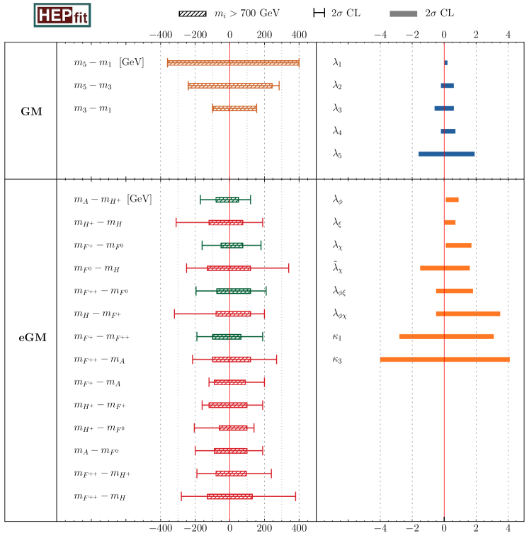
Figure 8: Allowed mass differences of the heavy Higgs bosons and quartic couplings from the global fit in both GM and eGM model. The horizontal bars (bands) denote the 95.4% confidence interval. The hatched area indicates the allowed intervals if the masses of the heavy Higgs bosons are greater than $700$ GeV. The allowed ranges for physical masses are obtained from the Figures 12 and 13.

8 Conclusions

A minimal triplet scalar extension of the SM, that preserves $\rho=1$ at tree-level, results in the eGM model. Unlike the GM model, this model offers mass non-degenerate CS multiplets in the scalar sector and therefore naturally has richer phenomenological aspects. For the GM and eGM models, we have presented global fits to the NLO unitary bounds, stability constraints, and recent $h$ signal strength data from the LHC. In order to systematically improve the state-of-the-art theoretical bounds, we have extracted the necessary and sufficient conditions for the stability bounds on the most general GM potential considering all possible combinations of field directions. We have computed one-loop corrections to the tree-level eigenvalues of $S$-matrix for all $2\to 2$ bosonic scatterings, and placed unitarity bounds on the two-loop renormalization group improved quartic couplings in the most general GM potential. From the fit, we have observed that the stability (BFB) conditions considering all 13-field directions render more parameter space, having large quartic coupling values, accessible that were unavailable if we impose stability conditions with 3-field directions only (see Figure 10). However, at small quartic coupling values, imposing stability (BFB) conditions with 3-field and all 13-field directions generate a large overlapping parameter space. Since we have seen that the NLO unitarity conditions disallow large quartic coupling values (see Figures 2 and 3), it is justified to appoint stability conditions with 3-filed directions only in our fits. We have found that the allowed parameter space of both GM and eGM model get more constrained once we go from LO to NLO unitarity conditions. Imposing perturbativity condition with NLO unitarity further reduces the allowed parameter space. Considering all theoretical constraints in the fit, we have observed that the 99.7% CL allowed values of the quartic couplings cannot exceed 2.0 (5.0) in magnitude and found that the mass difference between any two heavy Higgs masses cannot be larger than $850$ GeV ($400$ GeV) in the GM (eGM) model.

In detail, we have showed the impacts of the individual Higgs signal strengths on leading order $h$ couplings using the Run 1 and latest Run 2 data from the CMS and ATLAS detector. By considering all available Higgs signal strength data, we find that the triplet VEV, $v_{\chi}$, and mixing angle, $|\alpha|,$ cannot exceed 30 GeV and 0.25, respectively (or, equivalently $k_{V}\not>1.05$) at a 95.4% CL in both GM and eGM model. At one-loop, the couplings of $h$ to $\gamma\gamma$ ($Z\gamma$) cannot differ by more than $25\%$ ($20\%$) from its SM value. In our fits, marginalizing over all other parameters, we found a viable region around $v_{\chi}=75$ GeV and $\alpha=1$, featuring a negative sign for $h$ coupling to the vector bosons. This region can be probed once the direct search results at low-masses ($m_{i}<200$ GeV) get improved (Chiang:2018cgb, ).

Combining all theoretical constraints and the latest $h$ signal strength data, we find the following ranges of the model parameters, with a $95.4\%$ CL, while marginalizing over all other parameters: The mass differences between the heavy Higgs bosons cannot exceed 400 GeV ($380$ GeV) in the GM (eGM) model. In case of eGM model, the above stated limit further reduce to $\mathcal{O}(100)$ GeV when the masses of all heavy Higgs bosons are above 700 GeV. The maximal mass splitting between the members of each CS multiplets cannot be larger than 210 GeV in the eGM model. Interestingly, one such mass difference between the doubly-charged Higgs ($F^{++}$) and $CP$-even Higgs ($F^{0}$) does not depend on the model parameters, $\mu_{1}$ and $\mu_{2}$ (see Eq. (2.9)), which makes this result more robust compared to the other mass differences. This opens up the possibility to study novel signatures that could potentially be observed at the LHC and other future colliders.

Appendix A Quartic couplings from physical masses

In this appendix we provide the expressions of quartic couplings ($\lambda_{i},\kappa_{i}$) in terms of physical masses for the eGM model.

$$\lambda_{\phi} =\frac{1}{2v^{2}c_{\beta}^{2}}\Big{(}m_{h}^{2}c_{\alpha}^{2}+m_{H}^{2}s_{\alpha}^{2}\Big{)},$$

$$\lambda_{\xi} =\frac{1}{3v^{2}s_{\beta}^{2}}\Big{(}m_{h}^{2}s_{\alpha}^{2}+m_{H}^{2}c_{\alpha}^{2}+2m_{F^{0}}^{2}+3\Big{(}M_{2}^{2}-2m_{A}^{2}\Big{)}c_{\beta}^{2}-\frac{3}{2}M_{1}^{2}\Big{)},$$

$$\lambda_{\chi} =\frac{2}{3v^{2}s_{\beta}^{2}}\Big{(}2m_{h}^{2}s_{\alpha}^{2}+2m_{H}^{2}c_{\alpha}^{2}+m_{F^{0}}^{2}-3m_{A}^{2}c_{\beta}^{2}\Big{)},$$

$$\lambda_{\phi\xi} =\frac{1}{v^{2}s_{\beta}c_{\beta}}\Big{(}s_{\beta}c_{\beta}\Big{(}2m_{A}^{2}-M_{2}^{2}\Big{)}+\sqrt{\frac{2}{3}}\Big{(}M_{H}^{2}-m_{h}^{2}\Big{)}c_{\alpha}s_{\alpha}\Big{)},$$

$$\tilde{\lambda}_{\chi} =\frac{2}{v^{2}s_{\beta}^{2}(c_{\delta}-c_{\beta}s_{\delta})}\left[c_{\delta}\Big{(}m_{F^{++}}^{2}-M_{1}^{2}+\Big{(}2M_{2}^{2}+m_{A}^{2}-4m_{H^{+}}^{2}\Big{)}c_{\beta}^{2}\Big{)}\right.$$

$$\quad\qquad\qquad\qquad\qquad\left.+c_{\beta}s_{\delta}\Big{(}-m_{F^{++}}^{2}+M_{1}^{2}+\Big{(}3m_{A}^{2}-2M_{2}^{2}\Big{)}c_{\beta}^{2}\Big{)}\right],$$

$$\kappa_{1} =\frac{4}{v^{2}s_{\beta}^{2}(c_{2\delta}-c_{\beta}s_{2\delta})}\left[-M_{1}^{2}c_{2\delta}+\Big{(}c_{\delta}^{2}m_{F^{+}}^{2}-s_{\delta}^{2}m_{H^{+}}^{2}\Big{)}s_{\beta}^{2}+2\Big{(}M_{2}^{2}-m_{A}^{2}\Big{)}c_{\beta}^{2}c_{2\delta}\Big{)}\right.$$

$$\qquad\left.+\Big{(}m_{F^{+}}^{2}-m_{H^{+}}^{2}\Big{)}c_{\beta}^{2}+c_{\beta}s_{2\delta}\Big{(}M_{1}^{2}+m_{A}^{2}-m_{F^{+}}^{2}-m_{H^{+}}^{2}-\Big{(}2M_{2}^{2}-3m_{A}^{2}\Big{)}c_{\beta}^{2}\Big{)}\right],$$

$$\kappa_{2} =\frac{4}{v^{2}(c_{2\delta}-c_{\beta}s_{2\delta})}\Big{(}2s_{\delta}^{2}m_{F^{+}}^{2}-2c_{\delta}^{2}m_{H^{+}}^{2}+\Big{(}M_{2}^{2}+m_{A}^{2}\Big{)}c_{2\delta}-\Big{(}M_{2}^{2}-m_{A}^{2}\Big{)}c_{\beta}s_{2\delta}\Big{)},$$

$$\kappa_{3} =\frac{2\sqrt{2}}{v^{2}}\Big{(}M_{2}^{2}-m_{A}^{2}\Big{)},$$ (A.1)

where we have defined,

$$M_{1}^{2}=\frac{\mu_{1}s_{\beta}v}{\sqrt{2}}\,,\quad M_{2}^{2}=\frac{\mu_{2}v}{\sqrt{2}s_{\beta}}\,.$$ (A.2)

These eight quartic couplings can be reduced to five $\lambda_{i}\,(i=1,2,3,4,5)$ , in the limit $\delta=0,\;m_{A}=m_{H^{+}},$ and $m_{F^{0}}=m_{F^{+}}=m_{F^{++}}$ (also known as the GM limit), which are consistent with the relations given in Chiang:2012cn . The relations between the quartic couplings in the GM and eGM models are given in Table 1.

Appendix B Positivity criteria in the field subspace

Here we consider the subspaces of the potential where only two or three fields are non-vanishing at once. At large field values, only quartic terms in the potential dominate as in Eq. (3.1).

B.1 2-field directions

In the absence of any coupling between doublet and triplet scalars, we consider a field direction where only electrically neutral components $(\chi^{0},\xi^{0})$ are non-vanishing. The corresponding potential reads,

$$V_{2.0}^{(4)}=\lambda_{\chi}|\chi^{0}|^{4}+\lambda_{\chi\xi}|\chi^{0}|^{2}(\xi^{0})^{2}+\lambda_{\xi}(\xi^{0})^{4}\,.$$ (B.1)

Due to the bi-quadratic form of the potential in Eq. (B.1), the necessary and sufficient BFB conditions are nothing but the criteria for strict copositivity of the potential, given by,

$$\lambda_{\chi}>0\;\land\;\lambda_{\xi}>0\;\land\;\lambda_{\chi\xi}+2\sqrt{\lambda_{\chi}\lambda_{\xi}}>0\,.$$ (B.2)

Similarly, the potential for all possible field directions with only two non-vanishing fields at once are listed below,

$$V^{(4)}_{2.1} =\lambda_{\phi}|\phi^{+}|^{4}+2\lambda_{\phi\xi}|\phi^{+}|^{2}|\xi^{+}|^{2}+4\lambda_{\xi}|\xi^{+}|^{4}\,,$$

$$V^{(4)}_{2.2} =\lambda_{\phi}|\phi^{+}|^{4}+\lambda_{\phi\chi}|\phi^{+}|^{2}|\chi^{+}|^{2}+(\lambda_{\chi}+\tilde{\lambda}_{\chi})|\chi^{+}|^{4}\,,$$

$$V^{(4)}_{2.3} =\lambda_{\chi}|\chi^{0}|^{4}+2\lambda_{\chi}|\chi^{0}|^{2}|\chi^{+}|^{2}+(\lambda_{\chi}+\tilde{\lambda}_{\chi})|\chi^{+}|^{4}\,,$$

$$V^{(4)}_{2.4} =4\lambda_{\xi}|\xi^{+}|^{4}+2\lambda_{\chi\xi}|\xi^{+}|^{2}|\chi^{+}|^{2}+(\lambda_{\chi}+\tilde{\lambda}_{\chi})|\chi^{+}|^{4}\,,$$

$$V^{(4)}_{2.5} =\lambda_{\xi}|\xi^{0}|^{4}+(\lambda_{\chi\xi}+\kappa_{1})|\xi^{0}|^{2}|\chi^{+}|^{2}+(\lambda_{\chi}+\tilde{\lambda}_{\chi})|\chi^{+}|^{4}\,,$$

$$V^{(4)}_{2.6} =4\lambda_{\xi}|\xi^{+}|^{4}+(2\lambda_{\chi\xi}+\kappa_{1})|\xi^{+}|^{2}|\chi^{++}|^{2}+\lambda_{\chi}|\chi^{++}|^{4}\,,$$

$$V^{(4)}_{2.7} =\lambda_{\xi}|\xi^{0}|^{4}+\lambda_{\chi\xi}|\xi^{0}|^{2}|\chi^{++}|^{2}+\lambda_{\chi}|\chi^{++}|^{4}\,,$$

$$V^{(4)}_{2.8} =\lambda_{\phi}|\phi^{+}|^{4}+\Big{(}\lambda_{\phi\chi}+\frac{\kappa_{2}}{2}\Big{)}|\phi^{+}|^{2}|\chi^{++}|^{2}+\lambda_{\chi}|\chi^{++}|^{4}\,.$$ (B.3)

The corresponding BFB conditions are the following,

$$V^{(4)}_{2.1} \mathrel{\mathop{\mathchar 58\relax}} \lambda_{\xi}>0\;\land\;\lambda_{\phi}>0\;\land\;\lambda_{\phi\xi}+2\sqrt{\lambda_{\phi}\lambda_{\xi}}>0\,,$$

$$V^{(4)}_{2.2} \mathrel{\mathop{\mathchar 58\relax}} \lambda_{\phi}>0\;\land\;\lambda_{\chi}+\tilde{\lambda}_{\chi}>0\;\land\;\lambda_{\phi\chi}+2\sqrt{\lambda_{\phi}(\lambda_{\chi}+\tilde{\lambda}_{\chi})}>0\,,$$

$$V^{(4)}_{2.3} \mathrel{\mathop{\mathchar 58\relax}} \lambda_{\chi}>0\;\land\;\lambda_{\chi}+\tilde{\lambda}_{\chi}>0\;\land\;\lambda_{\chi}+\sqrt{\lambda_{\chi}(\lambda_{\chi}+\tilde{\lambda}_{\chi})}>0\,,$$

$$V^{(4)}_{2.4} \mathrel{\mathop{\mathchar 58\relax}} \lambda_{\xi}>0\;\land\;\lambda_{\chi}+\tilde{\lambda}_{\chi}>0\;\land\;\lambda_{\xi\chi}+2\sqrt{\lambda_{\xi}(\lambda_{\chi}+\tilde{\lambda}_{\chi})}>0\,,$$

$$V^{(4)}_{2.5} \mathrel{\mathop{\mathchar 58\relax}} \lambda_{\xi}>0\;\land\;\lambda_{\chi}+\tilde{\lambda}_{\chi}>0\;\land\;\lambda_{\xi\chi}+\kappa_{1}+2\sqrt{\lambda_{\xi}(\lambda_{\chi}+\tilde{\lambda}_{\chi})}>0\,,$$

$$V^{(4)}_{2.6} \mathrel{\mathop{\mathchar 58\relax}} \lambda_{\xi}>0\;\land\;\lambda_{\chi}>0\;\land\;2\lambda_{\xi\chi}+\kappa_{1}+4\sqrt{\lambda_{\chi}\lambda_{\xi}}>0\,,$$

$$V^{(4)}_{2.7} \mathrel{\mathop{\mathchar 58\relax}} \lambda_{\xi}>0\;\land\;\lambda_{\chi}>0\;\land\;\lambda_{\chi\xi}+2\sqrt{\lambda_{\chi}\lambda_{\xi}}>0\,,$$

$$V^{(4)}_{2.8} \mathrel{\mathop{\mathchar 58\relax}} \lambda_{\phi}>0\;\land\;\lambda_{\chi}>0\;\land\;2\lambda_{\phi\chi}+\kappa_{2}+4\sqrt{\lambda_{\phi}\lambda_{\chi}}>0\,.$$ (B.4)

B.2 3-field directions

From Eq. (3.1), we write down the part of the potential where only neutral components of the fields $(\phi^{0},\chi^{0},\xi^{0})$ are non-vanishing,

$$V_{3.0}^{(4)}=\lambda_{\phi}|\phi^{0}|^{4}+\lambda_{\xi}(\xi^{0})^{4}+\lambda_{\chi}|\chi^{0}|^{4}+\lambda_{\phi\xi}|\phi^{0}|^{2}(\xi^{0})^{2}+\lambda_{\chi\xi}|\chi^{0}|^{2}(\xi^{0})^{2}\\ +\left(\lambda_{\phi\chi}+\frac{\kappa_{2}}{2}\right)|\phi^{0}|^{2}|\chi^{0}|^{2}+\frac{\kappa_{3}}{\sqrt{2}}\left[(\phi^{0})^{2}\xi^{0}\chi^{0*}+\textrm{h.c.}\right].$$ (B.5)

Here one cannot impose copositivity criteria due to the presence of linear terms in the potential Kannike2016 . Instead one can introduce a dimensionless gauge-invariant parameter,

$$\zeta=\frac{1}{2}\frac{\left[(\phi^{0})^{2}\xi^{0}\chi^{0*}+\text{h.c.}\right]}{|\phi^{0}|^{2}\sqrt{|\chi^{0}|^{2}(\xi^{0})^{2}}}\,,$$ (B.6)

which varies in the bounded domain, $\zeta\in[-1,1]$. Therefore, the quartic potential in Eq. (B.5) can be written as,

$$\frac{V_{3.0}^{(4)}}{|\phi^{0}|^{2}}=\lambda_{\phi}+\left(\lambda_{\phi\xi}+\sqrt{2}\kappa_{3}\zeta x+\left(\lambda_{\phi\chi}+\frac{\kappa_{2}}{2}\right)x^{2}\right)X+\left(\lambda_{\xi}+\lambda_{\chi\xi}x^{2}+\lambda_{\chi}x^{4}\right)X^{2}\,,$$ (B.7)

where two independent variables $(x,X)$ are defined as,

$$x=\sqrt{\frac{|\chi^{0}|^{2}}{(\xi^{0})^{2}}}\;\in\mathbb{R}_{+}\,,\quad X=\frac{(\xi^{0})^{2}}{|\phi^{0}|^{2}}\;\in\mathbb{R}_{+}\,.$$ (B.8)

Now, we can apply strict copositivity criteria on $X$ in Eq. (B.7) to obtain the necessary and sufficient BFB conditions given below,

$$\underbrace{a>0\;\land\;c>0}_{\text{Case-I}}\;\land\;\Big{(}\underbrace{b>0}_{\text{Case-II}}\;\lor\;\underbrace{4ac-b^{2}>0}_{\text{Case-III}}\Big{)}$$ (B.9)

with

$$a =\lambda_{\phi},$$

$$b =\lambda_{\phi\xi}+\sqrt{2}\kappa_{3}\zeta x+\left(\lambda_{\phi\chi}+\frac{\kappa_{2}}{2}\right)x^{2},$$

$$c =\lambda_{\xi}+\lambda_{\chi\xi}x^{2}+\lambda_{\chi}x^{4}.$$ (B.10)

• $a>0\land c>0$:
  The coefficients, $a,c>0\;\forall x\in\mathbb{R}_{+}$ iff

  $$\lambda_{\phi}>0\;\land\;\lambda_{\xi}>0\;\land\;\lambda_{\chi}>0\;\land\;\lambda_{\chi\xi}+2\sqrt{\lambda_{\chi}\lambda_{\xi}}>0\,.$$ (B.11)

• $b>0$:
  The coefficient, $b>0\;\forall x\in\mathbb{R}_{+}$ iff

  $$\lambda_{\phi\xi}>0\;\land\;2\lambda_{\phi\chi}+\kappa_{2}>0\;\land\;\zeta\kappa_{3}+\sqrt{\lambda_{\phi\xi}(2\lambda_{\phi\chi}+\kappa_{2})}>0\,,$$ (B.12)

  where the last inequality further reduces to

  $$\sqrt{\lambda_{\phi\xi}(2\lambda_{\phi\chi}+\kappa_{2})}>|\kappa_{3}|\,,$$ (B.13)

  at the boundary of the $\zeta$-parameter space Kim1982 , since it is a monotonic function of the parameter $\zeta$.
  

• $4ac-b^{2}>0$:
  In this case, the strict inequality leads to a general quartic polynomial of one variable, i.e.,

  $$4ac-b^{2}=c_{4}x^{4}+c_{3}x^{3}+c_{2}x^{2}+c_{1}x+c_{0}>0\;\;\forall x\in\mathbb{R}_{+}\,,$$ (B.14)

  where the coefficients are as follows:

  $$c_{0} =4\lambda_{\phi}\lambda_{\xi}-\lambda_{\phi\xi}^{2}\,,$$

  $$c_{1} =-2\sqrt{2}\lambda_{\phi\xi}\kappa_{3}\zeta\,,$$

  $$c_{2} =4\lambda_{\phi}\lambda_{\chi\xi}-\lambda_{\phi\xi}(\kappa_{2}+2\lambda_{\phi\chi})-2\kappa_{3}^{2}\zeta^{2}\,,$$

  $$c_{3} =-\sqrt{2}(\kappa_{2}+2\lambda_{\phi\chi})\kappa_{3}\zeta\,,$$

  $$c_{4} =4\lambda_{\phi}\lambda_{\chi}-\frac{1}{4}(\kappa_{2}+2\lambda_{\phi\chi})^{2}\,.$$ (B.15)

  It is important to note that the coefficients, $c_{i}\>(i=0,..,4)$ explicitly depend on the parameter $\zeta$. For $\zeta=0$, Eq. (B.14) reduces to a bi-quadratic form and the corresponding necessary and sufficient conditions are

  $$\gamma_{1}=4\lambda_{\phi}\lambda_{\xi}-\lambda_{\phi\xi}^{2}>0\;\land\;\gamma_{2}=16\lambda_{\phi}\lambda_{\chi}-(\kappa_{2}+2\lambda_{\phi\chi})^{2}>0\\ \;\land\;4\lambda_{\phi}\lambda_{\chi\xi}-\lambda_{\phi\xi}(\kappa_{2}+2\lambda_{\phi\chi})+\sqrt{\gamma_{1}\gamma_{2}}>0\,.$$ (B.16)

  In the complementary subset of $\zeta\in[-1,0)\cup(0,1)]$, we replace the variable $x\in\mathbb{R}_{+}$ by a new variable $w$, defined as,

  $$w=\zeta x\;\in\mathbb{R}\,.$$ (B.17)

  In this parametrization, Eq. (B.14) is recast into the form

  $$P(w)=c_{4}^{\prime}w^{4}+c_{3}^{\prime}w^{3}+c_{2}^{\prime}w^{2}+c_{1}^{\prime}w+c_{0}^{\prime}>0\;\;\forall w\in\mathbb{R}\,,$$ (B.18)

  where

  $$c_{4}^{\prime}=c_{4}\,,\quad c_{3}^{\prime}=c_{3}\zeta\,,\quad c_{2}^{\prime}=c_{2}\zeta^{2}\,,\quad c_{1}^{\prime}=c_{1}\zeta^{3}\,,\quad c_{0}^{\prime}=c_{0}\zeta^{4}\,,$$ (B.19)

  and the strict inequality holds if $P(w)$ has no real root, and $c_{4}^{\prime}>0$ , $c_{0}^{\prime}>0$. The compact form of the necessary and sufficient conditions for $P(w)$ to have only complex roots is Moultaka2020

  $$\Delta_{0}>0\;\land\;\Delta_{1}>0\;\land\;\Delta_{2}>0\;\land\;\Delta_{3}>0\,,$$ (B.20)

  where

  $$\Delta_{0} =c_{2}^{\prime 2}+12c_{0}^{\prime}c_{4}^{\prime}-3c_{1}^{\prime}c_{3}^{\prime}\,,$$

  $$\Delta_{1} =\sqrt{\Delta_{0}}+2c_{2}^{\prime}-\frac{3}{4}\textrm{max}\Big{\{}\frac{c_{1}^{\prime 2}}{c_{0}^{\prime}},\frac{c_{3}^{\prime 2}}{c_{4}^{\prime}}\Big{\}}\,,$$

  $$\Delta_{2} =\sqrt{\Delta_{0}}-c_{2}^{\prime}+6\sqrt{c_{0}^{\prime}c_{4}^{\prime}}\,,$$

  $$\Delta_{3} =2\Delta_{0}^{3/2}-2c_{2}^{\prime 3}-27(c_{0}^{\prime}c_{3}^{\prime 2}+c_{4}^{\prime}c_{1}^{\prime 2})+72c_{0}^{\prime}c_{2}^{\prime}c_{4}^{\prime}+9c_{1}^{\prime}c_{2}^{\prime}c_{3}^{\prime}\,.$$ (B.21)

The logical ‘OR’ structure of necessary and sufficient conditions (Eq. (B.9)) implies that it is sufficient for the two strict inequalities, $b>0$ (Case-II) and $4ac-b^{2}>0$ (Case-III), to be separately held in two complementary subsets of the allowed domain of the parameter, $\zeta$. This has been implemented in our numerical analysis by scanning over $\zeta\in[-1,1]$. However, one can extract fully analytical form of the above necessary and sufficient conditions (see Ref. Moultaka2020 ). The potential for all other non-vanishing 3-field directions are as follows:

$$V^{(4)}_{3.1} =\lambda_{\phi}|\phi^{0}|^{4}+\lambda_{\xi}(\xi^{0})^{4}+(\lambda_{\chi}+\tilde{\lambda}_{\chi})|\chi^{+}|^{4}+\lambda_{\phi\xi}|\phi^{0}|^{2}(\xi^{0})^{2}$$

$$\mathrel{\phantom{=}}+\lambda_{\phi\chi}|\phi^{0}|^{2}|\chi^{+}|^{2}+(\lambda_{\chi\xi}+\kappa_{1})|\chi^{+}|^{2}(\xi^{0})^{2},$$

$$V^{(4)}_{3.2} =\lambda_{\phi}|\phi^{0}|^{4}+\lambda_{\xi}(\xi^{0})^{4}+\lambda_{\chi}|\chi^{++}|^{4}+\lambda_{\phi\xi}|\phi^{0}|^{2}(\xi^{0})^{2}$$

$$\mathrel{\phantom{=}}+\lambda_{\chi\xi}(\xi^{0})^{2}|\chi^{++}|^{2}+\Big{(}\lambda_{\phi\chi}-\frac{\kappa_{2}}{2}\Big{)}|\chi^{++}|^{2}|\phi^{0}|^{2},$$

$$V^{(4)}_{3.3} =\lambda_{\phi}\Big{(}|\phi^{0}|^{2}+|\phi^{+}|^{2}\Big{)}^{2}+\lambda_{\xi}(\xi^{0})^{4}+\lambda_{\phi\xi}(\xi^{0})^{2}\Big{(}|\phi^{0}|^{2}+|\phi^{+}|^{2}\Big{)},$$

$$V^{(4)}_{3.4} =\lambda_{\phi}|\phi^{0}|^{4}+4\lambda_{\xi}|\xi^{+}|^{4}+\lambda_{\chi}|\chi^{0}|^{4}+(2\lambda_{\chi\xi}+\kappa_{1})|\chi^{0}|^{2}|\xi^{+}|^{2}$$

$$\mathrel{\phantom{=}}+2\lambda_{\phi\xi}|\xi^{+}|^{2}|\phi^{0}|^{2}+\Big{(}\lambda_{\phi\chi}+\frac{\kappa_{2}}{2}\Big{)}|\chi^{0}|^{2}|\phi^{0}|^{2},$$

$$V^{(4)}_{3.5} =\lambda_{\phi}|\phi^{0}|^{4}+4\lambda_{\xi}|\xi^{+}|^{4}+(\lambda_{\chi}+\tilde{\lambda}_{\chi})|\chi^{+}|^{4}+2\lambda_{\phi\xi}|\phi^{0}|^{2}|\xi^{+}|^{2}+\lambda_{\phi\chi}|\chi^{+}|^{2}|\phi^{0}|^{2}$$

$$\mathrel{\phantom{=}}+2\lambda_{\chi\xi}|\chi^{+}|^{2}|\xi^{+}|^{2}+\frac{\kappa_{3}}{\sqrt{2}}\Big{[}(\phi^{0})^{2}\xi^{+}\chi^{+*}+\text{h.c.}\Big{]},$$

$$V^{(4)}_{3.6} =\lambda_{\phi}|\phi^{0}|^{4}+4\lambda_{\xi}|\xi^{+}|^{4}+\lambda_{\chi}|\chi^{++}|^{4}+(2\lambda_{\chi\xi}+\kappa_{1})|\chi^{++}|^{2}|\xi^{+}|^{2}$$

$$\mathrel{\phantom{=}}+2\lambda_{\phi\xi}|\xi^{+}|^{2}|\phi^{0}|^{2}+\Big{(}\lambda_{\phi\chi}-\frac{\kappa_{2}}{2}\Big{)}|\chi^{++}|^{2}|\phi^{0}|^{2},$$

$$V^{(4)}_{3.7} =\lambda_{\chi}|\chi^{0}|^{4}+\lambda_{\chi}|\chi^{++}|^{4}+(\lambda_{\chi}+\tilde{\lambda}_{\chi})|\chi^{+}|^{4}+(2\lambda_{\chi}+4\tilde{\lambda}_{\chi})|\chi^{0}|^{2}|\chi^{++}|^{2}$$

$$\mathrel{\phantom{=}}+2\lambda_{\chi}|\chi^{++}|^{2}|\chi^{+}|^{2}+2\lambda_{\chi}|\chi^{+}|^{2}|\chi^{0}|^{2}-2\tilde{\lambda}_{\chi}\Big{[}(\chi^{+*})^{2}\chi^{++}\chi^{0}+\text{h.c.}\Big{]},$$

$$V^{(4)}_{3.8} =\lambda_{\phi}\Big{(}|\phi^{+}|^{2}+|\phi^{0}|^{2}\Big{)}^{2}+\lambda_{\chi}|\chi^{0}|^{4}+\Big{(}\lambda_{\phi\chi}-\frac{\kappa_{2}}{2}\Big{)}|\chi^{0}|^{2}|\phi^{+}|^{2}+\Big{(}\lambda_{\phi\chi}+\frac{\kappa_{2}}{2}\Big{)}|\chi^{0}|^{2}|\phi^{0}|^{2},$$

$$V^{(4)}_{3.9} =\lambda_{\phi}\Big{(}|\phi^{+}|^{2}+|\phi^{0}|^{2}\Big{)}^{2}+(\lambda_{\chi}+\tilde{\lambda}_{\chi})|\chi^{+}|^{4}+\lambda_{\phi\chi}|\chi^{+}|^{2}\Big{(}|\phi^{+}|^{2}+|\phi^{0}|^{2}\Big{)},$$

$$V^{(4)}_{3.10} =\lambda_{\xi}\Big{(}(\xi^{0})^{2}+2|\xi^{+}|^{2}\Big{)}^{2}+\lambda_{\chi}|\chi^{0}|^{4}+\lambda_{\chi\xi}|\chi^{0}|^{2}\Big{(}(\xi^{0})^{2}+2|\xi^{+}|^{2}\Big{)}+\kappa_{1}|\xi^{+}|^{2}|\chi^{0}|^{2},$$

$$V^{(4)}_{3.11} =\lambda_{\xi}\Big{(}(\xi^{0})^{2}+2|\xi^{+}|^{2}\Big{)}^{2}+(\lambda_{\chi}+\tilde{\lambda}_{\chi})|\chi^{+}|^{4}+\lambda_{\chi\xi}|\chi^{+}|^{2}\Big{(}(\xi^{0})^{2}+2|\xi^{+}|^{2}\Big{)}+\kappa_{1}(\xi^{0})^{2}|\chi^{+}|^{2},$$

$$V^{(4)}_{3.12} =\lambda_{\phi}|\phi^{0}|^{4}+\lambda_{\chi}|\chi^{0}|^{4}+(\lambda_{\chi}+\tilde{\lambda}_{\chi})|\chi^{+}|^{4}+2\lambda_{\chi}|\chi^{+}|^{2}|\chi^{0}|^{2}$$

$$\mathrel{\phantom{=}}+\lambda_{\phi\chi}|\chi^{+}|^{2}|\phi^{0}|^{2}+\Big{(}\lambda_{\phi\chi}+\frac{\kappa_{2}}{2}\Big{)}|\chi^{0}|^{2}|\phi^{0}|^{2},$$

$$V^{(4)}_{3.13} =\lambda_{\phi}|\phi^{+}|^{4}+\lambda_{\chi}|\chi^{0}|^{4}+(\lambda_{\chi}+\tilde{\lambda}_{\chi})|\chi^{+}|^{4}+2\lambda_{\chi}|\chi^{+}|^{2}|\chi^{0}|^{2}$$

$$\mathrel{\phantom{=}}+\lambda_{\phi\chi}|\chi^{+}|^{2}|\phi^{+}|^{2}+\Big{(}\lambda_{\phi\chi}-\frac{\kappa_{2}}{2}\Big{)}|\chi^{0}|^{2}|\phi^{+}|^{2},$$

$$V^{(4)}_{3.14} =\lambda_{\xi}(\xi^{0})^{4}+\lambda_{\chi}|\chi^{0}|^{4}+(\lambda_{\chi}+\tilde{\lambda}_{\chi})|\chi^{+}|^{4}+2\lambda_{\chi}|\chi^{+}|^{2}|\chi^{0}|^{2}$$

$$\mathrel{\phantom{=}}+\lambda_{\chi\xi}|\chi^{0}|^{2}(\xi^{0})^{2}+(\lambda_{\chi\xi}+\kappa_{1})|\chi^{+}|^{2}(\xi^{0})^{2},$$

$$V^{(4)}_{3.15} =4\lambda_{\xi}|\xi^{+}|^{4}+\lambda_{\chi}|\chi^{0}|^{4}+(\lambda_{\chi}+\tilde{\lambda}_{\chi})|\chi^{+}|^{4}+2\lambda_{\chi}|\chi^{+}|^{2}|\chi^{0}|^{2}$$

$$\mathrel{\phantom{=}}+2\lambda_{\chi\xi}|\chi^{+}|^{2}|\xi^{+}|^{2}+(2\lambda_{\chi\xi}+\kappa_{1})|\chi^{0}|^{2}|\xi^{+}|^{2},$$

$$V^{(4)}_{3.16} =\lambda_{\phi}|\phi^{0}|^{4}+\lambda_{\chi}|\chi^{++}|^{4}+\lambda_{\chi}|\chi^{0}|^{4}+\Big{(}\lambda_{\phi\chi}+\frac{\kappa_{2}}{2}\Big{)}|\chi^{0}|^{2}|\phi^{0}|^{2}$$

$$\mathrel{\phantom{=}}+(2\lambda_{\chi}+4\tilde{\lambda}_{\chi})|\chi^{++}|^{2}|\chi^{0}|^{2}+\Big{(}\lambda_{\phi\chi}-\frac{\kappa_{2}}{2}\Big{)}|\chi^{++}|^{2}|\phi^{0}|^{2},$$

$$V^{(4)}_{3.17} =\lambda_{\chi}|\chi^{++}|^{4}+\lambda_{\chi}|\chi^{0}|^{4}+\lambda_{\xi}(\xi^{0})^{4}+(2\lambda_{\chi}+4\tilde{\lambda}_{\chi})|\chi^{++}|^{2}|\chi^{0}|^{2}$$

$$\mathrel{\phantom{=}}+\lambda_{\chi\xi}|\chi^{++}|^{2}(\xi^{0})^{2}+\lambda_{\chi\xi}|\chi^{0}|^{2}(\xi^{0})^{2},$$

$$V^{(4)}_{3.18} =\lambda_{\chi}|\chi^{++}|^{4}+\lambda_{\chi}|\chi^{0}|^{4}+4\lambda_{\xi}|\xi^{+}|^{4}+(2\lambda_{\chi}+4\tilde{\lambda}_{\chi})|\chi^{++}|^{2}|\chi^{0}|^{2}$$

$$\mathrel{\phantom{=}}+(2\lambda_{\chi\xi}+\kappa_{1})|\xi^{+}|^{2}\Big{(}|\chi^{0}|^{2}+|\chi^{++}|^{2}\Big{)}-\kappa_{1}\Big{[}(\xi^{+*})^{2}\chi^{++}\chi^{0*}+\text{h.c.}\Big{]}\,.$$ (B.22)

The corresponding BFB conditions read as,

$$V^{(4)}_{3.1}\; \mathrel{\mathop{\mathchar 58\relax}}\;\lambda_{\phi}>0\;\land\;\lambda_{\xi}>0\;\land\;\lambda_{\chi}+\tilde{\lambda}_{\chi}>0\;\land\;\gamma_{1}=\lambda_{\phi\xi}+2\sqrt{\lambda_{\phi}\lambda_{\xi}}>0$$

$$\mathrel{\phantom{=}}\land\;\gamma_{2}=\lambda_{\phi\chi}+2\sqrt{\lambda_{\phi}(\lambda_{\chi}+\tilde{\lambda}_{\chi}})>0\;\land\;\gamma_{3}=\lambda_{\chi\xi}+\kappa_{1}+2\sqrt{\lambda_{\xi}(\lambda_{\chi}+\tilde{\lambda}_{\chi}}>0$$

$$\mathrel{\phantom{=}}\land\;\lambda_{\phi\xi}\sqrt{\lambda_{\chi}+\tilde{\lambda}_{\chi}}+\lambda_{\phi\chi}\sqrt{\lambda_{\xi}}+(\lambda_{\chi\xi}+\kappa_{1})\sqrt{\lambda_{\phi}}$$

$$\mathrel{\phantom{=}}\quad+2\sqrt{\lambda_{\phi}\lambda_{\xi}(\lambda_{\chi}+\tilde{\lambda}_{\chi})}+\sqrt{\gamma_{1}\gamma_{2}\gamma_{3}}>0,$$

$$V^{(4)}_{3.2}\; \mathrel{\mathop{\mathchar 58\relax}}\;\lambda_{\phi}>0\;\land\;\lambda_{\xi}>0\;\land\;\lambda_{\chi}>0\;\land\;\gamma_{1}=\lambda_{\phi\xi}+2\sqrt{\lambda_{\phi}\lambda_{\xi}}>0$$

$$\mathrel{\phantom{=}}\land\;\gamma_{2}=2\lambda_{\phi\chi}-\kappa_{2}+4\sqrt{\lambda_{\phi}\lambda_{\chi}}>0\;\land\;\gamma_{3}=\lambda_{\chi\xi}+2\sqrt{\lambda_{\xi}\lambda_{\chi}}>0$$

$$\mathrel{\phantom{=}}\land\;2\lambda_{\phi\xi}\sqrt{\lambda_{\chi}}+2\lambda_{\chi\xi}\sqrt{\lambda_{\phi}}+(2\lambda_{\phi\chi}-\kappa_{2})\sqrt{\lambda_{\xi}}+4\sqrt{\lambda_{\phi}\lambda_{\xi}\lambda_{\chi}}+\sqrt{2\gamma_{1}\gamma_{2}\gamma_{3}}>0,$$

$$V^{(4)}_{3.3}\; \mathrel{\mathop{\mathchar 58\relax}}\;\lambda_{\phi}>0\;\land\;\lambda_{\xi}>0\;\land\;\lambda_{\phi\xi}+2\sqrt{\lambda_{\phi}\lambda_{\xi}}>0,$$

$$V^{(4)}_{3.4}\; \mathrel{\mathop{\mathchar 58\relax}}\;\lambda_{\phi}>0\;\land\;\lambda_{\xi}>0\;\land\;\lambda_{\chi}>0\;\land\;\gamma_{1}=\lambda_{\phi\xi}+2\sqrt{\lambda_{\phi}\lambda_{\xi}}>0$$

$$\mathrel{\phantom{=}}\land\;\gamma_{2}=2\lambda_{\phi\chi}+\kappa_{2}+4\sqrt{\lambda_{\phi}\lambda_{\chi}}>0\;\land\;\gamma_{3}=2\lambda_{\chi\xi}+\kappa_{1}+4\sqrt{\lambda_{\xi}\lambda_{\chi}}>0$$

$$\mathrel{\phantom{=}}\land\;2\lambda_{\phi\xi}\sqrt{\lambda_{\chi}}+(2\lambda_{\chi\xi}+\kappa_{1})\sqrt{\lambda_{\phi}}+(2\lambda_{\phi\chi}+\kappa_{2})\sqrt{\lambda_{\xi}}$$

$$\mathrel{\phantom{=}}\quad+4\sqrt{\lambda_{\phi}\lambda_{\xi}\lambda_{\chi}}+\sqrt{\gamma_{1}\gamma_{2}\gamma_{3}}>0,$$

$$V^{(4)}_{3.5}\; \mathrel{\mathop{\mathchar 58\relax}}\;\lambda_{\phi}>0\;\land\;\lambda_{\xi}>0\;\land\;\lambda_{\chi}+\tilde{\lambda}_{\chi}>0\;\land\;\lambda_{\chi\xi}+2\sqrt{\lambda_{\xi}(\lambda_{\chi}+\tilde{\lambda}_{\chi})}>0\;\land\;\left[\Big{(}\lambda_{\phi\xi}>0\right.$$

$$\mathrel{\phantom{=}}\land\;\lambda_{\phi\chi}>0\;\land\;\sqrt{\lambda_{\phi\xi}\lambda_{\phi\chi}}>|\kappa_{3}|\Big{)}\;\lor\;\Big{.}\Big{(}c_{0}>0\;\land\;c_{4}>0$$

$$\mathrel{\phantom{=}}\left.\;\land\;\Delta_{0}>0\;\land\;\Delta_{1}>0\;\land\;\Delta_{2}>0\;\land\;\Delta_{3}>0\Big{)}\right],\;\;\textrm{where}$$

$$\mathrel{\phantom{=}}\qquad c_{0}=4\lambda_{\phi}\lambda_{\xi}-\lambda_{\phi\xi}^{2},\quad c_{1}=-4\kappa_{3}\lambda_{\phi\xi}\zeta,\quad c_{4}=4\lambda_{\phi}(\lambda_{\chi}+\tilde{\lambda}_{\chi})-\lambda_{\phi\chi}^{2},$$

$$\mathrel{\phantom{=}}\qquad c_{2}=4\lambda_{\phi}\lambda_{\chi\xi}-4\kappa_{3}^{2}\zeta^{2}-2\lambda_{\phi\xi}\lambda_{\phi\chi},\quad c_{3}=-4\kappa_{3}\lambda_{\phi\chi}\zeta,\quad\forall\,\zeta\in[-1,0)\cup(0,1],$$

$$\mathrel{\phantom{=}}\textrm{and}\;\Delta_{i}\;(i=0,..,3)\textrm{ are given in Eq.~{}(\ref{eq:Delta}). For }\zeta=0,$$

$$\mathrel{\phantom{=}}\quad\quad c_{0}>0\;\land\;c_{4}>0\;\land\;2\lambda_{\phi}\lambda_{\chi\xi}-\lambda_{\phi\xi}\lambda_{\phi\chi}+\sqrt{c_{0}c_{4}}>0,$$

$$V^{(4)}_{3.6}\; \mathrel{\mathop{\mathchar 58\relax}}\;\lambda_{\phi}>0\;\land\;\lambda_{\xi}>0\;\land\;\lambda_{\chi}>0\;\land\;\gamma_{1}=\lambda_{\phi\xi}+2\sqrt{\lambda_{\phi}\lambda_{\xi}}>0$$

$$\mathrel{\phantom{=}}\land\;\gamma_{2}=2\lambda_{\phi\chi}-\kappa_{2}+4\sqrt{\lambda_{\phi}\lambda_{\chi}}>0\;\land\;\gamma_{3}=2\lambda_{\chi\xi}+\kappa_{1}+4\sqrt{\lambda_{\xi}\lambda_{\chi}}>0$$

$$\mathrel{\phantom{=}}\land\;2\lambda_{\phi\xi}\sqrt{\lambda_{\chi}}+(2\lambda_{\chi\xi}+\kappa_{1})\sqrt{\lambda_{\phi}}+(2\lambda_{\phi\chi}-\kappa_{2})\sqrt{\lambda_{\xi}}$$

$$\mathrel{\phantom{=}}\quad+4\sqrt{\lambda_{\phi}\lambda_{\xi}\lambda_{\chi}}+\sqrt{\gamma_{1}\gamma_{2}\gamma_{3}}>0,$$

$$V^{(4)}_{3.7}\; \mathrel{\mathop{\mathchar 58\relax}}\;\lambda_{\chi}>0\;\land\;\lambda_{\chi}+\tilde{\lambda}_{\chi}>0,$$

$$V^{(4)}_{3.8}\; \mathrel{\mathop{\mathchar 58\relax}}\;\lambda_{\phi}>0\;\land\;\lambda_{\chi}>0\;\land\;\gamma_{1}=2\lambda_{\phi\chi}+\kappa_{2}+4\sqrt{\lambda_{\phi}\lambda_{\chi}}>0$$

$$\mathrel{\phantom{=}}\land\;\gamma_{2}=2\lambda_{\phi\chi}-\kappa_{2}+4\sqrt{\lambda_{\phi}\lambda_{\chi}}>0\;\land\;2\lambda_{\phi\chi}\sqrt{\lambda_{\phi}}+4\lambda_{\phi}\sqrt{\lambda_{\chi}}+\sqrt{\lambda_{\phi}\gamma_{1}\gamma_{2}}>0,$$

$$V^{(4)}_{3.9}\; \mathrel{\mathop{\mathchar 58\relax}}\;\lambda_{\phi}>0\;\land\;\lambda_{\chi}+\tilde{\lambda}_{\chi}>0\;\land\;\lambda_{\phi\chi}+2\sqrt{\lambda_{\phi}(\lambda_{\chi}+\tilde{\lambda}_{\chi})}>0,$$

$$V^{(4)}_{3.10}\; \mathrel{\mathop{\mathchar 58\relax}}\;\lambda_{\chi}>0\;\land\;\lambda_{\xi}>0\;\land\;\gamma_{1}=2\lambda_{\chi\xi}+\kappa_{1}+4\sqrt{\lambda_{\chi}\lambda_{\xi}}>0$$

$$\mathrel{\phantom{=}}\land\;\gamma_{2}=\lambda_{\chi\xi}+2\sqrt{\lambda_{\chi}\lambda_{\xi}}>0\;\land\;8\lambda_{\xi}\sqrt{\lambda_{\chi}}+(4\lambda_{\chi\xi}+\kappa_{1})\sqrt{\lambda_{\xi}}+2\sqrt{2\lambda_{\xi}\gamma_{1}\gamma_{2}}>0,$$

$$V^{(4)}_{3.11}\; \mathrel{\mathop{\mathchar 58\relax}}\;\lambda_{\chi}+\tilde{\lambda}_{\chi}>0\;\land\;\lambda_{\xi}>0\;\land\;\gamma_{1}=2\lambda_{\chi\xi}+\kappa_{1}+4\sqrt{\lambda_{\xi}(\lambda_{\chi}+\tilde{\lambda}_{\chi})}>0$$

$$\mathrel{\phantom{=}}\land\;\gamma_{2}=\lambda_{\chi\xi}+2\sqrt{\lambda_{\xi}(\lambda_{\chi}+\tilde{\lambda}_{\chi})}>0\;$$

$$\mathrel{\phantom{=}}\land\;8\lambda_{\xi}\sqrt{\lambda_{\chi}+\tilde{\lambda}_{\chi}}+(4\lambda_{\chi\xi}+\kappa_{1})\sqrt{\lambda_{\xi}}+2\sqrt{2\lambda_{\xi}\gamma_{1}\gamma_{2}}>0,$$

$$V^{(4)}_{3.12}\; \mathrel{\mathop{\mathchar 58\relax}}\;\lambda_{\phi}>0\;\land\;\lambda_{\chi}>0\;\land\;\lambda_{\chi}+\tilde{\lambda}_{\chi}>0\;\land\;\gamma_{1}=\lambda_{\chi}+\sqrt{\lambda_{\chi}(\lambda_{\chi}+\tilde{\lambda}_{\chi})}>0$$

$$\mathrel{\phantom{=}}\land\;\gamma_{2}=2\lambda_{\phi\chi}+\kappa_{2}+4\sqrt{\lambda_{\phi}\lambda_{\chi}}>0\;\land\;\gamma_{3}=\lambda_{\phi\chi}+2\sqrt{\lambda_{\phi}(\lambda_{\chi}+\tilde{\lambda}_{\chi})}>0$$

$$\mathrel{\phantom{=}}\land\;2\lambda_{\phi\chi}\sqrt{\lambda_{\chi}}+(2\lambda_{\phi\chi}+\kappa_{2})\sqrt{\lambda_{\chi}+\tilde{\lambda}_{\chi}}+4\lambda_{\chi}\sqrt{\lambda_{\phi}}$$

$$\mathrel{\phantom{=}}\quad+4\sqrt{\lambda_{\phi}\lambda_{\chi}(\lambda_{\chi}+\tilde{\lambda}_{\chi})}+2\sqrt{\gamma_{1}\gamma_{2}\gamma_{3}}>0,$$

$$V^{(4)}_{3.13}\; \mathrel{\mathop{\mathchar 58\relax}}\;\lambda_{\phi}>0\;\land\;\lambda_{\chi}>0\;\land\;\lambda_{\chi}+\tilde{\lambda}_{\chi}>0\;\land\;\gamma_{1}=\lambda_{\chi}+\sqrt{\lambda_{\chi}(\lambda_{\chi}+\tilde{\lambda}_{\chi})}>0$$

$$\mathrel{\phantom{=}}\land\;\gamma_{2}=2\lambda_{\phi\chi}-\kappa_{2}+4\sqrt{\lambda_{\phi}\lambda_{\chi}}>0\;\land\;\gamma_{3}=\lambda_{\phi\chi}+2\sqrt{\lambda_{\phi}(\lambda_{\chi}+\tilde{\lambda}_{\chi})}>0$$

$$\mathrel{\phantom{=}}\land\;2\lambda_{\phi\chi}\sqrt{\lambda_{\chi}}+(2\lambda_{\phi\chi}-\kappa_{2})\sqrt{(\lambda_{\chi}+\tilde{\lambda}_{\chi})}+4\lambda_{\chi}\sqrt{\lambda_{\phi}}$$

$$\mathrel{\phantom{=}}\quad+4\sqrt{\lambda_{\phi}\lambda_{\chi}(\lambda_{\chi}+\tilde{\lambda}_{\chi})}+2\sqrt{\gamma_{1}\gamma_{2}\gamma_{3}}>0,$$

$$V^{(4)}_{3.14}\; \mathrel{\mathop{\mathchar 58\relax}}\;\lambda_{\chi}>0\;\land\;\lambda_{\xi}>0\;\land\;\lambda_{\chi}+\tilde{\lambda}_{\chi}>0\;\land\;\gamma_{1}=\lambda_{\chi}+\sqrt{\lambda_{\chi}(\lambda_{\chi}+\tilde{\lambda}_{\chi})}>0$$

$$\mathrel{\phantom{=}}\land\;\gamma_{2}=\lambda_{\chi\xi}+\kappa_{1}+2\sqrt{\lambda_{\xi}(\lambda_{\chi}+\tilde{\lambda}_{\chi})}>0\;\land\;\gamma_{3}=\lambda_{\chi\xi}+2\sqrt{\lambda_{\chi}\lambda_{\xi}}>0$$

$$\mathrel{\phantom{=}}\land\;\lambda_{\chi\xi}\sqrt{\lambda_{\chi}+\tilde{\lambda}_{\chi}}+(\lambda_{\chi\xi}+\kappa_{1})\sqrt{\lambda_{\chi}}+2\lambda_{\chi}\sqrt{\lambda_{\xi}}$$

$$\mathrel{\phantom{=}}\quad+2\sqrt{\lambda_{\chi}\lambda_{\xi}(\lambda_{\chi}+\tilde{\lambda}_{\chi})}+\sqrt{2\gamma_{1}\gamma_{2}\gamma_{3}}>0,$$

$$V^{(4)}_{3.15}\; \mathrel{\mathop{\mathchar 58\relax}}\;\lambda_{\chi}>0\;\land\;\lambda_{\xi}>0\;\land\;\lambda_{\chi}+\tilde{\lambda}_{\chi}>0\;\land\;\gamma_{1}=\lambda_{\chi}+\sqrt{\lambda_{\chi}(\lambda_{\chi}+\tilde{\lambda}_{\chi})}>0$$

$$\mathrel{\phantom{=}}\land\;\gamma_{2}=2\lambda_{\chi\xi}+\kappa_{1}+4\sqrt{\lambda_{\xi}\lambda_{\chi}}>0\;\land\;\gamma_{3}=\lambda_{\chi\xi}+2\sqrt{\lambda_{\xi}(\lambda_{\chi}+\tilde{\lambda}_{\chi})}>0$$

$$\mathrel{\phantom{=}}\land\;2\lambda_{\chi\xi}\sqrt{\lambda_{\chi}}+(2\lambda_{\chi\xi}+\kappa_{1})\sqrt{\lambda_{\chi}+\tilde{\lambda}_{\chi}}+4\lambda_{\chi}\sqrt{\lambda_{\xi}}$$

$$\mathrel{\phantom{=}}\quad+4\sqrt{\lambda_{\chi}\lambda_{\xi}(\lambda_{\chi}+\tilde{\lambda}_{\chi})}+2\sqrt{\gamma_{1}\gamma_{2}\gamma_{3}}>0,$$

$$V^{(4)}_{3.16}\; \mathrel{\mathop{\mathchar 58\relax}}\;\lambda_{\chi}>0\;\land\;\lambda_{\phi}>0\;\land\;\lambda_{\chi}+\tilde{\lambda}_{\chi}>0\;\land\;\gamma_{1}=2\lambda_{\phi\chi}-\kappa_{2}+4\sqrt{\lambda_{\phi}\lambda_{\chi}}>0$$

$$\mathrel{\phantom{=}}\land\;\gamma_{2}=2\lambda_{\phi\chi}+\kappa_{2}+4\sqrt{\lambda_{\phi}\lambda_{\chi}}>0$$

$$\mathrel{\phantom{=}}\land\;2\lambda_{\phi\chi}\sqrt{\lambda_{\chi}}+4(\lambda_{\chi}+\tilde{\lambda}_{\chi})\sqrt{\lambda_{\phi}}+\sqrt{\gamma_{1}\gamma_{2}(\lambda_{\chi}+\tilde{\lambda}_{\chi})}>0,$$

$$V^{(4)}_{3.17}\; \mathrel{\mathop{\mathchar 58\relax}}\;\lambda_{\chi}>0\;\land\;\lambda_{\xi}>0\;\land\;\lambda_{\chi}+\tilde{\lambda}_{\chi}>0\;\land\;\lambda_{\chi\xi}+2\sqrt{\lambda_{\chi}\lambda_{\xi}}>0$$

$$\mathrel{\phantom{=}}\land\;\lambda_{\chi\xi}\sqrt{\lambda_{\chi}}+2(\lambda_{\chi}+\tilde{\lambda}_{\chi})\sqrt{\lambda_{\xi}}+(\lambda_{\chi\xi}+2\sqrt{\lambda_{\chi}\lambda_{\xi}})\sqrt{\lambda_{\chi}+\tilde{\lambda}_{\chi}}>0,$$

$$V^{(4)}_{3.18}\; \mathrel{\mathop{\mathchar 58\relax}}\;\lambda_{\xi}>0\;\land\;\lambda_{\chi}+\tilde{\lambda}_{\chi}>0\;\land\;\left[2\lambda_{\chi\xi}+\kappa_{1}>|\kappa_{1}|\;\lor\;\Big{(}c_{0}>0\;\land\;c_{4}>0\right.$$

$$\mathrel{\phantom{=}}\left.\;\land\;\Delta_{0}>0\;\land\;\Delta_{1}>0\;\land\;\Delta_{2}>0\;\land\;\Delta_{3}>0\Big{)}\right],\;\;\textrm{where}$$

$$\mathrel{\phantom{=}}\qquad c_{0}=c_{4}=16\lambda_{\chi}\lambda_{\xi}-(2\lambda_{\chi\xi}+\kappa_{1})^{2},\quad c_{3}=c_{1}=-4\kappa_{1}\left(\kappa_{1}+2\lambda_{\chi\xi}\right)\zeta,$$

$$\mathrel{\phantom{=}}\qquad c_{2}=16\lambda_{\xi}(4\tilde{\lambda}_{\chi}+2\lambda_{\chi})-4\kappa_{1}^{2}\zeta^{2}-2\left(\kappa_{1}+2\lambda_{\chi\xi}\right)^{2},\quad\forall\,\zeta\in[-1,0)\cup(0,1],$$

$$\mathrel{\phantom{=}}\textrm{and}\;\Delta_{i}\;(i=0,..,3)\textrm{ are given in Eq.~{}(\ref{eq:Delta}). For }\zeta=0,$$

$$\mathrel{\phantom{=}}\quad\quad c_{0}>0\;\land\;16\lambda_{\xi}(\lambda_{\chi}+\tilde{\lambda}_{\chi})-(2\lambda_{\chi\xi}+\kappa_{1})^{2}>0.$$ (B.23)

Appendix C Domain of the $\zeta$-parameter space

Despite considering the entire four-dimensional domain of the $\zeta$-parameter space, we show the six possible projected planes. The boundary curves of their allowed domains are as follows:

1. $\zeta_{1}$ vs. $\zeta_{2}$ plane: The parameters, $\zeta_{1}$ and $\zeta_{2}$ are defined in Eq. (3.5). It is straightforward to show that,

   $$0\leq\zeta_{1}\leq 1-4\zeta_{2}^{2},\quad\forall\,\zeta_{2}\in\left[-\frac{1}{2},\frac{1}{2}\right]\,.$$ (C.1)

2. $\zeta_{1}$ vs. $\zeta_{3}$ plane: The parameters, $\zeta_{1}$ and $\zeta_{3}$, defined in Eq. (3.5), are ratios of the gauge invariant quantities. Therefore, suitable gauge choices may simplify the process of identifying the boundaries of the allowed domain Moultaka2020 . The boundaries are described by the following curves,

   $$(i)\;\zeta_{3} =0,\;\;\forall\,\zeta_{1}\in[0,1],\quad (ii)\;\zeta_{1} =1,\;\;\forall\,\zeta_{3}\in[0,1],$$

   $$(iii)\;\zeta_{1} =0,\;\;\forall\,\zeta_{3}\in\left[0,\frac{1}{2}\right],\quad (iv)\;\zeta_{1} =1-4\zeta_{3}(1-\zeta_{3}),\;\;\forall\,\zeta_{3}\in\left[\frac{1}{2},1\right].$$ (C.2)

3. $\zeta_{1}$ vs. $\zeta_{4}$ plane: To identify the allowed regions in this plane, one can perform a numerical scan over the reduced parameters by choosing a suitable gauge Moultaka2020 . The boundaries of the allowed domain are described by the following curves,

   $$(i)\;\zeta_{1} =0,\;\;\forall\,\zeta_{4}\in[-\sqrt{2},\sqrt{2}],\qquad(ii)\;\zeta_{1}=1,\;\;\forall\,\zeta_{4}\in[-1,1],$$

   $$(iii)\;\zeta_{1} =2\zeta_{4}^{2}-\zeta_{4}^{4},\;\;\forall\,\zeta_{4}\in[-\sqrt{2},-1)\cup(1,\sqrt{2}].$$ (C.3)

4. $\zeta_{2}$ vs. $\zeta_{3}$ plane: The boundaries of the allowed domain in this plane are described by the following curves,

   $$(i)\;\zeta_{2} =-\frac{1}{2},\;\;\forall\,\zeta_{3}\in\left[0,\frac{1}{2}\right],\quad(iii)\;\zeta_{3}=0,\;\;\forall\,\zeta_{2}\in\left[-\frac{1}{2},\frac{1}{2}\right]$$ (C.4)

   $$(ii)\;\zeta_{2} =\frac{1}{2},\;\;\forall\,\zeta_{3}\in\left[0,\frac{1}{2}\right],\;\;(iv)\;\zeta_{2}^{2}+\left(\zeta_{3}-\frac{1}{2}\right)^{2}=\frac{1}{4},\;\;\forall\,\zeta_{3}\in\left[\frac{1}{2},1\right],\,\zeta_{2}\in\left[-\frac{1}{2},\frac{1}{2}\right].$$

5. $\zeta_{2}$ vs. $\zeta_{4}$ plane: In this case, one can perform a numerical scan over the reduced parameters to identify the populated region Moultaka2020 . The resulting allowed domain is simply bounded by the following curves,

   $$\zeta_{2}=\frac{1}{2},\quad\textrm{and}\quad\zeta_{2}=\frac{1}{2}(\zeta_{4}^{2}-1),\quad\forall\,\zeta_{4}\in[-\sqrt{2},\sqrt{2}].$$ (C.5)

6. $\zeta_{3}$ vs. $\zeta_{4}$ plane: Similarly, the parameter, $\zeta_{4}$ (see Eq. (3.5)) is also gauge invariant and by choosing a suitable gauge, one can readily obtain,

   $$0\leq\zeta_{3}\leq 1-\frac{1}{2}\zeta_{4}^{2},\quad\forall\,\zeta_{4}\in[-\sqrt{2},\sqrt{2}]\,.$$ (C.6)

Appendix D Results for one-loop scattering amplitudes

For a given process, $i\to f$, the amplitudes given in this Appendix correspond to $256\pi^{3}(a_{0})_{i,f}$. In these amplitudes, the contribution from wavefunction renormalization are not considered. Therefore, all of the scattering amplitudes form a block diagonal structure in the $S$-matrix of $2\to 2$ scattering. We have cross-checked our results by generating amplitudes using FeynRules-2.3 Christensen:2008py and FeynArts-3.11 Hahn:2000kx .

$\bullet$  $Q=0,Y=0$ :

$$\phi^{0*}\phi^{0}\to\phi^{0*}\phi^{0}= -64\pi^{2}\lambda_{\phi}+12\beta_{\lambda_{\phi}}+(i\pi-1)\Big{[}20\lambda_{\phi}^{2}+6\lambda_{\phi\xi}^{2}+3\lambda_{\phi\chi}^{2}+\frac{1}{2}\kappa_{2}^{2}\Big{]},$$

$$\phi^{0*}\phi^{0}\to\chi^{0*}\chi^{0}= -16\pi^{2}\left(\lambda_{\phi\chi}+\frac{1}{2}\kappa_{2}\right)+3\left(\beta_{\lambda_{\phi\chi}}+\frac{1}{2}\beta_{\kappa_{2}}\right)+(i\pi-1)\Big{[}2\lambda_{\phi\xi}\left(\kappa_{1}+3\lambda_{\chi\xi}\right)$$

$$+\kappa_{2}\left(\lambda_{\phi}+\lambda_{\chi}-2\tilde{\lambda}_{\chi}\right)+2\lambda_{\phi\chi}\left(3\lambda_{\phi}+4\lambda_{\chi}+2\tilde{\lambda}_{\chi}\right)\Big{]},$$

$$\phi^{0*}\phi^{0}\to\phi^{+}\phi^{-}= -32\pi^{2}\lambda_{\phi}+6\beta_{\lambda_{\phi}}+(i\pi-1)\Big{[}16\lambda_{\phi}^{2}+6\lambda_{\phi\xi}^{2}+3\lambda_{\phi\chi}^{2}-\frac{1}{2}\kappa_{2}^{2}\Big{]},$$

$$\phi^{0*}\phi^{0}\to\xi^{+}\xi^{-}= -32\pi^{2}\lambda_{\phi\xi}+6\beta_{\lambda_{\phi\xi}}+2(i\pi-1)\Big{[}20\lambda_{\xi}\lambda_{\phi\xi}+6\lambda_{\phi}\lambda_{\phi\xi}+\lambda_{\phi\chi}\left(\kappa_{1}+3\lambda_{\chi\xi}\right)\Big{]},$$

$$\phi^{0*}\phi^{0}\to\chi^{+}\chi^{-}= -16\pi^{2}\lambda_{\phi\chi}+3\beta_{\lambda_{\phi\chi}}$$

$$+(i\pi-1)\Big{[}2\lambda_{\phi\chi}\left(2\tilde{\lambda}_{\chi}+4\lambda_{\chi}+3\lambda_{\phi}\right)+2\lambda_{\phi\xi}\left(\kappa_{1}+3\lambda_{\chi\xi}\right)\Big{]},$$

$$\chi^{0*}\chi^{0}\to\phi^{0*}\phi^{0} =\phi^{0*}\phi^{0}\to\chi^{0*}\chi^{0},$$

$$\phi^{+}\phi^{-}\to\phi^{0*}\phi^{0} =\phi^{0*}\phi^{0}\to\phi^{+}\phi^{-},$$

$$\xi^{+}\xi^{-}\to\phi^{0*}\phi^{0} =\phi^{0*}\phi^{0}\to\xi^{+}\xi^{-},$$

$$\chi^{+}\chi^{-}\to\phi^{0*}\phi^{0} =\phi^{0*}\phi^{0}\to\chi^{+}\chi^{-},$$

$$\phi^{0*}\phi^{0}\to\frac{1}{\sqrt{2}}(\xi^{0}\xi^{0})= -16\sqrt{2}\pi^{2}\lambda_{\phi\xi}+3\sqrt{2}\beta_{\lambda_{\phi\xi}}$$

$$+\sqrt{2}(i\pi-1)\Big{[}6\lambda_{\phi}\lambda_{\phi\xi}+\lambda_{\phi\chi}\left(\kappa_{1}+3\lambda_{\chi\xi}\right)+20\lambda_{\phi\xi}\lambda_{\xi}\Big{]},$$

$$\phi^{0*}\phi^{0}\to\chi^{++}\chi^{--}= -16\pi^{2}\left(\lambda_{\phi\chi}-\frac{1}{2}\kappa_{2}\right)+3\left(\beta_{\lambda_{\phi\chi}}-\frac{1}{2}\beta_{\kappa_{2}}\right)+(i\pi-1)\Big{[}2\lambda_{\phi\xi}\left(\kappa_{1}+3\lambda_{\chi\xi}\right)$$

$$+\kappa_{2}\left(2\tilde{\lambda}_{\chi}-\lambda_{\chi}-\lambda_{\phi}\right)+2\lambda_{\phi\chi}\left(2\tilde{\lambda}_{\chi}+4\lambda_{\chi}+3\lambda_{\phi}\right)\Big{]},$$

$$\frac{1}{\sqrt{2}}(\xi^{0}\xi^{0})\to\phi^{0*}\phi^{0} =\phi^{0*}\phi^{0}\to\frac{1}{\sqrt{2}}(\xi^{0}\xi^{0}),$$

$$\chi^{++}\chi^{--}\to\phi^{0*}\phi^{0} =\phi^{0*}\phi^{0}\to\chi^{++}\chi^{--},$$

$$\frac{1}{\sqrt{2}}(\xi^{0}\xi^{0})\to\frac{1}{\sqrt{2}}(\xi^{0}\xi^{0})= -192\pi^{2}\lambda_{\xi}+36\beta_{\lambda_{\xi}}+2(i\pi-1)\Big{[}2\kappa_{1}\lambda_{\chi\xi}+\kappa_{1}^{2}+88\lambda_{\xi}^{2}+3\lambda_{\chi\xi}^{2}+2\lambda_{\phi\xi}^{2}\Big{]},$$

$$\frac{1}{\sqrt{2}}(\xi^{0}\xi^{0})\to\chi^{0*}\chi^{0}= -16\sqrt{2}\pi^{2}\lambda_{\chi\xi}+3\sqrt{2}\beta_{\lambda_{\chi\xi}}$$

$$+2\sqrt{2}(i\pi-1)\Big{[}2\lambda_{\chi\xi}\left(\tilde{\lambda}_{\chi}+5\lambda_{\xi}+2\lambda_{\chi}\right)+\kappa_{1}\left(2\lambda_{\xi}+\lambda_{\chi}\right)+\lambda_{\phi\xi}\lambda_{\phi\chi}\Big{]},$$

$$\frac{1}{\sqrt{2}}(\xi^{0}\xi^{0})\to\chi^{++}\chi^{--}= -16\sqrt{2}\pi^{2}\lambda_{\chi\xi}+3\sqrt{2}\beta_{\lambda_{\chi\xi}}+2\sqrt{2}(i\pi-1)\Big{[}\lambda_{\phi\xi}\lambda_{\phi\chi}$$

$$+2\lambda_{\chi\xi}\left(\tilde{\lambda}_{\chi}+5\lambda_{\xi}+2\lambda_{\chi}\right)+\kappa_{1}\left(2\lambda_{\xi}+\lambda_{\chi}\right)\Big{]},$$

$$\chi^{0*}\chi^{0}\to\frac{1}{\sqrt{2}}(\xi^{0}\xi^{0}) =\frac{1}{\sqrt{2}}(\xi^{0}\xi^{0})\to\chi^{0*}\chi^{0},$$

$$\chi^{++}\chi^{--}\to\frac{1}{\sqrt{2}}(\xi^{0}\xi^{0}) =\frac{1}{\sqrt{2}}(\xi^{0}\xi^{0})\to\chi^{++}\chi^{--},$$

$$\frac{1}{\sqrt{2}}(\xi^{0}\xi^{0})\to\phi^{+}\phi^{-}= -16\sqrt{2}\pi^{2}\lambda_{\phi\xi}+3\sqrt{2}\beta_{\lambda_{\phi\xi}}$$

$$+\sqrt{2}(i\pi-1)\Big{[}\lambda_{\phi\chi}\left(\kappa_{1}+3\lambda_{\chi\xi}\right)+20\lambda_{\xi}\lambda_{\phi\xi}+6\lambda_{\phi}\lambda_{\phi\xi}\Big{]},$$

$$\frac{1}{\sqrt{2}}(\xi^{0}\xi^{0})\to\xi^{+}\xi^{-}= -64\sqrt{2}\pi^{2}\lambda_{\xi}+12\sqrt{2}\beta_{\lambda_{\xi}}+2\sqrt{2}(i\pi-1)\Big{[}\lambda_{\chi\xi}\left(2\kappa_{1}+3\lambda_{\chi\xi}\right)+56\lambda_{\xi}^{2}+2\lambda_{\phi\xi}^{2}\Big{]},$$

$$\frac{1}{\sqrt{2}}(\xi^{0}\xi^{0})\to\chi^{+}\chi^{-}= -16\sqrt{2}\pi^{2}\left(\kappa_{1}+\lambda_{\chi\xi}\right)+3\sqrt{2}\left(\beta_{\kappa_{1}}+\beta_{\lambda_{\chi\xi}}\right)+\sqrt{2}(i\pi-1)\Big{[}2\lambda_{\phi\xi}\lambda_{\phi\chi}$$

$$+4\kappa_{1}\left(\tilde{\lambda}_{\chi}+3\lambda_{\xi}+\lambda_{\chi}\right)+4\lambda_{\chi\xi}\left(\tilde{\lambda}_{\chi}+5\lambda_{\xi}+2\lambda_{\chi}\right)\Big{]},$$

$$\phi^{+}\phi^{-}\to\frac{1}{\sqrt{2}}(\xi^{0}\xi^{0}) =\frac{1}{\sqrt{2}}(\xi^{0}\xi^{0})\to\phi^{+}\phi^{-},$$

$$\xi^{+}\xi^{-}\to\frac{1}{\sqrt{2}}(\xi^{0}\xi^{0}) =\frac{1}{\sqrt{2}}(\xi^{0}\xi^{0})\to\xi^{+}\xi^{-},$$

$$\chi^{+}\chi^{-}\to\frac{1}{\sqrt{2}}(\xi^{0}\xi^{0}) =\frac{1}{\sqrt{2}}(\xi^{0}\xi^{0})\to\chi^{+}\chi^{-},$$

$$\chi^{0*}\chi^{0}\to\chi^{0*}\chi^{0}= -64\pi^{2}\lambda_{\chi}+12\beta_{\lambda_{\chi}}+(i\pi-1)\Big{[}4\kappa_{1}\lambda_{\chi\xi}$$

$$+2\left(8\tilde{\lambda}_{\chi}^{2}+8\lambda_{\chi}\tilde{\lambda}_{\chi}+12\lambda_{\chi}^{2}+3\lambda_{\chi\xi}^{2}+\lambda_{\phi\chi}^{2}\right)+\kappa_{1}^{2}+\frac{1}{2}\kappa_{2}^{2}\Big{]},$$

$$\chi^{0*}\chi^{0}\to\phi^{+}\phi^{-}= -16\pi^{2}\left(\lambda_{\phi\chi}-\frac{1}{2}\kappa_{2}\right)+3\left(\beta_{\lambda_{\phi\chi}}-\frac{1}{2}\beta_{\kappa_{2}}\right)+(i\pi-1)\Big{[}2\lambda_{\phi\xi}\left(\kappa_{1}+3\lambda_{\chi\xi}\right)$$

$$+\kappa_{2}\left(2\tilde{\lambda}_{\chi}-\lambda_{\chi}-\lambda_{\phi}\right)+2\lambda_{\phi\chi}\left(2\tilde{\lambda}_{\chi}+4\lambda_{\chi}+3\lambda_{\phi}\right)\Big{]},$$

$$\chi^{0*}\chi^{0}\to\xi^{+}\xi^{-}= -16\pi^{2}\left(\kappa_{1}+2\lambda_{\chi\xi}\right)+3\left(\beta_{\kappa_{1}}+2\beta_{\lambda_{\chi\xi}}\right)+(i\pi-1)\Big{[}4\lambda_{\phi\xi}\lambda_{\phi\chi}$$

$$+2\kappa_{1}\left(2\tilde{\lambda}_{\chi}+8\lambda_{\xi}+3\lambda_{\chi}\right)+8\lambda_{\chi\xi}\left(\tilde{\lambda}_{\chi}+5\lambda_{\xi}+2\lambda_{\chi}\right)\Big{]},$$

$$\chi^{0*}\chi^{0}\to\chi^{+}\chi^{-}= -32\pi^{2}\lambda_{\chi}+6\beta_{\lambda_{\chi}}+2(i\pi-1)\Big{[}8\lambda_{\chi}\tilde{\lambda}_{\chi}+\lambda_{\chi\xi}\left(2\kappa_{1}+3\lambda_{\chi\xi}\right)+10\lambda_{\chi}^{2}+\lambda_{\phi\chi}^{2}\Big{]},$$

$$\chi^{0*}\chi^{0}\to\chi^{++}\chi^{--}= -32\pi^{2}\left(2\tilde{\lambda}_{\chi}+\lambda_{\chi}\right)+6\left(2\beta_{\tilde{\lambda}_{\chi}}+\beta_{\lambda_{\chi}}\right)+(i\pi-1)\Big{[}4\kappa_{1}\lambda_{\chi\xi}$$

$$+4\lambda_{\chi}\left(8\tilde{\lambda}_{\chi}+5\lambda_{\chi}\right)+\kappa_{1}^{2}-\frac{\kappa_{2}^{2}}{2}+6\lambda_{\chi\xi}^{2}+2\lambda_{\phi\chi}^{2}\Big{]},$$

$$\phi^{+}\phi^{-}\to\chi^{0*}\chi^{0} =\chi^{0*}\chi^{0}\to\phi^{+}\phi^{-},$$

$$\xi^{+}\xi^{-}\to\chi^{0*}\chi^{0} =\chi^{0*}\chi^{0}\to\xi^{+}\xi^{-},$$

$$\chi^{+}\chi^{-}\to\chi^{0*}\chi^{0} =\chi^{0*}\chi^{0}\to\chi^{+}\chi^{-},$$

$$\chi^{++}\chi^{--}\to\chi^{0*}\chi^{0} =\chi^{0*}\chi^{0}\to\chi^{++}\chi^{--},$$

$$\phi^{+}\phi^{-}\to\phi^{+}\phi^{-}= -64\pi^{2}\lambda_{\phi}+12\beta_{\lambda_{\phi}}+(i\pi-1)\Big{[}20\lambda_{\phi}^{2}+6\lambda_{\phi\xi}^{2}+3\lambda_{\phi\chi}^{2}+\frac{1}{2}\kappa_{2}^{2}\Big{]},$$

$$\phi^{+}\phi^{-}\to\xi^{+}\xi^{-}= -32\pi^{2}\lambda_{\phi\xi}+6\beta_{\lambda_{\phi\xi}}+2(i\pi-1)\Big{[}\lambda_{\phi\chi}\left(\kappa_{1}+3\lambda_{\chi\xi}\right)+20\lambda_{\xi}\lambda_{\phi\xi}+6\lambda_{\phi}\lambda_{\phi\xi}\Big{]},$$

$$\phi^{+}\phi^{-}\to\chi^{+}\chi^{-}= -16\pi^{2}\lambda_{\phi\chi}+3\beta_{\lambda_{\phi\chi}}$$

$$+(i\pi-1)\Big{[}2\lambda_{\phi\chi}\left(2\tilde{\lambda}_{\chi}+4\lambda_{\chi}+3\lambda_{\phi}\right)+2\lambda_{\phi\xi}\left(\kappa_{1}+3\lambda_{\chi\xi}\right)\Big{]},$$

$$\phi^{+}\phi^{-}\to\chi^{++}\chi^{--}= -16\pi^{2}\left(\frac{1}{2}\kappa_{2}+\lambda_{\phi\chi}\right)+3\left(\frac{1}{2}\beta_{\kappa_{2}}+\beta_{\lambda_{\phi\chi}}\right)+(i\pi-1)\Big{[}2\lambda_{\phi\xi}\left(\kappa_{1}+3\lambda_{\chi\xi}\right)$$

$$+\kappa_{2}\left(-2\tilde{\lambda}_{\chi}+\lambda_{\chi}+\lambda_{\phi}\right)+2\lambda_{\phi\chi}\left(2\tilde{\lambda}_{\chi}+4\lambda_{\chi}+3\lambda_{\phi}\right)\Big{]},$$

$$\xi^{+}\xi^{-}\to\phi^{+}\phi^{-} =\phi^{+}\phi^{-}\to\xi^{+}\xi^{-},$$

$$\chi^{+}\chi^{-}\to\phi^{+}\phi^{-} =\phi^{+}\phi^{-}\to\chi^{+}\chi^{-},$$

$$\chi^{++}\chi^{--}\to\phi^{+}\phi^{-} =\phi^{+}\phi^{-}\to\chi^{++}\chi^{--},$$

$$\xi^{+}\xi^{-}\to\xi^{+}\xi^{-}= -256\pi^{2}\lambda_{\xi}+48\beta_{\lambda_{\xi}}+(i\pi-1)\Big{[}2\left(\kappa_{1}+2\lambda_{\chi\xi}\right)^{2}+288\lambda_{\xi}^{2}+4\lambda_{\chi\xi}^{2}+8\lambda_{\phi\xi}^{2}\Big{]},$$

$$\xi^{+}\xi^{-}\to\chi^{+}\chi^{-}= -32\pi^{2}\lambda_{\chi\xi}+6\beta_{\lambda_{\chi\xi}}$$

$$+4(i\pi-1)\Big{[}2\lambda_{\chi\xi}\left(\tilde{\lambda}_{\chi}+5\lambda_{\xi}+2\lambda_{\chi}\right)+\kappa_{1}\left(2\lambda_{\xi}+\lambda_{\chi}\right)+\lambda_{\phi\xi}\lambda_{\phi\chi}\Big{]},$$

$$\xi^{+}\xi^{-}\to\chi^{++}\chi^{--}= -16\pi^{2}\left(\kappa_{1}+2\lambda_{\chi\xi}\right)+3\left(\beta_{\kappa_{1}}+2\beta_{\lambda_{\chi\xi}}\right)+(i\pi-1)\Big{[}4\lambda_{\phi\xi}\lambda_{\phi\chi}$$

$$+2\kappa_{1}\left(2\tilde{\lambda}_{\chi}+8\lambda_{\xi}+3\lambda_{\chi}\right)+8\lambda_{\chi\xi}\left(\tilde{\lambda}_{\chi}+5\lambda_{\xi}+2\lambda_{\chi}\right)\Big{]},$$

$$\chi^{+}\chi^{-}\to\xi^{+}\xi^{-} =\xi^{+}\xi^{-}\to\chi^{+}\chi^{-},$$

$$\chi^{++}\chi^{--}\to\xi^{+}\xi^{-} =\xi^{+}\xi^{-}\to\chi^{++}\chi^{--},$$

$$\chi^{+}\chi^{-}\to\chi^{+}\chi^{-}= -64\pi^{2}\left(\tilde{\lambda_{\chi}}+\lambda_{\chi}\right)+12\left(\beta_{\tilde{\lambda}_{\chi}}+\beta_{\lambda_{\chi}}\right)+2(i\pi-1)\Big{[}8\left(\tilde{\lambda}_{\chi}+\lambda_{\chi}\right)^{2}$$

$$+\left(\kappa_{1}+\lambda_{\chi\xi}\right){}^{2}+4\lambda_{\chi}^{2}+2\lambda_{\chi\xi}^{2}+\lambda_{\phi\chi}^{2}\Big{]},$$

$$\chi^{+}\chi^{-}\to\chi^{++}\chi^{--}= -32\pi^{2}\lambda_{\chi}+6\beta_{\lambda_{\chi}}+2(i\pi-1)\Big{[}8\lambda_{\chi}\tilde{\lambda}_{\chi}+\lambda_{\chi\xi}\left(2\kappa_{1}+3\lambda_{\chi\xi}\right)+10\lambda_{\chi}^{2}+\lambda_{\phi\chi}^{2}\Big{]},$$

$$\chi^{++}\chi^{--}\to\chi^{+}\chi^{-} =\chi^{+}\chi^{-}\to\chi^{++}\chi^{--},$$

$$\chi^{++}\chi^{--}\to\chi^{++}\chi^{--}= -64\pi^{2}\lambda_{\chi}+12\beta_{\lambda_{\chi}}+(i\pi-1)\Big{[}4\kappa_{1}\lambda_{\chi\xi}$$

$$+2\left(8\tilde{\lambda}_{\chi}^{2}+8\lambda_{\chi}\tilde{\lambda}_{\chi}+12\lambda_{\chi}^{2}+3\lambda_{\chi\xi}^{2}+\lambda_{\phi\chi}^{2}\right)+\kappa_{1}^{2}+\frac{1}{2}\kappa_{2}^{2}\Big{]}.$$ (D.1)

$\bullet$  $Q=0,Y=1/2$ :

$$\phi^{+}\xi^{-}\to\phi^{+}\xi^{-}= -32\pi^{2}\lambda_{\phi\xi}+6\beta_{\lambda_{\phi\xi}}+(i\pi-1)\Big{[}3\kappa_{3}^{2}+4\lambda_{\phi\xi}^{2}\Big{]},$$

$$\phi^{+}\xi^{-}\to\phi^{0}\xi^{0}= \sqrt{2}(i\pi-1)\kappa_{3}^{2},$$

$$\phi^{+}\xi^{-}\to\chi^{+}\phi^{-}= -16\sqrt{2}\pi^{2}\kappa_{3}+3\sqrt{2}\beta_{\kappa_{3}}+\frac{1}{\sqrt{2}}(i\pi-1)\Big{[}\kappa_{3}\left(\kappa_{2}+4\lambda_{\phi\xi}+2\lambda_{\phi\chi}\right)\Big{]},$$

$$\phi^{+}\xi^{-}\to\phi^{0*}\chi^{0}= -16\pi^{2}\kappa_{3}+3\beta_{\kappa_{3}}+(i\pi-1)\Big{[}\frac{1}{2}\kappa_{3}\left(3\kappa_{2}+4\lambda_{\phi\xi}+2\lambda_{\phi\chi}\right)\Big{]},$$

$$\phi^{0}\xi^{0}\to\phi^{+}\xi^{-} =\phi^{+}\xi^{-}\to\phi^{0}\xi^{0},$$

$$\chi^{+}\phi^{-}\to\phi^{+}\xi^{-} =\phi^{+}\xi^{-}\to\chi^{+}\phi^{-},$$

$$\phi^{0*}\chi^{0}\to\phi^{+}\xi^{-} =\phi^{+}\xi^{-}\to\phi^{0*}\chi^{0},$$

$$\phi^{0}\xi^{0}\to\phi^{0}\xi^{0}= -32\pi^{2}\lambda_{\phi\xi}+6\beta_{\lambda_{\phi\xi}}+2(i\pi-1)\Big{[}\kappa_{3}^{2}+2\lambda_{\phi\xi}^{2}\Big{]},$$

$$\phi^{0}\xi^{0}\to\chi^{+}\phi^{-}= (i\pi-1)\kappa_{2}\kappa_{3},$$

$$\phi^{0}\xi^{0}\to\phi^{0*}\chi^{0}= -16\sqrt{2}\pi^{2}\kappa_{3}+3\sqrt{2}\beta_{\kappa_{3}}+\frac{1}{\sqrt{2}}(i\pi-1)\Big{[}\kappa_{3}\left(\kappa_{2}+4\lambda_{\phi\xi}+2\lambda_{\phi\chi}\right)\Big{]},$$

$$\chi^{+}\phi^{-}\to\phi^{0}\xi^{0} =\phi^{0}\xi^{0}\to\chi^{+}\phi^{-},$$

$$\phi^{0*}\chi^{0}\to\phi^{0}\xi^{0} =\phi^{0}\xi^{0}\to\phi^{0*}\chi^{0},$$

$$\chi^{+}\phi^{-}\to\chi^{+}\phi^{-}= -16\pi^{2}\lambda_{\phi\chi}+3\beta_{\lambda_{\phi\chi}}+(i\pi-1)\Big{[}\frac{\kappa_{2}^{2}}{2}+2\kappa_{3}^{2}+\lambda_{\phi\chi}^{2}\Big{]},$$

$$\chi^{+}\phi^{-}\to\phi^{0*}\chi^{0}= -8\sqrt{2}\pi^{2}\kappa_{2}+\frac{3}{\sqrt{2}}\beta_{\kappa_{2}}+\frac{1}{2\sqrt{2}}(i\pi-1)\Big{[}4\kappa_{2}\lambda_{\phi\chi}+\kappa_{2}^{2}+4\kappa_{3}^{2}\Big{]},$$

$$\phi^{0*}\chi^{0}\to\chi^{+}\phi^{-} =\chi^{+}\phi^{-}\to\phi^{0*}\chi^{0},$$

$$\phi^{0*}\chi^{0}\to\phi^{0*}\chi^{0}= -16\pi^{2}\left(\lambda_{\phi\chi}+\frac{1}{2}\kappa_{2}\right)+3\left(\beta_{\lambda_{\phi\chi}}+\frac{1}{2}\beta_{\kappa_{2}}\right)$$

$$+(i\pi-1)\Big{[}\kappa_{2}\lambda_{\phi\chi}+\frac{3\kappa_{2}^{2}}{4}+3\kappa_{3}^{2}+\lambda_{\phi\chi}^{2}\Big{]}.$$ (D.2)

$\bullet$  $Q=0,Y=1$ :

$$\chi^{+}\xi^{-}\to\chi^{+}\xi^{-} =-32\pi^{2}\lambda_{\chi\xi}+6\beta_{\lambda_{\chi\xi}}+(i\pi-1)\Big{[}\kappa_{1}^{2}+\kappa_{3}^{2}+4\lambda_{\chi\xi}^{2}\Big{]},$$

$$\chi^{+}\xi^{-}\to\chi^{0}\xi^{0} =16\pi^{2}\kappa_{1}-3\beta_{\kappa_{1}}+(i\pi-1)\Big{[}\kappa_{3}^{2}-4\kappa_{1}\lambda_{\chi\xi}\Big{]},$$

$$\chi^{+}\xi^{-}\to\frac{1}{\sqrt{2}}(\phi^{0}\phi^{0}) =-16\pi^{2}\kappa_{3}+3\beta_{\kappa_{3}}+(i\pi-1)\Big{[}\kappa_{3}\left(2\left(\lambda_{\chi\xi}+\lambda_{\phi}\right)-\kappa_{1}\right)\Big{]},$$

$$\chi^{0}\xi^{0}\to\chi^{+}\xi^{-} =\chi^{+}\xi^{-}\to\chi^{0}\xi^{0},$$

$$\frac{1}{\sqrt{2}}(\phi^{0}\phi^{0})\to\chi^{+}\xi^{-} =\chi^{+}\xi^{-}\to\frac{1}{\sqrt{2}}(\phi^{0}\phi^{0}),$$

$$\chi^{0}\xi^{0}\to\chi^{0}\xi^{0} =-32\pi^{2}\lambda_{\chi\xi}+6\beta_{\lambda_{\chi\xi}}+(i\pi-1)\Big{[}\kappa_{1}^{2}+\kappa_{3}^{2}+4\lambda_{\chi\xi}^{2}\Big{]},$$

$$\chi^{0}\xi^{0}\to\frac{1}{\sqrt{2}}(\phi^{0}\phi^{0}) =-16\pi^{2}\kappa_{3}+3\beta_{\kappa_{3}}+(i\pi-1)\Big{[}\kappa_{3}\left(2\left(\lambda_{\chi\xi}+\lambda_{\phi}\right)-\kappa_{1}\right)\Big{]},$$

$$\frac{1}{\sqrt{2}}(\phi^{0}\phi^{0})\to\chi^{0}\xi^{0} =\chi^{0}\xi^{0}\to\frac{1}{\sqrt{2}}(\phi^{0}\phi^{0}),$$

$$\frac{1}{\sqrt{2}}(\phi^{0}\phi^{0})\to\frac{1}{\sqrt{2}}(\phi^{0}\phi^{0}) =-32\pi^{2}\lambda_{\phi}+6\beta_{\lambda_{\phi}}+2(i\pi-1)\Big{[}\kappa_{3}^{2}+2\lambda_{\phi}^{2}\Big{]}.$$ (D.3)

$\bullet$  $Q=0,Y=\>3/2$ :

$$\phi^{0}\chi^{0}\to\phi^{0}\chi^{0} =-16\pi^{2}\left(\frac{1}{2}\kappa_{2}+\lambda_{\phi\chi}\right)+3\left(\beta_{\lambda_{\phi\chi}}+\frac{1}{2}\beta_{\kappa_{2}}\right)+(i\pi-1)\Big{[}\kappa_{2}\lambda_{\phi\chi}+\frac{\kappa_{2}^{2}}{4}+\lambda_{\phi\chi}^{2}\Big{]}.$$ (D.4)

$\bullet$  $Q=0,Y=\>2$ :

$$\frac{1}{\sqrt{2}}(\chi^{0}\chi^{0})\to\frac{1}{\sqrt{2}}(\chi^{0}\chi^{0}) =-32\pi^{2}\lambda_{\chi}+6\beta_{\lambda_{\chi}}+4(i\pi-1)\lambda_{\chi}^{2}.$$ (D.5)

$\bullet$  $Q=1,Y=0$ :

$$\chi^{++}\chi^{-}\to\chi^{++}\chi^{-} =-32\pi^{2}\lambda_{\chi}+6\beta_{\lambda_{\chi}}+(i\pi-1)\Big{[}16\tilde{\lambda}_{\chi}^{2}+\kappa_{1}^{2}+\frac{\kappa_{2}^{2}}{2}+4\lambda_{\chi}^{2}\Big{]},$$

$$\chi^{++}\chi^{-}\to\chi^{+}\chi^{0*} =64\pi^{2}\tilde{\lambda}_{\chi}-12\beta_{\tilde{\lambda}_{\chi}}+\frac{1}{2}(i\pi-1)\Big{[}-2\kappa_{1}^{2}+\kappa_{2}^{2}-32\lambda_{\chi}\tilde{\lambda_{\chi}}\Big{]},$$

$$\chi^{++}\chi^{-}\to\xi^{+}\xi^{0} =-16\pi^{2}\kappa_{1}+3\beta_{\kappa_{1}}+2(i\pi-1)\Big{[}\kappa_{1}\left(4\lambda_{\xi}+\lambda_{\chi}+2\tilde{\lambda}_{\chi}\right)\Big{]},$$

$$\chi^{++}\chi^{-}\to\phi^{+}\phi^{0*} =-8\sqrt{2}\kappa_{2}+\frac{3}{\sqrt{2}}\beta_{\kappa_{2}}+\sqrt{2}(i\pi-1)\Big{[}\kappa_{2}\left(\lambda_{\phi}+\lambda_{\chi}-2\tilde{\lambda}_{\chi}\right)\Big{]},$$

$$\chi^{+}\chi^{0*}\to\chi^{++}\chi^{-} =\chi^{++}\chi^{-}\to\chi^{+}\chi^{0*},$$

$$\xi^{+}\xi^{0}\to\chi^{++}\chi^{-} =\chi^{++}\chi^{-}\to\xi^{+}\xi^{0},$$

$$\phi^{+}\phi^{0*}\to\chi^{++}\chi^{-} =\chi^{++}\chi^{-}\to\phi^{+}\phi^{0*},$$

$$\chi^{+}\chi^{0*}\to\chi^{+}\chi^{0*} =-32\pi^{2}\lambda_{\chi}+6\beta_{\lambda_{\chi}}+(i\pi-1)\Big{[}\kappa_{1}^{2}+\frac{\kappa_{2}^{2}}{2}+4\lambda_{\chi}^{2}+16\tilde{\lambda}_{\chi}^{2}\Big{]},$$

$$\chi^{+}\chi^{0*}\to\xi^{+}\xi^{0} =16\pi^{2}\kappa_{1}-3\beta_{\kappa_{1}}-2(i\pi-1)\Big{[}\kappa_{1}\left(4\lambda_{\xi}+\lambda_{\chi}+2{\tilde{\lambda}}_{\chi}\right)\Big{]},$$

$$\chi^{+}\chi^{0*}\to\phi^{+}\phi^{0*} =-8\sqrt{2}\pi^{2}\kappa_{2}+\frac{3}{\sqrt{2}}\beta_{\kappa_{2}}+\sqrt{2}(i\pi-1)\Big{[}\kappa_{2}\left(\lambda_{\phi}+\lambda_{\chi}-2\tilde{\lambda}_{\chi}\right)\Big{]},$$

$$\xi^{+}\xi^{0}\to\chi^{+}\chi^{0*} =\chi^{+}\chi^{0*}\to\xi^{+}\xi^{0},$$

$$\phi^{+}\phi^{0*}\to\chi^{+}\chi^{0*} =\chi^{+}\chi^{0*}\to\phi^{+}\phi^{0*},$$

$$\xi^{+}\xi^{0}\to\xi^{+}\xi^{0} =-128\pi^{2}\lambda_{\xi}+24\beta_{\lambda_{\xi}}+2(i\pi-1)\Big{[}\kappa_{1}^{2}+32\lambda_{\xi}^{2}\Big{]},$$

$$\xi^{+}\xi^{0}\to\phi^{+}\phi^{0*} =0=\phi^{+}\phi^{0*}\to\xi^{+}\xi^{0},$$

$$\phi^{+}\phi^{0*}\to\phi^{+}\phi^{0*} =-32\pi^{2}\lambda_{\phi}+6\beta_{\lambda_{\phi}}+(i\pi-1)\Big{[}\kappa_{2}^{2}+4\lambda_{\phi}^{2}\Big{]}.$$ (D.6)

$\bullet$  $Q=1,Y=1/2$ :

$$\phi^{0}\xi^{+}\to\phi^{0}\xi^{+} =-32\pi^{2}\lambda_{\phi\xi}+6\beta_{\lambda_{\phi\xi}}+(i\pi-1)\Big{[}3\kappa_{3}^{2}+4\lambda_{\phi\xi}^{2}\Big{]},$$

$$\phi^{0}\xi^{+}\to\phi^{+}\xi^{0} =-\sqrt{2}(i\pi-1)\kappa_{3}^{2},$$

$$\phi^{0}\xi^{+}\to\chi^{+}\phi^{0*} =-16\sqrt{2}\pi^{2}\kappa_{3}+3\sqrt{2}\beta_{\kappa_{3}}+\frac{(i\pi-1)}{\sqrt{2}}\Big{[}\kappa_{3}\left(\kappa_{2}+4\lambda_{\phi\xi}+2\lambda_{\phi\chi}\right),$$

$$\phi^{0}\xi^{+}\to\phi^{-}\chi^{++} =-16\pi^{2}\kappa_{3}+3\beta_{\kappa_{3}}+(i\pi-1)\Big{[}\frac{1}{2}\kappa_{3}\left(3\kappa_{2}+4\lambda_{\phi\xi}+2\lambda_{\phi\chi}\right)\Big{]},$$

$$\phi^{+}\xi^{0}\to\phi^{0}\xi^{+} =\phi^{0}\xi^{+}\to\phi^{+}\xi^{0},$$

$$\chi^{+}\phi^{0*}\to\phi^{0}\xi^{+} =\phi^{0}\xi^{+}\to\chi^{+}\phi^{0*},$$

$$\phi^{-}\chi^{++}\to\phi^{0}\xi^{+} =\phi^{0}\xi^{+}\to\phi^{-}\chi^{++},$$

$$\phi^{+}\xi^{0}\to\phi^{+}\xi^{0} =-32\pi^{2}\lambda_{\phi\xi}+6\beta_{\lambda_{\phi\xi}}+2(i\pi-1)\Big{[}\kappa_{3}^{2}+2\lambda_{\phi\xi}^{2}\Big{]},$$

$$\phi^{+}\xi^{0}\to\chi^{+}\phi^{0*} =-(i\pi-1)\kappa_{2}\kappa_{3},$$

$$\phi^{+}\xi^{0}\to\phi^{-}\chi^{++} =16\sqrt{2}\pi^{2}\kappa_{3}-3\sqrt{2}\beta_{\kappa_{3}}-\frac{1}{\sqrt{2}}(i\pi-1)\Big{[}\kappa_{3}\left(\kappa_{2}+4\lambda_{\phi\xi}+2\lambda_{\phi\chi}\right)\Big{]},$$

$$\chi^{+}\phi^{0*}\to\phi^{+}\xi^{0} =\phi^{+}\xi^{0}\to\chi^{+}\phi^{0*},$$

$$\phi^{-}\chi^{++}\to\phi^{+}\xi^{0} =\phi^{+}\xi^{0}\to\phi^{-}\chi^{++},$$

$$\phi^{-}\chi^{++}\to\phi^{-}\chi^{++}= -16\pi^{2}\left(\lambda_{\phi\chi}+\frac{\kappa_{2}}{2}\right)+3\left(\beta_{\lambda_{\phi\chi}}+\frac{1}{2}\beta_{\kappa_{2}}\right)$$

$$+(i\pi-1)\Big{[}\frac{3}{4}\kappa_{2}^{2}+3\kappa_{3}^{2}+\kappa_{2}\lambda_{\phi\chi}+\lambda_{\phi\chi}^{2}\Big{]},$$

$$\phi^{-}\chi^{++}\to\chi^{+}\phi^{0*}= -8\sqrt{2}\kappa_{2}+\frac{3}{\sqrt{2}}\beta_{\kappa_{2}}+\frac{1}{2\sqrt{2}}(i\pi-1)\Big{[}\kappa_{2}^{2}+4\kappa_{3}^{2}+4\kappa_{2}\lambda_{\phi\chi}\Big{]},$$

$$\chi^{+}\phi^{0*}\to\phi^{-}\chi^{++} =\phi^{-}\chi^{++}\to\chi^{+}\phi^{0*},$$

$$\chi^{+}\phi^{0*}\to\chi^{+}\phi^{0*} =-16\pi^{2}\lambda_{\phi\chi}+3\beta_{\lambda_{\phi\chi}}+(i\pi-1)\Big{[}\frac{\kappa_{2}^{2}}{2}+2\kappa_{3}^{2}+\lambda_{\phi\chi}^{2}\Big{]}.$$ (D.7)

$\bullet$  $Q=1,Y=1$ :

$$\phi^{+}\phi^{0}\to\phi^{+}\phi^{0} =-32\pi^{2}\lambda_{\phi}+6\beta_{\lambda_{\phi}}+2(i\pi-1)\Big{[}\kappa_{3}^{2}+2\lambda_{\phi}^{2}\Big{]},$$

$$\phi^{+}\phi^{0}\to\chi^{+}\xi^{0} =0=\chi^{+}\xi^{0}\to\phi^{+}\phi^{0},$$

$$\phi^{+}\phi^{0}\to\chi^{0}\xi^{+} =-16\pi^{2}\kappa_{3}+3\beta_{\kappa_{3}}+(i\pi-1)\Big{[}\kappa_{3}\left(-\kappa_{1}+2(\lambda_{\phi}+\lambda_{\chi\xi})\right)\Big{]},$$

$$\phi^{+}\phi^{0}\to\chi^{++}\xi^{-} =-16\pi^{2}\kappa_{3}+3\beta_{\kappa_{3}}+(i\pi-1)\Big{[}\kappa_{3}\left(-\kappa_{1}+2(\lambda_{\phi}+\lambda_{\chi\xi})\right)\Big{]},$$

$$\chi^{0}\xi^{+}\to\phi^{+}\phi^{0} =\phi^{+}\phi^{0}\to\chi^{0}\xi^{+},$$

$$\chi^{++}\xi^{-}\to\phi^{+}\phi^{0} =\phi^{+}\phi^{0}\to\chi^{++}\xi^{-},$$

$$\chi^{+}\xi^{0}\to\chi^{+}\xi^{0} =-32\pi^{2}\left(\lambda_{\chi\xi}+\kappa_{1}\right)+6(\beta_{\lambda_{\chi\xi}}+\beta_{\kappa_{1}})+(i\pi-1)\Big{[}2\kappa_{1}^{2}+4(\kappa_{1}+\lambda_{\chi\xi})^{2}\Big{]},$$

$$\chi^{+}\xi^{0}\to\chi^{++}\xi^{-} =-16\pi^{2}\kappa_{1}+3\beta_{\kappa_{1}}+(i\pi-1)\Big{[}\kappa_{1}\left(5\kappa_{1}+4\lambda_{\chi\xi}\right)\Big{]},$$

$$\chi^{+}\xi^{0}\to\chi^{0}\xi^{+} =16\pi^{2}\kappa_{1}-3\beta_{\kappa_{1}}-(i\pi-1)\Big{[}\kappa_{1}\left(5\kappa_{1}+4\lambda_{\chi\xi}\right)\Big{]},$$

$$\chi^{++}\xi^{-}\to\chi^{+}\xi^{0} =\chi^{+}\xi^{0}\to\chi^{++}\xi^{-},$$

$$\chi^{0}\xi^{+}\to\chi^{+}\xi^{0} =\chi^{+}\xi^{0}\to\chi^{0}\xi^{+},$$

$$\chi^{++}\xi^{-}\to\chi^{++}\xi^{-}= -16\pi^{2}(\kappa_{1}+2\lambda_{\chi\xi})+3\left(\beta_{\kappa_{1}}+2\beta_{\lambda_{\chi\xi}}\right)$$

$$+(i\pi-1)\Big{[}5\kappa_{1}^{2}+\kappa_{3}^{2}+(\kappa_{1}+2\lambda_{\chi\xi})^{2}\Big{]},$$

$$\chi^{++}\xi^{-}\to\chi^{0}\xi^{+} =32\pi^{2}\kappa_{1}-6\beta_{\kappa_{1}}+(i\pi-1)\Big{[}-5\kappa_{1}^{2}+\kappa_{3}^{2}-8\kappa_{1}\lambda_{\chi\xi}\Big{]},$$

$$\chi^{0}\xi^{+}\to\chi^{++}\xi^{-} =\chi^{++}\xi^{-}\to\chi^{0}\xi^{+},$$

$$\chi^{0}\xi^{+}\to\chi^{0}\xi^{+}= -16\pi^{2}\left(2\lambda_{\chi\xi}+\kappa_{1}\right)+3(2\beta_{\chi\xi}+\beta_{\kappa_{1}})$$

$$+(i\pi-1)\Big{[}5\kappa_{1}^{2}+\kappa_{3}^{2}+(\kappa_{1}+2\lambda_{\chi\xi})^{2}\Big{]}.$$ (D.8)

$\bullet$  $Q=1,Y=\>3/2$ :

$$\phi^{+}\chi^{0}\to\phi^{0}\chi^{+}= -8\sqrt{2}\pi^{2}\kappa_{2}+\frac{3}{\sqrt{2}}\beta_{\kappa_{2}}-\frac{1}{2\sqrt{2}}(i\pi-1)\Big{[}\kappa_{2}\left(\kappa_{2}-4\lambda_{\phi\chi}\right)\Big{]},$$

$$\phi^{0}\chi^{+}\to\phi^{0}\chi^{+}= -16\pi^{2}\lambda_{\phi\chi}+3\beta_{\lambda_{\phi\chi}}+(i\pi-1)\Big{[}\frac{\kappa_{2}^{2}}{2}+\lambda_{\phi\chi}^{2}\Big{]},$$

$$\phi^{0}\chi^{+}\to\phi^{+}\chi^{0} =\phi^{+}\chi^{0}\to\phi^{0}\chi^{+},$$

$$\phi^{0}\chi^{+}\to\phi^{0}\chi^{+} =\phi^{0}\chi^{+}\to\phi^{0}\chi^{+},$$

$$\phi^{+}\chi^{0}\to\phi^{+}\chi^{0}= -16\pi^{2}\left(\lambda_{\phi\chi}-\frac{1}{2}\kappa_{2}\right)+3\left(\beta_{\lambda_{\phi\chi}}-\frac{1}{2}\beta_{\kappa_{2}}\right)$$

$$+(i\pi-1)\Big{[}-\kappa_{2}\lambda_{\phi\chi}+\frac{3}{4}\kappa_{2}^{2}+\lambda_{\phi\chi}^{2}\Big{]}.$$ (D.9)

$\bullet$  $Q=1,Y=2$ :

$$\chi^{+}\chi^{0}\to\chi^{+}\chi^{0} =-32\pi^{2}\lambda_{\chi}+6\beta_{\lambda_{\chi}}+4(i\pi-1)\lambda_{\chi}^{2}.$$ (D.10)

$\bullet$  $Q=2,Y=0$ :

$$\chi^{++}\chi^{0*}\to\chi^{++}\chi^{0*}= -32\pi^{2}(\lambda_{\chi}+2\tilde{\lambda}_{\chi})+6\left(\beta_{\lambda_{\chi}}+2\beta_{\tilde{\lambda}_{\chi}}\right)$$

$$+(i\pi-1)\Big{[}2\kappa_{1}^{2}+4\left(\lambda_{\chi}+2\tilde{\lambda}_{\chi}\right)^{2}\Big{]},$$

$$\chi^{++}\chi^{0*}\to\frac{1}{\sqrt{2}}(\xi^{+}\xi^{+})= 16\sqrt{2}\pi^{2}\kappa_{1}-3\sqrt{2}\beta_{\kappa_{1}}$$

$$+\frac{1}{\sqrt{2}}(i\pi-1)\Big{[}-4\kappa_{1}\left(4\lambda_{\xi}+\lambda_{\chi}+2\tilde{\lambda}_{\chi}\right)\Big{]},$$

$$\frac{1}{\sqrt{2}}(\xi^{+}\xi^{+})\to\chi^{++}\chi^{0*} =\chi^{++}\chi^{0*}\to\frac{1}{\sqrt{2}}(\xi^{+}\xi^{+}),$$

$$\frac{1}{\sqrt{2}}(\xi^{+}\xi^{+})\to\frac{1}{\sqrt{2}}(\xi^{+}\xi^{+}) =-128\pi^{2}\lambda_{\xi}+24\beta_{\lambda_{\xi}}+2(i\pi-1)\Big{[}\left(\kappa_{1}^{2}+32{\lambda_{\xi}}^{2}\right)\Big{]}.$$ (D.11)

$\bullet$  $Q=2,Y=1/2$ :

$$\phi^{+}\xi^{+}\to\phi^{+}\xi^{+} =-32\pi^{2}\lambda_{\phi\xi}+6\beta_{\lambda_{\phi\xi}}+(i\pi-1)\Big{[}\left(\kappa_{3}^{2}+4\lambda_{\phi\xi}^{2}\right)\Big{]},$$

$$\phi^{+}\xi^{+}\to\chi^{++}\phi^{0*} =-16\pi^{2}\kappa_{3}+3\beta_{\kappa_{3}}+(i\pi-1)\Big{[}\kappa_{3}\left(-\frac{\kappa_{2}}{2}+2\lambda_{\phi\xi}+\lambda_{\phi\chi}\right)\Big{]},$$

$$\chi^{++}\phi^{0*}\to\phi^{+}\xi^{+} =\phi^{+}\xi^{+}\to\chi^{++}\phi^{0*},$$

$$\chi^{++}\phi^{0*}\to\chi^{++}\phi^{0*}= -16\pi^{2}\left(\lambda_{\phi\chi}-\frac{1}{2}\kappa_{2}\right)+3\left(\beta_{\lambda_{\phi\chi}}-\frac{1}{2}\beta_{\kappa_{2}}\right)$$

$$+(i\pi-1)\Big{[}\kappa_{3}^{2}+\left(-\frac{\kappa_{2}}{2}+\lambda_{\phi\chi}\right)^{2}\Big{]}.$$ (D.12)

$\bullet$  $Q=2,Y=3/2$ :

$$\phi^{+}\chi^{+}\to\phi^{+}\chi^{+} =-16\pi^{2}\lambda_{\phi\chi}+3\beta_{\lambda_{\phi\chi}}+(i\pi-1)\Big{[}\frac{1}{2}\kappa_{2}^{2}+\lambda_{\phi\chi}^{2}\Big{]},$$

$$\phi^{+}\chi^{+}\to\chi^{++}\phi^{0} =-8\sqrt{2}\pi^{2}\kappa_{2}+\frac{3}{\sqrt{2}}\beta_{\kappa_{2}}-\frac{1}{2\sqrt{2}}(i\pi-1)\Big{[}\kappa_{2}\left(\kappa_{2}-4\lambda_{\phi\chi}\right)\Big{]},$$

$$\chi^{++}\phi^{0}\to\phi^{+}\chi^{+} =\phi^{+}\chi^{+}\to\chi^{++}\phi^{0},$$

$$\chi^{++}\phi^{0}\to\chi^{++}\phi^{0}= -16\pi^{2}\left(\lambda_{\phi\chi}-\frac{\kappa_{2}}{2}\right)+3\left(\beta_{\lambda_{\phi\chi}}-\frac{1}{2}\beta_{\kappa_{2}}\right)$$

$$+(i\pi-1)\Big{[}\frac{3\kappa_{2}^{2}}{4}-\kappa_{2}\lambda_{\phi\chi}+\lambda_{\phi\chi}^{2}\Big{]}.$$ (D.13)

$\bullet$  $Q=2,Y=2$ :

$$\chi^{++}\chi^{0}\to\chi^{++}\chi^{0}= -32\pi^{2}\left(\lambda_{\chi}+2\tilde{\lambda}_{\chi}\right)+6\left(\beta_{\lambda_{\chi}}+2\beta_{\tilde{\lambda}_{\chi}}\right)$$

$$+(i\pi-1)\Big{[}8{\tilde{\lambda}_{\chi}}^{2}+4\left(\lambda_{\chi}+2\tilde{\lambda}_{\chi}\right)^{2}\Big{]},$$

$$\chi^{++}\chi^{0}\to\frac{1}{\sqrt{2}}(\chi^{+}\chi^{+})= 32\sqrt{2}\pi^{2}\tilde{\lambda}_{\chi}-6\sqrt{2}\beta_{\tilde{\lambda}_{\chi}}+(i\pi-1)\Big{[}-4\sqrt{2}\tilde{\lambda}_{\chi}\left(2\lambda_{\chi}+3\tilde{\lambda}_{\chi}\right)\Big{]},$$

$$\frac{1}{\sqrt{2}}(\chi^{+}\chi^{+})\to\chi^{++}\chi^{0} =\chi^{++}\chi^{0}\to\frac{1}{\sqrt{2}}(\chi^{+}\chi^{+}),$$

$$\frac{1}{\sqrt{2}}(\chi^{+}\chi^{+})\to\frac{1}{\sqrt{2}}(\chi^{+}\chi^{+})= -32\pi^{2}\left(\lambda_{\chi}+\tilde{\lambda}_{\chi}\right)+6\left(\beta_{\lambda_{\chi}}+\beta_{\tilde{\lambda}_{\chi}}\right)$$

$$+4(i\pi-1)\Big{[}2{\tilde{\lambda}_{\chi}}^{2}+\left(\tilde{\lambda}_{\chi}+\lambda_{\chi}\right)^{2}\Big{]}.$$ (D.14)

$\bullet$  $Q=2,Y=1$ :

$$\frac{1}{\sqrt{2}}\left(\phi^{+}\phi^{+}\right)\to\chi^{++}\xi^{0}= 16\pi^{2}\kappa_{3}-3\beta_{\kappa_{3}}+(i\pi-1)\Big{[}\kappa_{3}\left(\kappa_{1}-2\left(\lambda_{\phi}+\lambda_{\chi\xi}\right)\right)\Big{]},$$

$$\frac{1}{\sqrt{2}}\left(\phi^{+}\phi^{+}\right)\to\chi^{+}\xi^{+}= -16\pi^{2}\kappa_{3}+3\beta_{\kappa_{3}}+(i\pi-1)\Big{[}\kappa_{3}\left(-\kappa_{1}+2\left(\lambda_{\phi}+\lambda_{\chi\xi}\right)\right)\Big{]},$$

$$\frac{1}{\sqrt{2}}\left(\phi^{+}\phi^{+}\right)\to\frac{1}{\sqrt{2}}\left(\phi^{+}\phi^{+}\right)= -32\pi^{2}\lambda_{\phi}+6\beta_{\lambda_{\phi}}+2(i\pi-1)\Big{[}\kappa_{3}^{2}+2\lambda_{\phi}^{2}\Big{]},$$

$$\chi^{++}\xi^{0}\to\frac{1}{\sqrt{2}}\left(\phi^{+}\phi^{+}\right) =\frac{1}{\sqrt{2}}\left(\phi^{+}\phi^{+}\right)\to\chi^{++}\xi^{0},$$

$$\chi^{+}\xi^{+}\to\frac{1}{\sqrt{2}}\left(\phi^{+}\phi^{+}\right) =\frac{1}{\sqrt{2}}\left(\phi^{+}\phi^{+}\right)\to\chi^{+}\xi^{+},$$

$$\chi^{++}\xi^{0}\to\chi^{++}\xi^{0} =-32\pi^{2}\lambda_{\chi\xi}+6\beta_{\lambda_{\chi\xi}}+(i\pi-1)\Big{[}\kappa_{1}^{2}+\kappa_{3}^{2}+4\lambda_{\chi\xi}^{2}\Big{]},$$

$$\chi^{++}\xi^{0}\to\chi^{+}\xi^{+} =-16\pi^{2}\kappa_{1}+3\beta_{\kappa_{1}}+(i\pi-1)\Big{[}-\kappa_{3}^{2}+4\kappa_{1}\lambda_{\chi\xi}\Big{]},$$

$$\chi^{+}\xi^{+}\to\chi^{++}\xi^{0} =\chi^{++}\xi^{0}\to\chi^{+}\xi^{+},$$

$$\chi^{+}\xi^{+}\to\chi^{+}\xi^{+} =-32\pi^{2}\lambda_{\chi\xi}+6\beta_{\lambda_{\chi\xi}}+(i\pi-1)\Big{[}\Big{.}\begin{aligned} \kappa_{1}^{2}+\kappa_{3}^{2}+4\lambda_{\chi\xi}^{2}\Big{]}.\end{aligned}$$ (D.15)

$\bullet$  $Q=3,Y=1$ :

$$\chi^{++}\xi^{+}\to\chi^{++}\xi^{+}= -16\pi^{2}\left(2\lambda_{\chi\xi}+\kappa_{1}\right)+3\left(2\beta_{\lambda_{\chi\xi}}+\beta_{\kappa_{1}}\right)$$

$$+(i\pi-1)\Big{[}4\kappa_{1}\lambda_{\chi\xi}+\kappa_{1}^{2}+4\lambda_{\chi\xi}^{2}\Big{]}.$$ (D.16)

$\bullet$  $Q=3,Y=3/2$ :

$$\chi^{++}\phi^{+}\to\chi^{++}\phi^{+}= -16\pi^{2}\left(\lambda_{\phi\chi}+\frac{\kappa_{2}}{2}\right)+3\left(\beta_{\lambda_{\phi\chi}}+\frac{1}{2}\beta_{\kappa_{2}}\right)$$

$$+(i\pi-1)\Big{[}\kappa_{2}\lambda_{\phi\chi}+\frac{\kappa_{2}^{2}}{4}+\lambda_{\phi\chi}^{2}\Big{]}.$$ (D.17)

$\bullet$  $Q=3,Y=2$ :

$$\chi^{++}\chi^{+}\to\chi^{++}\chi^{+} =-32\pi^{2}\lambda_{\chi}+6\beta_{\lambda_{\chi}}+4(i\pi-1)\lambda_{\chi}^{2}.$$ (D.18)

$\bullet$  $Q=4,Y=2$ :

$$\frac{1}{\sqrt{2}}\left(\chi^{++}\chi^{++}\right)\to\frac{1}{\sqrt{2}}\left(\chi^{++}\chi^{++}\right) =-32\pi^{2}\lambda_{\chi}+6\beta_{\lambda_{\chi}}+4(i\pi-1)\lambda_{\chi}^{2}\,.$$ (D.19)

Appendix E Two-loop renormalization group equations

In this appendix, we list the renormalization group equations (RGEs) for the quartic couplings of the most general GM model, obtained using the public code PyR@TE Sartore:2020gou . For any coupling $A$, the complete $\beta$ function up to two-loop order can be sub-divided into leading and next-to-leading order contributions separately as follows:

$$\beta_{A}\equiv\frac{dA}{d\ln\mu}=\frac{1}{16\pi^{2}}\beta_{A}^{(0)}+\frac{1}{(16\pi^{2})^{2}}\beta_{A}^{(1)}\,.$$ (E.1)

The two-loop RGEs for the Yukawa couplings are the same as in the SM Luo:2002ey and type-I 2HDM Chowdhury:2015yja , because the contributions of Higgs triplets to the Yukawa Lagrangian are not considered in this analysis Chiang:2012cn . The RGEs of the gauge couplings up to two-loop order read as,

$$\beta_{g_{1}}^{(0)} =\frac{47}{6}g_{1}^{3},\quad \beta_{g_{1}}^{(1)} =\frac{1}{18}g_{1}^{3}\Big{(}415g_{1}^{2}+513g_{2}^{2}+264g_{3}^{2}-15y_{b}^{2}-51y_{t}^{2}-45y_{\tau}^{2}\Big{)},$$

$$\beta_{g_{2}}^{(0)} =-\frac{13}{6}g_{2}^{3},\quad \beta_{g_{2}}^{(1)} =\frac{1}{6}g_{2}^{3}\Big{(}57g_{1}^{2}+203g_{2}^{2}+72g_{3}^{2}-9y_{b}^{2}-9y_{t}^{2}-3y_{\tau}^{2}\Big{)},$$

$$\beta_{g_{3}}^{(0)} =-7g_{3}^{3},\quad \beta_{g_{2}}^{(1)} =\frac{1}{6}g_{3}^{3}\Big{(}11g_{1}^{2}+27g_{2}^{2}-156g_{3}^{2}-12y_{b}^{2}-12y_{t}^{2}\Big{)},$$

The running of the quartic couplings are given by the following expressions:

$$\beta_{\lambda_{\phi}}^{(0)} =+24\lambda_{\phi}^{2}+\frac{3}{8}\Big{(}g_{1}^{4}+2g_{1}^{2}g_{2}^{2}+3g_{2}^{4}\Big{)}-6y_{b}^{4}-6y_{t}^{4}-2y_{\tau}^{4}$$

$$\quad+\lambda_{\phi}\Big{(}12y_{b}^{2}+12y_{t}^{2}+4y_{\tau}^{2}-3g_{1}^{2}-9g_{2}^{2}\Big{)}+6\lambda_{\phi\xi}^{2}+3\lambda_{\phi\chi}^{2}+\frac{1}{2}\kappa_{2}^{2}+2\kappa_{3}^{2}\,,$$

$$\beta_{\lambda_{\phi}}^{(1)} =-312\lambda_{\phi}^{3}+\frac{1}{48}g_{1}^{4}\Big{(}60y_{b}^{2}-643g_{2}^{2}-228y_{t}^{2}-300y_{\tau}^{2}\Big{)}+\frac{1}{48}g_{1}^{2}\Big{(}24g_{2}^{2}\Big{(}9y_{b}^{2}+21y_{t}^{2}+11y_{\tau}^{2}\Big{)}$$

$$\quad+64\Big{(}y_{b}^{4}-2y_{t}^{4}-3y_{\tau}^{4}\Big{)}-373g_{2}^{4}\Big{)}-\frac{3}{4}g_{2}^{4}\Big{(}3y_{b}^{2}+3y_{t}^{2}+y_{\tau}^{2}\Big{)}+\frac{25}{6}g_{1}^{2}y_{b}^{2}\lambda_{\phi}+\frac{45}{2}g_{2}^{2}y_{b}^{2}\lambda_{\phi}$$

$$\quad+80g_{3}^{2}y_{b}^{2}\lambda_{\phi}-32g_{3}^{2}y_{b}^{4}-42y_{b}^{2}\lambda_{\phi}y_{t}^{2}-6y_{b}^{2}y_{t}^{4}-6y_{b}^{4}y_{t}^{2}-144y_{b}^{2}\lambda_{\phi}^{2}-3y_{b}^{4}\lambda_{\phi}+30y_{b}^{6}$$

$$\quad+2\kappa_{3}^{2}\Big{(}g_{1}^{2}+10g_{2}^{2}-14\lambda_{\phi}-20\lambda_{\phi\xi}-10\lambda_{\phi\chi}\Big{)}+\kappa_{2}^{2}\Big{(}4g_{1}^{2}+5g_{2}^{2}-7\lambda_{\phi}-10\lambda_{\phi\chi}\Big{)}$$

$$\quad+2\kappa_{2}\Big{(}5g_{1}^{2}g_{2}^{2}-3\kappa_{3}^{2}\Big{)}+6\lambda_{\phi\chi}^{2}\Big{(}4g_{1}^{2}+8g_{2}^{2}-5\lambda_{\phi}\Big{)}+\frac{761}{24}g_{1}^{4}\lambda_{\phi}+36g_{1}^{2}\lambda_{\phi}^{2}+\frac{39}{4}g_{2}^{2}g_{1}^{2}\lambda_{\phi}$$

$$\quad+108g_{2}^{2}\lambda_{\phi}^{2}+\frac{59}{8}g_{2}^{4}\lambda_{\phi}+96g_{2}^{2}\lambda_{\phi\xi}^{2}+30g_{2}^{4}\lambda_{\phi\xi}+15\Big{(}g_{1}^{4}+2g_{2}^{4}\Big{)}\lambda_{\phi\chi}+\frac{85}{6}g_{1}^{2}\lambda_{\phi}y_{t}^{2}$$

$$\quad+\frac{45}{2}g_{2}^{2}\lambda_{\phi}y_{t}^{2}+\frac{25}{2}g_{1}^{2}\lambda_{\phi}y_{\tau}^{2}+\frac{15}{2}g_{2}^{2}\lambda_{\phi}y_{\tau}^{2}-\frac{463g_{1}^{6}}{48}+\frac{221g_{2}^{6}}{16}+80g_{3}^{2}\lambda_{\phi}y_{t}^{2}-32g_{3}^{2}y_{t}^{4}$$

$$\quad-60\lambda_{\phi}\lambda_{\phi\xi}^{2}-48\lambda_{\phi\xi}^{3}-12\lambda_{\phi\chi}^{3}-144\lambda_{\phi}^{2}y_{t}^{2}-3\lambda_{\phi}y_{t}^{4}+30y_{t}^{6}-48\lambda_{\phi}^{2}y_{\tau}^{2}-\lambda_{\phi}y_{\tau}^{4}+10y_{\tau}^{6},$$

$$\beta_{\lambda_{\xi}}^{(0)} =+88\lambda_{\xi}^{2}+3g_{2}^{4}-24g_{2}^{2}\lambda_{\xi}+2\kappa_{1}\lambda_{\chi\xi}+\kappa_{1}^{2}+3\lambda_{\chi\xi}^{2}+2\lambda_{\phi\xi}^{2},$$

$$\beta_{\lambda_{\xi}}^{(1)} =-4416\lambda_{\xi}^{3}+2\lambda_{\phi\xi}\Big{(}2\lambda_{\phi\xi}\Big{(}-3y_{b}^{2}-3y_{t}^{2}+g_{1}^{2}+3g_{2}^{2}-4\lambda_{\phi\xi}-y_{\tau}^{2}\Big{)}+5g_{2}^{4}-4\kappa_{3}^{2}\Big{)}$$

$$\quad+4\kappa_{1}^{2}\Big{(}2g_{1}^{2}+g_{2}^{2}-12\lambda_{\xi}-8\lambda_{\chi\xi}\Big{)}+4\kappa_{1}\Big{(}4\lambda_{\chi\xi}\Big{(}g_{1}^{2}+2g_{2}^{2}-5\lambda_{\xi}\Big{)}+5g_{2}^{4}-6\lambda_{\chi\xi}^{2}\Big{)}$$

$$\quad+\lambda_{\xi}\Big{(}\frac{470}{3}g_{2}^{4}+8\kappa_{3}^{2}-80\lambda_{\phi\xi}^{2}\Big{)}+4\Big{(}10g_{2}^{4}-\kappa_{3}^{2}\Big{)}\lambda_{\chi\xi}+24\lambda_{\chi\xi}^{2}\Big{(}g_{1}^{2}+2g_{2}^{2}-5\lambda_{\xi}\Big{)}$$

$$\quad+1024g_{2}^{2}\lambda_{\xi}^{2}-\frac{83}{3}g_{2}^{6}-12\kappa_{1}^{3}-24\lambda_{\chi\xi}^{3},$$

$$\beta_{\lambda_{\chi}}^{(0)} =+28\lambda_{\chi}^{2}+12g_{1}^{2}\Big{(}g_{2}^{2}-\lambda_{\chi}\Big{)}-24g_{2}^{2}\lambda_{\chi}+6g_{1}^{4}+9g_{2}^{4}+4\kappa_{1}\lambda_{\chi\xi}+\kappa_{1}^{2}+\frac{1}{2}\kappa_{2}^{2}$$

$$\quad+6\lambda_{\chi\xi}^{2}+16\tilde{\lambda}_{\chi}^{2}+16\lambda_{\chi}\tilde{\lambda}_{\chi}+2\lambda_{\phi\chi}^{2},$$

$$\beta_{\lambda_{\chi}}^{(1)} =-384\lambda_{\chi}^{3}+2g_{2}^{2}\Big{(}16\Big{(}8\lambda_{\chi}\tilde{\lambda}_{\chi}+5\tilde{\lambda}_{\chi}^{2}+11\lambda_{\chi}^{2}+3\lambda_{\chi\xi}^{2}\Big{)}+32\kappa_{1}\lambda_{\chi\xi}+5\kappa_{1}^{2}+6\lambda_{\phi\chi}^{2}\Big{)}$$

$$\quad+g_{2}^{4}\Big{(}128\tilde{\lambda}_{\chi}+30\kappa_{1}+\frac{638}{3}\lambda_{\chi}+80\lambda_{\chi\xi}+20\lambda_{\phi\chi}\Big{)}+\frac{1}{3}g_{1}^{2}\Big{(}6g_{2}^{2}\Big{(}-80\tilde{\lambda}_{\chi}+5\kappa_{2}+68\lambda_{\chi}\Big{)}$$

$$\quad+3\Big{(}4\Big{(}32\tilde{\lambda}_{\chi}^{2}+32\lambda_{\chi}\tilde{\lambda}_{\chi}+44\lambda_{\chi}^{2}+\lambda_{\phi\chi}^{2}\Big{)}+\kappa_{2}^{2}\Big{)}-958g_{2}^{4}\Big{)}+g_{1}^{4}\Big{(}80\tilde{\lambda}_{\chi}-\frac{1138}{3}g_{2}^{2}$$

$$\quad+\frac{811}{3}\lambda_{\chi}+10\lambda_{\phi\chi}\Big{)}-\kappa_{2}^{2}\Big{(}3y_{b}^{2}+3y_{t}^{2}+y_{\tau}^{2}\Big{)}-\frac{598}{3}g_{1}^{6}-29g_{2}^{6}-2\Big{(}2\Big{(}80\tilde{\lambda}_{\chi}^{3}+156\lambda_{\chi}\tilde{\lambda}_{\chi}^{2}$$

$$\quad+88\lambda_{\chi}^{2}\tilde{\lambda}_{\chi}+3y_{b}^{2}\lambda_{\phi\chi}^{2}+\kappa_{3}^{2}\Big{(}-\lambda_{\chi}+2\lambda_{\chi\xi}+2\lambda_{\phi\chi}\Big{)}+15\lambda_{\chi}\lambda_{\chi\xi}^{2}+12\lambda_{\chi\xi}^{3}+5\lambda_{\chi}\lambda_{\phi\chi}^{2}$$

$$\quad+2\lambda_{\phi\chi}^{3}+3\lambda_{\phi\chi}^{2}y_{t}^{2}+\lambda_{\phi\chi}^{2}y_{\tau}^{2}\Big{)}+8\kappa_{1}^{2}\Big{(}\tilde{\lambda}_{\chi}+\lambda_{\chi}+3\lambda_{\chi\xi}\Big{)}+\kappa_{1}\Big{(}\kappa_{3}^{2}+4\lambda_{\chi\xi}(5\lambda_{\chi}+6\lambda_{\chi\xi}\Big{)}\Big{)}$$

$$\quad+\kappa_{2}^{2}\Big{(}3\lambda_{\chi}+4\lambda_{\phi\chi}\Big{)}+7\kappa_{1}^{3}+\kappa_{2}\kappa_{3}^{2}\Big{)},$$

$$\beta_{\tilde{\lambda}_{\chi}}^{(0)} =+12\tilde{\lambda}_{\chi}^{2}+24\tilde{\lambda}_{\chi}\Big{(}\lambda_{\chi}-g_{2}^{2}\Big{)}-12g_{1}^{2}\Big{(}\tilde{\lambda}_{\chi}+g_{2}^{2}\Big{)}+3g_{2}^{4}+\kappa_{1}^{2}-\frac{1}{2}\kappa_{2}^{2},$$

$$\beta_{\tilde{\lambda}_{\chi}}^{(1)} =-16\tilde{\lambda}_{\chi}^{3}+\frac{1}{3}\Big{(}g_{2}^{4}\Big{(}86\tilde{\lambda}_{\chi}+30\kappa_{1}+72\lambda_{\chi}\Big{)}-6g_{2}^{2}\Big{(}\kappa_{1}^{2}-48\tilde{\lambda}_{\chi}\Big{(}\tilde{\lambda}_{\chi}+2\lambda_{\chi}\Big{)}\Big{)}$$

$$\quad+g_{1}^{2}\Big{(}-6g_{2}^{2}\Big{(}-84\tilde{\lambda}_{\chi}+5\kappa_{2}+48\lambda_{\chi}\Big{)}-3\Big{(}48\tilde{\lambda}_{\chi}\Big{(}\tilde{\lambda}_{\chi}-2\lambda_{\chi}\Big{)}+\kappa_{2}^{2}\Big{)}+598g_{2}^{4}\Big{)}$$

$$\quad+g_{1}^{4}\Big{(}331\tilde{\lambda}_{\chi}+778g_{2}^{2}\Big{)}+6\Big{(}-4\kappa_{1}^{2}\Big{(}\tilde{\lambda}_{\chi}+\lambda_{\chi}+2\lambda_{\chi\xi}\Big{)}+\kappa_{1}\Big{(}\kappa_{3}^{2}-20\lambda_{\chi\xi}\tilde{\lambda}_{\chi}\Big{)}$$

$$\quad-2\tilde{\lambda}_{\chi}\Big{(}4\Big{(}28\lambda_{\chi}\tilde{\lambda}_{\chi}+28\lambda_{\chi}^{2}\Big{)}-\kappa_{3}^{2}+15\lambda_{\chi\xi}^{2}+5\lambda_{\phi\chi}^{2}\Big{)}+\kappa_{2}^{2}\Big{(}3\tilde{\lambda}_{\chi}+2\Big{(}\lambda_{\chi}+\lambda_{\phi\chi}\Big{)}\Big{)}$$

$$\quad-5\kappa_{1}^{3}+\kappa_{2}\kappa_{3}^{2}\Big{)}+3\kappa_{2}^{2}\Big{(}3y_{b}^{2}+3y_{t}^{2}+y_{\tau}^{2}\Big{)}-245g_{2}^{6}\Big{)},$$

$$\beta_{\kappa_{1}}^{(0)} =+10\kappa_{1}^{2}-24g_{2}^{2}\kappa_{1}+6g_{2}^{4}+2\kappa_{1}\Big{(}4\tilde{\lambda}_{\chi}-3g_{1}^{2}+8\lambda_{\xi}+2\lambda_{\chi}+8\lambda_{\chi\xi}\Big{)}-2\kappa_{3}^{2},$$

$$\beta_{\kappa_{1}}^{(1)} =-22\kappa_{1}^{3}+2\kappa_{1}^{2}\Big{(}-60\tilde{\lambda}_{\chi}+5g_{1}^{2}+80g_{2}^{2}-152\lambda_{\xi}-46\lambda_{\chi}-66\lambda_{\chi\xi}\Big{)}$$

$$\quad+2\kappa_{3}^{2}\Big{(}4\tilde{\lambda}_{\chi}+6y_{b}^{2}+6y_{t}^{2}+g_{1}^{2}+2\kappa_{2}+8\lambda_{\xi}+2\lambda_{\chi}+4\lambda_{\chi\xi}+8\lambda_{\phi\xi}+4\lambda_{\phi\chi}+2y_{\tau}^{2}\Big{)}$$

$$\quad+\frac{1}{6}\kappa_{1}\Big{(}12\Big{(}-8\tilde{\lambda}_{\chi}\Big{(}g_{2}^{2}+5\lambda_{\chi}+12\lambda_{\chi\xi}\Big{)}-12\tilde{\lambda}_{\chi}^{2}+8\lambda_{\chi\xi}\Big{(}13g_{2}^{2}-36\lambda_{\xi}-12\lambda_{\chi}\Big{)}$$

$$\quad-4\Big{(}4\lambda_{\xi}\Big{(}g_{2}^{2}+13\lambda_{\xi}\Big{)}+g_{2}^{2}\lambda_{\chi}+4\lambda_{\chi}^{2}\Big{)}-57\lambda_{\chi\xi}^{2}\Big{)}+96g_{1}^{2}\Big{(}4\tilde{\lambda}_{\chi}+2\lambda_{\chi}+\lambda_{\chi\xi}\Big{)}$$

$$\quad+307g_{1}^{4}+48g_{2}^{2}g_{1}^{2}+136g_{2}^{4}+12\kappa_{2}^{2}+84\kappa_{3}^{2}-12\Big{(}16\lambda_{\phi\xi}\lambda_{\phi\chi}+4\lambda_{\phi\xi}^{2}+\lambda_{\phi\chi}^{2}\Big{)}\Big{)}$$

$$\quad+\frac{2}{3}g_{2}^{4}\Big{(}60\tilde{\lambda}_{\chi}-45g_{1}^{2}-245g_{2}^{2}+120\lambda_{\xi}+30\lambda_{\chi}+12\lambda_{\chi\xi}\Big{)},$$

$$\beta_{\kappa_{2}}^{(0)} =+\frac{3}{2}g_{1}^{2}\Big{(}8g_{2}^{2}-5\kappa_{2}\Big{)}-\frac{33}{2}g_{2}^{2}\kappa_{2}+4\kappa_{3}^{2}$$

$$\quad+2\kappa_{2}\Big{(}-4\tilde{\lambda}_{\chi}+2\lambda_{\chi}+2\lambda_{\phi}+4\lambda_{\phi\chi}+3y_{b}^{2}+3y_{t}^{2}+y_{\tau}^{2}\Big{)},$$

$$\beta_{\kappa_{2}}^{(1)} =+\frac{1}{2}\kappa_{2}^{3}+6g_{1}^{2}\kappa_{2}^{2}+\frac{1}{3}g_{1}^{2}g_{2}^{2}\Big{(}120\lambda_{\chi}+120\lambda_{\phi}-240\tilde{\lambda}_{\chi}+24\lambda_{\phi\chi}+108y_{b}^{2}+252y_{t}^{2}$$

$$\quad+132y_{\tau}^{2}-643g_{1}^{2}-463g_{2}^{2}\Big{)}+\kappa_{3}^{2}\Big{(}16\tilde{\lambda}_{\chi}-12y_{b}^{2}+8\kappa_{1}-8\lambda_{\chi}-16\lambda_{\chi\xi}-24\lambda_{\phi}$$

$$\quad-16\lambda_{\phi\xi}-16\lambda_{\phi\chi}-12y_{t}^{2}-4y_{\tau}^{2}+g_{1}^{2}+47g_{2}^{2}\Big{)}+\frac{1}{48}\kappa_{2}\Big{(}48\Big{(}2\lambda_{\phi\chi}\Big{(}16\tilde{\lambda}_{\chi}-48\lambda_{\chi}$$

$$\quad-12y_{b}^{2}-12y_{t}^{2}-4y_{\tau}^{2}+5g_{1}^{2}+23g_{2}^{2}\Big{)}+8\Big{(}4g_{1}^{2}\Big{(}\lambda_{\chi}-2\tilde{\lambda}_{\chi}\Big{)}+5g_{2}^{2}\Big{(}\lambda_{\chi}-2\tilde{\lambda}_{\chi}\Big{)}$$

$$\quad+9\tilde{\lambda}_{\chi}^{2}+6\lambda_{\chi}\tilde{\lambda}_{\chi}-4\lambda_{\chi}^{2}\Big{)}+8\lambda_{\phi}\Big{(}-3y_{b}^{2}-3y_{t}^{2}+g_{1}^{2}-10\lambda_{\phi\chi}-y_{\tau}^{2}\Big{)}-28\lambda_{\phi}^{2}$$

$$\quad-29\lambda_{\phi\chi}^{2}\Big{)}+10g_{1}^{2}\Big{(}10y_{b}^{2}+489g_{2}^{2}+34y_{t}^{2}+30y_{\tau}^{2}\Big{)}+180g_{2}^{2}\Big{(}3y_{b}^{2}+3y_{t}^{2}+y_{\tau}^{2}\Big{)}$$

$$\quad+24\Big{(}80g_{3}^{2}\Big{(}y_{b}^{2}+y_{t}^{2}\Big{)}-27\Big{(}y_{b}^{2}-y_{t}^{2}\Big{)}^{2}-9y_{\tau}^{4}\Big{)}+96\Big{(}-2\kappa_{1}\Big{(}\lambda_{\chi\xi}+4\lambda_{\phi\xi}\Big{)}$$

$$\quad+3\kappa_{1}^{2}-3\Big{(}\lambda_{\chi\xi}^{2}+8\lambda_{\chi\xi}\lambda_{\phi\xi}+\lambda_{\phi\xi}^{2}\Big{)}\Big{)}+3121g_{1}^{4}-911g_{2}^{4}+192\kappa_{3}^{2}\Big{)},$$

$$\beta_{\kappa_{3}}^{(0)} =-\frac{1}{2}\kappa_{3}\Big{(}9g_{1}^{2}+33g_{2}^{2}\Big{)}+2\kappa_{3}\Big{(}3y_{b}^{2}-\kappa_{1}+\kappa_{2}+2\lambda_{\chi\xi}+2\lambda_{\phi}+4\lambda_{\phi\xi}+2\lambda_{\phi\chi}+3y_{t}^{2}+y_{\tau}^{2}\Big{)},$$

$$\beta_{\kappa_{3}}^{(1)} =+3\kappa_{3}^{2}+\frac{1}{48}\kappa_{3}\Big{(}1797g_{1}^{4}-911g_{2}^{4}-24\Big{(}\kappa_{2}\Big{(}-16\tilde{\lambda}_{\chi}+4\Big{(}3y_{b}^{2}+3y_{t}^{2}+y_{\tau}^{2}\Big{)}-17g_{1}^{2}-47g_{2}^{2}$$

$$\quad+8\lambda_{\chi}+16\lambda_{\chi\xi}+24\lambda_{\phi}+16\lambda_{\phi\xi}+16\lambda_{\phi\chi}\Big{)}+2\Big{(}-12\tilde{\lambda}_{\chi}^{2}+8\tilde{\lambda}_{\chi}\Big{(}-\lambda_{\chi}+2\lambda_{\chi\xi}+2\lambda_{\phi\chi}\Big{)}$$

$$\quad+\lambda_{\phi\xi}\Big{(}8\Big{(}3y_{b}^{2}+3y_{t}^{2}+y_{\tau}^{2}\Big{)}-2g_{1}^{2}-46g_{2}^{2}+160\lambda_{\xi}+56\lambda_{\chi\xi}+24\lambda_{\phi\chi}\Big{)}+4\lambda_{\phi}\Big{(}6y_{b}^{2}+6y_{t}^{2}$$

$$\quad+g_{1}^{2}+20\lambda_{\phi\xi}+10\lambda_{\phi\chi}+2y_{\tau}^{2})+12y_{b}^{2}\lambda_{\phi\chi}-4g_{1}^{2}\lambda_{\chi\xi}-40g_{2}^{2}\lambda_{\chi\xi}-17g_{1}^{2}\lambda_{\phi\chi}-23g_{2}^{2}\lambda_{\phi\chi}$$

$$\quad+80\lambda_{\xi}\lambda_{\chi\xi}+32\lambda_{\chi}\lambda_{\chi\xi}-8\lambda_{\chi}^{2}-\lambda_{\chi\xi}^{2}+28\lambda_{\phi}^{2}+34\lambda_{\phi\xi}^{2}+32\lambda_{\chi}\lambda_{\phi\chi}+40\lambda_{\chi\xi}\lambda_{\phi\chi}+10\lambda_{\phi\chi}^{2}$$

$$\quad+12\lambda_{\phi\chi}y_{t}^{2}+4\lambda_{\phi\chi}y_{\tau}^{2}\Big{)}+4\kappa_{1}\Big{(}-4\tilde{\lambda}_{\chi}+g_{1}^{2}+10g_{2}^{2}-2\kappa_{2}+2\lambda_{\chi}-7\lambda_{\chi\xi}-4\lambda_{\phi\xi}\Big{)}-28\kappa_{1}^{2}$$

$$\quad-2\kappa_{2}^{2}\Big{)}+10g_{1}^{2}\Big{(}10y_{b}^{2}+45g_{2}^{2}+34y_{t}^{2}+30y_{\tau}^{2}\Big{)}+180g_{2}^{2}\Big{(}3y_{b}^{2}+3y_{t}^{2}+y_{\tau}^{2}\Big{)}$$

$$\quad+24\Big{(}80g_{3}^{2}\Big{(}y_{b}^{2}+y_{t}^{2}\Big{)}-3\Big{(}y_{b}^{2}-y_{t}^{2}\Big{)}^{2}-y_{\tau}^{4}\Big{)}+3840\lambda_{\xi}^{2}\Big{)},$$

$$\beta_{\lambda_{\phi\xi}}^{(0)} =+8\lambda_{\phi\xi}^{2}-\frac{33}{2}g_{2}^{2}\lambda_{\phi\xi}+\frac{1}{2}\lambda_{\phi\xi}\Big{(}12y_{b}^{2}+80\lambda_{\xi}+24\lambda_{\phi}+12y_{t}^{2}+4y_{\tau}^{2}-3g_{1}^{2}\Big{)}$$

$$\quad+3g_{2}^{4}+2\lambda_{\phi\chi}\Big{(}\kappa_{1}+3\lambda_{\chi\xi}\Big{)}+4\kappa_{3}^{2},$$

$$\beta_{\lambda_{\phi\xi}}^{(1)} =-46\lambda_{\phi\xi}^{3}+\frac{1609}{48}g_{2}^{4}\lambda_{\phi\xi}+640g_{2}^{2}\lambda_{\xi}\lambda_{\phi\xi}+100g_{2}^{4}\lambda_{\xi}+72g_{2}^{2}\lambda_{\phi}\lambda_{\phi\xi}+24g_{1}^{2}\lambda_{\phi}\lambda_{\phi\xi}+30g_{2}^{4}\lambda_{\phi}$$

$$\quad+22g_{2}^{2}\lambda_{\phi\xi}^{2}+\frac{15}{8}g_{1}^{2}g_{2}^{2}\lambda_{\phi\xi}+2g_{1}^{2}\lambda_{\phi\xi}^{2}+40g_{2}^{4}\lambda_{\phi\chi}+\frac{45}{4}g_{2}^{2}\lambda_{\phi\xi}y_{t}^{2}+\frac{85}{12}g_{1}^{2}\lambda_{\phi\xi}y_{t}^{2}+\frac{15}{4}g_{2}^{2}\lambda_{\phi\xi}y_{\tau}^{2}$$

$$\quad+\frac{25}{4}g_{1}^{2}\lambda_{\phi\xi}y_{\tau}^{2}+40g_{3}^{2}\lambda_{\phi\xi}y_{t}^{2}-8\kappa_{1}^{2}(\lambda_{\phi\xi}+2\lambda_{\phi\chi})-\frac{3}{2}\kappa_{2}^{2}\lambda_{\phi\xi}-480\lambda_{\xi}\lambda_{\phi\xi}^{2}-800\lambda_{\xi}^{2}\lambda_{\phi\xi}$$

$$\quad-144\lambda_{\phi}\lambda_{\phi\xi}^{2}-60\lambda_{\phi}^{2}\lambda_{\phi\xi}-12\lambda_{\chi\xi}^{2}(\lambda_{\phi\xi}+2\lambda_{\phi\chi})-3\lambda_{\phi\xi}\lambda_{\phi\chi}^{2}-72\lambda_{\phi}\lambda_{\phi\xi}y_{t}^{2}-24\lambda_{\phi\xi}^{2}y_{t}^{2}$$

$$\quad-\frac{27}{2}\lambda_{\phi\xi}y_{t}^{4}-24\lambda_{\phi}\lambda_{\phi\xi}y_{\tau}^{2}-8\lambda_{\phi\xi}^{2}y_{\tau}^{2}-\frac{9}{2}\lambda_{\phi\xi}y_{\tau}^{4}+\kappa_{3}^{2}\Big{(}-4\Big{(}3y_{b}^{2}+3y_{t}^{2}+y_{\tau}^{2}\Big{)}+17g_{1}^{2}$$

$$\quad+23g_{2}^{2}-4\kappa_{2}-80\lambda_{\xi}-28\lambda_{\chi\xi}-40\lambda_{\phi}-34\lambda_{\phi\xi}-12\lambda_{\phi\chi}\Big{)}+\frac{1}{48}\Big{(}689g_{1}^{4}\lambda_{\phi\xi}$$

$$\quad-4g_{2}^{4}\Big{(}12\Big{(}3y_{b}^{2}+3y_{t}^{2}+y_{\tau}^{2}\Big{)}+45g_{1}^{2}-217g_{2}^{2}\Big{)}\Big{)}+\frac{45}{4}g_{2}^{2}y_{b}^{2}\lambda_{\phi\xi}+\frac{25}{12}g_{1}^{2}y_{b}^{2}\lambda_{\phi\xi}-\frac{27}{2}y_{b}^{4}\lambda_{\phi\xi}$$

$$\quad+40g_{3}^{2}y_{b}^{2}\lambda_{\phi\xi}-21y_{b}^{2}\lambda_{\phi\xi}y_{t}^{2}-72y_{b}^{2}\lambda_{\phi}\lambda_{\phi\xi}-24y_{b}^{2}\lambda_{\phi\xi}^{2}+3\lambda_{\chi\xi}\Big{(}4\lambda_{\phi\chi}\Big{(}4g_{1}^{2}+8g_{2}^{2}-4\lambda_{\phi\xi}$$

$$\quad-\lambda_{\phi\chi})+5\Big{(}g_{1}^{4}+2g_{2}^{4}\Big{)}-2\kappa_{2}^{2}\Big{)}+\kappa_{1}\Big{(}4\lambda_{\phi\chi}\Big{(}4g_{1}^{2}+8g_{2}^{2}-4\lambda_{\phi\xi}-\lambda_{\phi\chi}\Big{)}+5\Big{(}g_{1}^{4}+2g_{2}^{4}\Big{)}$$

$$\quad-2\kappa_{2}^{2}+4\kappa_{3}^{2}-8\lambda_{\chi\xi}\Big{(}\lambda_{\phi\xi}+2\lambda_{\phi\chi}\Big{)}\Big{)},$$

$$\beta_{\lambda_{\phi\chi}}^{(0)} =+4\lambda_{\phi\chi}^{2}+2\lambda_{\phi\chi}\Big{(}4\tilde{\lambda}_{\chi}+3y_{b}^{2}+8\lambda_{\chi}+6\lambda_{\phi}+3y_{t}^{2}+y_{\tau}^{2}\Big{)}+4\lambda_{\phi\xi}\Big{(}\kappa_{1}+3\lambda_{\chi\xi}\Big{)}$$

$$\quad+2\kappa_{2}^{2}+4\kappa_{3}^{2}-\frac{15}{2}g_{1}^{2}\lambda_{\phi\chi}-\frac{33}{2}g_{2}^{2}\lambda_{\phi\chi}+3g_{1}^{4}+6g_{2}^{4},$$

$$\beta_{\lambda_{\phi\chi}}^{(1)} =-13\lambda_{\phi\chi}^{3}-\frac{1061}{12}g_{1}^{6}+\frac{217}{6}g_{2}^{6}+g_{1}^{4}\Big{(}-\frac{165}{4}g_{2}^{2}+5y_{b}^{2}-19y_{t}^{2}-25y_{\tau}^{2}+30\lambda_{\phi}+40\lambda_{\chi}$$

$$\quad+20\tilde{\lambda}_{\chi}+\frac{6121}{48}\lambda_{\phi\chi}\Big{)}+g_{2}^{4}\Big{(}-6y_{b}^{2}-6y_{t}^{2}-2y_{\tau}^{2}+10\kappa_{1}+60\lambda_{\phi}+80\lambda_{\phi\xi}+\frac{3529}{48}\lambda_{\phi\chi}$$

$$\quad+80\lambda_{\chi}+30\lambda_{\chi\xi}+40\tilde{\lambda}_{\chi}\Big{)}+\frac{1}{24}g_{1}^{2}\Big{(}-900g_{2}^{4}+\Big{(}96\kappa_{2}+525\lambda_{\phi\chi}\Big{)}g_{2}^{2}+60\kappa_{2}^{2}+24\kappa_{3}^{2}$$

$$\quad+2\lambda_{\phi\chi}\Big{(}25y_{b}^{2}+85y_{t}^{2}+75y_{\tau}^{2}+288\lambda_{\phi}+60\lambda_{\phi\chi}+768\Big{(}2\lambda_{\chi}+\tilde{\lambda}_{\chi}\Big{)}\Big{)}\Big{)}+\frac{1}{4}g_{2}^{2}\Big{(}46\kappa_{2}^{2}$$

$$\quad+92\kappa_{3}^{2}+256\lambda_{\phi\xi}\Big{(}\kappa_{1}+3\lambda_{\chi\xi}\Big{)}+\lambda_{\phi\chi}\Big{(}45y_{b}^{2}+45y_{t}^{2}+15y_{\tau}^{2}+288\lambda_{\phi}+44\lambda_{\phi\chi}$$

$$\quad+512\Big{(}2\lambda_{\chi}+\tilde{\lambda}_{\chi}\Big{)}\Big{)}\Big{)}-6y_{b}^{2}\kappa_{2}^{2}-6y_{t}^{2}\kappa_{2}^{2}-2y_{\tau}^{2}\kappa_{2}^{2}-12y_{b}^{2}\kappa_{3}^{2}-12y_{t}^{2}\kappa_{3}^{2}-4y_{\tau}^{2}\kappa_{3}^{2}$$

$$\quad-8\kappa_{2}\kappa_{3}^{2}-16\kappa_{1}\lambda_{\phi\xi}^{2}-12y_{b}^{2}\lambda_{\phi\chi}^{2}-12y_{t}^{2}\lambda_{\phi\chi}^{2}-4y_{\tau}^{2}\lambda_{\phi\chi}^{2}-72\lambda_{\phi}\lambda_{\phi\chi}^{2}-80\lambda_{\phi\chi}\lambda_{\chi}^{2}$$

$$\quad-48\lambda_{\phi\xi}\lambda_{\chi\xi}^{2}-6\lambda_{\phi\chi}\lambda_{\chi\xi}^{2}-120\lambda_{\phi\chi}\tilde{\lambda}_{\chi}^{2}-20\kappa_{2}^{2}\lambda_{\phi}-40\kappa_{3}^{2}\lambda_{\phi}-32\kappa_{1}^{2}\lambda_{\phi\xi}-24\kappa_{3}^{2}\lambda_{\phi\xi}$$

$$\quad-\frac{27}{2}y_{b}^{4}\lambda_{\phi\chi}-\frac{27}{2}y_{t}^{4}\lambda_{\phi\chi}-\frac{9}{2}y_{\tau}^{4}\lambda_{\phi\chi}+40g_{3}^{2}y_{b}^{2}\lambda_{\phi\chi}+40g_{3}^{2}y_{t}^{2}\lambda_{\phi\chi}-21y_{b}^{2}y_{t}^{2}\lambda_{\phi\chi}-4\kappa_{1}^{2}\lambda_{\phi\chi}$$

$$\quad-\frac{29}{2}\kappa_{2}^{2}\lambda_{\phi\chi}-20\kappa_{3}^{2}\lambda_{\phi\chi}-60\lambda_{\phi}^{2}\lambda_{\phi\chi}-6\lambda_{\phi\xi}^{2}\lambda_{\phi\chi}-96\lambda_{\phi\chi}^{2}\lambda_{\chi}-72y_{b}^{2}\lambda_{\phi}\lambda_{\phi\chi}-72y_{t}^{2}\lambda_{\phi}\lambda_{\phi\chi}$$

$$\quad-24y_{\tau}^{2}\lambda_{\phi}\lambda_{\phi\chi}-16\kappa_{1}\lambda_{\phi\xi}\lambda_{\phi\chi}-24\kappa_{2}^{2}\lambda_{\chi}-32\kappa_{3}^{2}\lambda_{\chi}-40\kappa_{3}^{2}\lambda_{\chi\xi}-48\lambda_{\phi\xi}^{2}\lambda_{\chi\xi}-4\kappa_{1}\lambda_{\phi\chi}\lambda_{\chi\xi}$$

$$\quad-32\kappa_{1}\lambda_{\phi\xi}\lambda_{\chi\xi}-48\lambda_{\phi\xi}\lambda_{\phi\chi}\lambda_{\chi\xi}+8\tilde{\lambda}_{\chi}\Big{(}\kappa_{2}^{2}-2\Big{(}\kappa_{3}^{2}+3\lambda_{\phi\chi}^{2}+5\lambda_{\phi\chi}\lambda_{\chi}\Big{)}\Big{)},$$

$$\beta_{\lambda_{\chi\xi}}^{(0)} =+8\lambda_{\chi\xi}^{2}+2\lambda_{\chi\xi}\Big{(}4\tilde{\lambda}_{\chi}+20\lambda_{\xi}+8\lambda_{\chi}-3g_{1}^{2}\Big{)}-24g_{2}^{2}\lambda_{\chi\xi}+6g_{2}^{4}+4\kappa_{1}\Big{(}2\lambda_{\xi}+\lambda_{\chi}\Big{)}$$

$$\quad+2\kappa_{1}^{2}+2\kappa_{3}^{2}+4\lambda_{\phi\xi}\lambda_{\phi\chi},$$

$$\beta_{\lambda_{\chi\xi}}^{(1)} =-50\lambda_{\chi\xi}^{3}-120\lambda_{\chi\xi}\tilde{\lambda}_{\chi}^{2}+\frac{667}{6}g_{1}^{4}\lambda_{\chi\xi}+10g_{1}^{4}\lambda_{\phi\xi}+20g_{1}^{2}g_{2}^{2}\lambda_{\chi\xi}+100g_{2}^{4}\lambda_{\chi}+20g_{2}^{4}\lambda_{\phi\xi}$$

$$\quad+\frac{2}{3}g_{2}^{4}\Big{(}-45g_{1}^{2}+79g_{2}^{2}+360\lambda_{\xi}\Big{)}+128g_{1}^{2}\lambda_{\chi}\lambda_{\chi\xi}+8g_{1}^{2}\lambda_{\chi\xi}^{2}+8g_{1}^{2}\lambda_{\phi\xi}\lambda_{\phi\chi}+10g_{2}^{4}\lambda_{\phi\chi}$$

$$\quad+640g_{2}^{2}\lambda_{\xi}\lambda_{\chi\xi}+\frac{326}{3}g_{2}^{4}\lambda_{\chi\xi}+256g_{2}^{2}\lambda_{\chi}\lambda_{\chi\xi}+32g_{2}^{2}\lambda_{\chi\xi}^{2}+24g_{2}^{2}\lambda_{\phi\xi}\lambda_{\phi\chi}-\kappa_{2}^{2}\lambda_{\chi\xi}-26\kappa_{1}^{3}$$

$$\quad-4\kappa_{2}^{2}\lambda_{\phi\xi}-480\lambda_{\xi}\lambda_{\chi\xi}^{2}-800\lambda_{\xi}^{2}\lambda_{\chi\xi}-192\lambda_{\chi}\lambda_{\chi\xi}^{2}-80\lambda_{\chi}^{2}\lambda_{\chi\xi}-8\lambda_{\chi\xi}\lambda_{\phi\xi}^{2}-32\lambda_{\chi\xi}\lambda_{\phi\xi}\lambda_{\phi\chi}$$

$$\quad-8\lambda_{\phi\xi}\lambda_{\phi\chi}^{2}-16\lambda_{\phi\xi}^{2}\lambda_{\phi\chi}-2\lambda_{\chi\xi}\lambda_{\phi\chi}^{2}-24y_{b}^{2}\lambda_{\phi\xi}\lambda_{\phi\chi}-24y_{t}^{2}\lambda_{\phi\xi}\lambda_{\phi\chi}-8y_{\tau}^{2}\lambda_{\phi\xi}\lambda_{\phi\chi}$$

$$\quad+2\kappa_{1}^{2}\Big{(}-12\tilde{\lambda}_{\chi}+g_{1}^{2}+4g_{2}^{2}-56\lambda_{\xi}-22\lambda_{\chi}-18\lambda_{\chi\xi}\Big{)}+8\tilde{\lambda}_{\chi}\Big{(}2\lambda_{\chi\xi}\Big{(}4g_{1}^{2}+8g_{2}^{2}-5\lambda_{\chi}$$

$$\quad-6\lambda_{\chi\xi}\Big{)}+5g_{2}^{4}\Big{)}-2\kappa_{3}^{2}\Big{(}4\tilde{\lambda}_{\chi}+g_{1}^{2}+2\kappa_{2}+16\lambda_{\xi}+6\lambda_{\chi}+\lambda_{\chi\xi}+12\lambda_{\phi\xi}+8\lambda_{\phi\chi}+2y_{\tau}^{2}$$

$$\quad+6y_{b}^{2}+6y_{t}^{2}\Big{)}+\kappa_{1}\Big{(}-4\Big{(}-12g_{2}^{2}\tilde{\lambda}_{\chi}+8\tilde{\lambda}_{\chi}^{2}+8\lambda_{\xi}\Big{(}4\lambda_{\chi\xi}-7g_{2}^{2}\Big{)}+\lambda_{\chi}\Big{(}16\lambda_{\chi\xi}-22g_{2}^{2}\Big{)}$$

$$\quad+3\lambda_{\chi\xi}\Big{(}4g_{2}^{2}+\lambda_{\chi\xi}\Big{)}+32\lambda_{\xi}^{2}+4\lambda_{\chi}^{2}\Big{)}+20g_{1}^{4}+4g_{1}^{2}g_{2}^{2}+32g_{1}^{2}\lambda_{\chi}+34g_{2}^{4}-\kappa_{2}^{2}\Big{)}.$$

For the sake of completeness, the beta functions of the dimensionful parameters at one-loop are given in Ref. Blasi:2017xmc .

Appendix F Planes of quartic couplings and heavy Higgs masses

In the following, we present supplementary figures of the GM (eGM) model parameter space: the results of the fits to three different BFB conditions in the quartic coupling planes and the various unitarity conditions in the $\lambda_{\phi\chi}$ vs. $\kappa_{2}$ (or, $\lambda_{\chi\xi}$ vs. $\kappa_{1}$) plane in Figures 10 and 11, respectively. At a 99.7% CL, we observed that the regions, where $\lambda_{\xi}$ is small and $\lambda_{\phi\xi}\,(\lambda_{\phi\chi})$ has large negative value, are ruled out by the BFB conditions with all possible 2-field and 3-field directions. This regions can be viable if we use the BFB conditions considering all 13-field directions at once. The colors in Figure 10 have the same meaning as in Figure 1.

From Eq. (4.6), the tree-level amplitudes vanish along the lines, $\kappa_{2}=\lambda_{\phi\chi},\;\kappa_{2}=-2\lambda_{\phi\chi},\;\kappa_{1}=-2\lambda_{\chi\xi}$, and $\kappa_{1}=-\lambda_{\chi\xi}/2$, which are denoted by cyan dotted lines in Figure 11. The perturbativity test ($R_{1}^{\prime}<1$ or $R_{1}<1$) fails for coupling values lying in the neighbourhood region of these lines. In Figure 11, the effect of such cancellations are clearly visible in the NLO unitarity with $R_{1}^{\prime}$ contour. The colors in Figure 11 have the same meaning as in Figure 2.

The masses of the heavy Higgs bosons and their mass differences are shown in Figures 12 and 13, for the GM and eGM model, respectively. The colors in Figures 12 and 13 have the same meaning as in Figure 6. In case of the GM model, we observe that the mass differences of the heavy Higgs bosons are around $400$ GeV ($250$ GeV) when all the heavy Higgs boson masses are above $700$ GeV ($1000$ GeV). In contrast, the maximal mass difference is of $\mathcal{O}(100)$ GeV when all the heavy Higgs boson masses are above $700$ GeV in the eGM model.

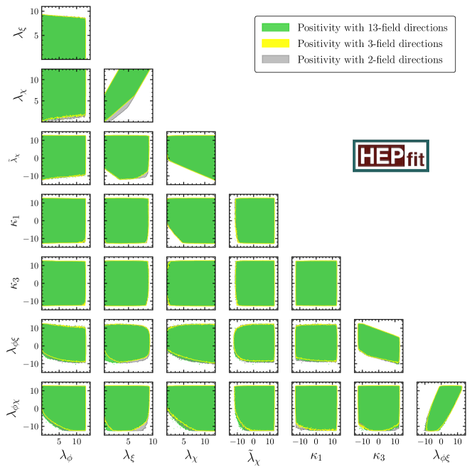
Figure 10: All possible quartic coupling planes in the eGM model with various BFB conditions. The grey (yellow) region shows the stability (BFB) of the potential in the 2-field (3-field) directions, while the green areas are allowed if we use BFB conditions on the full potential.

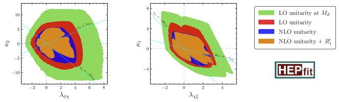
Figure 11: 99.7% CL allowed regions in the $\lambda_{i}$ vs. $\kappa_{j}$ planes. The green, red, and blue regions have the same meaning as in Figure 2. The brown areas show the parameter space without violating the perturbativity conditions ($R_{1}^{\prime}<1$) at one-loop level. The cyan dashed lines represent directions along which the tree-level amplitudes vanish.

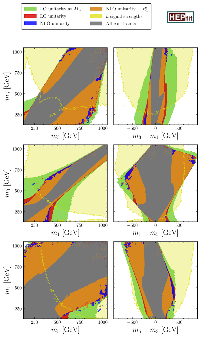
Figure 12: Allowed regions in the $m_{i}$ vs. $m_{j}$ ($m_{j}-m_{k}$) planes in the GM model. The color shaded regions have the same meaning as in Figure 6.

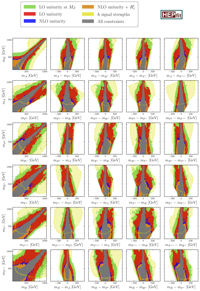
Figure 13: Allowed regions in the $m_{i}$ vs. $m_{j}$ ($m_{j}-m_{k}$) planes in the eGM model. The color shaded regions have the same meaning as in Figure 6.

References

- (1) ATLAS collaboration, Observation of a new particle in the search for the Standard Model Higgs boson with the ATLAS detector at the LHC, Phys. Lett. B 716 (2012) 1 [1207.7214].
- (2) CMS collaboration, Observation of a New Boson at a Mass of 125 GeV with the CMS Experiment at the LHC, Phys. Lett. B 716 (2012) 30 [1207.7235].
- (3) ATLAS, CMS collaboration, Measurements of the Higgs boson production and decay rates and constraints on its couplings from a combined ATLAS and CMS analysis of the LHC pp collision data at and 8 TeV, JHEP 08 (2016) 045 [1606.02266].
- (4) ATLAS collaboration, Measurement of the properties of Higgs boson production at TeV in the channel using fb-1 of collision data with the ATLAS experiment, JHEP 07 (2023) 088 [2207.00348].
- (5) ATLAS collaboration, Higgs boson production cross-section measurements and their EFT interpretation in the decay channel at 13 TeV with the ATLAS detector, Eur. Phys. J. C 80 (2020) 957 [2004.03447].
- (6) ATLAS collaboration, Measurements of Higgs boson production by gluon-gluon fusion and vector-boson fusion using decays in collisions at TeV with the ATLAS detector, Phys. Rev. D 108 (2023) 032005 [2207.00338].
- (7) ATLAS collaboration, Measurements of Higgs boson production cross-sections in the decay channel in pp collisions at = 13 TeV with the ATLAS detector, JHEP 08 (2022) 175 [2201.08269].
- (8) ATLAS collaboration, Measurements of Higgs bosons decaying to bottom quarks from vector boson fusion production with the ATLAS experiment at , Eur. Phys. J. C 81 (2021) 537 [2011.08280].
- (9) ATLAS collaboration, Measurements of and production in the decay channel in collisions at 13 TeV with the ATLAS detector, Eur. Phys. J. C 81 (2021) 178 [2007.02873].
- (10) ATLAS collaboration, Measurement of Higgs boson decay into -quarks in associated production with a top-quark pair in collisions at TeV with the ATLAS detector, JHEP 06 (2022) 097 [2111.06712].
- (11) ATLAS collaboration, A search for the dimuon decay of the Standard Model Higgs boson with the ATLAS detector, Phys. Lett. B 812 (2021) 135980 [2007.07830].
- (12) ATLAS collaboration, A search for the decay mode of the Higgs boson in collisions at = 13 TeV with the ATLAS detector, Phys. Lett. B 809 (2020) 135754 [2005.05382].
- (13) CMS collaboration, Measurements of Higgs boson production cross sections and couplings in the diphoton decay channel at = 13 TeV, JHEP 07 (2021) 027 [2103.06956].
- (14) CMS collaboration, Measurements of production cross sections of the Higgs boson in the four-lepton final state in proton–proton collisions at , Eur. Phys. J. C 81 (2021) 488 [2103.04956].
- (15) CMS collaboration, Measurements of the Higgs boson production cross section and couplings in the W boson pair decay channel in proton-proton collisions at , Eur. Phys. J. C 83 (2023) 667 [2206.09466].
- (16) CMS collaboration, Measurements of Higgs boson production in the decay channel with a pair of leptons in proton–proton collisions at TeV, Eur. Phys. J. C 83 (2023) 562 [2204.12957].
- (17) CMS collaboration, Measurement of the Higgs boson production via vector boson fusion and its decay into bottom quarks in proton-proton collisions at = 13 TeV, JHEP 01 (2024) 173 [2308.01253].
- (18) CMS collaboration, Evidence for Higgs boson decay to a pair of muons, JHEP 01 (2021) 148 [2009.04363].
- (19) CMS collaboration, Search for Higgs boson decays to a Z boson and a photon in proton-proton collisions at = 13 TeV, JHEP 05 (2023) 233 [2204.12945].
- (20) A. Banerjee, G. Bhattacharyya and N. Kumar, Impact of Yukawa-like dimension-five operators on the Georgi-Machacek model, Phys. Rev. D 99 (2019) 035028 [1901.01725].
- (21) A. Kundu, A. Le Yaouanc, P. Mondal and F. Richard, Searches for scalars at LHC and interpretation of the findings, in 2022 ECFA Workshop on e+e- Higgs/EW/Top factories, 11, 2022 [2211.11723].
- (22) P. Mondal, Enhancement of the W boson mass in the Georgi-Machacek model, Phys. Lett. B 833 (2022) 137357 [2204.07844].
- (23) T.-K. Chen, C.-W. Chiang and K. Yagyu, CP violation in a model with Higgs triplets, JHEP 06 (2023) 069 [2303.09294].
- (24) T.-K. Chen, C.-W. Chiang, S. Heinemeyer and G. Weiglein, 95 GeV Higgs boson in the Georgi-Machacek model, Phys. Rev. D 109 (2024) 075043 [2312.13239].
- (25) M. Chakraborti, D. Das, N. Ghosh, S. Mukherjee and I. Saha, New physics implications of vector boson fusion searches exemplified through the Georgi-Machacek model, Phys. Rev. D 109 (2024) 015016 [2308.02384].
- (26) A. Crivellin, S. Ashanujjaman, S. Banik, G. Coloretti, S.P. Maharathy and B. Mellado, Growing Evidence for a Higgs Triplet, 2404.14492.
- (27) C. Aime et al., Muon Collider Physics Summary, 2203.07256.
- (28) Muon Collider collaboration, The physics case of a 3 TeV muon collider stage, 2203.07261.
- (29) M. Forslund and P. Meade, High precision higgs from high energy muon colliders, JHEP 08 (2022) 185 [2203.09425].
- (30) CMS collaboration, Observation of electroweak production of same-sign W boson pairs in the two jet and two same-sign lepton final state in proton-proton collisions at 13 TeV, Phys. Rev. Lett. 120 (2018) 081801 [1709.05822].
- (31) CMS collaboration, Measurements of production cross sections of polarized same-sign W boson pairs in association with two jets in proton-proton collisions at 13 TeV, Phys. Lett. B 812 (2021) 136018 [2009.09429].
- (32) ATLAS collaboration, Search for doubly charged scalar bosons decaying into same-sign boson pairs with the ATLAS detector, Eur. Phys. J. C 79 (2019) 58 [1808.01899].
- (33) ATLAS collaboration, Measurement and interpretation of same-sign boson pair production in association with two jets in collisions at TeV with the ATLAS detector, 2312.00420.
- (34) M. Ciuchini, E. Franco, S. Mishima and L. Silvestrini, Electroweak Precision Observables, New Physics and the Nature of a 126 GeV Higgs Boson, JHEP 08 (2013) 106 [1306.4644].
- (35) K. Hartling, K. Kumar and H.E. Logan, Indirect constraints on the Georgi-Machacek model and implications for Higgs boson couplings, Phys. Rev. D 91 (2015) 015013 [1410.5538].
- (36) J. de Blas, M. Ciuchini, E. Franco, S. Mishima, M. Pierini, L. Reina et al., Electroweak precision observables and Higgs-boson signal strengths in the Standard Model and beyond: present and future, JHEP 12 (2016) 135 [1608.01509].
- (37) J. de Blas, M. Pierini, L. Reina and L. Silvestrini, Impact of the Recent Measurements of the Top-Quark and W-Boson Masses on Electroweak Precision Fits, Phys. Rev. Lett. 129 (2022) 271801 [2204.04204].
- (38) Particle Data Group collaboration, Review of Particle Physics, PTEP 2022 (2022) 083C01.
- (39) H. Georgi and M. Machacek, Doubly charged Higgs bosons, Nucl. Phys. B 262 (1985) 463.
- (40) M.S. Chanowitz and M. Golden, Higgs Boson Triplets With M () = M () , Phys. Lett. B 165 (1985) 105.
- (41) J.F. Gunion, R. Vega and J. Wudka, Naturalness problems for rho = 1 and other large one loop effects for a standard model Higgs sector containing triplet fields, Phys. Rev. D 43 (1991) 2322.
- (42) C. Englert, E. Re and M. Spannowsky, Pinning down Higgs triplets at the LHC, Phys. Rev. D 88 (2013) 035024 [1306.6228].
- (43) M. Garcia-Pepin, S. Gori, M. Quiros, R. Vega, R. Vega-Morales and T.-T. Yu, Supersymmetric Custodial Higgs Triplets and the Breaking of Universality, Phys. Rev. D 91 (2015) 015016 [1409.5737].
- (44) A. Kundu, P. Mondal and P.B. Pal, Custodial symmetry, the Georgi-Machacek model, and other scalar extensions, Phys. Rev. D 105 (2022) 115026 [2111.14195].
- (45) B.W. Lee, C. Quigg and H.B. Thacker, The Strength of Weak Interactions at Very High-Energies and the Higgs Boson Mass, Phys. Rev. Lett. 38 (1977) 883.
- (46) S. Dawson and S. Willenbrock, Unitarity constraints on heavy higgs bosons, Phys. Rev. Lett. 62 (1989) 1232.
- (47) L. Durand, J.M. Johnson and J.L. Lopez, Perturbative unitarity and high-energy W(L)+-, Z(L), H scattering. One loop corrections and the Higgs boson coupling, Phys. Rev. D 45 (1992) 3112.
- (48) P.N. Maher, L. Durand and K. Riesselmann, Two loop renormalization constants and high-energy 2 — 2 scattering amplitudes in the Higgs sector of the Standard Model, Phys. Rev. D 48 (1993) 1061 [hep-ph/9303233].
- (49) L. Durand, P.N. Maher and K. Riesselmann, Two loop unitarity constraints on the Higgs boson coupling, Phys. Rev. D 48 (1993) 1084 [hep-ph/9303234].
- (50) B. Grinstein, C.W. Murphy and P. Uttayarat, One-loop corrections to the perturbative unitarity bounds in the CP-conserving two-Higgs doublet model with a softly broken symmetry, JHEP 06 (2016) 070 [1512.04567].
- (51) V. Cacchio, D. Chowdhury, O. Eberhardt and C.W. Murphy, Next-to-leading order unitarity fits in Two-Higgs-Doublet models with soft breaking, JHEP 11 (2016) 026 [1609.01290].
- (52) M. Aoki and S. Kanemura, Unitarity bounds in the Higgs model including triplet fields with custodial symmetry, Phys. Rev. D 77 (2008) 095009 [0712.4053].
- (53) K. Hartling, K. Kumar and H.E. Logan, The decoupling limit in the Georgi-Machacek model, Phys. Rev. D 90 (2014) 015007 [1404.2640].
- (54) C.-W. Chiang, G. Cottin and O. Eberhardt, Global fits in the Georgi-Machacek model, Phys. Rev. D 99 (2019) 015001 [1807.10660].
- (55) C.-W. Chiang and K. Yagyu, Testing the custodial symmetry in the Higgs sector of the Georgi-Machacek model, JHEP 01 (2013) 026 [1211.2658].
- (56) C.-W. Chiang, A.-L. Kuo and T. Yamada, Searches of exotic Higgs bosons in general mass spectra of the Georgi-Machacek model at the LHC, JHEP 01 (2016) 120 [1511.00865].
- (57) K. Kannike, Vacuum stability conditions from copositivity criteria, Eur. Phys. J. C 72 (2012) 2093 [1205.3781].
- (58) J. Chakrabortty, P. Konar and T. Mondal, Copositive Criteria and Boundedness of the Scalar Potential, Phys. Rev. D 89 (2014) 095008 [1311.5666].
- (59) K. Kannike, Vacuum Stability of a General Scalar Potential of a Few Fields, Eur. Phys. J. C 76 (2016) 324 [1603.02680].
- (60) M. Abud and G. Sartori, The geometry of orbit-space and natural minima of higgs potentials, Physics Letters B 104 (1981) 147.
- (61) J. Kim, General Method for Analyzing Higgs Potentials, Nucl. Phys. B 196 (1982) 285.
- (62) M. Abud and G. Sartori, The Geometry of Spontaneous Symmetry Breaking, Annals Phys. 150 (1983) 307.
- (63) I.P. Ivanov, Minkowski space structure of the Higgs potential in 2HDM, Phys. Rev. D 75 (2007) 035001 [hep-ph/0609018].
- (64) A. Degee, I.P. Ivanov and V. Keus, Geometric minimization of highly symmetric potentials, JHEP 02 (2013) 125 [1211.4989].
- (65) K.G. Klimenko, On Necessary and Sufficient Conditions for Some Higgs Potentials to Be Bounded From Below, Theor. Math. Phys. 62 (1985) 58.
- (66) K.G. Murty and S.N. Kabadi, Some np-complete problems in quadratic and nonlinear programming, Math. Program. 39 (1987) 117–129.
- (67) I.P. Ivanov, M. Köpke and M. Mühlleitner, Algorithmic boundedness-from-below conditions for generic scalar potentials, Eur. Phys. J. C 78 (2018) 413 [1802.07976].
- (68) C. Bonilla, R.M. Fonseca and J.W.F. Valle, Consistency of the triplet seesaw model revisited, Phys. Rev. D 92 (2015) 075028 [1508.02323].
- (69) S. Blasi, S. De Curtis and K. Yagyu, Effects of custodial symmetry breaking in the Georgi-Machacek model at high energies, Phys. Rev. D 96 (2017) 015001 [1704.08512].
- (70) M.E. Krauss and F. Staub, Perturbativity Constraints in BSM Models, Eur. Phys. J. C 78 (2018) 185 [1709.03501].
- (71) G. Moultaka and M.C. Peyranère, Vacuum stability conditions for Higgs potentials with triplets, Phys. Rev. D 103 (2021) 115006 [2012.13947].
- (72) L. Durand, J.M. Johnson and J.L. Lopez, Perturbative unitarity and high-energy , , scattering. one-loop corrections and the higgs-boson coupling, Phys. Rev. D 45 (1992) 3112.
- (73) M.S. Chanowitz and M.K. Gaillard, The TeV Physics of Strongly Interacting W’s and Z’s, Nucl. Phys. B 261 (1985) 379.
- (74) J. Bagger and C. Schmidt, Equivalence theorem redux, Phys. Rev. D 41 (1990) 264.
- (75) B.W. Lee, C. Quigg and H.B. Thacker, Weak Interactions at Very High-Energies: The Role of the Higgs Boson Mass, Phys. Rev. D 16 (1977) 1519.
- (76) S. Dawson and S. Willenbrock, Radiative corrections to longitudinal-vector-boson scattering, Phys. Rev. D 40 (1989) 2880.
- (77) B. Keeshan, H.E. Logan and T. Pilkington, Custodial symmetry violation in the Georgi-Machacek model, Phys. Rev. D 102 (2020) 015001 [1807.11511].
- (78) S. Blasi, S. De Curtis and K. Yagyu, Effects of custodial symmetry breaking in the Georgi-Machacek model at high energies, Phys. Rev. D 96 (2017) 015001 [1704.08512].
- (79) C.W. Murphy, NLO Perturbativity Bounds on Quartic Couplings in Renormalizable Theories with -like Scalar Sectors, Phys. Rev. D 96 (2017) 036006 [1702.08511].
- (80) J. De Blas et al., HEPfit: a code for the combination of indirect and direct constraints on high energy physics models, Eur. Phys. J. C 80 (2020) 456 [1910.14012].
- (81) A. Caldwell, D. Kollar and K. Kroninger, BAT: The Bayesian Analysis Toolkit, Comput. Phys. Commun. 180 (2009) 2197 [0808.2552].
- (82) ATLAS, CMS collaboration, Combined Measurement of the Higgs Boson Mass in Collisions at and 8 TeV with the ATLAS and CMS Experiments, Phys. Rev. Lett. 114 (2015) 191803 [1503.07589].
- (83) D. Chowdhury and O. Eberhardt, Update of Global Two-Higgs-Doublet Model Fits, JHEP 05 (2018) 161 [1711.02095].
- (84) C. Englert, E. Re and M. Spannowsky, Triplet Higgs boson collider phenomenology after the LHC, Phys. Rev. D 87 (2013) 095014 [1302.6505].
- (85) L. Sartore and I. Schienbein, PyR@TE 3, Comput. Phys. Commun. 261 (2021) 107819 [2007.12700].
- (86) J. F. Gunion, H. E. Haber, G. L. Kane and S. Dawson, The Higgs Hunter’s Guide, Front. Phys. 80 (2000) 1–404.
- (87) N.D. Christensen and C. Duhr, FeynRules - Feynman rules made easy, Comput. Phys. Commun. 180 (2009) 1614 [0806.4194].
- (88) T. Hahn, Generating Feynman diagrams and amplitudes with FeynArts 3, Comput. Phys. Commun. 140 (2001) 418 [hep-ph/0012260].
- (89) M.-x. Luo and Y. Xiao, Two loop renormalization group equations in the standard model, Phys. Rev. Lett. 90 (2003) 011601 [hep-ph/0207271].
- (90) D. Chowdhury and O. Eberhardt, Global fits of the two-loop renormalized Two-Higgs-Doublet model with soft Z2 breaking, JHEP 11 (2015) 052 [1503.08216].