The Impact of COVID-19 on Co-authorship and Economics Scholars’ Productivity

Abstract

The COVID-19 pandemic has disrupted traditional academic collaboration patterns, prompting a unique opportunity to analyze the influence of peer effects and coauthorship dynamics on research output. Using a novel dataset, this paper endeavors to make a first cut at investigating the role of peer effects on the productivity of economics scholars, measured by the number of publications, in both pre-pandemic and pandemic times. Results show that peer effect is significant for the pre-pandemic time but not for the pandemic time. The findings contribute to our understanding of how research collaboration influences knowledge production and may help guide policies aimed at fostering collaboration and enhancing research productivity in the academic community.

Keywords COVID-19  $\cdot$ Productivity  $\cdot$ Co-authorship  $\cdot$ Game Theory  $\cdot$ Publication

1 Introduction

Academic productivity is commonly used in academic hiring and promotion decisions, as well as in evaluations of research programs and departments [1, 2], because a higher number of publications may indicate that the scholar has been active in research and has made significant contributions to the field. In recent years, there has been a growing interest in understanding the factors that contribute to the productivity of scholars in various disciplines. Among these factors, the role of peer effects and co-authorship has emerged as an area of significant importance [3]. Scholars who have strong social networks and interactions with colleagues in their field may publish more, because they have access to more resources, including research funding, data, and other research materials. Co-authorship also facilitates knowledge sharing, which could lead to new research ideas and opportunities for publication. For example, [4] demonstrates that one single strong connection could have a substantial and positive influence on the scholar’s productivity and citation rates.

The COVID-19 pandemic has fundamentally altered the way we live, work, and collaborate. As the pandemic forced the closure of universities and research institutions, it inadvertently reshaped the landscape of academic research. Consequently, this unprecedented situation presents a unique opportunity to examine the peer effects and co-authorship dynamics among economics scholars in both pre-pandemic and pandemic times. Working at home may reshape scholars’ way of writting, communication, and collaboration. On one hand, scholars have more flexible schedules and greater autonomy over their work. It provides opportunities for virtual collaboration through video conferencing and instant messaging among scholars who locate in different regions or time zones. On the other hand, scholars who work from home may experience greater isolation and have less opportunity for informal interactions and discussions with their co-authors. It may also create distractions and disruptions, such as balancing work responsibilities with home responsibilities.

This paper employs a novel dataset, collected from Google Scholar, that includes scholarly literature and co-authorship networks of economics scholars. We empirically estimate the peer effect of economic scholars on their number of publications during both the pre-pandemic and pandemic periods. The present study is important for several reasons. First, understanding the role of co-authorship in academic productivity provides insights into how research collaborations influence knowledge production and dissemination. Second, by comparing pre-pandemic and pandemic times, this study offers a better understanding of how the COVID-19 crisis has affected academic collaboration patterns and the overall productivity of scholars in the field of economics. Finally, the findings of this study may help guide policies aimed at fostering collaboration and enhancing research productivity in the academic community.

This paper is organized as follows. Section 2 reviews the relevant literature on peer effects and academic productivity. Section 3 describes the data and provides summary statistics. Section 4 presents the model framework and empirical strategy, while Section 5 discusses the main results. Finally, Section 6 concludes and offers directions for future research.

2 Literature Reivew

From the methodological perspective, our work is closely related to two main strands of the literature. Firstly, fast-growing literature on peer effects in networks. As reflected by [5], there are two different impacts from peers. One is endogenous peer effects which are the impact of peers’ outcomes and the other are contextual peer effects, which are the impact of peers’ characteristics. Distinguishing these impacts may be impossible because of the simultaneity in the behavior of interacting agents. [6, 7, 8, 9] are the initial studies of network interactions. For example, [6] builds the benchmark linear-in-means model of peer effects and describes the identification conditions when agents interact through a network assuming peers of peers are not peers. The assumption that the agents’ characteristics have an impact on individual outcomes only through their effect on peers’ outcomes, provides valid instruments addressing correlated effects. Therefore, endogenous and contextual peer effects are identified. An important insight is that identification depends on the structure of the network itself. [10, 11, 12, 13] investigate heterogeneous peer effects, in which men and women are subject to different peer effects. Individuals could also be subject to different effects from male peers and from female peers, which potentially leads to endogenous peer effects. Concerning heterogeneity of peer effects, [14] incorporates heterogeneity analysis by assuming that endogenous peer effect coefficients are random in a linear-in-means model. He shows these random endogenous peer effects can be point-identified if there is no contextual peer effect for an exogenous characteristic.

The second strand of literature is related to tackling the problem of correlated effects and exploiting the identification possibilities generated by interaction networks. In the literature, researchers have developed at least four broad strategies to address this correlated effects issue: random peers, random shocks, structural endogeneity, and panel data. The first strategy is random peers, who are randomly allocated through natural or designed experiments. For example, [15] looks at Dartmouth College roommates in pairs, triples, or quads among students. [16] randomly match workers in pairs in the lab. [7] look at the choice of a major among Bocconi undergraduates. The insight is with random peers an agent’s observed and unobserved characteristics are uncorrelated with their peers’ observed and unobserved characteristics. The second strategy is random shocks. For instance, [17] uses exogenous variations to study treatment randomization which allows researchers to identify the causal impacts of the treatment and peers’ treatments and peers’ outcomes even when the network is endogenous within a linear-in-means framework. [18, 19, 20] study spillover effects. As an individual’s potential outcome may depend on the full vector of potential treatments, the causal impact of a randomized treatment cannot be estimated by simply computing the difference in average outcome among treated and untreated individuals. [21, 22] identify spillovers by assuming agents are organized in groups and that spillovers take place within, not between groups, then comparing the outcomes of untreated individuals in treated and untreated groups. The third strategy is called the structural framework. [23] first proposed the structural approach to address correlated effects issues. This approach provides a potentially powerful way to control for network endogeneity in peer effect regressions, reminiscent of Heckman’s correction for sample network formation simultaneously may allow researchers to recover information on common unobservables. The fourth strategy on peer effects in networks applies to panel data. However, this literature is scarce. A few papers analyze peer effects utilizing panel data, see [24, 25, 26]. These studies have introduced individual fixed effects but do not address contextual peer effects associated with time-invariant characteristics. We view this as a potentially important limitation of these frameworks and thus is an important future research question.

The model that is employed in the present study belongs to the structural endogeneity framework. It relates to the models that use static games with incomplete information in which, agents act non-cooperatively, see [27, 28]. The assumption of incomplete information of the peer effect models for discrete outcomes is broadly studied, for instance, [29, 30, 31, 32]. In the literature, agent $i$’s decision is influenced by their own observable characteristics, unobservable individual type, and other agents’ choice. The recent study from [33, 34] propose methods to estimate the network’s probability distribution using cross-sectional data when the network is imperfectly observed. They construct a network game, and each agent chooses an integer outcome to maximize his or her preference, which contains observed characteristics of the agent and the peers, the difference between the choice of the agent and the peers, a cost function, and a private signal. They prove that under a few assumptions, there is a unique Bayesian Nash Equilibrium for this game, and an estimator is proposed based on pseudo-likelihood maximization.

The literature of empirical papers exploring the relationship between co-authorship and academic productivity has expanded recently. Nonetheless, consensus remains elusive regarding whether this relationship is positive, negative, or insignificant. For example, [35] demonstrates that economists who are more collaborative are also more productive. Factors such as tenure, age, and geographical variables do not have a significant impact on productivity. [36] also finds a positive correlation between intellectual collaboration and individual performance, after accounting for endogenous network formation, unobservable heterogeneity, and factors that vary over time. As indirect evidence, [37] identifies that, at the individual level, the average publication quality rises with the average number of authors per paper, individual field diversity, the total number of published papers, and the presence of foreign co-authors. Female and older academics tend to publish less frequently. Conversely, some scholars argue that the relationship between co-authorship and productivity exhibits a negative correlation or lacks statistical significance. [38] discovers that for a specific scholar, increased co-authorship leads to higher quality, longer, and more frequent publications. However, after adjusting for the number of authors, the relationship between co-authorship and a scholar’s attributable output becomes negative. Other research contends that after controlling for article length, journal and author quality, and subject area, scholar fixed effects, the productivity of prior collaborators is not a significant determinant of a researcher’s own productivity [39], or higher quality research [40]. [41] finds that coauthors of highly helpful scientists that die experience a decrease in output quality but not output quantity.

3 Economic Scholars Data

The Economic scholars dataset consists of 1,671 core faculties from the best 50 Economics Schools in the United States based on US News in 2022, who have registered themselves a homepage on Google Scholar. The dataset does not include visiting professors, teaching professors, or lecturers. The homepage provides rich information on the individual’s influences and research journey in academia. Besides the names and affiliations, scholars may list their research interests and sub-fields at the head of the page. On the right-hand side, the scholar’s cumulative citations, H-index, and I10 index are shown, along with regular coauthors and the histogram of the number of citations and publications each year for the last 10 years. On the left-hand side, a comprehensive list of academic output of the scholar’s could be viewed, including the paper’s title, journal, authors, year, and the number of citations. See a snapshot of the Google Scholar homepage in the figure below.

Figure 1: Google Scholar Homepage Example

A key feature of the data collected from Google Scholar is its comprehensiveness. The website aggregates information from a wide range of sources, including journal articles, conference papers, theses and dissertations, technical reports, books and book chapters, patents, working papers, and repositories. Thus compared to using data sources from academic journals, the lagged effect of co-authorship on scholars’ academic output due to journals’ reviewing process could be largely alleviated.

Based on scholars’ publications, we construct an economics scholar co-authorship network each year for the last 10 years. Each node represents a faculty member in the economics department, and there is an edge between any two nodes if they have co-authored at least one paper in a given year. The edge density of a temporal network indicates the prevalence of scholar collaborations in that year, or the percentage of observed co-authorships over all possible collaborations between any two scholars. Economic scholars’ productivity, revealed by the annual average numbers of publications, gradually increase since 2013, experience a surge and reaches the top in 2020, then falls back slowly in 2021 and 2022. Network edge density reaches its highest level in 2018, then declines and reaches the bottom in 2020, before it bounces back in 2021 and 2022. Interestingly, scholars’ average productivity moves in the same direction as the prevalence of collaborations before 2018, but in the opposite direction from 2019 to 2021.

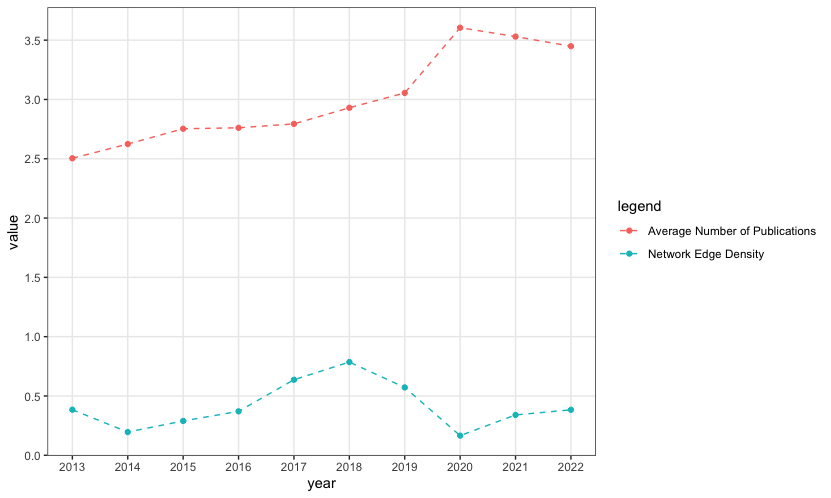
Figure 2: Average Number of Publications and Edge Density by Year

The experience of economic faculties in academia is 25 years on average as of 2023, which is measured by the difference between 2022 and the year of the scholar’s first published article on Google Scholar. African American scholars, identified either directly by their listed nationality in CV or indirectly by the combination of the predicted country of origin using names and faculty pictures, account for 0.9% of the economics faculty. 18% of the faculty in the sample are female. We also label the expertise of economic scholars with their listed sub-fields on the Google homepage. For those who have left the section blank, We fill in the missing values by the fields that are shown on the department faculty website and the scholar’s curriculum vitae. The sub-fields are not mutually exclusive, and it is reasonable for scholars to have two, three, or more specialties. For example, a macroeconomist may specify econometrics, monetary policy, international economics, or finance as the expertise as well. In our sample, economic/econometrics theory, macroeconomics, and labor economics are the three top fields that scholars may work on, followed by econometrics, industrial organization, and development economics.

Table 1: Summary Statistics of Economics Scholars

Statistic	Mean	St. Dev.	Min	Median	Max
Years in Academia	24.96	15.97	1	22	72
African American	0.009	0.09	0	0	1
Female	0.18	0.39	0	0	1
Number of Publications in 2013	2.504	3.154	0	2	25
Number of Publications in 2014	2.624	3.195	0	2	30
Number of Publications in 2015	2.75	3.38	0	2	27
Number of Publications in 2016	2.76	3.31	0	2	21
Number of Publications in 2017	2.79	3.45	0	2	40
Number of Publications in 2018	2.93	3.43	0	2	40
Number of Publications in 2019	3.06	3.84	0	2	33
Number of Publications in 2020	3.61	4.93	0	2	68
Number of Publications in 2021	3.53	4.46	0	2	55

Table 2: Sub-fields of Economics Scholars

	Economics Sub-field (%)
Theory	18.25
Macroeconomics	19.80
Labor Economics	18.01
Econometrics	15.92
Industrial Organization	11.31
Development Economics	11.61
Health Economics	7.60
Financial Economics	10.29

4 Network Game with Peer Effects and Incomplete Information

Following the notation in [34], suppose there is a population of $n$ agents that interact through a network matrix $\mathbf{G}$ with zero diagonal and non-negative elements $g_{ij}$ that represents the proximity of $i$ and $j$. Each agent $i$ chooses an integer outcome, $y_{i}$, to maximize his or her individual utility:

$$U_{i}\left(y_{i},\mathbf{y}_{-i}\right)=\psi_{i}y_{i}-c\left(y_{i}\right)-\frac{\lambda}{2}\left(y_{i}-\bar{y_{i}}\right)^{2}+e_{i}\left(y_{i}\right)$$

In the equation, $\mathbf{y}_{-i}=\left(y_{1},\cdots,y_{i-1},y_{i+1},\cdots,y_{n}\right)$. Observable characteristics of $i$ and his or her peers is contained in $\psi_{i}=\mathbf{x}_{i}\mathbf{{}^{\prime}\beta}+\mathbf{\bar{x_{i}}^{\prime}\gamma}$, where $\mathbf{x}_{i}$ is the vector of the agent’s observable characteristics and $\mathbf{\bar{x_{i}}}$ is the average characteristics of the peers. Own effects $\mathbf{\beta}$ and contextual effects $\mathbf{\gamma}$ are parameters to be estimated. Function $c\left(\cdot\right)$ captures the cost of choosing $y_{i}$, and $\bar{y_{i}}=\sum_{j=1}^{n}g_{ij}y_{j}$. The peer effect, $\lambda\geq 0$, is designed to show conformity so that $\frac{\lambda}{2}\left(y_{i}-\bar{y_{i}}\right)^{2}$ represents the social cost that is greater if the difference between the choice of agent $i$ and his or her peers is larger. $\left(e_{i}\left(r\right)\right)_{r\in\mathbb{N}}$ is a random variable sequence that indicates the agent’s private type. The value is observable to $i$ for any $r\in\mathbb{N}$, but not to other agents. Since the types and thus the choices of other agents are not observable, agent $i$ would maximize the expectation of his or her preferences conditional on the information set $I_{i}=\left\{\psi_{i},\mathbf{\psi}_{-i},\mathbf{g}_{i},\mathbf{G}_{-i}\right\}$:

$$U_{i}^{e}\left(y_{i}\right)=\psi_{i}y_{i}-c\left(y_{i}\right)-\frac{\lambda}{2}\mathbb{E}_{\bar{y_{i}}|I_{i}}\left[\left(y_{i}-\bar{y_{i}}\right)^{2}\right]+e_{i}\left(y_{i}\right)$$

Define $\Delta$ as the first difference operator. It is proved in [34] that under the following three assumptions, there is a unique integer $r_{0}$ that maximizes the preference $U_{i}^{e}\left(\cdot\right)$, and $U_{i}^{e}\left(r\right)\geq\max\left\{U_{i}^{e}\left(r-1\right),U_{i}^{e}\left(r+1\right)\right\}$ if and only if $r=r_{0}$:

Assumption 1.

$c(\cdot)$ is a strictly convex and increasing function.

Assumption 2.

For any $r\in\mathbb{N}$, $e_{i}\left(r\right)=e_{i}\left(r-1\right)+\epsilon_{i}$, where $\epsilon_{i}|I_{i}$ are independent and identically follow a continuous symmetric distribution with cdf function $F_{\epsilon|I}$, and pdf function $f_{\epsilon|I}$.

Assumption 3.

$\lim\limits_{r\to\infty}r^{-\rho}\left(\Delta c(r+1)-\Delta c(r)\right)>0$, and $f_{\epsilon|I}(x)=o(|x|^{-\kappa})$ at $\infty$, where $\rho\geq 0$, $(1+\rho)(\kappa-1)>2$.

The first assumption implies that $\Delta c(r+1)-\Delta c(r)>0$. The expected payoff is strictly concave and has a global maximum that could be reached at a single point. The second assumption suggests that agents consider the same information $\epsilon_{i}$ for any additional $r$ so that $\Delta e_{i}(r)$ does not depend on $y_{i}$. The third assumption suggests that when $y_{i}$ is sufficiently high, the cost increases at a minimum rate. The tail of $f_{\epsilon|I}(x)$ needs to decay, and the trade-off condition between $\rho$ and $\kappa$ guarantees that when $r\rightarrow\infty$, the probability of $y_{i}=r$ converges to $0$ at some rate.

Agent $i$ chooses $r$ if and only if $U_{i}^{e}\left(r\right)\geq U_{i}^{e}\left(r-1\right)$ and $U_{i}^{e}\left(r\right)\geq U_{i}^{e}\left(r+1\right)$. Substituting $U_{i}^{e}\left(\cdot\right)$ and $e_{i}\left(\cdot\right)$ into the two conditions, we have $-\psi_{i}-\lambda\bar{y_{i}}^{e}+a_{r}\leq\epsilon_{i}\leq-\psi_{i}-\lambda\bar{y_{i}}^{e}+a_{r+1}$, where $a_{r}=\Delta c(r)+\lambda r-\frac{\lambda}{2}$, $\bar{y_{i}}^{e}=\sum_{j=1}^{n}g_{ij}y_{j}^{e}$, $y_{i}^{e}$ is agent $i$’s rational expected choice conditional on information set $I_{i}$. The probability of agent $i$ choosing $r$, $p_{ir}$, could readily be written as:

$$p_{ir}=F_{\epsilon|I}\left(\lambda\bar{y_{i}}^{e}+\psi_{i}-a_{r}\right)-F_{\epsilon|I}\left(\lambda\bar{y_{i}}^{e}+\psi_{i}-a_{r+1}\right)$$

The expected outcome associate with the belief system $\mathbf{p}=(p_{ir})$ could be written as $y_{i}^{e}=\sum_{r=1}^{\infty}rp_{ir}=\sum_{r=1}^{\infty}F_{\epsilon|I}\left(\lambda\bar{y_{i}}^{e}+\psi_{i}-a_{r}\right)$. Although the expected payoff has a global maximum, it is possible that there are multiple expected outcomes and belief systems $\mathbf{p}$. To avoid the multiple rational expected equilibria issue, a threshold for the peer effect needs to be imposed:

Assumption 4.

$\lambda<B_{c}/||\mathbf{G}||_{-\infty}$, where $B_{c}=\left(\max_{u\in\mathbb{R}}\sum_{r=1}^{\infty}f_{\epsilon|I}\left(u-a_{r}\right)\right)^{-1}$

With the above four assumptions, this game is proved to have a unique Bayesian Nash Equilibrium given by $\mathbf{y^{*}}=(y_{1}^{*},\cdots,y_{n}^{*})^{\prime}$, where $y_{i}^{*}$ is the maximizer of the expected payoff $U_{i}^{e}\left(\cdot\right)$.

In the payoff function $\psi_{i}=\mathbf{x}_{i}\mathbf{{}^{\prime}\beta}+\mathbf{\bar{x_{i}}^{\prime}\gamma}$, let the observable characteristics of agent $i$ and the peers, $\mathbf{x}_{i}$ and $\mathbf{\bar{x_{i}}}$, be $1\times K$ vectors. Specify $\mathbf{X}=\left[\mathbf{x}_{1},\cdots,\mathbf{x}_{n}\right]^{\prime}$ as a $n\times K$ matrix, and $\mathbf{\psi=Z\Gamma}$ where $\mathbf{Z}=\left[\mathbf{X\ GX}\right]$ and $\mathbf{\Gamma}=\left(\mathbf{\beta}^{\prime},\mathbf{\gamma}^{\prime}\right)^{\prime}$. Define $\delta_{r}=a_{r}-a_{r-1}$ for $r\geq 2$ and $\delta_{1}=0$. As $a_{r}=\Delta c(r)+\lambda r-\frac{\lambda}{2}$, $\delta_{r}=\Delta\Delta c(r)+\lambda$ for $r\geq 2$. Since $c(\cdot)$ is non-parametric, an infinite number of $\delta_{r}$ needs to be estimated. For identification purposes, the paper assumes the limitation in Assumption 3 is reached for large $r$:

Assumption 5.

There exists a positive constant $R$, such that $\forall r>R$, $\delta_{r}=(r-1)^{\rho}\bar{\delta}+\lambda$, where $\bar{\delta}>0$, $\rho>0$.

The probability of agent $i$ choosing $r$ could then be re-written as:

$$p_{ir}=F_{\epsilon|I}\left(\lambda\bar{y_{i}}^{e}+\mathbf{z}_{i}^{\prime}\mathbf{\Gamma}-a_{r}\right)-F_{\epsilon|I}\left(\lambda\bar{y_{i}}^{e}+\mathbf{z}_{i}^{\prime}\mathbf{\Gamma}-a_{r+1}\right)$$

where $\mathbf{z}_{i}^{\prime}$ is $\mathbf{Z}$’s $i$-th row, $a_{0}=-\infty$, $a_{r}=a_{1}+\sum_{k=1}^{r}\delta_{k}$ for all $r\geq 1$, $\delta_{1}=0$, $\delta_{r}=(r-1)^{\rho}\bar{\delta}+\lambda$ for all $r>R$. Let $\bar{R}$ be the smallest $R$ for which Assumption 5 holds. It is shown that under a few additional assumptions, if $F_{\epsilon}$ is known, then $\lambda,\mathbf{\Gamma},\mathbf{\delta},\bar{\delta},\rho$ are point identified.

Parameter estimation proceeds with a likelihood approach. Assume $\epsilon_{i}$ follows a standard normal distribution, then the probability $p_{ir}$ would be:

$$p_{ir}=\Phi\left(\lambda\mathbf{g}_{i}\mathbf{y}^{e}+\mathbf{z}_{i}^{\prime}\mathbf{\Gamma}-a_{r}\right)-\Phi\left(\lambda\mathbf{g}_{i}\mathbf{y}^{e}+\mathbf{z}_{i}^{\prime}\mathbf{\Gamma}-a_{r+1}\right)$$

where $\Phi(\cdot)$ is the CDF of standard normal distribution, $\mathbf{L}$ is a mapping, $\mathbf{y}^{e}=\mathbf{L}(\mathbf{\theta,y}^{e})=(l_{1}(\mathbf{\theta},\mathbf{y}^{e}),\cdots,l_{n}(\mathbf{\theta},\mathbf{y}^{e}))^{\prime}$, and $l_{i}(\mathbf{\theta},\mathbf{y}^{e})=\sum_{r=1}^{\infty}\Phi\left(\lambda\mathbf{g}_{i}\mathbf{y}^{e}+\mathbf{z}_{i}^{\prime}\mathbf{\Gamma}-a_{r}\right)$. For any fixed $\bar{R}$, since $\mathbf{y}^{e}$ is not observed, it needs to be computed for every value of $\mathbf{\theta}$. Alternatively, the parameters could be estimated using the NPL algorithm in [42], which takes advantage of an iterative process. The algorithm maximizes a pseudo-likelihood function:

$$L_{n}\left(\mathbf{\theta,y}^{e}\right)=\frac{1}{n}\sum_{i=1}^{n}\sum_{r=0}^{\infty}d_{ir}log(p_{ir})$$

where $\mathbf{\theta}=\left(log(\lambda),\mathbf{\Gamma}^{\prime},log(\tilde{\mathbf{\delta}}^{\prime}),log(\bar{\delta}),log(\rho)\right)^{\prime}$, $d_{ir}=1$ if $y_{i}=r$ and $0$ otherwise. It starts by guessing a set of initial probabilities for each agent’s choices, and then updating these probabilities in each iteration until the parameters and probabilities converge to a stable solution, e.g. $||\mathbf{\theta}_{(t)}-\mathbf{\theta}_{(t-1)}||_{1}$ and $||\mathbf{y}_{(t)}-\mathbf{y}_{(t-1)}||_{1}$ are less than $10^{-4}$.

The model also takes into account the endogeneity problem induced by agents’ unobserved characteristics. For instance, in our application, scholars’ familiarity with coding, or their extent to communicate with others could affect both which scholars they may collaborate with ($\mathbf{G}$) and their own number of publications ($\mathbf{y}$). Let the latent utility of scholar $i$ and $j$ being coauthors be $\mathbf{g}_{ij}^{*}=\mathbf{\ddot{x}}_{ij}\mathbf{\bar{\beta}}+\mu_{i}+\nu_{j}+\eta_{ij}$, where $\mathbf{\ddot{x}}_{ij}$ contains dyadic variables, $mu_{i}$ and $\nu_{j}$ are individual fixed effects. The probability of scholar $i$ and $j$ being coauthors could be modelled as:

$$P_{ij}=\mathbb{P}(\mathbf{g}_{ij}^{*}>0)=F_{\eta}\left(\mathbf{\ddot{x}}_{ij}\mathbf{\bar{\beta}}+\mu_{i}+\nu_{j}\right)$$

The fixed effects are assumed to be unobservable for the researcher, but observable for the scholars so that they are included in the information set.

Assumption 6.

For continuous function $h_{\epsilon}$, $\epsilon_{i}=h_{\epsilon}(\mu_{i},\nu_{i},\bar{\mu}_{i},\bar{\nu}_{i})+\epsilon_{i}^{*}$, where $\epsilon_{i}^{*}$ is independent of $\mathbf{Z}$ and $\mathbf{G}$, $\bar{\mu}_{i}=\sum_{j=1}^{n}\mathbf{g}_{ij}\mu_{j}$, $\bar{\nu}_{i}=\sum_{j=1}^{n}\mathbf{g}_{ij}\nu_{j}$.

The $\epsilon$ could be replaced by $h_{\epsilon}(\mu_{i},\nu_{i},\bar{\mu}_{i},\bar{\nu}_{i})+\epsilon_{i}^{*}$. Adapting Assumption 2 and Assumption 3 to $\epsilon_{i}^{*}$, the defined Bayesian Nash Equilibrium is still valid. The estimator computes $\hat{\mu}_{i}$ and $\hat{\nu}_{i}$ using a standard Logit in the first step, then substitute the estimated values for $\mu_{i}$ and $nu_{i}$ in the second step. Function $h_{\epsilon}$ is approximated using a sieve method. We refer readers that are interested in the model and technical details to the original paper [34].

The Economics scholar data contains the annual number of publications for each scholar from 2018 to 2021. We split the sample into pre-Covid and Covid periods by time (2018-2019, 2020-2021), and apply the model to each of these 2-year periods to estimate the peer effect. Specifically, We define $y_{i}$ as the total number of publications of scholar $i$ within each 2-year period. Data is segmented in this way because productivity and collaboration are observed to move in different directions before and after 2019. The pandemic and schools’ transition to virtual learning in 2020-2021 also inevitably affect scholars’ productivity and the way they collaborate, so the peer effect $\lambda$ is expected to have some change. We keep the length of each period the same to ensure that the estimated results in the two models are comparable. We include gender, an indicator for African American scholars, expertise, recent productivity indicated by the average number of publications of the scholar in the previous 3 years, total citations up to the first year of each period, and academic experience in the observable characteristics. We discretize scholars’ recent productivity, total citations, and academic experience, and set scholars with an average number of 0 or 1 publication in the previous 3 years, less than 100 citations up to the first year of each period, and less than 10 years of experience, as the reference levels respectively. In the presence of productivity rise during Covid times, we construct an additional Covid index for the period 2019-2021 in order to control for the extent to which the scholars’ publications after the outbreak of the epidemic are related to the Covid context. We use topic modeling to predict the topic of each paper published within these three years based on the title and abstract. The model is capable of recognizing papers that are inspired by the pandemic from other publications, see the table of predicted topics and the words with the highest conditional probability for each topic in the following table. We define a paper is Covid-related if its probability of belonging to the "Covid-19" topic is higher than 50%. The Covid index for each scholar is calculated as:

$$\text{Covid Index}=\frac{\text{Number of Covid-related Publications in 2019-2021}}{\text{Number of Publications in 2019-2021}}$$

The mean Covid index for economics scholars is 0.11, meaning that on average, 11% of the papers written in 2019-2021 by an economics faculty are inspired by the pandemic.

Table 3: Predicted Topics of Economic Publications in 2019-2021

Topic	Key Words	Percentage(%)
Covid-19	Covid-19, Health, Pandemic, Impact, Effects	26.05
Macro/Finance/International	Financial, Trade, Monetary, Policy, Experimental	19.97
Micro/Theory/Metrics/IO	Market, Theory, Labor, Learning, Estimation	27.81
Development/Social Science/Others	Inequality, Gender, Mobility, Work, Review	26.17

Social interaction matrix $\mathbf{G}$ is a row-normalized version of the adjacency matrix $\mathbf{W}=\left[w_{ij}\right]$, in which $w_{ij}=1$ if scholar $i$ and $j$ has collaborated on at least 2 papers within the 3-year period and $0$ otherwise. We rule out the case in which two scholars coauthored a single paper to focus on stable relationships. For example, if there are three scholars $i$, $j$ and $l$, scholar $i$ has worked with both $j$ and $l$ on more than one paper during the 3-year period. Then $\mathbf{G}$ is specified in the following way:

$$\mathbf{G}=\left[\begin{array}[]{ccc}0&\frac{1}{2}&\frac{1}{2}\\ 1&0&0\\ 1&0&0\\ \end{array}\right]$$

Each agent considers the average characteristics of his or her coauthors. For example, for the payoff function $U_{i}(y_{i})$ in the above example, $\bar{y}_{i}=\frac{1}{2}y_{j}+\frac{1}{2}y_{l}$. Peer effect $\lambda$ indicates how much "peer pressure" a scholar may have due to the difference between the scholar’s own productivity and the average productivity of the co-authors.

To account for the endogeneity of network formation, in the first stage, we estimate scholars’ unobserved characteristics using a dyadic Logit model. In the network formation model, from the school level, we control for homophily of the same department, and the same US News Ranking (Top 10, 11-20, 21-30, 31-40, 41-50). From the individual level, we consider the differences between the two scholars’ academic experience in years, total citations up to the first year of the period, the average number of publications each year during the previous three years, and the number of total publications. We include dummies to indicate whether the dyad involves at least one female author, and at least one African American scholar. We also control for the two scholars’ common research interests, measured by the number of fields that are listed on both scholars’ websites. In the second stage, We include individual fixed effects as additional control variables to evaluate the peer effect.

In practice, the value of $\bar{R}$ needs to be specified by the researcher in advance. Following the suggestion of the author, We experiment with the value of $\bar{R}$ by increasing it from $2$ until the change of the estimated parameters is not significant, or it reaches $\max(y)-2$. The estimation is done using the R package provided by the author.

5 Empirical Results

The estimated peer effect is significant for pre-Covid times (2018-2019), but not for Covid times (2020-2021). This implies that economic scholars exhibit conformity in the number of publications before the schools switch to virtual mode. However, there is a sign that while working at home, economic scholars are cooperating with a more diverse group of co-authors in terms of productivity, i.e. more collaborations among prolific scholars and scholars who publish less are expected. Recent productivity, represented by the scholar’s average number of publications during the previous 3 years, is an important predictor of a scholar’s productivity in the future. Scholars who are more prolific in the past 3 years would be more productive in the future. Compared to scholars whose total citations are below 2,000, scholars who have more citations are likely to publish more. Scholars’ years in academia significantly affect their productivity during Covid times. Emerging scholars produce relatively more than senior scholars. Gender plays a significant role only during the pre-Covid time.

Productivity is also related to the economics sub-fields that scholars work in. For example, econometricians publish relatively fewer papers in 2018-2019. Scholars who work in health economics are more prolific, and the effect is stronger during Covid times. The significant and positive Covid index implies that during 2019-2021, the higher proportion of a scholar’s papers is related to Covid, the more publications he or she would have. After controlling for the Covid index, the coefficient of scholars working in the field of health economics drops from $0.33$ to $0.30$.

For contextual effect, during Covid times, collaborating with macroeconomists and established scholars who have 100-2,000 citations help publish more papers.

Table 4: Peer Effect on Scholars’ Number of Publications in Non-Covid and Covid Times

	Pre-Covid	Covid	Covid + Covid Index
	(2018-2019)	(2020-2021)	(2020-2021)
$\lambda$	0.10∗∗∗	0.01	0.02
	(0.03)	(0.03)	(0.03)
Note:	∗p$<$0.1; ∗∗p$<$0.05; ∗∗∗p$<$0.01

Table 5: Own Effects on Scholars’ Number of Publications in Non-Covid and Covid Times

	Pre-Covid	Covid	Covid + Covid Index
	(2018-2019)	(2020-2021)	(2020-2021)
2-4 Publications Per Year	0.40∗∗∗	0.28∗∗∗	0.27∗∗∗
	(0.07)	(0.06)	(0.06)
5-9 Publications Per Year	1.22∗∗∗	1.17∗∗∗	1.17∗∗∗
	(0.09)	(0.09)	(0.09)
10+ Publications Per Year	2.38∗∗∗	2.46∗∗∗	2.46∗∗∗
	(0.16)	(0.16)	(0.16)
100-499 Citations	$-$0.15∗	$-$0.21∗∗	$-$0.21∗∗
	(0.08)	(0.09)	(0.09)
500-1,999 Citations	$-$0.02	$-$0.11	$-$0.11
	(0.07)	(0.07)	(0.07)
2,000-4,999 Citations	0.48∗∗∗	0.38∗∗∗	0.37∗∗∗
	(0.09)	(0.10)	(0.10)
5,000-9,999 Citations	0.71∗∗∗	0.59∗∗∗	0.58∗∗∗
	(0.13)	(0.13)	(0.13)
10,000-19,999 Citations	0.77∗∗∗	0.86∗∗∗	0.84∗∗∗
	(0.15)	(0.14)	(0.14)
20,000+ Citations	1.81∗∗∗	1.53∗∗∗	1.52∗∗∗
	(0.18)	(0.16)	(0.16)
Experience 10-20 Years	$-$0.01	$-$0.12	$-$0.11
	(0.08)	(0.08)	(0.08)
Experience 20-30 Years	$-$0.18∗	$-$0.28∗∗∗	$-$0.27∗∗∗
	(0.09)	(0.10)	(0.10)
Experience 30-40 Years	$-$0.12	$-$0.47∗∗∗	$-$0.46∗∗∗
	(0.10)	(0.11)	(0.11)
Experience 40-50 Years	$-$0.05	$-$0.30∗∗	$-$0.29∗∗
	(0.12)	(0.13)	(0.13)
Experience 50-60 Years	0.25∗	$-$0.36∗∗	$-$0.35∗∗
	(0.15)	(0.15)	(0.15))
Experience 60+ Years	0.27	$-$0.39∗∗	$-$0.39∗∗
	(0.21)	(0.18)	(0.18)
Covid Index			0.27∗
			(0.16)
African American	0.33	$-$0.07	$-$0.06
	(0.29)	(0.29)	(0.29)
Female	$-$0.13∗	0.04	0.04
	(0.07)	(0.07)	(0.07)
Field: Theory	$-$0.10	0.09	0.10
	(0.07)	(0.07)	(0.07)
Field: Macro	$-$0.04	$-$0.001	0.01
	(0.07)	(0.07)	(0.07)
Field: Labor	$-$0.09	$-$0.02	$-$0.04
	(0.07)	(0.07)	(0.07)
Field: Metrics	$-$0.22∗∗∗	0.04	0.05
	(0.07)	(0.07)	(0.07)
Field: Industrial Organization	$-$0.02	$-$0.06	$-$0.06
	(0.08)	(0.08)	(0.08)
Field: Development	$-$0.04	0.16∗	0.16∗
	(0.08)	(0.08)	(0.08)
Field: Health	0.21∗∗	0.33∗∗∗	0.30∗∗∗
	(0.10)	(0.10)	(0.10)
Field: Finance	$-$0.13	$-$0.01	$-$0.01
	(0.09)	(0.09)	(0.09)
Note:	∗p$<$0.1; ∗∗p$<$0.05; ∗∗∗p$<$0.01

Table 6: Contextual Effects on Scholars’ Number of Publications in Non-Covid and Covid Times

	Pre-Covid	Covid	Covid + Covid Index
	(2018-2019)	(2020-2021)	(2020-2021)
Proportion of Coauthors with 2-4 Publications Per Year	0.05	0.13	0.11
	(0.23)	(0.17)	(0.17)
Proportion of Coauthors with 5-9 Publications Per Year	$-$0.31	0.31	0.28
	(0.33)	(0.32)	(0.32)
Proportion of Coauthors with 10+ Publications Per Year	$-$0.59	$-$0.27	$-$0.34
	(0.57)	(0.54)	(0.54)
Proportion of Coauthors with 100-499 Citations	0.11	0.44∗	0.46∗
	(0.26)	(0.27)	(0.27)
Proportion of Coauthors with 500-1,999 Citations	$-$0.02	0.37∗	0.36
	(0.21)	(0.20)	(0.20)
Proportion of Coauthors with 2,000-4,999 Citations	$-$0.07	$-$0.09	$-$0.07
	(0.35)	(0.30)	(0.30)
Proportion of Coauthors with 5,000-9,999 Citations	$-$0.20	0.15	0.16
	(0.41)	(0.38)	(0.37)
Proportion of Coauthors with 10,000-19,999 Citations	$-$0.49	0.26	0.28
	(0.37)	(0.41)	(0.41)
Proportion of Coauthors with 20,000+ Citations	$-$0.52	0.38	0.38
	(0.58)	(0.53)	(0.53)
Proportion of Coauthors with 10-20 Years Experience	0.22	0.15	0.16
	(0.30)	(0.22)	(0.22)
Proportion of Coauthors with 20-30 Years Experience	$-$0.39	0.05	0.05
	(0.33)	(0.24)	(0.24)
Proportion of Coauthors with 30-40 Years Experience	$-$0.39	$-$0.28	$-$0.26
	(0.35)	(0.28)	(0.28)
Proportion of Coauthors with 40-50 Years Experience	$-$0.02	$-$0.69∗∗	$-$0.69∗∗
	(0.37)	(0.32)	(0.32)
Proportion of Coauthors with 50-60 Years Experience	$-$0.14	$-$0.49	$-$0.48
	(0.42)	(0.39)	(0.39)
Proportion of Coauthors with 60+ Years Experience	$-$1.09∗∗	0.48	0.50
	(0.43)	(0.40)	(0.40)
Covid Index (Coauthors)			$-$0.35
			(0.45)
African American (Coauthors)	0.12	$-$0.68	$-$0.68
	(0.52)	(0.78)	(0.77)
Female (Coauthors)	0.08	0.01	0.02
	(0.19)	(0.19)	(0.19)
Field: Theory (Coauthors)	$-$0.06	$-$0.10	$-$0.12
	(0.21)	(0.17)	(0.17)
Field: Macro (Coauthors)	$-$0.01	0.35∗∗	0.33∗∗
	(0.15)	(0.16)	(0.16)
Field: Labor (Coauthors)	$-$0.45∗∗	0.15	0.16
	(0.21)	(0.16)	(0.16)
Field: Metrics (Coauthors)	$-$0.06	$-$0.07	$-$0.07
	(0.17)	(0.17)	(0.17)
Field: Industrial Organization (Coauthors)	$-$0.32	0.16	0.16
	(0.23)	(0.27)	(0.26)
Field: Development (Coauthors)	$-$0.20	$-$0.04	$-$0.03
	(0.19)	(0.20)	(0.20)
Field: Health (Coauthors)	0.33	0.05	0.07
	(0.27)	(0.28)	(0.28)
Field: Finance (Coauthors)	$-$0.03	$-$0.10	$-$0.10
	(0.21)	(0.21)	(0.21)
Note:	∗p$<$0.1; ∗∗p$<$0.05; ∗∗∗p$<$0.01

6 Conclusion

In this study, we examine the influence of peer effects on the productivity of economics scholars in both pre-pandemic and pandemic periods. Findings reveal that scholars tend to coauthor with others with similar productivity during the pre-pandemic time, but this conformity is not found during the pandemic time. Productivity during the previous 3 years helps predict productivity in the near future. Citation count is positively correlated with scholars’ productivity at both times, while academic experience only affects the pandemic time. Female scholars are reported to publish less during the pre-pandemic time, but the effect vanishes during the pandemic time. This paper contributes to the growing body of literature on peer effects and academic productivity, and the insights help inform policies aimed at fostering research collaboration and enhancing productivity within the academic community.

While our research offers important insights, it is not without limitations. For example, in the present study, we assess an economics scholar’s productivity based on the number of publications. This may be questionable because factors like the quality of the research and the type of publications are not considered. More comprehensive measures could be used by including citation counts, journal impact factors, type of publications, altmetrics, etc. Relative to other data sources, although Google Scholar has several advantages, such as broader coverage of different types of publication, the information being up-to-date, etc., it may offer inaccurate author profiles and results of inconsistent accuracy [43]. Future research may benefit from incorporating additional data sources from journal websites or other online platforms to ensure a more comprehensive and accurate assessment of scholars’ productivity and co-authorship patterns. In addition, we only investigate the peer effect within a 4 years period. As the pandemic continues to affect the global academic community, it would be crucial to monitor the long-term implications of these changing collaboration patterns and their impact on research productivity. Further exploration of factors that facilitate or hinder research collaboration during such crises can help guide the development of effective strategies and policies to support and strengthen the academic community in times of unprecedented challenges.

References

- [1] Yves Gingras. Bibliometrics and research evaluation: Uses and abuses. Mit Press, 2016.
- [2] Lutz Bornmann, Rüdiger Mutz, Christoph Neuhaus, and Hans-Dieter Daniel. Citation counts for research evaluation: standards of good practice for analyzing bibliometric data and presenting and interpreting results. Ethics in science and environmental politics, 8(1):93–102, 2008.
- [3] Lorenzo Ductor, Marcel Fafchamps, Sanjeev Goyal, and Marco J Van der Leij. Social networks and research output. Review of Economics and Statistics, 96(5):936–948, 2014.
- [4] Alexander Michael Petersen. Quantifying the impact of weak, strong, and super ties in scientific careers. Proceedings of the National Academy of Sciences, 112(34):E4671–E4680, 2015.
- [5] Charles F. Manski. Identification of endogenous social effects: The reflection problem. The Review of Economic Studies, 60(3):531–542, 1993.
- [6] Yann Bramoullé, Habiba Djebbari, and Bernard Fortin. Identification of peer effects through social networks. Journal of econometrics, 150(1):41–55, 2009.
- [7] Giacomo De Giorgi, Michele Pellizzari, and Silvia Redaelli. Identification of social interactions through partially overlapping peer groups. American Economic Journal: Applied Economics, 2(2):241–275, 2010.
- [8] Xu Lin. Identifying peer effects in student academic achievement by spatial autoregressive models with group unobservables. Journal of Labor Economics, 28(4):825–860, 2010.
- [9] Ron Laschever. The doughboys network: social interactions and labor market outcomes of world war i veterans. Unpublished manuscript, Northwestern University, 48, 2005.
- [10] Yann Bramoullé. A comment on social networks and the identification of peer effects by p. goldsmith-pinkham & gw imbens. Journal of Business and Economic Statistics, 31(3):264–266, 2013.
- [11] Tiziano Arduini, Eleonora Patacchini, and Edoardo Rainone. Identification and estimation of network models with between and within groups interactions. 2019.
- [12] Tiziano Arduini, Eleonora Patacchini, and Edoardo Rainone. Treatment effects with heterogeneous externalities. Journal of Business & Economic Statistics, 38(4):826–838, 2019.
- [13] Julie Beugnot, Bernard Fortin, Guy Lacroix, and Marie Claire Villeval. Gender and peer effects on performance in social networks. European Economic Review, 113:207–224, 2019.
- [14] Matthew A Masten. Random coefficients on endogenous variables in simultaneous equations models. The Review of Economic Studies, 85(2):1193–1250, 2018.
- [15] Bruce Sacerdote. Peer effects with random assignment: Results for dartmouth roommates. The Quarterly journal of economics, 116(2):681–704, 2001.
- [16] Armin Falk and Andrea Ichino. Clean evidence on peer effects. Journal of labor economics, 24(1):39–57, 2006.
- [17] Rokhaya Dieye, Habiba Djebbari, and Felipe Barrera-Osorio. Accounting for peer effects in treatment response. 2014.
- [18] Edward Miguel and Michael Kremer. Worms: identifying impacts on education and health in the presence of treatment externalities. Econometrica, 72(1):159–217, 2004.
- [19] Michael Kremer and Edward Miguel. The illusion of sustainability. The Quarterly journal of economics, 122(3):1007–1065, 2007.
- [20] Bruno Crépon, Esther Duflo, Marc Gurgand, Roland Rathelot, and Philippe Zamora. Do labor market policies have displacement effects? evidence from a clustered randomized experiment. The quarterly journal of economics, 128(2):531–580, 2013.
- [21] Michael G Hudgens and M Elizabeth Halloran. Toward causal inference with interference. Journal of the American Statistical Association, 103(482):832–842, 2008.
- [22] Gonzalo Vazquez-Bare. Identification and estimation of spillover effects in randomized experiments. Journal of Econometrics, 2022.
- [23] Paul Goldsmith-Pinkham and Guido W Imbens. Social networks and the identification of peer effects. Journal of Business & Economic Statistics, 31(3):253–264, 2013.
- [24] Manasa Patnam and Jayati Sarkar. Corporate networks and peer effects in firm policies: Evidence from india. Department of Economics, University of Cambridge (mimeo& graph), 2011.
- [25] Margherita Comola and Silvia Prina. Treatment effect accounting for network changes. The Review of Economics and Statistics, 103(3):597–604, 2021.
- [26] Giacomo De Giorgi, Anders Frederiksen, and Luigi Pistaferri. Consumption network effects. The Review of Economic Studies, 87(1):130–163, 2020.
- [27] John C Harsanyi. Games with incomplete information played by “bayesian” players, i–iii part i. the basic model. Management science, 14(3):159–182, 1967.
- [28] Martin J Osborne and Ariel Rubinstein. A course in game theory. MIT press, 1994.
- [29] William A Brock and Steven N Durlauf. Discrete choice with social interactions. The Review of Economic Studies, 68(2):235–260, 2001.
- [30] Patrick Bajari, Han Hong, John Krainer, and Denis Nekipelov. Estimating static models of strategic interactions. Journal of Business & Economic Statistics, 28(4):469–482, 2010.
- [31] Chao Yang and Lung-fei Lee. Social interactions under incomplete information with heterogeneous expectations. Journal of Econometrics, 198(1):65–83, 2017.
- [32] Aureo De Paula. Econometrics of network models. In Advances in economics and econometrics: Theory and applications, eleventh world congress, pages 268–323. Cambridge University Press Cambridge, 2017.
- [33] Vincent Boucher and Aristide Houndetoungan. Estimating peer effects using partial network data. Centre de recherche sur les risques les enjeux économiques et les politiques …, 2020.
- [34] Elysée Aristide Houndetoungan. Count data models with social interactions under rational expectations. Unpublished manuscript, Thema, Cergy Paris University, 2022.
- [35] Giulio Cainelli, Mario A Maggioni, T Erika Uberti, and Annunziata De Felice. The strength of strong ties: How co-authorship affect productivity of academic economists? Scientometrics, 102:673–699, 2015.
- [36] Lorenzo Ductor. Does co-authorship lead to higher academic productivity? Oxford Bulletin of Economics and Statistics, 77(3):385–407, 2015.
- [37] Clément Bosquet and Pierre-Philippe Combes. Do large departments make academics more productive? agglomeration and peer effects in research. 2013.
- [38] Aidan Hollis. Co-authorship and the output of academic economists. Labour economics, 8(4):503–530, 2001.
- [39] Wei Cheng. Productivity spillovers in endogenous coauthor networks. Empirical Economics, 63(6):3159–3183, 2022.
- [40] Marshall H Medoff. Collaboration and the quality of economics research. Labour Economics, 10(5):597–608, 2003.
- [41] Alexander Oettl. Reconceptualizing stars: Scientist helpfulness and peer performance. Management Science, 58(6):1122–1140, 2012.
- [42] Victor Aguirregabiria and Pedro Mira. Sequential estimation of dynamic discrete games. Econometrica, 75(1):1–53, 2007.
- [43] Matthew E Falagas, Eleni I Pitsouni, George A Malietzis, and Georgios Pappas. Comparison of pubmed, scopus, web of science, and google scholar: strengths and weaknesses. The FASEB journal, 22(2):338–342, 2008.