The impact of noise on the simulation of NMR spectroscopy on NISQ devices
Abstract
We present the simulation of nuclear magnetic resonance (NMR) spectroscopy of small organic molecules with two promising quantum computing platforms, namely IBM’s quantum processors based on superconducting qubits and IonQ’s Aria trapped ion quantum computer addressed via Amazon Bracket. We analyze the impact of noise on the obtained NMR spectra, and we formulate an effective decoherence rate that quantifies the threshold noise that our proposed algorithm can tolerate. Furthermore we showcase how our noise analysis allows us to improve the spectra. Our investigations pave the way to better employ such application-driven quantum tasks on current noisy quantum devices.
I Introduction
The fragility of quantum coherence, owing to various sources of noise, is the main challenge ahead in unlocking the full potential of quantum technologies such as the realization of a fault tolerant quantum computer. To tackle such a challenge, various platforms have been proposed such as superconducting qubits [1, 2, 3], silicon spin qubits [4], photonics [5], neutral atoms [6], and trapped ions [7, 8]. Despite all the great advances, near-term quantum computers are prone to decoherence and other noisy events like crosstalk [9] and coherent overroation [10]. Scaling these systems to a regime beyond the capabilities of classical computers remains an open challenge [11]. To this end, various mitigation techniques [12, 13] have been introduced to increase the applicability of current Noisy Intermediate-Scale Quantum (NISQ) devices. However, the computational overhead of the implementation of these mitigation techniques is a crucial drawback.
While it has been established that a fault-tolerant quantum computer has the potential to speed-up various computational problems [14] such as factoring large numbers [15, 16], finding applications for which NISQ devices can outperform classical computers has proven to be quite difficult. One of the most promising candidates for such applications is the digital quantum simulation of quantum matter [17] to address open questions in the field of quantum chemistry [18, 19] and condensed matter physics [20, 21]. In this respect, the variational quantum algorithms have been introduced [22], as hybrid quantum-classical approaches, which are quite attractive due to their tolerance to noise [23], but suffer from practical obstacles such as the “barren plateau” [24].
In recent years there has been a growing interest in non-variational approaches to digital quantum simulation of quantum matter, including the Trotterized time evolution [25, 26, 27]. An important topic that fits very well to these non-variational approaches is the digital quantum simulation of nuclear magnetic resonance (NMR) spectroscopy [28], which has been studied using trapped-ion quantum computers [29]. The NMR problem addresses the time evolution of a many-body system that is an inherently computationally hard problem, due to the exponential growth of the computational space with the number of particles. While powerful classical methods exist that can approximate the NMR spectrum, they can reach their limits for approx. 50 spins and low magnetic fields. Therefore, advances in the digital quantum simulation with quantum processors would be a valuable breakthrough. However, while the Trotterized time evolution has a proven quantum advantage in the absence of noise [30], the impact of noise on the practicality of this approach is an active area of research [31]. As NMR spectroscopy plays a pivotal role in a wide range of industries from material chemistry [32, 33] to medical related bio-medicine [34, 35], it is a perfect example to explore the capabilities of NISQ devices.
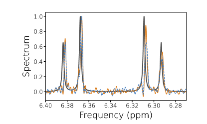
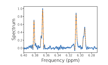
In this work, we fill the gap and provide insight into the noise tolerance of the digital quantum simulations of NMR experiments with NISQ devices. To this end, we present the simulation of NMR spectroscopy of small organic molecules on publicly available quantum processors, such as IBM’s quantum processors based on superconducting qubits and IonQ’s Aria trapped ion quantum computer available via Amazon Bracket, as it is showcased in Fig. 1 for NMR spectrum of cis-3-chloroacrylic acid. The simulation on quantum computers nicely reproduce the known spectrum. However, even for such a small molecule [see Eq. (2)], we observe the signatures of noise as slight deviations from the predicated resonances. This motivates further investigation of the impact of noise on quantum simulation of NMR spectroscopy, which is the main objective of the present work. In the actual NMR experiments, the nuclear spins unavoidably interact with their environment, which is similar to the noise acting on qubits. Therefore simulation of NMR spectra on quantum computers can endure a certain amount of noise. We quantify this amount of noise and try to find a threshold for the noise that can be tolerated.
II The Spin Hamiltonian
The NMR problem involves the interaction of the nuclear spins of molecules with an external magnetic field. To tackle such a problem, we first express the molecules of interest in terms of spin- models that can be naturally mapped to qubits. In the presence of a static magnetic field , the spin Hamiltonian of a given molecule in the liquid phase reads
| (1) |
where is the gyromagnetic ratio, the total number of spins, encodes the chemical shifts caused by electrons shielding the magnetic field, represents the nuclear spin, and determines the strength of the interaction between -th and -th nuclear spins. Note that in the liquid phase, the Hamiltonian has the SU(2) symmetry. The chemical shifts and the spin–spin couplings are obtained through quantum chemical calculations (e.g., DFT calculations), similarly to the approach outlined in Refs. [36, 37, 38, 39].
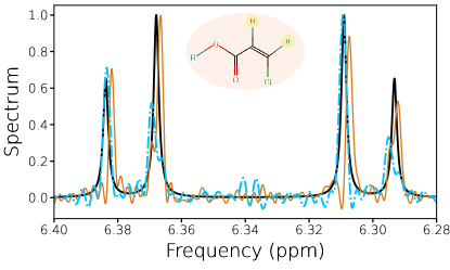
In the present work, we focus on 1H NMR spectroscopy of two molecules, namely cis-3-chloroacrylic acid (), and 1,2,4-trichlorobenzene (). Both molecules have three spin- nuclei (protons). However, due to the rapid exchange of the acidic proton in the solvent , the carboxylic signal is usually omitted. Therefore, the cis-3-chloroacrylic acid is characterized by the following chemical shifts (in units of ppm) and spin-spin interaction (in Hz)
| (2) |
The Hamiltonian of 1,2,4-trichlorobenzene () is described by
| (3) | |||
| (4) |
The chemical shifts and the spin-spin couplings were determined to fit the experimental spectrum [40]. In addition, for 1,2,4-trichlorobenzene, the spin-spin couplings for the two opposing protons were taken from [41].
III Method
In a 1D NMR experiment, an oscillatory external probe () is applied perpendicular to the static magnetic field mentioned above. From now on, we assume that the static magnetic field () is applied in the direction and the oscillatory one in the direction. Such a probe polarizes the nuclear spins and induces a time-dependent magnetic moment, that within linear response theory (linear order response in ), has the form
| (5) |
where is the correlation function that can be formulated as
| (6) |
where is the total nuclear spin that evolves in time as
| (7) |
and is the initial equilibrium density matrix (in the absence of the probe). As the temperature is quite large in the NMR experiment, compared to all energy scales in Eq. (1), we assume that all initial states are equally probable, resulting in a density operator of the form .
The NMR spectrum is measured based on the molecule absorption, which in turn reveals the internal structure of the molecule. The NMR spectrum is defined as
| (8) |
where is the effective decoherence rate that physically arises due to the interaction of nuclear spin with its environment.
In order to find an algorithm for obtaining such a correlation function on a quantum processor, we consider a Trotterized time evolution [42, 43], where the the Hamiltonian of the NMR problem is written in the sum of partial Hamiltonians and the time evolution is implemented according to the Trotterization formula
| (9) |
with being the Trotter-step size and the approximation is controlled by the size of and [43]. For the NMR problem, the terms correspond to the onsite energy terms and the interaction terms between spins. The time propagation under a partial Hamiltonian can be implemented on the quantum computer directly, using the unitary gates on the quantum computer.
| (10) |
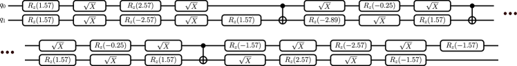
Figure 2 illustrates the quantum circuit corresponding to the Trotterized time evolution of the Hamiltonian in Eq. (2).
In a Trotterized time evolution, the Trotter time step should be, on the one hand, small enough to minimize the Trotter error and adequately cover the entire spectrum of the molecule. On the other hand, the step size must be large enough to reduce the total number of Trotter steps required. In this respect, it is advantageous to perform the unitary transformation that transforms the total magnetization in -direction as
| (11) |
Consequently, the Fourier transform of becomes
| (12) |
Furthermore, by introducing the eigenstates of as following,
| (13) |
the response functions can be rewritten according to
| (14) |
with [44, 28]. Note the sum can be restricted to positive initial magnetization due to the symmetry of the Hamiltonian (which can be seen for example by flipping all spins around their X-axes, which changes , but keeps the Hamiltonian unchanged). In order to evaluate each term in the summation, we can initialize the qubits in a configuration leading to , and perform a Trotterized time evolution to obtain .
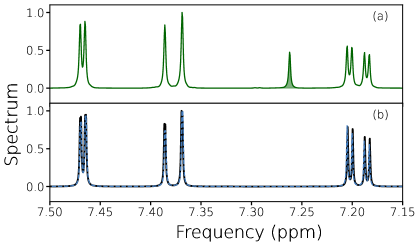
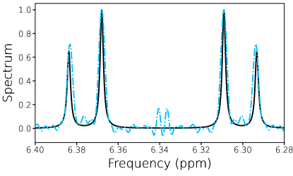
In order to verify the outlined algorithm, we use a noise-free simulator to obtain the NMR spectrum of 1,2,4-trichlorobenzene () molecule and we compare it to the known experimental results [40]. We choose the decoherence rate , see Eq. (8), such that the simulated broadening of the peaks matches approximately the experimental broadening. As is shown in Fig. 3, the simulated results agree very well with the experimental data, apart from the marked peak that is known to be caused by the solvent in which the sample is embedded.
IV Results on NISQ devices
In the following section, we present the outcome of executing the aforementioned method for organic molecules on quantum computing platforms. In the 1D NMR experiment, the NMR response is measured at sufficiently long times after the applied oscillatory magnetic field, such that the spin dynamics reach a steady state, in which the average magnetization is zero. However, in the performed simulation on current quantum computing platforms, we were restricted with regard to the total number of the circuits, i.e., the number of Trotter steps for the time evolution. We have observed that such a maximum number of Trotter steps is smaller than the spin relaxation times, and hence the oscillations in the averaged magnetization did not necessarily vanish at the end of the simulation, see Appendix A. Such a restriction also poses a maximum frequency grid for the spectrum. In order to be able to obtain the spectrum more finely, we have added additional zeros in the averaged magnetization, as is discussed in Appendix A.
The spectrum of cis-3-chloroacrylic acid is symmetric around the center of the rotating frame, which is a manifestation of the symmetry of the interaction matrix of any two spin systems. In general, the asymmetric part of the spectral function originates from the total magnetization in the direction, see Eq. (12), which in the case of 2 spins vanishes. In particular, the contributions from various spins should cancel each other. However such a cancellation does not occur in the simulation results as noise manifests itself in disordered terms in the effective Hamiltonian being simulated on a noisy device, see Ref. [45]. In fact, if we impose such a symmetry, and neglect the second contribution to Eq. (12), we can significantly improve the results particularly for the IonQ device, see Appendix B.
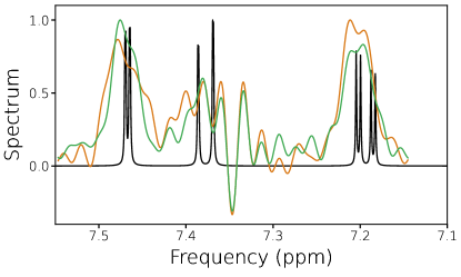
Fig. 4 depicts the spectrum of 1,2,4-trichlorobenzene simulated using the IBM Perth devise on two different days. As illustrated, the impact of noise on the simulations is so significant that we cannot reproduce all the fine structures of the eaxct NMR spectrum. This is due to the fact that the Hamiltonian of 1,2,4-trichlorobenzene has three spins with all-to-all interactions, see Eq. (4), On the IBM-Q device, we selected a three-qubit chain to execute the algorithm. Due to the Hamiltonian’s all-to-all interaction, it is necessary to swap the positions of the qubits. For simulating NMR spectra of 1,2,4-trichlorobenzene, we employed a second-order Trotter expansion. This approach results in application of 15 CNOT gates during each Trotter step. Moreover, due to this large-depth circuit, we have picked a smaller number of Trotter steps. This number is far below the required time for the average magnetization to reach zero, and hence the added zeros (see the above paragraph) cause an abrupt change in the magnetization. This, in turn, results in the oscillations around the center of the rotating frame.
V Noise analysis
In this section, we analyze the impact of noise on the obtained NMR spectrum and construct a noise model which can reproduce most of the features of the shown results from the IBM quantum processors. We also define an effective decoherence rate that quantifies the amount of noise in a circuit, and the limitations it implies to the accuracy of the resulting spectrum.
V.1 Error sources
Disentangling the qubits from their embedded environments is one of the most challenging task of the realizations of quantum processors. At the same time modeling the noise that occurs in the quantum chips is quite complex. Typically each single qubit is characterized by the parameters and [46, 47]. The former is the damping time scale, i.e., the time scale after which a qubit in an excited state will decay to its ground state. The second time scale is pure dephasing time, which refers to the time scale, after which the qubit’s phase is lost (when removing the contribution from damping). Another source of error, apart from the imperfections of the qubits, is the erroneous unitary operation implemented by the gate. Such coherent error can be interpreted as effective additional unitary gate. Additionally, leakage out of the computational basis of the qubit [48], and a fast return back to mentioned basis may be mapped to incoherent errors.
V.2 Discrete noise model in quantum circuits
In order to account for the incoherent errors, Lindbladian master equations are used routinely. In this approach, the density operator of the qubits is described by the Lindblad master equation
| (15) |
where the Hamiltonian describes coherent evolution of the qubits (the effect of gates) and the terms on the second line describe the incoherent noise. Here, qubit damping corresponds to operator with a rate of , and qubit pure dephasing corresponds to with a rate of . Additionally, qubit depolarising noise corresponds to the summation over the three Pauli operators with factors .
The Lindblad superoperator also describes incoherent gate errors on the level of quantum circuits [31, 49]. Here, each ideal gate is replaced by a gate-noise superoperators , where
| (16) |
and is the gate time. The form of the noise Lindbladian may be modified because it represents the effect of incoherent noise acting during the implementation of the gate. In particular, while the gates corresponding to small-angle rotations will keep the nature of the noise intact, the large-angle rotations will drastically modify the form of the noise, usually leading to a form close to depolarizing noise [49].
In our modeling of IBM’s quantum computing devices, we model the gate errors as depolarizing noise as all the native gates are corresponding to large angle rotations (except the which is a virtual gate). This model is consistent with noise spectroscopy performed on the IBM devices [50]. To fix the used strength of the depolarising noise after each gate, we use the universal connection between incoherent noise and gate fidelity [51], which yields
| (17) |
where is the number of qubits the gate is acting on, and is the dimension of the space. The values for are obtained from IBM calibration data. We also account for the inherent noise during the qubit idling, i.e., considering damping and dephasing of qubits that are not involved in a two-qubit gates.
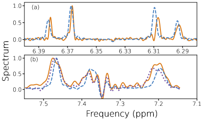
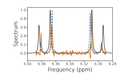
Figure 5(a) illustrates the comparison of the simulation which includes only depolarising noise according to Eq. (17) with the IBM results for cis-3-chloroacrylic acid. As it is shown the agreement is rather good. The peak positions show slight differences and also vary between different runs (see Appendix D), which is a manifestation of the effect of quasistatic coherent errors. Also the peak widths can vary between different runs.
Figure 5(b) shows the comparison of the simulation which includes only depolarising noise (blue dashed lines) with the IBM results for the case of 1,2,4-trichlorobenzene. This system involves more interaction terms and hence more gates in the circuit for time evolution [in total 15 CNOTs per Trotter step, in comparison to 3 CNOTs in case (a)]. As we see, here the broadenings of the peaks are not well reproduced by the simulation with including only depolarising noise. This difference is due to coherent errors, as demonstrated in the second numerical simulation (dotted lines), where we include coherent errors by applying an additional and on each involved gate-type determined by a fitting routine. We use angles whose magnitudes are consistent with the noise spectroscopy of Ref. [50] and correspond to gate errors that are smaller than given in the calibration data. (The size of the incoherent errors were kept unchanged). As illustrated, with the proper choice of angles corresponding to coherent errors, we are able to reproduce the main features of the simulated spectrum on IBM. This demonstrates that also coherent errors can effectively broaden the spectrum in large-depth circuits.
V.3 Effective decoherence rate
Having constructed an effective noise model, in this section we aim to define an effective decoherence rate that quantifies the amount of noise in a circuit, and the limitations it implies to the accuracy of the resulting spectrum. The noise during the quantum computation corresponds to the simulation of an effective open quantum system [52]. Motivated by this, we define the effective decoherence rate as
| (18) |
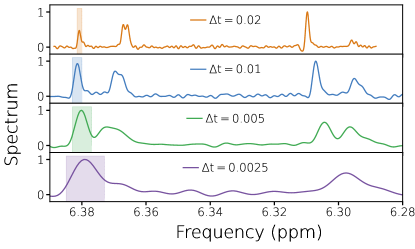
with the summation performed over all gates applied at one Trotter circuit (including identity gates), being the simulated (Trotter) time step, error of the -th applied gate, and the number of spins. It is important to note that the effective decoherence rate is inversely proportional to the Trotter step size [31]. This rate is expected to describe the error in the simulated energy-levels of the system and therefore also the broadening of peaks in the simulated spectra. To verify this hypothesis, we look at the simulated NMR spectrum on the IBMQ cloud for various Trotter steps. As is shown in Fig. 6, the broadening of the peaks in the simulated spectrum is in good agreement with the estimated effective broadenings, illustrated for various trotter steps. This indicates that indeed the impact of noise is less pronounced at larger trotter steps. However, there is an upper bound on the choice of the maximum Trotter step in order to keep the Trotterization errors small. The Trotter error is detectable in the simulation for (see Appendix C).
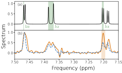
Such an effective decoherence rate allows us to quantify the precision with which we can simulate the NMR spectrum on NISQ devices. In particular, in the case of 1,2,4-trichlorobenzene, see Figs. 4 and 5, the effective decoherence rate is much larger than the spin-spin coupling between spin 2 and 3 , see Fig. 7(a). Consequently, we cannot resolve the energy splitting caused by interactions. We can therefore (in principle) neglect the terms in the Hamiltonian Eq. (4). Neglecting the coupling simplifies 1,2,4-trichlorobenzene to a nearest neighbor Hamiltonian. In the first-order Trotter expansion, each Trotter circuit then contains 6 CNOT gates (instead of 15 CNOTs). As a result, the simulated NMR spectrum of the reduced Hamiltonian is significantly improved, as can be seen by comparing Fig. 5 with Fig. 7. For completeness, we have also presented the simulation with depolarising noise, and we see that the resulting spectrum agrees well with the simulated one on IBMQ cloud.
VI Conclusion
We demonstrated the digital quantum simulation of NMR experiments, employing publicly available quantum processors. We compared the results against conventional methods to study the effect of noise. We provided a noise model that can accurately reproduce the main features of the obtained spectra. We formulated an effective decoherence rate, based on the noise parametrization of the quantum devices, which can define the energy scale up to which we can accurately simulate NMR spectra with a given NISQ device. Moreover, we showcase how such an effective decoherence rate provides insight into tailoring the circuit to a smaller depth, and, in turn, improve the obtained NMR spectra.
In this work, we could only show the simulation of NMR spectra for very small organic molecules due to present limitations of NISQ devices. However we witness a surge of quantum computing platforms that continue to proliferate with ever increasing qubit gate fidelities. With the increase of the quantity and quality of quantum computers, it remains quite relevant to find interesting applications. In this respect, our results highlight a promising application for publicly available quantum computers, as well as showcasing how one can tailor the quantum algorithms through noise analysis, paving the way for better employing quantum tasks on NISQ devices.
Acknowledgements.
This work was supported by the German Federal Ministry of Education and Research, through projects QSolid (13N16155) and Q-Exa (13N16065). We also want to thank Peter Pinski, Sonia Alvarez, and Julius Kleine Büning for insightful input and fruitful discussions.References
- Kjaergaard et al. [2020] M. Kjaergaard, M. E. Schwartz, J. Braumüller, P. Krantz, J. I.-J. Wang, S. Gustavsson, and W. D. Oliver, Annual Review of Condensed Matter Physics 11, 369 (2020).
- Krantz et al. [2019] P. Krantz, M. Kjaergaard, F. Yan, T. P. Orlando, S. Gustavsson, and W. D. Oliver, Applied Physics Reviews 6, 021318 (2019), https://pubs.aip.org/aip/apr/article-pdf/doi/10.1063/1.5089550/16667201/021318_1_online.pdf .
- Wendin [2017] G. Wendin, Reports on Progress in Physics 80, 106001 (2017).
- Noiri et al. [2022] A. Noiri, K. Takeda, T. Nakajima, T. Kobayashi, A. Sammak, G. Scappucci, and S. Tarucha, Nature 601, 338 (2022).
- Flamini et al. [2018] F. Flamini, N. Spagnolo, and F. Sciarrino, Reports on Progress in Physics 82, 016001 (2018).
- Henriet et al. [2020] L. Henriet, L. Beguin, A. Signoles, T. Lahaye, A. Browaeys, G.-O. Reymond, and C. Jurczak, Quantum 4, 327 (2020).
- Lanyon et al. [2011] B. P. Lanyon, C. Hempel, D. Nigg, M. Müller, R. Gerritsma, F. Zähringer, P. Schindler, J. T. Barreiro, M. Rambach, G. Kirchmair, M. Hennrich, P. Zoller, R. Blatt, and C. F. Roos, Science 334, 57 (2011).
- Bruzewicz et al. [2019] C. D. Bruzewicz, J. Chiaverini, R. McConnell, and J. M. Sage, Applied Physics Reviews 6, 021314 (2019).
- Gambetta et al. [2012] J. M. Gambetta, A. D. Córcoles, S. T. Merkel, B. R. Johnson, J. A. Smolin, J. M. Chow, C. A. Ryan, C. Rigetti, S. Poletto, T. A. Ohki, M. B. Ketchen, and M. Steffen, Phys. Rev. Lett. 109, 240504 (2012).
- Kueng et al. [2016] R. Kueng, D. M. Long, A. C. Doherty, and S. T. Flammia, Phys. Rev. Lett. 117, 170502 (2016).
- Preskill [2018] J. Preskill, Quantum 2, 79 (2018).
- Maciejewski et al. [2020] F. B. Maciejewski, Z. Zimborás, and M. Oszmaniec, Quantum 4, 257 (2020).
- Temme et al. [2017] K. Temme, S. Bravyi, and J. M. Gambetta, Phys. Rev. Lett. 119, 180509 (2017).
- Montanaro [2016] A. Montanaro, npj Quantum Information 2, 15023 (2016).
- Shor [1994] P. Shor (1994) pp. 124–134.
- Shor [1997] P. W. Shor, SIAM Journal on Computing 26, 1484 (1997).
- Fauseweh [2024] B. Fauseweh, Nature Communications 15, 2123 (2024).
- O’Malley et al. [2016] P. J. J. O’Malley, R. Babbush, I. D. Kivlichan, J. Romero, J. R. McClean, R. Barends, J. Kelly, P. Roushan, A. Tranter, N. Ding, B. Campbell, Y. Chen, Z. Chen, B. Chiaro, A. Dunsworth, A. G. Fowler, E. Jeffrey, E. Lucero, A. Megrant, J. Y. Mutus, M. Neeley, C. Neill, C. Quintana, D. Sank, A. Vainsencher, J. Wenner, T. C. White, P. V. Coveney, P. J. Love, H. Neven, A. Aspuru-Guzik, and J. M. Martinis, Phys. Rev. X 6, 031007 (2016).
- Kandala et al. [2017] A. Kandala, A. Mezzacapo, K. Temme, M. Takita, M. Brink, J. M. Chow, and J. M. Gambetta, Nature 549, 242 (2017).
- Monroe et al. [2021] C. Monroe, W. C. Campbell, L.-M. Duan, Z.-X. Gong, A. V. Gorshkov, P. W. Hess, R. Islam, K. Kim, N. M. Linke, G. Pagano, P. Richerme, C. Senko, and N. Y. Yao, Rev. Mod. Phys. 93, 025001 (2021).
- Zhang et al. [2017] J. Zhang, G. Pagano, P. W. Hess, A. Kyprianidis, P. Becker, H. Kaplan, A. V. Gorshkov, Z.-X. Gong, and C. Monroe, Nature 551, 601 (2017).
- Cerezo et al. [2021a] M. Cerezo, A. Arrasmith, R. Babbush, S. C. Benjamin, S. Endo, K. Fujii, J. R. McClean, K. Mitarai, X. Yuan, L. Cincio, and P. J. Coles, Nature Reviews Physics 3, 625 (2021a).
- Liu et al. [2023] J. Liu, F. Wilde, A. A. Mele, L. Jiang, and J. Eisert, “Stochastic noise can be helpful for variational quantum algorithms,” (2023), arXiv:2210.06723 [quant-ph] .
- Cerezo et al. [2021b] M. Cerezo, A. Sone, T. Volkoff, L. Cincio, and P. J. Coles, Nature Communications 12, 1791 (2021b).
- Fauseweh and Zhu [2021] B. Fauseweh and J.-X. Zhu, Quantum Information Processing 20, 138 (2021).
- Salathé et al. [2015] Y. Salathé, M. Mondal, M. Oppliger, J. Heinsoo, P. Kurpiers, A. Potočnik, A. Mezzacapo, U. Las Heras, L. Lamata, E. Solano, S. Filipp, and A. Wallraff, Phys. Rev. X 5, 021027 (2015).
- Barends et al. [2015] R. Barends, L. Lamata, J. Kelly, L. García-Álvarez, A. G. Fowler, A. Megrant, E. Jeffrey, T. C. White, D. Sank, J. Y. Mutus, B. Campbell, Y. Chen, Z. Chen, B. Chiaro, A. Dunsworth, I.-C. Hoi, C. Neill, P. J. J. O’Malley, C. Quintana, P. Roushan, A. Vainsencher, J. Wenner, E. Solano, and J. M. Martinis, Nature Communications 6, 7654 (2015).
- Sels et al. [2020] D. Sels, H. Dashti, S. Mora, O. Demler, and E. Demler, Nature Machine Intelligence 2, 396 (2020).
- Seetharam et al. [2023a] K. Seetharam, D. Biswas, C. Noel, A. Risinger, D. Zhu, O. Katz, S. Chattopadhyay, M. Cetina, C. Monroe, E. Demler, and D. Sels, Science Advances 9, eadh2594 (2023a).
- Lloyd [1996] S. Lloyd, Science 273, 1073 (1996).
- Fratus et al. [2023a] K. R. Fratus, K. Bark, N. Vogt, J. Leppäkangas, S. Zanker, M. Marthaler, and J.-M. Reiner, “Describing trotterized time evolutions on noisy quantum computers via static effective lindbladians,” (2023a), arXiv:2210.11371 [quant-ph] .
- Blümich and Singh [2018] B. Blümich and K. Singh, Angewandte Chemie International Edition 57, 6996 (2018).
- Reif et al. [2021] B. Reif, S. E. Ashbrook, L. Emsley, and M. Hong, Nature Reviews Methods Primers 1, 2 (2021).
- Emwas et al. [2020] A.-H. Emwas, K. Szczepski, B. G. Poulson, K. Chandra, R. T. McKay, M. Dhahri, F. Alahmari, L. Jaremko, J. I. Lachowicz, and M. Jaremko, Molecules 25 (2020), 10.3390/molecules25204597.
- Wishart et al. [2022] D. S. Wishart, L. L. Cheng, V. Copié, A. S. Edison, H. R. Eghbalnia, J. C. Hoch, G. J. Gouveia, W. Pathmasiri, R. Powers, T. B. Schock, L. W. Sumner, and M. Uchimiya, Metabolites 12 (2022), 10.3390/metabo12080678.
- Grimme et al. [2017] S. Grimme, C. Bannwarth, S. Dohm, A. Hansen, J. Pisarek, P. Pracht, J. Seibert, and F. Neese, Angewandte Chemie International Edition 56, 14763 (2017).
- Yesiltepe et al. [2018] Y. Yesiltepe, J. R. Nuñez, S. M. Colby, D. G. Thomas, M. I. Borkum, P. N. Reardon, N. M. Washton, T. O. Metz, J. G. Teeguarden, N. Govind, and R. S. Renslow, Journal of Cheminformatics 10, 52 (2018).
- Willoughby et al. [2014] P. H. Willoughby, M. J. Jansma, and T. R. Hoye, Nature Protocols 9, 643 (2014).
- Jonas et al. [2022] E. Jonas, S. Kuhn, and N. Schlörer, Magnetic Resonance in Chemistry 60, 1021 (2022).
- Hoch et al. [2023] J. C. Hoch, K. Baskaran, H. Burr, J. Chin, H. R. Eghbalnia, T. Fujiwara, M. R. Gryk, T. Iwata, C. Kojima, G. Kurisu, D. Maziuk, Y. Miyanoiri, J. R. Wedell, C. Wilburn, H. Yao, and Y. Masashi, Nucleic Acids Research 51, 150504 (2023).
- Dischler [1966] B. Dischler, Angewandte Chemie International Edition in English 5, 623 (1966).
- Trotter [1959] H. F. Trotter, Proceedings of the American Mathematical Society 10, 545 (1959), full publication date: Aug., 1959.
- Childs et al. [2021] A. M. Childs, Y. Su, M. C. Tran, N. Wiebe, and S. Zhu, PRX Quantum 11, 011020 (2021).
- Seetharam et al. [2023b] K. Seetharam, D. Biswas, C. Noel, A. Risinger, D. Zhu, O. Katz, S. Chattopadhyay, M. Cetina, C. Monroe, E. Demler, and D. Sels, Science Advances 9 (2023b), 10.1126/sciadv.adh2594.
- Reiner et al. [2018] J.-M. Reiner, S. Zanker, I. Schwenk, J. Leppäkangas, F. Wilhelm-Mauch, G. Schön, and M. Marthaler, Quantum Science and Technology 3, 045008 (2018).
- Klimov et al. [2018] P. Klimov, J. Kelly, Z. Chen, M. Neeley, A. Megrant, B. Burkett, R. Barends, K. Arya, B. Chiaro, Y. Chen, A. Dunsworth, A. Fowler, B. Foxen, C. Gidney, M. Giustina, R. Graff, T. Huang, E. Jeffrey, E. Lucero, J. Mutus, O. Naaman, C. Neill, C. Quintana, P. Roushan, D. Sank, A. Vainsencher, J. Wenner, T. White, S. Boixo, R. Babbush, V. Smelyanskiy, H. Neven, and J. Martinis, Physical Review Letters 121, 090502 (2018).
- Schlör et al. [2019] S. Schlör, J. Lisenfeld, C. Müller, A. Bilmes, A. Schneider, D. P. Pappas, A. V. Ustinov, and M. Weides, Physical Review Letters 123, 190502 (2019).
- Chen et al. [2016] Z. Chen, J. Kelly, C. Quintana, R. Barends, B. Campbell, Y. Chen, B. Chiaro, A. Dunsworth, A. Fowler, E. Lucero, E. Jeffrey, A. Megrant, J. Mutus, M. Neeley, C. Neill, P. O’Malley, P. Roushan, D. Sank, A. Vainsencher, J. Wenner, T. White, A. Korotkov, and J. M. Martinis, Physical Review Letters 116 (2016), 10.1103/physrevlett.116.020501.
- Fratus et al. [2023b] K. R. Fratus, J. Leppäkangas, M. Marthaler, and J.-M. Reiner, “The discrete noise approximation in quantum circuits,” (2023b), arXiv:2311.00135 [quant-ph] .
- Stadler et al. [2024] P. Stadler, M. Lodi, A. Khedri, R. Reiner, K. Bark, N. Vogt, M. Marthaler, and J. Leppäkangas, “Demonstration of system-bath physics on gate-based quantum computer,” (2024), arXiv:2404 .
- Abad et al. [2022] T. Abad, J. Fernández-Pendás, A. Frisk Kockum, and G. Johansson, Phys. Rev. Lett. 129, 150504 (2022).
- Fratus et al. [2022] K. R. Fratus, K. Bark, N. Vogt, J. Leppäkangas, S. Zanker, M. Marthaler, and J.-M. Reiner, “Describing trotterized time evolutions on noisy quantum computers via static effective lindbladians,” (2022), arXiv:2210.11371 [quant-ph] .
Appendix A Time evolution of Magnetization
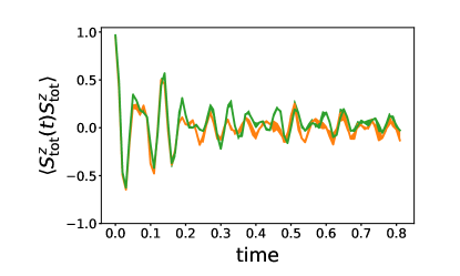
In this appendix we look at the time evolution of the correlation function simulated on IBM quantum computing platforms. Fig. 8 depicts the correlation function as a function of time, indicating the decay of correlation function with time. In the NMR experiment the spectrum is measured at sufficiently long times after the application of the magnetic field such that the system reaches a state in which average magnetization vanishes and hence the correlation function. As is shown in Fig. 8 there remain some small oscillations around zero at long times due to the limitation of number of Trotter steps. As the spectrum is obtained via the Fourier transform of the correlation function, see Eq. (12), the frequency interval is inversely proportional to the number of Trotter steps. Thereby we added additional zeros to the correlation functions in order to be able to obtain the spectrum on a finer frequency grid. Fig. 9 presents the comparison of the spectrum with and without adding such additional zeros for one of the simulations on IBM’s devices.
Appendix B The symmetrized NMR spectra
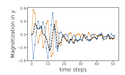
In this appendix, we discuss the symmetry breaking that occurs in the simulations as an artifact of noise of NISQ devices. In particular in Fig. 10, we present the magnetization in direction simulated on IonQ’s Aria. Note that due to the symmetry of the Hamiltonian of cis-3-chloroacrylic acid, see Eq. 2, we expect , such that the total magnetization in the direction vanishes. However, due to the presence of noise, such a symmetry is numerically broken. This is a manifestation of coherent errors [45] resulting in additional disordered effective Hamiltonian terms that break the mentioned symmetry. In particular, in additional numerical simulations we find that the spectroscopy on quantum computer is especially fragile against Hamiltonian disorder terms .
Appendix C The trotter error
For a Trotterized time evolution, it is advantageous to increase the trotter step size to be able to simulate longer times, and also to decrease the impact of noise, as discussed in Sec. V.3. However, by increasing the Trotter step size, we get an error from the Trotterization of the time evolution. Fig. 12 depicts the occurrence of such an error in the form of shifts of the resonances. Note that in the simulation with an on-gate depolarizing noise, we can reproduce such shifts to the actual resonances.
Appendix D Additional results
In this appendix, we present further simulations of the NMR spectrum of cis-3-chloroacrylic acid on IBM’s processors. It is interesting to note that the deviations of the predicted resonances from the exact result varies in simulations performed on different days, which can be a manifestation of quasistatic coherent noise.