Neural network prediction of model parameters for strong lensing samples from Hyper Suprime-Cam Survey

Abstract

Galaxies that cause the strong gravitational lensing of background galaxies provide us crucial information about the distribution of matter around them. Traditional modelling methods that analyse such strong lenses are both time and resource consuming, require sophisticated lensing codes and modelling expertise. To study the large lens population expected from imaging surveys such as LSST, we need fast and automated analysis methods. In this work, we build and train a simple convolutional neural network with an aim to rapidly predict model parameters of gravitational lenses. We focus on the most important lens mass model parameters, namely, the Einstein radius, the axis ratio and the position angle of the major axis of the mass distribution. The network is trained on a variety of simulated data with an increasing degree of realism and shows satisfactory performance on simulated test data. The trained network is then applied to the real sample of galaxy-scale candidate lenses from the Subaru HSC, a precursor survey to LSST. Unlike the simulated lenses, we do not have the ground truth for the real lenses. Therefore, we have compared our predictions with those from YattaLens , a lens modelling pipeline. Additionally, we also compare the parameter predictions for 10 HSC lenses that were also studied by other conventional modelling methods. These comparisons show a fair quantitative agreement on the Einstein radius, although the axis ratio and the position angle from the network as well as the individual modelling methods, seem to have systematic uncertainties beyond the quoted errors.

1 Introduction

Gravitational lensing can result in the formation of multiple images of sources which are sufficiently well aligned with a lensing potential. Observing and analysing such strong gravitational lensing effects, for example, the distortions of the background sources, the positions and magnifications of the multiple images, and the time delays in the case of transient sources, can provide us crucial information about the properties of the lens and the source. Strong lenses can be studied to probe the mass distribution in galaxies (e.g., Koopmans et al., 2006; Auger et al., 2010; Sonnenfeld et al., 2015; Shajib et al., 2021) and in groups and clusters (e.g., Limousin et al., 2009; More et al., 2012; Oguri et al., 2012; Newman et al., 2013; Allingham et al., 2023).

Lens systems have been searched in ongoing imaging surveys such as the Hyper Suprime-Cam (HSC) survey through campaigns such as the Survey of Gravitationally-lensed Objects in HSC Imaging (SuGOHI). This has resulted in the discovery of hundreds of strong gravitational lens candidates in various categories using different search algorithms (see table 1 in Jaelani et al., 2023). Lens systems have also been searched in the Dark Energy survey via a variety of techniques (e.g., Nord et al., 2020; Rojas et al., 2022). The number of discovered gravitational lens systems is going to increase by an order of magnitude with the next generation ground based imaging surveys such as the Vera Rubin Observatory’s Legacy Survey of Space and Time (LSST). Lens modelling techniques (e.g., Nightingale et al., 2021) are used to estimate the parameters that describe the mass distribution in such individual lens systems. Lens modelling is in general time and resource consuming, often requires individual attention, in addition to sophisticated lens modelling codes. Some of the steps that require human attention are identifying lensed features, masking out foreground contaminants, and finding an adequate initial guess for the lens model parameters. Finding more efficient ways to study gravitational lenses is the need of the hour given the large amount of data which will be available imminently.

On the other hand, the era of large scale computing has already begun. Machine Learning (ML) has emerged as a revolutionary tool in order to mine data and identify features or various characteristics of the data (e.g., Moriwaki et al., 2023). The automation implies faster analysis results. ML techniques such as neural networks are a very effective way in performing tasks like image classifications and parameter estimations. A neural network can be trained to analyse images of gravitationally lensed systems, for purposes like finding out strong lenses (e.g., Jacobs et al., 2017; Rojas et al., 2022) and estimating lensing parameters (e.g., Hezaveh et al., 2017; Schuldt et al., 2023; Gentile et al., 2023). A neural network once trained, can predict the parameters just by analysing the features in the image such as shape, image separation and brightness. A neural network can statistically infer the parameters of commonly used lensed models, with accuracy comparable to these sophisticated methods but about ten million times faster (Hezaveh et al., 2017). Once we infer the lens parameters statistically, we can use them to probe various dark matter properties, for instance, the mass fraction (Oguri et al., 2014) and mass distribution (e.g., More et al., 2012). ML approach may not lead to accurate measurements on individual lens systems but can provide reasonable estimates for the distribution of lens parameters in a statistical manner.

Hezaveh et al. (2017) demonstrated that they could use Convolutional Neural Network (CNNs) to infer the lens model parameters, in particular, the Einstein radius. Furthermore, Levasseur et al. (2017) have applied a Bayesian framework to determine the uncertainties in the lens parameters. These studies have mainly considered images of strong lenses at high spatial resolution, for instance, with image quality similar to that of the Hubble Space Telescope.

However, a significant fraction of strong lens systems in the near future will be obtained from the images taken by ground based telescopes, where we will have to deal with unique challenges including poorer image quality due to atmospheric seeing and the lower pixel resolution. To address this, we have designed a CNN that enables us to analyse the images of lens systems taken from ground based telescope surveys. In particular we focus on the HSC survey given the existence of data, a sample of known lenses from the survey, and its similarity in terms of depth and image quality to the Rubin LSST. We train our CNN on a simulated sample of HSC-like lenses and test it on the simulated as well as real grade A and B SuGOHI lenses to infer lens mass model parameters like the Einstein radius, the axis ratio and the position angle of the major axis of the lens mass distribution. We process the SuGOHI lenses before feeding them to the network using a pipeline called YattaLens (YL, Sonnenfeld et al., 2018) in order to subtract the lens light and infer the lens model parameters to obtain the benchmarks for our study. While this work was in progress, we became aware of Schuldt et al. (2023), who designed a ResNet in order to infer the lens model parameters. While there are similarities between the two approaches, there are also differences in terms of the choice of the network, the suite of training simulations and their weights, the test samples as well as the comparisons, even though we reach similar conclusions. In addition, we also systematically analyze the reasons for various failure modes. We compare our results with the inferences from traditional modeling carried out in Sonnenfeld et al. (2019, henceforth, referred to as S19) and in Schuldt et al. (2023, henceforth, referred to as S23) for a sample of 10 grade A SuGOHI lenses.

This paper aims towards modelling the strong lenses obtained from ground based surveys like the HSC using ML techniques such as CNNs and is structured as follows. In the Section 2, we discuss the construction of simulated and real datasets that were used to train and test our CNN. Section 3 describes the architecture of our CNN and the training process in detail. In the Section 4 we discuss our results and we conclude with a summary in Section 5.

2 Construction of training data

The performance of any machine learning architecture is crucially dependent on the realism and representative nature on which the machine is trained. In this section, we describe the generation of the training and test data used to train and validate the network, respectively. We also present details of the real lens samples from SuGOHI, including the pre-processing we performed before we used them as a test sample.

2.1 Simulated datasets

Gravitational lensing is a complex inverse problem. The inference of the parameters of the lens model has to be performed with the help of a noisy manifestation of the lensed source, where the true shape of the source is not known. Depending upon the unknown location of the source with respect to the lens as well as the lensing potential, the lensed images can take a variety of configurations. Therefore the CNN has to be trained on a large number of lensed images. The number of known galaxy-scale lenses from the HSC Survey are in $\mathcal{O}(100)$. Therefore, we generate a large number of lensed systems in order to train our network. We generate a sample of simulated lens systems using SIMCT (More et al., 2016), a framework which allows for lensed images to be generated for a corresponding survey. We use SIMCT to generate a final lensed image sample with properties that are matched to the HSC Survey depth, seeing and pixel resolution. While the detailed framework for SIMCT is given in More et al. (2016), we briefly summarise the methodology of producing lens sample for completeness.

The SIMCT pipeline generates lens samples via a hybrid approach where lensed features are model images superposed on real image cutouts of potential lensing galaxies with actual line-of-sight objects. The background source such as a galaxy or a quasar is defined with a parametric model and the parameter values come from realistic distributions of luminosity functions, redshifts, sizes and colors. The lens mass model is defined by taking the light properties such as the magnitudes, redshifts, ellipticity and position angle of the potential lensing galaxy and converting them into the parameters of a typical lens density profile such as the Singular Isothermal Ellipsoid (SIE) under the assumption that mass follows light and via standard scaling relations. External shear is drawn from a uniform distribution. Only those galaxies with sufficient lensing probabilities and lensed images that are detectable, in a given survey data, comprise the final lens sample.

The simulated lensed arcs used in this work come from the same sample as that used in Jaelani et al. (2023). Thus, the reader is referred to the Section 3 of Jaelani et al. (2023) for the specific settings, the scaling relations and the distributions used to produce this sample. We note that we have added Posson noise to the simulated model arcs after convolving with the coadded PSF from the HSC database available at the location of central lens galaxy in each of the g, r and i bands.

We construct numerous training samples, successively, by adding various degrees of realism to our simulated arcs. These exploratory training samples were labelled as the following cases: a) Simulated arcs (PSF-convolved and Poisson noise added) without any background noise, b) Simulated arcs, as before, but with Gaussian background noise, c) Simulated arcs (same as in sample a) added to the image cutout of the respective HSC galaxy (central lens galaxy used to model the arcs, see Appendix B), d) Same as sample c but processed by YL to subtract out the light profile of the central galaxy. The networks trained on all these training samples do not produce satisfactory results (see Section 4) but are described here for completeness.

Lastly, we describe below the final training sample which we continue to use to produce all of the results shown in this paper. In this training sample, we add our simulated lensed arcs to selected cutouts from HSC with a size of 17 arcsec on the side. The cutouts are selected such that they do not contain any galaxy in the central region of radius of 5 arcsec and brighter than $24.5$ magnitude in the $i-$ band to avoid contamination of the lensed arcs. As a result, the images in our simulated sample mimic a perfectly lens-light subtracted system where the lensed images are simulated and superposed on the real HSC images with real foregrounds and backgrounds.

2.2 Real datasets

In addition to the sample of simulated lenses reserved for testing, we also make use of a real life test sample. This test sample of real lenses consists of 182 grade A and B SuGOHI lenses. We are also using a sub-sample of 25 grade A lenses. These real images contain a lens galaxy at the center which in most of the cases outshines or contaminates the background lensed sources. It is mentioned in Hezaveh et al. (2017), where they use the high quality images of strong lenses from Hubble Space Telescope that the subtraction of the central lens light helped in improving their results. We are working with ground based data, where the blending is even more prominent. This prompted us to perform lens light subtraction on the SuGOHI lenses before feeding them to the network and we are using YL pipeline for this purpose. The YL pipeline fits the lens light and subtracts it out, identifies the lensed sources and then fits a SIE lens model to predict the parameters. We are using the lens-light subtracted images and further cleaning them by removing foreground objects while constructing our test sample of real lenses. For grade A+B and grade A test samples, we use parameters predicted by YL to compare the predictions from our network. Finally, we find 10 SuGOHI lenses in the literature which have also been modelled by others with different algorithms for which we present a comparative analysis.

3 Network Architecture and Training

We develop a network following the conventional CNN architecture. Our network has seven convolutional blocks with alternate average pooling and two fully connected layers followed by an output layer. Each convolutional block has a convolutional layer followed by batch normalization, Parametric Rectified Linear Unit (PReLU) activation and a dropout layer with 20 per cent dropout rate. We are using mean squared error (MSE) loss function and Adam optimizer with a learning rate of 0.001 during training. We input the g, r and i band images of a strong lens system of the size $101\times 101$ pixels for each band and expect the network to perform regression and output the lens mass model parameters we are most interested in, namely the Einstein radius, axis ratio and position angle.

We train our model on a sample of 60000 simulated images of lens systems along with their lens model parameters namely Einstein radius, axis ratio and position angle. These 60000 images are obtained from augmenting unique 20000 images by rotation of strongly lensed systems. The distributions of the lens model parameters corresponding to these simulated lenses are obtained from the distributions of HSC lenses and it mimics the real distribution of lenses in the Universe. These distributions could be naturally imbalanced sometimes and we need to take care of it while training.

For instance, we find a very few lenses having a large Einstein radius which could lead to poor training in the corresponding parameter range. At the same time, some of the parameters could be difficult to train than others, like ellipicity in our case. To address these issues, we have also explored the use of sample weights (i.e., weights corresponding to each training sample) and class weights (i.e., weights across the different parameters of a training sample), which modify the MSE loss during training, such that

$${\rm MSE}=\frac{1}{N}\left[\sum_{i}w_{i}\sum_{j}\tilde{w}_{j}(\theta_{j}-\tilde{\theta}_{j})^{2}\right]$$ (1)

where $N$ is the total number of images in the batch, $w_{i}$ is the sample weight for the $i^{\rm{th}}$ image, $\tilde{w}_{j}$ is the class weight for the $j^{\rm{th}}$ parameter, $\theta_{j}$ represents true value of the $j^{\rm{th}}$parameter and $\tilde{\theta}_{j}$ corresponds to its value predicted by the network. We test for multiple values of sample weights and class weights monitoring the variance, the skewness and the kurtosis of the difference between the parameters predicted by our network and the underlying truth for our test samples. Based on these tests, we use sample weights equivalent to the square of the parameter value for the Einstein radius to counterbalance the deficiency of lenses with a higher Einstein radius. We use class weights with values equal to 1, 10 and 5 for the Einstein radius, axis ratio and position angle, respectively.

We reserve 10 per cent of the training data for validation. We train our model with a batch size of 64. We apply an early stopping warning during the training in order to stop the training if the validation loss stops improving for 10 consecutive epochs. In our case as the validation loss starts plateauing, training stops after 40 epochs. We choose to monitor the validation loss instead of the training loss to avoid over fitting the model on the training data.

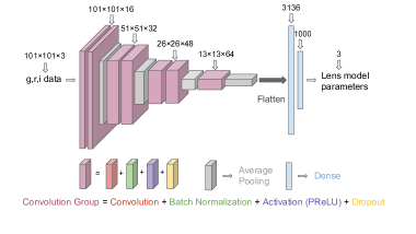
Figure 1: Network Architecture

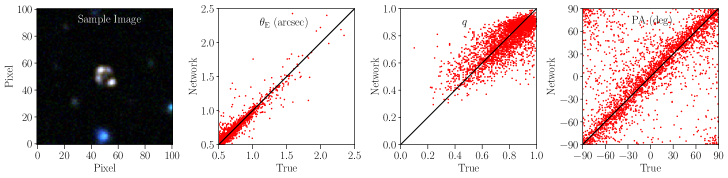
Figure 2: Performance of our network on a test sample of 2850 lenses where simulated lensed sources are added to random HSC cutouts. In this case both the training and test set images have similar features represented by the sample image in the first panel. The size of the training and test image cutouts in pixels is $101\times 101$ which corresponds to the angular size of $17$ arcsec $\times$ $17$ arcsec approximately. The second, third and fourth panels describe the predictions by our network for Einstein radius ($\theta_{\rm E}$), axis ratio ($q$) and position angle (PA) respectively as compared to the true values used to generate these simulated images.

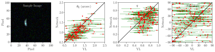
Figure 3: Performance of our network on a test set of 182 grade A and B SuGOHI lenses processed by YL. In this case the training set is the same as described in the Fig. 2. The test set consists of 182 grade A and B SuGOHI lenses processed using YL to remove the central lens light and foreground objects. The sample image in the first panel represents the test set as processed by YL. The second, third and fourth panels describe the predictions by our network for Einstein radius ($\theta_{\rm E}$), axis ratio ($q$) and position angle (PA) respectively as compared to the values predicted by YL along with their errors.

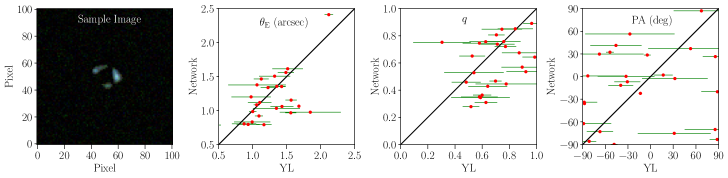
Figure 4: Performance of our network on a test set of 25 grade A SuGOHI lenses processed by YL which is actually a subset of the test set described in the Fig. 3. We can see that the scatter in the predictions of grade A SuGOHI lenses appear to be similar to that of predictions of the combined grade A and B SuGOHI lenses qualitatively and focusing on the grade A lenses does not lead to any significant improvement in the results.

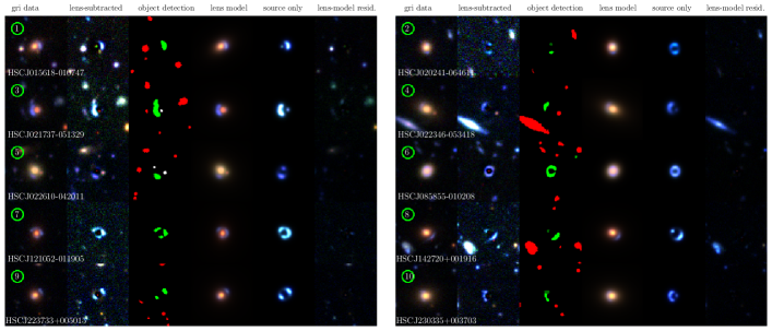
Figure 5: A sample of colour-composite images of 10 SuGOHI lenses commonly modelled in S19, S23, YL and our work. We have processed these lenses using YL in order to remove the central lens light and foreground objects. Columns from left to right : original image, lens-subtracted image, arc and image segmentation map (green = arcs, white = modelled foreground objects, red = masked out foreground objects), best-fitting lens model of the system (including modelled foreground objects), best model of the lensed background galaxy alone (source only model), residuals between the data and the best-fitting lens model.

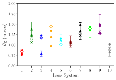
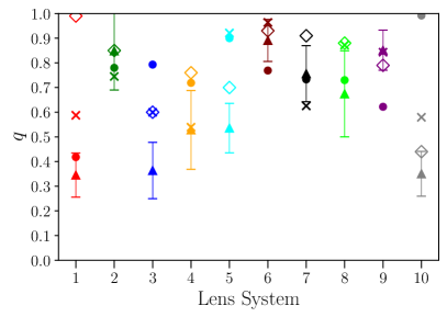
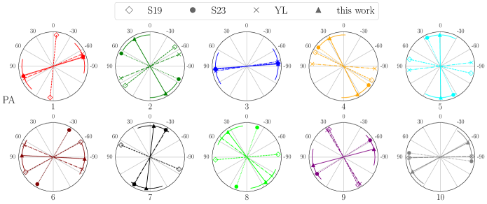
Figure 6: Comparison of the the lens model parameters, namely, Einstein radius ($\theta_{\rm E}$), axis ratio ($q$) and position angle (PA) predicted by our network (this work) with YL, S19 and S23 results. The error bars on our network predictions are obtained by quantifying the scatter in the network predictions on a simulated test sample shown in Fig. 2. We convert the results of YL, S19 and S23 for $\theta_{\rm E}$ and PA to our conventions before comparing (see Appendix A).

Table 1: Lens model parameters predicted by our network for 10 SuGOHI lenses that are also modelled in S19, S23 and our analysis with YL. The errors are obtained by quantifying the scatter in the network predictions on a simulated test sample shown in Fig. 2 and the error in PA is approximately $\pm 30$ degrees.

ID	Name	$\theta_{\rm E}$ (arcsec)	$q$	PA (deg)
1	HSCJ015618-010747	$0.80\pm 0.07$	$0.35\pm 0.09$	$-73$
2	HSCJ020241-064611	$1.38\pm 0.18$	$0.85\pm 0.16$	$30$
3	HSCJ021737-051329	$0.79\pm 0.06$	$0.36\pm 0.11$	$-86$
4	HSCJ022346-053418	$1.2\pm 0.15$	$0.53\pm 0.16$	$26$
5	HSCJ022610-042011	$1.12\pm 0.14$	$0.54\pm 0.10$	$1$
6	HSCJ085855-010208	$1.08\pm 0.14$	$0.89\pm 0.09$	$87$
7	HSCJ121052-011905	$1.34\pm 0.20$	$0.76\pm 0.11$	$-7$
8	HSCJ142720+001916	$1.36\pm 0.17$	$0.67\pm 0.17$	$37$
9	HSCJ223733+005015	$1.5\pm 0.23$	$0.85\pm 0.08$	$-75$
10	HSCJ230335+003703	$0.83\pm 0.11$	$0.35\pm 0.09$	$-62$

4 Results and Discussion

We train our network using simulated lenses and their SIE lens model parameters Einstein radius, axis ratio and position angle (see Appendix A for conventions) and apply it to simulated as well as real SuGOHI lenses to estimate the same parameters. Amongst the three parameters Einstein radius is the most crucial parameter to describe the lens mass distribution and it is also the most robust parameter to predict as it mostly depends on just the radial distances of the lensed arcs from the central lens galaxy. However, axis ratio and position angle are related to the actual configuration of the lensed arcs and are tricky to infer. We test the network on the simulated lenses as we have true model parameters for comparing the network predictions. In addition as mentioned previously, we also test on few of the SuGOHI lenses that have been already modelled in the literature. It was a challenge to find reliable parameters for these real lenses to compare the predictions from our network. To address this issue, we run a traditional MCMC modelling pipeline YL on the SuGOHI lenses to obtain the lens model parameters and compare our network predictions with the estimations from YL.

When we train any CNN on a training sample which contains images having specific features, the network learns those features during the training process and we expect it to perform well when tested on the images having similar features. As a result, the performance of our network on the real SuGOHI lenses hugely depends on how well our simulated training images resemble the real SuGOHI lenses. As discussed in Section 2.1, we tried different training samples with various degrees of realism and we briefly describe the results here. We split each sample of simulated lenses in a training and a test sample. After training our network on a particular simulated training sample, we test it on the simulated as well as the real SuGOHI test sample (lens light removed by YL).

The training sample a, where we convolve our simulated arcs with the PSF and add Poisson noise to them without adding any background noise is a very ideal case. When we train our network with this sample, it produces really good results on the simulated test sample but fails miserably on the real SuHOHI lenses due to missing features like background noise in the training data. In order to address this issue, we create the training sample b where we add Gaussian background noise to the training sample a. Training the network with the sample b improves the performance of the network on the real SuGOHI test images, however the results were still not satisfactory.

Therefore, we decide to produce sample c by adding the simulated arcs to the image cutouts of the respective HSC galaxy (central lens galaxy used to model the arcs). Although this sample resembles well with the real SuGOHI lenses (not processed by YL) having the real background noise along with the light from the central lens galaxy, when we train our network on this sample, it performs poorly on the real data when compared with the predictions from YL (see Appendix B). The reason for this failure is network’s inability to model the light coming from the central lens galaxy, which either outshines or contaminates the background lensed arcs in most of the cases. This necessitates modelling and subtracting the lens light before feeding the images to the network and we use YL pipeline for this purpose. The training sample d is produced by processing the sample c with YL, identically as we process the real SuGOHI lenses to subtract the lens light. When we train our network on the training sample d, surprisingly it fails on both the simulated as well as real lenses, especially in predicting the axis ratio and the position angle. We investigate this issue further by performing different sanity checks with YL. Our experiments show that processing the lenses via YL to remove light from the central lens often introduces uncertainties in the lensed configuration, particularly, for lenses with small Einstein radii, either by leaving a residue or over-subtracting the flux. Even though the Einstein radius is a robust parameter to infer, it seems that the axis ratio and the position angle are quite sensitive to these uncertainties.

Thus, we finally create a training sample with a technique that does not involve adding or subtracting the lens light but has real foregrounds and backgrounds. We add our simulated lensed arcs to selected cutouts from HSC with central empty regions as discussed while concluding the Section 2.1 and use this training sample to produce all of the results shown in this paper. We have also compared our results for a subset of the SuGOHI lenses with the analysis done in S19 and S23 as we describe in the following sections.

4.1 Performance on simulated and real lenses

The performance of our network on the simulated test sample is shown in Fig. 2. In this plot, we compare the lens model parameters estimated by our network with the true lens model parameters that we used to simulate these lenses. We can see from the sample image in Fig. 2 that these simulated lenses have noisy features similar to the real SuGOHI lenses as we have added the simulated arcs to real HSC cutouts as described in the subsection  2.1. Our network performs reasonably in predicting the lens model parameters for the simulated lenses. Our network is able to recover the Einstein radius really well, while the scatter in the axis ratio and position angle is also within acceptable limits considering the difficulty in estimating these two parameters. We have also tested our network on the real SuGOHI grade A+B lenses as shown in the Fig. 3 and on a subsample consisting of only grade A lenses as shown in the Fig. 4. In Fig. 3 and Fig. 4, we compare the lens model parameters estimated by our network with the parameters predicted by YL along with their uncertainties. We can see that the quality of results on both the A+B and grade A lenses is similar, suggesting no peculiar advantage in selecting just the grade A lenses. The predictions from our network and YL mostly agree within the acceptable limits for the Einstein radius, while there is a quite disagreement between the two for axis ratio and position angle.

The two main challenges we faced while testing our network on the real lenses is lens-light subtraction and obtaining the true parameters of real lenses to compare our network predictions with. Generally in a lens system, the central lens galaxy outshines the lensed galaxies in the background and blending can further make it difficult to identify the lensed arcs. So, this contamination caused by the central lens light prompts us to remove it before feeding the image to the network. While we have conveniently avoided adding the lens light in the simulated images, we don’t have this liberty for the real lenses and we had to find a method to remove it. Nevertheless, quite a few of these SuGOHI lenses have been rigorously modelled in the literature, making it difficult to obtain reliable benchmarks for a larger sample to compare our results with. To address both of these aforementioned issues, we decided to use YL pipeline with some minor changes suited for our analysis.

A sample of SuGOHI lenses processed by YL is shown in the Fig. 5. YL first models the light from the foreground lens galaxy in the centre and removes it to improve the identification of the lensed arcs in the background as shown in the second column (lens-subtracted) of Fig. 5. It then distinguishes potential lensed arcs from the foreground objects as shown in the segmentation map in the third column (object detection) of Fig. 5. YL then fits the SIE model to the lensed arcs in the lens light subtracted image as shown in the fourth column (lens model) of Fig. 5. YL also estimates the lens model parameters which we have used as benchmarks to compare our results with as shown in the Fig. 3 and Fig. 4. The errors on these parameters are from the 68 percent credible intervals from the posterior distribution of the parameters given the lens subtracted image, and obtained using a Monte Carlo Markov Chain.

We find that the predictions for Einstein radius by YL and our network are in good quantitative agreement, although the axis ratio and the position angle fair poorly. However, axis ratio and position angle are quite sensitive to the actual arc configuration. When we process the SuGOHI lenses using YL to remove the central lens light, sometimes the pipeline does not perform well either leaving a residue from the central lens light or modelling a part of the lensed source as a lens light and then subtracting it. As a result the lens light subtraction process leaves its imprints which contaminates the actual configuration of lensed arcs, further leading to erroneous predictions of the lens model parameters by YL. The huge uncertainties on the parameter estimation from YL shown by the green error bars is also a concern. Given these issues, one may question the reliability of the parameters obtained by YL. To address this we also judge the performance of our network on the real SuGOHI lenses obtained from other competing methods as described in the next subsection.

4.2 Comparison with S19 and S23

For this purpose, we select 10 grade A SuGOHI lenses (see Fig. 5 and Table 1) that were also modelled by S19 and S23. In S19, they modelled a sample of 23 strong lenses from the constant mas (CMASS) sample of Baryon Oscillation Spectroscopic Survey (BOSS) galaxies for which HSC imaging data in g, r, i, z and y bands is available. They model the lens mass with a SIE profile running a MCMC code, using the software EMCEE (Foreman-Mackey et al., 2013).

In S23, they applied a CNN to 31 grade A real galaxy-scale lenses from SuGOHI and compared their results with traditional, MCMC sampling-based models obtained from their pipelines GLEE & GLAD. They also compared the results obtained from GLEE and GLAD with the results presented in S19 for some lenses common in both the analysis as shown in the fig.3 of S23. While both of these methods agree well on the predictions of Einstein radius, they often differ significantly for the axis ratio and position angle (often beyond the quoted uncertainties). The fact that S19 uses SIE-only model, where GLEE and GLAD uses SIE+external shear model, alone is not enough to justify the discrepancy (see discussion in S23).

We process this sample of 10 grade A SuGOHI lenses using YL as shown in Fig. 5 in order to remove the central lens light and foreground objects in order to feed it to our network. We compare predictions from our network with the traditional MCMC modelling results presented in S19 and S23 in Fig. 6. We convert the Einstein radius and position angle from the other two methods to our convention before comparing (see Appendix A). The errors in Fig. 6 are obtained by quantifying the scatter in the network predictions on a simulated test sample shown in Fig. 2.

Here, we first describe our inferences from the visual comparison of the lens models shown in S19 (see fig. 1 in Sonnenfeld et al., 2019), S23 (see fig. B.1 - fig. B.31 in Schuldt et al., 2023) and YL (see Fig. 5). Next, we give a quantitative comparison of the model parameters from this work (Fig. 6) and the other studies. The errorbars mentioned in the following text and as shown in the (Fig. 6) are 1 $\sigma$ errorbars from our network predictions and are obtained by quantifying the scatter in the network predictions on a simulated test sample shown in Fig. 2.

1. HSCJ015618-010747 : In this case, the models of YL, S19 and S23 (see their fig. B.1) are visually similar. The axis ratio, $q$, predicted by S19 is close to unity and poses difficulty in constraining the PA which deviates from other results. The $q$ values predicted by S23 and network are within the quoted errorbars. The predictions for PA are within the errorbars for YL, S23 and network, while the predictions for $\theta_{\rm E}$ are close enough for all the methods.

2. HSCJ020241-064611 : For this lens, the models of YL, S19 and S23 (see their fig. B.3) look qualitatively similar with one image in the north and the other in the south direction. The model parameters $\theta_{\rm E}$ and $q$, for all four methods, are roughly consistent within the quoted errorbars due to the similarity of models containing two compact images, whereas the PAs of the mass distribution are harder to constrain due to their low ellipticities (i.e. high $q$).

3. HSCJ021737-051329 : The best-fit models of this lens by YL, S19 and S23 (see their fig. B.5) are similar and agree well on $\theta_{\rm E}$. Our $\theta_{\rm E}$ shows deviation from other methods. The PA is robustly constrained as all the methods give strongly consistent predictions. The predicted axis ratios are comparable for S19 and YL but the other two methods are not consistent with this, making $q$ the least well-constrained parameter despite the apparent similarity in their mass models.

4. HSCJ022346-053418 : Since the counter image of the arc, if any, is barely visible in this lens, we expect that the degeneracies in various models will become more apparent here. The model images of YL, S19 and S23 (see their fig. B.6) are visually similar. The model parameters $\theta_{\rm E}$ and $q$, for all four methods, are roughly consistent within the quoted errorbars. The PAs from S19, S23 and network are also approximately consistent within the errorbars, while the PA from YL deviates from this.

5. HSCJ022610-042011: In this case, the lens produces two images of the source galaxy. The model parameter $\theta_{\rm E}$, for all four methods, is consistent. There are differences in the predicted values of the axis ratio of the lensing potential, although all predictions are $>0.5$. We find that the axis ratio predicted by YL and S23 (for model, see their fig. B.7) agree well while those from S19 and network and are roughly within the errorbars. The PAs from S23 and network are within the quoted errorbars, while YL and S19 predict PA values which are close. The overall circularity ($q>0.5$) of the system implies that the position angle is hard to constrain and that can be seen from the large mismatch of the PAs inferred from the different methods as shown in Fig. 6.

6. HSCJ085855-010208 : The lens subtracted image in this lens system shows a near Einstein ring which is typical for a system with axial symmetry and a perfect alignment of the source with the lens center. The models from YL, S19 and S23 (see their fig. B.11) all reflect this feature resulting in values of the axis ratios close to unity for the lens model. The radius of the near perfect Einstein ring further helps each of the models to constrain the parameter $\theta_{\rm E}$ in a consistent manner. However, the inference of the PA is quite uncertain given the axial symmetry.

7. HSCJ121052-011905 : In this case, we can see the 3 images almost making an Einstein ring but two of them (the north-east and the west images) have extended structures deviating from the tangential direction. The models of YL and S19 are similar although the source of S19 is more compact than that of YL. These models lead to more smooth and circular configuration than the actual system. The S23 (see their fig. B.15) source model is more clumpy and does not have extended features. The inferred $\theta_{\rm E}$ agree with each other because of the similar angular separations of the arcs from the center of the lens potential. The model parameter $q$, predicted by all four methods is consistent within the errorbars. The PAs from YL, S23 and network are within the quoted errorbars, while the PA from S19 deviates from this.

8. HSCJ142720+001916 : For this lens, S19 and S23 (see their fig. B.22) models appear more accurate with an extended source whereas YL model is more circular with a compact source. The models from all methods agree well on $\theta_{\rm E}$ and the predictions for $q$ are also within the errorbar from our network. The inferred PA from S19 and S23 are distinct from both YL and our network, where the latter two are more consistent with each other.

9. HSCJ223733+005015 : In this case, YL and S19 models contain two diametrically opposite images and these models are qualitatively similar and accurate. As a result, these two methods also agree on the predictions of all the three parameters. The model of S23 (see their fig. B.27) does not seem correct with an arc modelled incorrectly in the south-east direction. However, the results of S23 for $\theta_{\rm E}$ and PA are within the errorbars from the network.

10. HSCJ230335+003703 : For this quad lens system, S19 model looks quite accurate with distinct four images of a compact source. The lens model of YL does not seem accurate. It has an extended source and the model looks more circular than the actual configuration of the lensed images. The model of S23 (see their fig. B.28) also does not do justice to the actual configuration.The inferred PAs from YL, S19 and S23 agree well and are within the errrorbars from the network. The $\theta_{\rm E}$ for all the methods is roughly consistent within the quoted errorbars. The axis ratio is not constrained well for this lens.

After comparing results from the three conventional modelling methods, namely, YL, S19 and S23 with our network, we realise that even though these methods are modelling the same SuGOHI lenses with identical data quality, other than the Einstein radius, a consensus in the predicted parameters is difficult to achieve. We note that this trend is seen, in spite, of other teams having modelled the 10 systems individually and using highly sophisticated methods. A similar inference is made in S23 as well. Such discrepancies could be due to the differences in the actual algorithms involved in modelling the lens systems. For instance, techniques used for modelling the light profile of the lens galaxy and the source, the choice of including or excluding the external shear and using different combinations of the broad-band data. In addition, the actual mass model of the galaxy can be quite complicated than the SIE+external shear model. However, in the absence of the ground truth, one cannot assess which of the methods and their results are more accurate. It may well be that the limitation is inherent to the quality and resolution of the ground-based survey data and better accuracy on the parameters is not possible unless working with data from space based surveys like the Hubble Space Telescope (e.g., Hezaveh et al., 2017).

5 Summary and Conclusion

In the era of next generation surveys with expected number of strong lenses to be $\mathcal{O}(10^{4})$, we will not have enough resources to model each lens at a time to determine the lens parameters. In this work, we aim to analyse the strong lenses from ground-based imaging surveys in a fast and automated way to prepare ourselves for the big data expected from surveys such as the Rubin LSST. Analysis of images of strong lens systems from a ground-based survey presents a challenge, as the imaging is limited by poor image quality due to atmospheric seeing and low angular resolution. Additionally, increasing depths of the surveys implies increased number of lenses at higher redshifts where the lensed images can often be faint.

To this end, we developed a simple CNN to analyse the strong lenses from the HSC data, a precursor to Rubin LSST, and estimate the lens model parameters. We first trained and tested our network on 60000 HSC-like galaxy-scale simulated lenses to predict the following three parameters of the SIE lens mass model, namely, the Einstein radius, the axis ratio and the position angle of the major axis of the mass distribution. Once we optimise our network on the simulated data, we then tested it on the real galaxy-scale lenses from SuGOHI to predict the aforementioned parameters. We compared our model predictions for 10 SuGOHI lenses that are also modelled by others in the literature with conventional MCMC modelling methods.

Our network performs reasonably well on the simulated lenses in recovering lens model parameters, especially, the Einstein radius which is the most crucial parameter in inferring the mass. For real lenses, we do not have the ground truth for parameters, like we have for the simulated lenses, to compare the predictions from our network in order to gauge its performance. Thus, after applying our network on the sample of 182 SuGOHI (candidate) lenses, we compare our results with the prediction from the YL pipeline. The predicted Einstein radii are generally consistent from the two methods within the errors given by YL. The predictions for the axis ratios and the position angles, however, are not as robust and the degree to which both methods agree varies across the lens sample.

For the 10 SuGOHI lenses which are common to S19, S23 and our analysis with YL and the network, we found similar results as before. The Einstein radius is a fairly robust parameter to infer but the axis ratio and position angle show large variations when inferred even with sophisticated and detailed MCMC modelling carried out on individual lenses (e.g. S19 and S23).

We also note that processing the SuGOHI lenses via YL to remove the central lens light may introduce uncertainties in the lensed images, particularly, for small Einstein radii system, either by leaving a residue or over-subtracting the flux. This can further contribute to the uncertainties in the parameter estimation. In the near future, we plan to work on developing a better method to simultaneously model the lens light along with the lens mass to minimise some of these uncertainties. We also plan to incorporate more of the lens and source parameters in our computation along with analysing how the performance varies as a function of SNR, number of detected images and presence of foreground contaminants. We also look forward to study and implement interpretability tools for CNNs to understand the modelling by our network and its failure modes. We aim to extend this work to upcoming ground based surveys like LSST.

Data Availability

The SuGOHI lenses and the YattaLens  pipeline used in this paper are publicly available. The CNN code and simulated images can be made available upon a reasonable request to the corresponding author.

Appendix A Our conventions for Einstein radius and Position Angle

We convert the Einstein radius values quoted in S19 and S23 to our convention (GRAVLENS, Keeton et al., 2000) using the following relation :

$$\theta_{\rm E}=\sqrt{\frac{2q}{1+q^{2}}}\theta_{\rm E}^{\rm S19}=\sqrt{\frac{2q}{1+q^{2}}}\theta_{\rm E}^{\rm YL}=\sqrt{\frac{2q}{1+q^{2}}}\frac{2\sqrt{q}}{(1+q)}\theta_{\rm E}^{\rm S23}$$ (2)

where, $q$ is the ratio of semi-minor to semi-major axis of the mass distribution of the SIE. We measure the position angle East of North as shown in the Fig. 6 and convert the position angle values quoted in S19 and S23 to this convention before comparing. These conversions were derived by equating the form of the convergence assumed in each of these methods.

Appendix B Analysis of lenses with the lens light

In the Section 2.1, we mentioned the training sample c, where we add simulated arcs (PSF-convolved and Poisson noise added) to the image cutout of the corresponding central HSC galaxy used to model the arcs. Analysing this training sample is important as it resembles the real SuGOHI lenses (not processed by YL), having the real background noise along with the light from the central lens galaxy. When we train our network on this training sample $c$ and test it on the corresponding simulated test sample (see Fig. 7), we find that Einstein radius is not well-constrained. The network recovers the axis ratio and position angle of the mass distribution fairly well because while simulating the lenses, the axis ratio and the position angle of the lens mass model is considered to be the same as that of the lens light. As a result, the presence of the lens light helps the network to estimate the axis ratio and position angle better.

When we test our network on the real lenses available in the SuGOHI database, which inherently contain the lens light, it performs poorly when compared to the predictions from YL (see Fig. 8 and Fig. 9). In the real lenses from the SuGOHI sample, the light coming from the central lens galaxy, either outshines or contaminates the background lensed arcs in most of the cases, which makes it difficult for the network to detect and study the lensed sources. Besides, for real lenses, the axis ratio and position angle of the lens mass model can be quite different from that of the lens light, making the presence of the lens light an issue. This analysis along with Hezaveh et al. (2017), prompted us to perform lens light subtraction and we have used YL for the same.

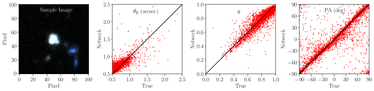
Figure 7: Performance of our network on a test sample of 2850 lenses where simulated lensed sources are added to the cutouts of central HSC galaxies used as lenses to simulate the lensed arcs. In this case both the training and test set images have similar features represented by the sample image in the first panel. The size of the training and test image cutouts in pixels is $101\times 101$ which corresponds to the angular size of $17$ arcsec $\times$ $17$ arcsec approximately. The second, third and fourth panels describe the predictions by our network for Einstein radius ($\theta_{\rm E}$), axis ratio ($q$) and position angle (PA) respectively as compared to the true values used to generate these simulated images.

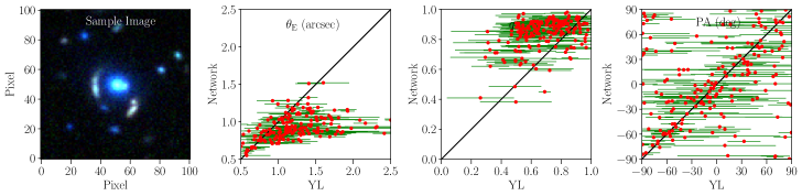
Figure 8: Performance of our network on a test set of 182 grade A and B SuGOHI lenses. In this case the training set is the same as described in the Fig. 7. The sample image in the first panel represents the test set consisting of grade A and B lenses available in the SuGOHI database without any further processing. The second, third and fourth panels describe the predictions by our network for Einstein radius ($\theta_{\rm E}$), axis ratio ($q$) and position angle (PA) respectively as compared to the values predicted by YL along with their errors.

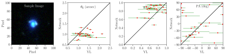
Figure 9: Performance of our network on a test set of 25 grade A SuGOHI lenses which is actually a subset of the test set described in the Fig. 8. We can see that the scatter in the predictions of grade A SuGOHI lenses appear to be similar to that of predictions of the combined grade A and B SuGOHI lenses qualitatively and focusing on the grade A lenses does not lead to any significant improvement in the results.

References

- Allingham et al. (2023) Allingham J. F. V., et al., 2023, MNRAS, 522, 1118
- Auger et al. (2010) Auger M. W., Treu T., Bolton A. S., Gavazzi R., Koopmans L. V. E., Marshall P. J., Moustakas L. A., Burles S., 2010, ApJ, 724, 511
- Foreman-Mackey et al. (2013) Foreman-Mackey D., Hogg D. W., Lang D., Goodman J., 2013, PASP, 125, 306
- Gentile et al. (2023) Gentile F., Tortora C., Covone G., Koopmans L. V. E., Li R., Leuzzi L., Napolitano N. R., 2023, MNRAS, 522, 5442
- Hezaveh et al. (2017) Hezaveh Y. D., Levasseur L. P., Marshall P. J., 2017, Nature, 548, 555
- Jacobs et al. (2017) Jacobs C., Glazebrook K., Collett T., More A., McCarthy C., 2017, Monthly Notices of the Royal Astronomical Society, 471, 167
- Jaelani et al. (2023) Jaelani A. T., More A., Wong K. C., Inoue K. T., Chao D. C. Y., Premadi P. W., Cañameras R., 2023, arXiv e-prints, p. arXiv:2312.07333
- Keeton et al. (2000) Keeton C. R., Christlein D., Zabludoff A. I., 2000, ApJ, 545, 129
- Koopmans et al. (2006) Koopmans L. V. E., Treu T., Bolton A. S., Burles S., Moustakas L. A., 2006, ApJ, 649, 599
- Levasseur et al. (2017) Levasseur L. P., Hezaveh Y. D., Wechsler R. H., 2017, The Astrophysical Journal Letters, 850, L7
- Limousin et al. (2009) Limousin M., et al., 2009, A&A, 502, 445
- More et al. (2012) More A., Cabanac R., More S., Alard C., Limousin M., Kneib J.-P., Gavazzi R., Motta V., 2012, The Astrophysical Journal, 749, 38
- More et al. (2016) More A., et al., 2016, MNRAS, 455, 1191
- Moriwaki et al. (2023) Moriwaki K., Nishimichi T., Yoshida N., 2023, Reports on Progress in Physics, 86, 076901
- Newman et al. (2013) Newman A. B., Treu T., Ellis R. S., Sand D. J., 2013, ApJ, 765, 25
- Nightingale et al. (2021) Nightingale J., et al., 2021, The Journal of Open Source Software, 6, 2825
- Nord et al. (2020) Nord B., et al., 2020, MNRAS, 494, 1308
- Oguri et al. (2012) Oguri M., Bayliss M. B., Dahle H., Sharon K., Gladders M. D., Natarajan P., Hennawi J. F., Koester B. P., 2012, MNRAS, 420, 3213
- Oguri et al. (2014) Oguri M., Rusu C. E., Falco E. E., 2014, Monthly Notices of the Royal Astronomical Society, 439, 2494
- Rojas et al. (2022) Rojas K., et al., 2022, A&A, 668, A73
- Schuldt et al. (2023) Schuldt S., Suyu S. H., Cañameras R., Shu Y., Taubenberger S., Ertl S., Halkola A., 2023, A&A, 673, A33
- Shajib et al. (2021) Shajib A. J., Treu T., Birrer S., Sonnenfeld A., 2021, MNRAS, 503, 2380
- Sonnenfeld et al. (2015) Sonnenfeld A., Treu T., Marshall P. J., Suyu S. H., Gavazzi R., Auger M. W., Nipoti C., 2015, ApJ, 800, 94
- Sonnenfeld et al. (2018) Sonnenfeld A., et al., 2018, PASJ, 70, S29
- Sonnenfeld et al. (2019) Sonnenfeld A., Jaelani A. T., Chan J., More A., Suyu S. H., Wong K. C., Oguri M., Lee C.-H., 2019, A&A, 630, A71