NEOMOD 3: The Debiased Size Distribution of Near Earth Objects

Abstract

Our previous model (NEOMOD2) for the orbital and absolute magnitude distribution of Near Earth Objects (NEOs) was calibrated on the Catalina Sky Survey observations between 2013 and 2022. Here we extend NEOMOD2 to include visible albedo information from the Wide-Field Infrared Survey Explorer. The debiased albedo distribution of NEOs can be approximated by the sum of two Rayleigh distributions with the scale parameters $p_{\rm V,dark}\simeq 0.03$ and $p_{\rm V,bright}\simeq 0.17$. We find evidence for smaller NEOs having (on average) higher albedos than larger NEOs; this is likely a consequence of the size-dependent sampling of different main belt sources. These inferences and the absolute magnitude distribution from NEOMOD2 are used to construct the debiased size distribution of NEOs. We estimate $830\pm 60$ NEOs with diameters $D>1$ km and $20,\!000\pm 2,\!000$ NEOs with $D>140$ m. The new model, NEOMOD3, is available via the NEOMOD Simulator – an easy-to-operate code that can be used to generate user-defined samples (orbits, sizes and albedos) from the model.

1 Introduction

An accurate knowledge of the size distribution of NEOs is interesting for many different reasons, including the objectives of the NASA’s Planetary Defense Coordination Office (PDCO). Several size-distribution models of NEOs have been developed (e.g., Mainzer et al. 2011, Morbidelli et al. 2020, Harris & Chodas 2021). Mainzer et al. (2011) combined the albedo measurements from the cryogenic portion of the Wide-Field Infrared Survey Explorer (WISE) mission with the magnitude distribution of known NEOs, approximately accounting for the incompleteness, to estimate $981\pm 19$ NEOs with $D>1$ km and $20,\!500\pm 3,\!000$ NEOs with $D>100$ m. The albedo distribution was inferred from NEOs detected by WISE, which was an appropriate choice because the WISE sample is much less biased with respect to visible albedo than surveys in visible wavelengths.

Morbidelli et al. (2020) developed an approximate debiasing method, combined the cryogenic WISE albedos with the NEO model from Granvik et al. (2018), and inferred $\sim 1000$ NEOs with $D>1$ km. The strength of this work relative to Mainzer et al. (2011) was that it used the debiased orbital and absolute-magnitude distribution model (Granvik et al. 2018; also see Bottke et al. 2002) – this removed uncertainties related to the completeness of the known NEO population considered in Mainzer et al. (2011). Morbidelli et al. (2020), however, used a relatively crude albedo binning (three bins with $p_{\rm V}<0.1$, $0.1<p_{\rm V}<0.3$ and $p_{\rm V}>0.3$; a uniform distribution assumed in each bin), which did not allow them to reconstruct the debiased albedo distribution in detail. The inferences given in that work for the size distribution of NEOs were therefore somewhat uncertain.

Finally, Harris & Chodas (2021) updated their previous model for the absolute magnitude distribution of NEOs (Harris & D’Abramo 2015). A reference albedo $p_{\rm V,ref}=0.14$ (Stuart & Binzel 2004) was used to convert the absolute magnitude distribution into the size distribution. This is less than ideal because NEOs have a wide range of visible albedos and it is therefore not obvious if there is a single albedo value that can be used to convert the distributions, and if so, what reference albedo should be used (Morbidelli et al. 2020 proposed $p_{\rm V,ref}=0.147$).

Here we combine the absolute magnitude distribution from NEOMOD2 (Nesvorný et al. 2024; hereafter Paper II) with the visible albedo information from WISE (Mainzer et al. 2011) to obtain the size distribution of NEOs.

NEOMOD is an orbital and absolute magnitude model of NEOs (Nesvorný et al. 2023; hereafter Paper I). To develop NEOMOD, we closely followed the methodology from previous studies (Bottke et al. 2002, Granvik et al. 2018), and improved it when possible. Massive numerical integrations were performed for asteroid orbits escaping from eleven main belt sources. Comets were included as the twelfth source. The integrations were used to compute the probability density functions (PDFs) that define the orbital distribution of NEOs (perihelion distance $q<1.3$ au, $a<4.2$ au) from each source. We developed a new method to accurately calculate biases of NEO surveys and applied it to the Catalina Sky Survey (CSS; Christensen et al. 2012) in an extended magnitude range ($15<H<28$). The MultiNest code (Feroz & Hobson 2008, Feroz et al. 2009) was used to optimize the (biased) model fit to CSS detections. The improvements included: (i) cubic splines to represent the magnitude distribution of NEOs, (ii) a physical model for disruption of NEOs at low perihelion distances (Granvik et al. 2016), (iii) an accurate estimate of the impact fluxes on the terrestrial planets, and (iv) a flexible setup that can be readily adapted to any current or future NEO survey. In Paper II (Nesvorný et al. 2024) we extended NEOMOD to incorporate new data from CSS.

Here we upgrade NEOMOD2 to include the WISE data. The main goal is to obtain an accurate estimate of the size distribution of NEOs. A straightforward approach to this problem would be to use the WISE measurements of NEO diameters, develop a debiasing procedure, and infer the size distribution from the WISE data alone. During the cryogenic portion of the mission, however, WISE only detected 428 unique NEOs (Mainzer et al. 2011), which can be compared to over $\sim 15,\!000$ unique NEO detections by CSS between 2013 and 2022. The results of the direct approach to this problem, as described above, would therefore suffer from (relatively) small number statistics. For this reason, it is better to use the WISE measurements of visible albedo of NEOs, debias them, and combine the results with the absolute magnitude distribution from NEOMOD2. This hybrid method takes advantage of the full statistics from CSS and the realistic albedo distribution from WISE.

We test several models with different parameters. The simple model and its variant with the size-dependent albedo distribution, as described in section 4.1, have fewer parameters and are therefore presumably more robust. We use these models to obtain population estimates and impact fluxes. The simple model cannot account for potential dependences of the albedo distribution on NEO orbit (e.g., outer main-belt sources may be producing more dark NEOs than the inner main-belt sources). We therefore develop a complex model where different NEO sources have different contribution to NEOs with low and high albedos (Sect. 4.2; Morbidelli et al. 2020). The complex model correctly reproduces the correlation of albedo with orbit inferred from the NEOWISE data, but it has more parameters, and at least in some cases MultiNest struggles to constrain them (e.g., the case of Phocaeas; Sect 4.2). The NEOWISE statistics with only 428 detections during the cryogenic part of the mission (Mainzer et al. 2011) may be not large enough for the complex model to fully converge to a perfect solution. In this situation, we find it best to stay conservative and report a relatively large range of estimates that contains the results of all explored models. Estimates for NEOs with diameters $D<100$ m are subject to additional uncertainties, as the albedo distribution for $D<100$ m needs to be extrapolated from the NEOWISE data for $D>100$ m.

2 The base model from Paper II

In NEOMOD2, the biased NEO model is defined as

$${\cal M}_{\rm b}(a,e,i,H)=n(H)\,{\cal P}(a,e,i,H)\sum_{j=1}^{n_{\rm s}}\alpha_{j}(H)\,p_{q^{*},j}(a,e,i,H)\,\ ,$$ (1)

where $n(H)$ is the differential absolute-magnitude distribution of the NEO population, ${\cal P}(a,e,i,H)$ is the CSS’s detection probability, $\alpha_{j}$ are the magnitude-dependent weights of different sources ($\sum_{j}\alpha_{j}(H)=1$), $n_{\rm s}$ is the number of NEO sources, $p_{q^{*},j}(a,e,i,H)$ is the PDF of the orbital distribution of NEOs from the source $j$, including the size-dependent disruption at the perihelion distance $q$ (Paper I).

The model domain in $a,e,i,H$ is divided into bins (see Table 2 in Paper I). To determine the survey’s detection probability in each bin, we place a large number of test bodies in each bin, assume random orbital longitudes, and test whether individual bodies are or are not detected. This includes considerations related to the geometric bias (i.e., will an object appear in survey’s fields of view?), photometric sensitivity and trailing loss (Paper II). ${\cal P}(a,e,i,H)$ is then calculated as the mean probability that an object with $a,e,i,H$ will be detected over the whole duration of the survey. The orbital distributions $p_{q^{*},j}(a,e,i,H)$ are obtained from numerical integrations described in Paper I. The distributions are normalized such that $\int p_{q^{*},j}(a,e,i,H)\ {\rm d}a\,{\rm d}e\,{\rm d}i=1$ for any $H$.

There are three sets of model parameters in NEOMOD2: the (1) coefficients $\alpha_{j}$, (2) parameters related to the absolute magnitude distribution of NEOs, and (3) priors that define the disruption model (Granvik et al. 2016). As for (1), we have $n_{s}=12$ sources in total: eight individual resonances ($\nu_{6}$, 3:1, 5:2, 7:3, 8:3, 9:4, 11:5 and 2:1), weak resonances in the inner belt, two high-inclination sources (Hungarias and Phocaeas), and comets. The intrinsic orbital distribution of model NEOs is obtained by combining all sources. The coefficients $\alpha_{j}$ represent the relative contribution of each source to the NEO population ($\sum_{j=1}^{n_{\rm s}}\alpha_{j}=1$). As the contribution of different sources to NEOs is size dependent (Papers I and II), $\alpha_{j}$ are functions of absolute magnitude; we adopt a linear dependence for simplicity. As for (2), the differential and cumulative absolute magnitude distributions are denoted $n(H)={\rm d}N/{\rm d}H$ and $N(H)$, respectively. We use cubic splines to represent $\log_{10}N(H)$ (Paper I). As for (3), we eliminate test bodies when they reach the critical distance $q^{*}(H)$. We assume that the $q^{*}$ dependence on $H$ is (roughly) linear, and parameterize it by $q^{*}=q_{0}^{*}+\delta q^{*}(H-H_{q})$, where $H_{q}=20$ (the choice of $H_{q}$ is arbitrary; $q_{0}^{*}$ and $\delta q^{*}$ are the model parameters).

The MultiNest code is used to perform the model selection, parameter estimation and error analysis (Feroz & Hobson 2008, Feroz et al. 2009). For each MultiNest trial, Eq. (1) is constructed by the methods described above. This defines the expected number of events $\lambda_{j}={\cal M}_{\rm b}(a,e,i,H)$ in every bin of the model domain, and allows MultiNest to evaluate the log-likelihood

$${\cal L}=-\sum_{j}\lambda_{j}+\sum_{j}n_{j}\ln\lambda_{j}\ ,$$ (2)

where $n_{j}$ is the number of objects detected by CSS in the bin $j$, $\lambda_{j}$ is the number of objects in the bin $j$ expected from the biased model, and the sum is executed over all bins in $a$, $e$, $i$ and $H$ (Paper I). There are 30 model parameters in total: 22 coefficients $\alpha_{j}$, 6 parameters that define the magnitude distribution from splines (five slopes and the overall normalization), and 2 parameters for the size-dependent disruption ($q_{0}^{*}$ and $\delta q^{*}$).

Once MultiNest converges, the maximum likelihood parameters can be used to define the intrinsic (debiased) NEO model

$${\cal M}(a,e,i,H)=n(H)\,\sum_{j=1}^{n_{s}}\alpha_{j}(H)\,p_{q^{*},j}(a,e,i,H)\,\ .$$ (3)

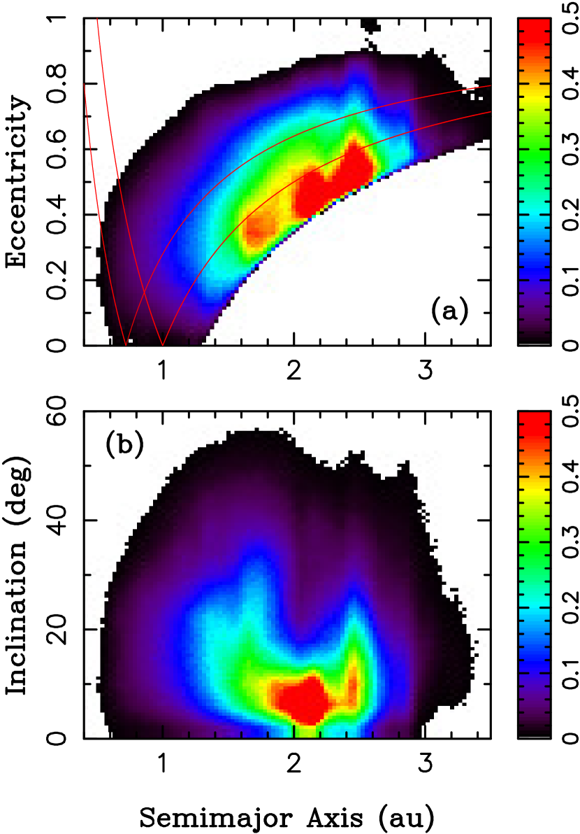
Figure 1: The orbital distribution of NEOs from our intrinsic (debiased) model (NEOMOD2). We used the NEOMOD Simulator (Paper II) and generated $1.1\times 10^{6}$ NEOs with $15<H<28$. The distribution was marginalized over absolute magnitude and binned using 100 bins in each orbital element ($0.4<a<3.5$ au, $e<1$ and $i<60^{\circ}$). Warmer colors correspond to orbits where NEOs are more likely to reside. In the plot shown here, the maximum residence probability in a bin is normalized to 1.

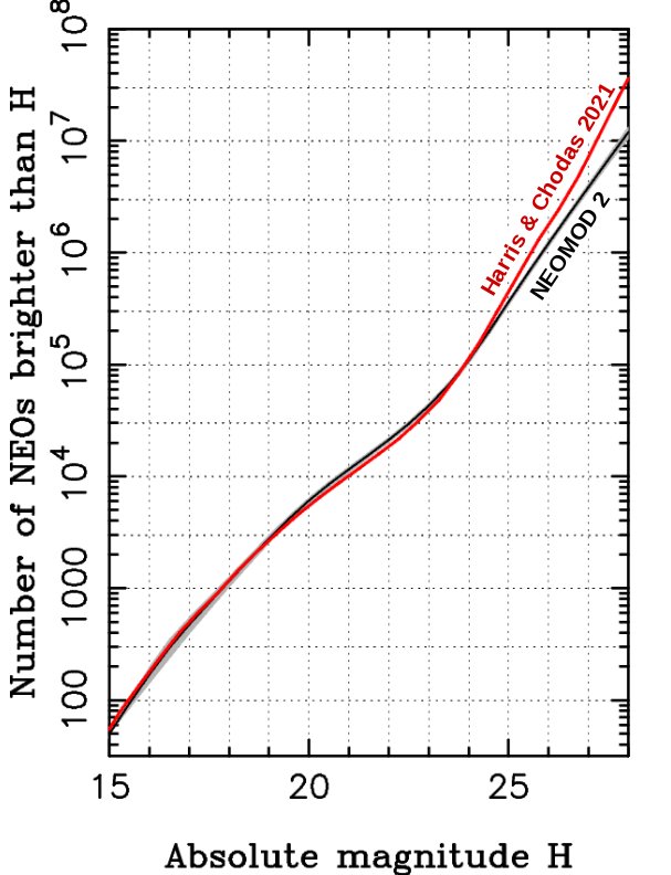
Figure 2: The intrinsic (debiased) absolute magnitude distribution of NEOs from NEOMOD2 (Paper II, the black line is a median) is compared to the magnitude distribution from Harris & Chodas (2021) (red line). The gray area is the 3$\sigma$ envelope obtained from the posterior distribution computed by MultiNest. It contains – by definition – 99.7% of our base model posteriors.

Figures 1 and 2 show the orbital and absolute magnitude distributions from NEOMOD2. The orbital distribution in Fig. 1 is consistent with the NEO model from Granvik et al. (2018). The absolute magnitude distribution in Fig. 2 is similar to the one reported in Harris & Chodas (2021, 2023) for $H<25$, but shows a shallower slope and fewer NEOs for $H>25$ (see Paper II for a discussion). It has to be noted that the distribution presented in Harris & Chodas (2021, 2023) assumed fixed slopes for $H>26$. This is because there is a statistially insignificant number of re-detection for $H>26$ and the re-detection method does not give useful results for these faint magnitudes.

3 Methods

3.1 NEO detections by cryogenic NEOWISE

WISE is a NASA mission designed to survey the entire sky in four infrared wavelengths: 3.4, 4.6, 12 and 22 $\mu$m, denoted $W1$, $W2$, $W3$ and $W4$, respectively (Mainzer et al. 2005, Liu et al. 2008). The survey began on January 14, 2010. The mission exhausted its primary tank cryogen on August 5, 2010 and secondary tank cryogen on October 1, 2010. An augmentation to the WISE processing pipeline, NEOWISE, permitted a search and characterization of moving objects. The survey has yielded observations of over 157,000 minor planets, including NEOs, main belt asteroids, comets, Trojans, Centaurs and Kuiper belt objects (Mainzer et al. 2011). The survey was continued as the NEOWISE Post-Cryogenic Mission using only bands $W1$ and $W2$.

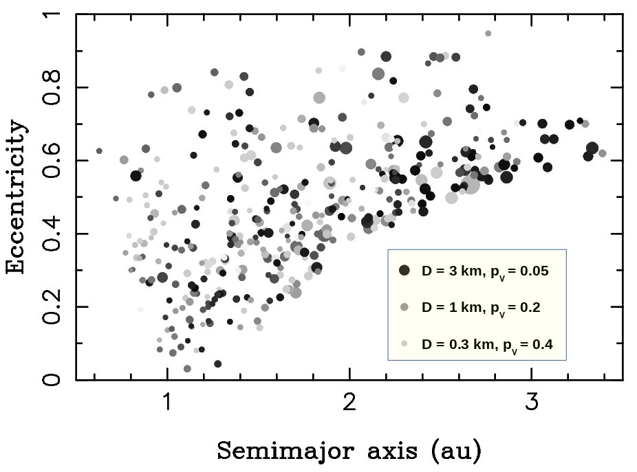
Figure 3: The orbits and albedos of 428 NEOs detected during the cryogenic portion of the WISE mission. The darker the dot, the lower the albedo. The size of a dot is proportional to asteroid diameter. There is a general trend with brighter asteroids being more prevalent for $a<2$ au (77% of NEOWISE NEOs have $p_{V}>0.1$) than for $a>2$ au (66% have $p_{V}>0.1$).

For the purposes of determining the debiased population of NEOs, in this paper, we only consider NEOs detected during the fully cryogenic portion of WISE. This data set consists of 428 NEOs (Fig. 3), of which 314 were rediscoveries of objects known previously and 114 were NEOWISE discoveries (Mainzer et al. 2011). The ranges of visual albedos, diameters and absolute magnitudes of NEOs detected by NEOWISE are $0.01<p_{\rm V}\lesssim 0.5$, $0.1<D<10$ km and $13\lesssim H\lesssim 23$, respectively.

The non-cryogenic portion of WISE is not considered here, because the $W1$ and $W2$ bands mix the reflected light with thermal emission, and are less useful for accurate albedo determinations. The cryogenic NEOWISE sample is only weakly biased with respect to visible albedo. For comparison, a survey in visible wavelengths such as CSS typically detects objects to some limiting apparent magnitude $V_{\rm lim}$. This results in a magnitude-limited sample where the population is characterized to some faint absolute magnitude limit, $H_{\rm lim}$; bodies with low visual albedos can be severely underrepresented for $H<H_{\rm lim}$ (Appendix A).

3.2 Thermal infrared bias

The intrinsic albedo distribution of NEOs is close but not exactly equal to that of NEOs detected by NEOWISE. This is because objects with low visible albedo absorb more sunlight and emit more thermal radiation; they are therefore more easily detected in infrared wavelengths. The NEOWISE sample is thus (slightly) biased toward NEOs with low visual albedos. This is only a modest effect for $D>1$ km (Mainzer et al. 2011), because large bodies with low and high albedos were detected nearly equally well by NEOWISE, but it can become increasingly important for $D<1$ km NEOs for which the thermal emission in the $W3$ band can be weak.

We used the Near-Earth Asteroid Thermal Model (NEATM) model (Harris 1998) to account for the thermal infrared bias. NEATM adopts several simplifying assumptions. Objects are assumed to be perfectly spherical. NEATM does not physically account for thermal inertia – it empirically models it using the beaming parameter, $\eta$. Mainzer et al. (2011) fitted $\eta$ for 313 NEOs with measurements in two or more thermal bands and found the median value $\eta=1.4$. We tested different values of $\eta$ in a 0.4 range around $\eta=1.4$ and found that the results are not sensitive to this choice. We therefore adopted $\eta=1.4$ as a fiducial value. The color corrections from Wright et al. (2010) were applied.

Here we model NEOWISE detections in the $W3$ band, which was available only during the cryogenic portion of the WISE mission, and had better sensitivity than the $W4$ band (surface temperatures of NEOs imply peak black body emission near the center of $W3$). The detection in the $W3$ band is therefore a good proxy for NEO detection by NEOWISE and a reliable measurement of asteroid albedo. The photometric detection probability of NEOWISE as a function of $W3$ magnitude was obtained as a ratio of detected and available NEOs in Mainzer et al. (2011). Adopting their Eq. (3), we have

$$P(W3)={\epsilon_{0}\over 1+\exp\left({W3-W3_{\rm lim}\over W3_{\rm wid}}\right)}$$ (4)

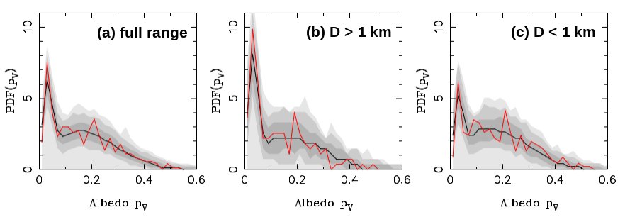
Figure 11: The (biased) albedo distribution from the complex model is compared to NEOWISE detections. From left to right the panels show the results for: (a) the full diameter range, (b) $D>1$ km, and (c) $D<1$ km. For $D>1$ km, the dark peak of the albedo distribution is prominent. For $D<1$ km, the dark peak is subdued, indicating that small NEOs more often have higher albedos. The model correctly reproduces the dependence of the albedo distribution on size.

with $\epsilon_{0}=0.9$, $W3_{\rm lim}=10.25$ and $W3_{\rm wid}=0.2$. This is the same functional form that we used to model CSS detections in the apparent magnitude $V$ in Paper I. The parameters $\epsilon_{0}$, $W3_{\rm lim}$ and $W3_{\rm wid}$ were fixed to provide the best fit to the median detection probabilities shown in Fig. 11 in Mainzer et al. (2011). We verified that small changes of these parameters do not substantially affect the results reported here.

To understand the thermal infrared bias in detail, we used the NEOMOD simulator (Paper II) and generated orbital elements $a$, $e$ and $i$ of $10^{5}$ model NEOs. The orbits were given a uniformly random distribution of orbital longitudes. For each diameter set, all bodies were assigned the same value of visible albedo $p_{\rm V}$ and the detection probabilities in the $W3$ band were computed individually for them. To respect the observing strategy of WISE, observations were assumed to happen in a narrow range of solar elongation about 90^∘. We then computed the average detection probability ${\cal P}(D,p_{\rm V})$ and analyzed it as a function of $p_{\rm V}$. This test shows that the detection probability is relatively insensitive to asteroid albedo, at least in the size range of NEOs detected by NEOWISE ($D\gtrsim 100$ m). For example, for $D=0.3$ km, the detection probability decreases from $\simeq 4.2$% for $p_{\rm V}=0$ to $\simeq 3.1$% for $p_{\rm V}=0.5$.

3.3 Albedo distribution

There are three model parameters related to the albedo distribution. Following Wright et al. (2016), we assume that the differential albedo distribution of NEOs can be approximated by a sum of two Rayleigh distributions

$$p(p_{\rm V})=f_{\rm d}{p_{\rm V}\over d^{2}}\exp\left(-{p_{\rm V}^{2}\over 2d^{2}}\right)+(1-f_{\rm d}){p_{\rm V}\over b^{2}}\exp\left(-{p_{\rm V}^{2}\over 2b^{2}}\right)\ ,$$ (5)

with parameters $f_{\rm d}$, $d$ (the scale parameter for low-albedo or $d$ark NEOs) and $b$ (the scale parameter for high-albedo or $b$right NEOs), where $f_{\rm d}$ is the fraction of NEOs in the low-albedo Rayleigh distribution (the first term in Eq. (5)). This functional form has fewer parameters than the double Gaussian distribution in Mainzer et al. (2011) and $p(p_{\rm V})$ falls to zero for $p_{\rm V}\rightarrow 0$ – a desirable property of any physical model.

Wright et al. (2016) determined $f_{\rm d}=0.253$, $d=0.030$ and $b=0.168$ for NEOs detected by cryogenic NEOWISE. Here we assume that Eq. (5) can be used for the debiased population as well and determine $f_{\rm d}$, $d$ and $b$ via the MultiNest fit. Mainzer et al. (2011) did not find any strong evidence for a correlation between albedo and size. For simplicity, we can thus assume that $f_{\rm d}$, $d$ and $b$ are unchanging with size (Sect 3.5).

3.4 Combining CSS and NEOWISE

The main objective of our work is to calibrate NEOMOD3 simultaneously from the CSS and NEOWISE data. CSS has a large number of detections, over $15,\!000$ NEOs from 2013 to 2022, which helps to accurately characterize the absolute magnitude distribution of NEOs as faint as $H=28$. The NEOWISE data set gives us the albedo distribution of NEOs and allows us to convert the absolute magnitude distribution into the size distribution (Sect. 3.8).

In Paper I, we described a method that can be used to combine constraints from any number of surveys, and illustrated it for the 703 and G96 telescopes. In Paper II, we used the same method to combine the G96 data from 2013–2016 (before the G96 camera upgrade) with the G96 data from 2016–2022 (after the G96 camera upgrade). The method consists in dealing with the surveys separately and evaluating the likelihood term in Eq. (2) for each of them. The likelihood terms of different surveys are then simply summed up. We previously developed and used this method for visible surveys but it can be used for infrared surveys as well.

To use this method here, we would need to compute the detection probability of NEOWISE as a function of the orbital elements $a,e,i$ (orbital longitudes can be ignored in the first approximation, but see JeongAhn & Malhotra 2014), absolute magnitude $H$ (or diameter $D$) and visible albedo $p_{\rm V}$. The detection probability has two parts: the geometric detection probability that an object will appear in WISE images and the photometric detection probability. The photometric detection probability is obtained from Eq. (4). To evaluate the geometric probability, we would need to collect the pointing history of WISE and link it with the Asteroid Survey Simulator (AstSim) package (Naidu et al. 2017), in much the same way this was done for CSS (Papers I and II). There would be no convenient way around this if the WISE observations were used on their own. Here, however, CSS provides a much stronger constraint on the absolute magnitude distribution. In this situation, it makes better sense to fix parameters of the base model from CSS (Paper II) and infer the (debiased) albedo distribution from NEOWISE.

3.5 Simple MultiNest fits

A simple (biased) visible-albedo model of the NEO population can be defined as

$${\cal M}_{\rm b}(p_{\rm V};a,e,i,D)={\cal P}(p_{V};a,e,i,D)\,p(p_{\rm V})\ ,$$ (6)

where ${\cal P}$ is the NEOWISE (photometric) detection probability (Sect. 3.2), and $p(p_{\rm V})$, as given in Eq. (5), is assumed to be independent of $a,e,i,D$. We consider 50 albedo bins for $0<p_{\rm V}<1$ and produce a binned version of ${\cal M}_{\rm b}$ (with the standard binning in $a,e,i$; Paper I). We only consider bins in $a,e,i,D$ where there were NEOWISE detections – all other bins are ignored. For each detected object, we find the bin in $(a,e,i,D)$ to which it belongs, and compute the detection probability ${\cal P}$ for fixed $a,e,i,D$ and changing $p_{\rm V}$. This is done by placing a large number of bodies in each albedo bin, adopting the same diameter for all of them from NEOWISE, running the NEATM model for all of them to determine the $W3$ magnitude in each case, and averaging the detection probability in the $W3$ band (Eq. 4) over the whole sample (Sect. 3.2).

In a bin $k$ in $(a,e,i,D)$, where there were $n_{k}=\sum_{l}n_{k,l}>0$ NEOWISE detections (typically $n_{k}=1$), where index $l$ runs over the albedo bins, we define $\lambda_{k,l}={\cal M}_{\rm b}(p_{\rm V};a,e,i,D)$ and normalize it such that $\sum_{l}\lambda_{k,l}=n_{k}$ (we are not interested in the absolute calibration). The log-likelihood in MultiNest is defined as

$${\cal L}=-\sum_{k,l}\lambda_{k,l}+\sum_{k,l}n_{k,l}\ln\lambda_{k,l}\ ,$$ (7)

where index $k$ runs over bins in $a,e,i,D$ with NEOWISE detections (and index $l$ over all albedo bins). MultiNest is then asked to determine parameters $f_{\rm d}$, $d$ and $b$ (Eq. 5) by maximizing the log-likelihood in Eq. (7). This gives us, via Eq. (5), the intrinsic (debiased) albedo distribution of NEOs. Note that the simple albedo model, as described here, does not need any input from NEOMOD.

3.6 Complex MultiNest fits

The simple albedo model can be generalized to account for the fact that different NEO sources may have different contribution to NEOs with low and high albedos (Morbidelli et al. 2020). This is done by generalizing $f_{\rm d}$ to have $n_{\rm s}=12$ coefficients $f_{{\rm d},j}$ that define the contribution of dark NEOs (i.e., NEOs in the low-albedo Rayleigh distribution in Eq. (5)) individually for each source. In this case, the biased model is defined as

$${\cal M}_{\rm b}(p_{\rm V};a,e,i,D)={\cal P}(p_{\rm V};a,e,i,D)\sum_{j=1}^{n_{s}}p_{j}(p_{\rm V})\,\alpha_{j}(H(D,p_{\rm V}))\,p_{q^{*},j}(a,e,i,H(D,p_{\rm V}))\,$$ (8)

with

$$p_{j}(p_{\rm V})=f_{{\rm d},j}{p_{\rm V}\over d^{2}}\exp\left(-{p_{\rm V}^{2}\over 2d^{2}}\right)+(1-f_{{\rm d},j}){p_{\rm V}\over b^{2}}\exp\left(-{p_{\rm V}^{2}\over 2b^{2}}\right)\ ,$$ (9)

being the albedo distribution of source $j$. Here, $H(D,p_{\rm V})=-5\log_{10}(D\sqrt{p_{\rm V}}/c)$ with $c=1329$ km (Russel 1916). The contributions of different sources, $\alpha_{j}(H)$, and $p_{q^{*},j}(a,e,i,H)$ are obtained from NEOMOD2 (these parameters are held fixed in the new fit). Again, as we are not interested in the absolute calibration, we define $\lambda_{k,l}={\cal M}_{\rm b}(p_{\rm V};a,e,i,D)$ and normalize it such that $\sum_{l}\lambda_{k,l}=n_{k}$. The MultiNest code is asked to determine the 14 parameters $f_{{\rm d},j}$, $d$ and $b$ by maximizing the log-likelihood in Eq. (7).

3.7 A note on coupling of model parameters

The two algorithms described in Sect. 3.5 and 3.6 represent a good compromise between: (1) simplicity (i.e., number of model parameters; complicated albedo models cannot be robustly constrained from the NEOWISE data), (2) realism (e.g., we cannot ignore obvious biases; Sects. 3.2 and 5.1), and (3) CPU expense. We experimented with several different methods. For example, we explored algorithms to simultaneously determine the CSS and NEOWISE parameters in a single fit. For the complex MultiNest fit (Sect. 3.6), this represents 30 model parameters for CSS and 14 parameters for NEOWISE (twelve coefficients $f_{{\rm d},i}$, $d$ and $b$). In this case, we obtained the same values (and uncertainties) of model parameters as in the method described in Sect. 3.6. This shows that the CSS and NEOWISE parameters are uncorrelated. The 44 parameter approach is, however, very CPU expensive.

3.8 From $H$ and $p_{\rm V}$ to the size distribution

It is not obvious how to convert the absolute magnitude and albedo distributions to the size distribution. This is because the albedo distribution, as obtained from NEOWISE,

$$\phi(p_{\rm V})={{\rm d}N\over{\rm d}p_{\rm V}}\Bigr{|}_{D={\rm const}}\ ,$$ (10)

is the albedo distribution of NEOs for a fixed size (or in a size range), and, for a simple conversion, we would need the albedo distribution for a fixed absolute magnitude (or in an absolute-magnitude range),

$$\phi^{\prime}(p_{\rm V})={{\rm d}N\over{\rm d}p_{\rm V}}\Bigr{|}_{H={\rm const}}\ .$$ (11)

These two albedo distributions are different, $\phi(p_{\rm V})\neq\phi^{\prime}(p_{\rm V})$, because the distribution in the absolute-magnitude range has a larger contribution of asteroids with higher albedos (Appendix A).

It can be shown that the three differential distributions, $n(H)={\rm d}N/{\rm d}H$, $\psi(D)={\rm d}N/{\rm d}D$ and $\phi(p_{\rm V})$ are related via the integral equation

$$n(H)={1\over\kappa}\int_{0}^{1}{\rm d}p_{\rm V}\,\phi(p_{\rm V})\,D\psi(D)\ ,$$ (12)

where $\kappa=-5/\ln 10$ and $D=D(H,p_{\rm V})=c10^{-H/5}/\sqrt{p_{\rm V}}$ ($D$ must be substituted for $H$ and $p_{\rm V}$ before the integral is evaluated). Eq. (12) needs to be solved to obtain $\psi(D)$. We experimented with several approaches to this problem. It turns out that Eq. (12) can be transformed, via substitutions of variables, to the integral Volterra equation of the first kind. It can be inverted to obtain $\psi(D)$ via the matrix inversion algorithm (Press et al. 1992) or Fourier transform (Muinonen et al. 1995).

We opted for a different method in this work. We assumed that $\psi(D)$ can be parameterized by cubic splines in much the same way as $n(H)$ (Paper I), used the same number of segments for $\psi(D)$ as for $n(H)$ and converted the segment boundaries from $H$ to $D$ with a reference albedo $p_{\rm V,conv}$. The Simplex algorithm from Numerical Recipes (Press et al. 1992) was then employed to minimize a $\chi^{2}$-like quantity, and find the (cumulative) power-slope indices $\beta_{j}$ in all segments, and $p_{\rm V,conv}$. This procedure works perfectly well (Section 4). We tested it by first determining $\psi(D)$, and then computing new $n(H)$ from $\psi(D)$ and $\phi(p_{\rm V})$ via Eq. (12); this recovers the original distribution $n(H)$ without any significant errors. The spline approach described here has the advantage of having $\psi(D)$ immediately represented by splines – the slopes in each segment have physical meaning and the size distribution is easy to generate (e.g., in NEOMOD Simulator).

4 Results

4.1 Simple fits

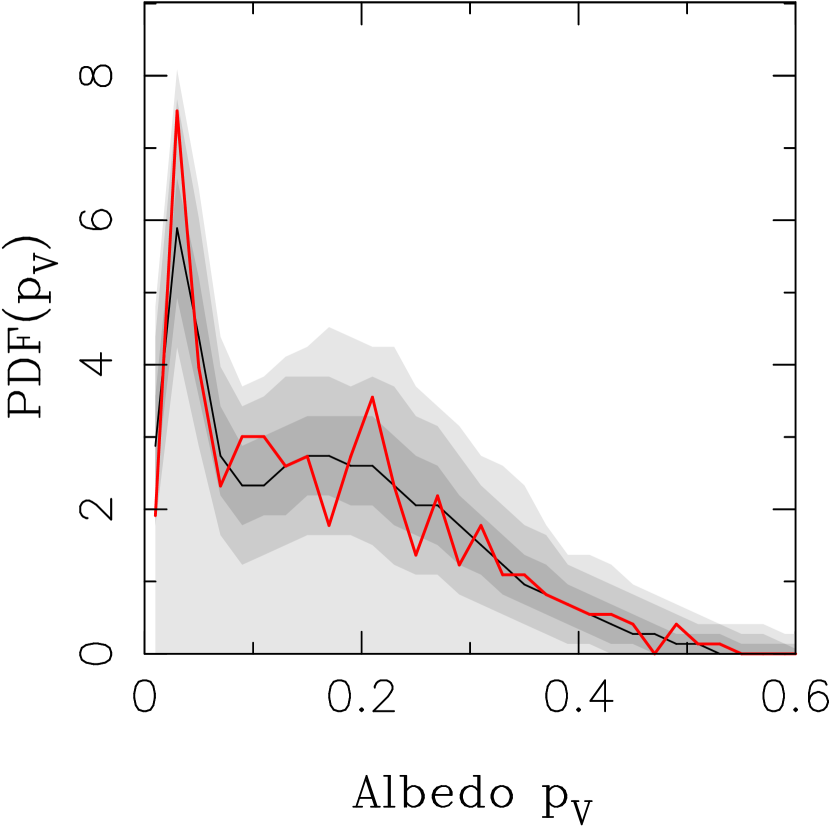
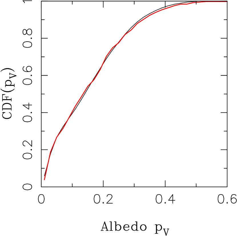
Figure 5: The global model for the biased albedo distribution of NEOs (black lines are the median) is compared to NEOWISE detections (red lines). The plot on the left shows the differential distributions, the plot on the right shows the cumulative distributions. The shaded areas in the left panel are 1$\sigma$ (bold gray), 2$\sigma$ (medium) and 3$\sigma$ (light gray) envelopes. We used the best-fit solution (i.e. the one with the maximum likelihood) from the base model and generated 10,000 random samples with 428 NEOs each (the sample size identical to the number of NEOs detected by NEOWISE in the model domain). The samples were biased and binned with the standard binning. We identified envelopes containing 68.3% (1$\sigma$), 95.5% (2$\sigma$) and 99.7% (3$\sigma$) of samples and plotted them here. The Kolmogorov-Smirnov test indicates a large probability that the two distributions – the biased model and NEOWISE detections – are the same.

We first discuss results from the simple MultiNest fits (Sect. 3.5). Table 1 reports the median and uncertainties for three model parameters that we obtain from a global fit to NEOWISE. Globally, the debiased albedo distribution of NEOs can be represented by Eq. (5) with $d=0.029\pm 0.003$, $b=0.170\pm 0.006$ and $f_{\rm d}=0.233\pm 0.030$. This compares well with Wright et al. (2016), who found $d=0.030$, $b=0.167$ and $f_{\rm d}=0.253$ from a direct fit to the (biased) albedo distribution of NEOs detected by NEOWISE, and shows that the thermal infrared bias (Sect. 3.2) is not excessively important. Nominally, our best-fit $f_{\rm d}$ value is slightly lower than the one from Wright et al. (2016) (but note the large uncertainty), which means that the contribution of dark NEOs is slightly reduced in the debiased distribution, exactly as one would expect when the thermal bias is accounted for. Unfortunately, with the relatively small statistics from cryogenic NEOWISE detections, the uncertainties of the derived parameters are relatively large (Table 1 and Fig. 4). A comparison of the biased model with NEOWISE detections (Fig. 5) demonstrates that the model is acceptable.

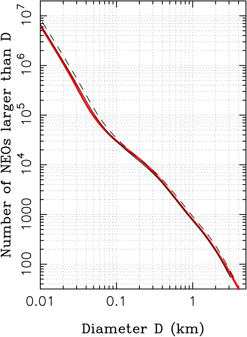
Figure 6: The size distribution of NEOs from our simple model (red line; Sects. 3.5 and 3.8) is compared to the size distributions constructed from the best-fit absolute magnitude distribution in Paper II and reference visual albedo $p_{\rm V}=0.14$ (dashed line) and 0.17 (solid line). The albedo distribution of NEOs used here comes from a global fit to the NEOWISE data. It is held constant over the whole range of diameters shown in the plot.

We used the method described in Sect. 3.8 to determine the size distribution of NEOs (Fig. 6). The best-fit size distribution is represented by splines in six diameter segments (Table 2). We find a relatively steep slope for $D<50$ m ($\beta\simeq 2.5$–2.8) and a bending, concave profile for $D>100$ m. We estimate $\simeq 6.5\times 10^{6}$ NEOs with $D>10$ m, $\simeq 30,\!000$ NEOs with $D>100$ m, and $\simeq 780$ NEOs with $D>1$ km. These estimates were obtained from the global (simple) fit where the albedo distribution was held constant over the whole range of diameters.

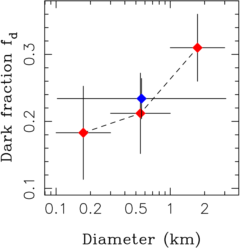
Figure 7: The fraction of NEOs in the dark Rayleigh peak ($f_{\rm d}$; Sect. 3.3) obtained from different MultiNest fits. The blue symbol and the errors bars show results from the global (simple) fit to all NEOWISE observations. The red symbols and the errors bars show results for fits in different size ranges. The dashed lines indicate the interpolated values used in the model with the size-dependent albedo distribution.

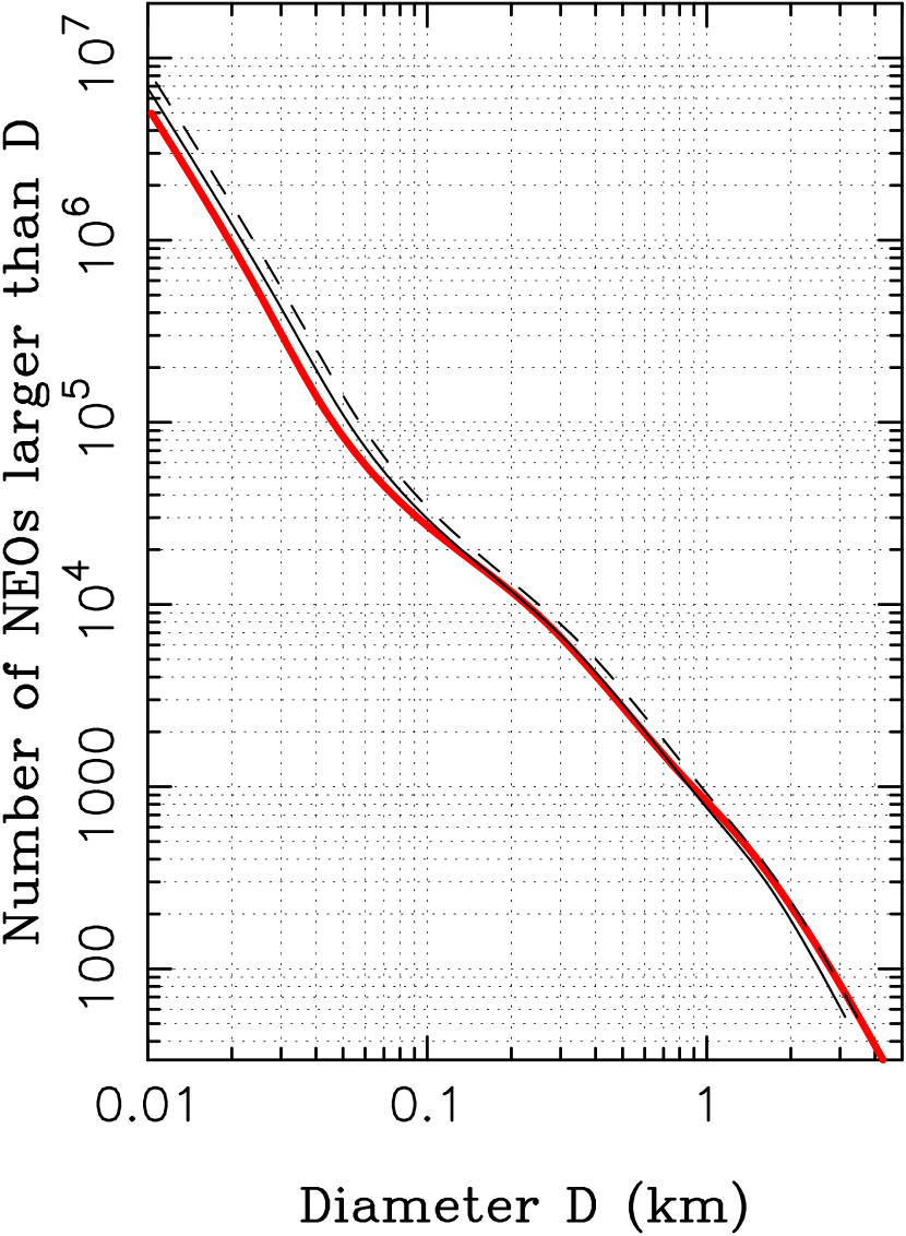
Figure 8: The size distribution of NEOs from our size-dependent albedo model (red line) is compared to the size distributions constructed from the best-fit absolute magnitude distribution in Paper II and reference visual albedo $p_{\rm V}=0.14$ (dashed line) and 0.17 (solid line). The size-dependent albedo distribution adopted here was constructed with the methods described in Sect. 4.1.

We also considered cases with the size-dependent albedo distribution, $\phi=\phi(p_{\rm V};D)$. The motivation for this comes from the NEOWISE data. For example, the mean albedo of NEOs computed from all cryogenic NEOWISE measurements is $\langle p_{\rm V}\rangle=0.165$. If the NEOWISE detections are split according to object’s size, however, we find that the mean albedo for $D>1$ km is $\langle p_{\rm V}\rangle=0.135$ and the mean albedo for $D<1$ km is $\langle p_{\rm V}\rangle=0.182$, suggesting some dependence of albedo on size. To test the possible size dependence, simple MultiNest fits were performed for NEOs of different sizes. We found, indeed, that the parameters $f_{\rm d}$, $d$ and $b$ change with size (Fig. 7). The results of these fits were interpolated to obtain $\phi(p_{\rm V};D)$. The size distribution was then constructed with $\phi(p_{\rm V};D)$ (Fig. 8). Table 3 reports our best estimates for the number of NEOs for the size-independent and size-dependent albedo distributions.

Our estimates are subject to several uncertainties: (1) We used the absolute-magnitude distribution from NEOMOD2 where the dominant source of error – at least for $H<25$ (CSS debiasing may have introduced additional errors for $H>25$) – was statistical in nature. In Paper II we estimated that this represented the relative uncertainty of $\simeq 3$% for $H<25$. (2) There is an important and potentially systematic uncertainty related to the absolute magnitude values reported in the Minor Planet Center (MPC) catalog (Pravec et al. 2012, Harris & Chodas 2023). As we discussed in Paper II, due to shifting magnitude values, the number of known NEOs with $H<17.75$ reported by MPC decreased by 49 from October 19, 2022 (our MPC download for Paper II) and March 13, 2023 (MPC download from Harris & Chodas 2023). If this trend holds, the number of $D>1$ km NEOs would be substantially revised. (3) Finally, there is the uncertainty arising from the albedo distribution of NEOs. From the simple MultiNest fits reported here, we conservatively estimate that the associated uncertainty is $<10$% for $D>100$ m (Table 3).

Accounting for items (1) and (3), we estimate $830\pm 60$ NEOs with $D>1$ km and $20,\!000\pm 2,\!000$ NEOs with $D>140$ m. These are the values quoted in the abstract and conclusions. The ranges given here contain all estimates from different models reported in Table 3, and include the complex model results described in Sect. 4.2. This is a conservative approach, because the differences between different model results are generally larger than statistical uncertainties of individual models. See Paper II for a method that can be used to rescale these estimates from item (2).

Related to the NASA goal to discover 90% of $D>140$ m NEOs, Fig. 9 shows the absolute magnitude distribution for $D>140$ m NEOs. We used the NEOMOD Simulator and generated all model NEOs with $D>140$ m. The results are plotted as a cumulative distribution of $H$ in Fig. 9. The distribution can be understood to indicate the fraction of $D>140$ m NEOs having magnitudes brighter than $H$. This information is relevant for the future telescopic surveys such as the Legacy Survey of Space and Time (LSST) of the Vera C. Rubin Observatory. For example, to reach a 90% completion for $D>140$ m, telescopic observations would need to detect all NEOs brighter than $H=22.2$ or $>90$% of NEOs brighter than $H=24$. For reference, the current completness for $H<22$ and $H<24$ is only $\simeq 35$% and $\simeq 10$%, respectively (Paper II).

4.2 Complex fits

While the simple models described in the previous section can be used to infer the albedo dependence on size, they cannot account for any albedo variation with orbit. There is some evidence in the NEOWISE data that the albedo distribution can be orbit dependent. For example, NEOs with $D>1$ km and $p_{\rm V}<0.1$ represent only $\simeq 40$% of all NEOs with $D>1$ km for $a<2$ au, but $\simeq 56$% for $a>2$ au, suggesting that the fraction of dark NEOs increases with the semimajor axis (Fig. 3). This trend is expected because NEOs should reflect the taxonomic distribution of asteroids in the main belt, where dark (C-complex) bodies become more common with increasing semimajor axis (DeMeo et al. 2009, Mainzer et al. 2019, Marsset et al. 2022). This motivates us to consider the complex MultiNest fits from Sect. 3.6, where individual main belt sources can have different contributions to dark and bright NEOs.

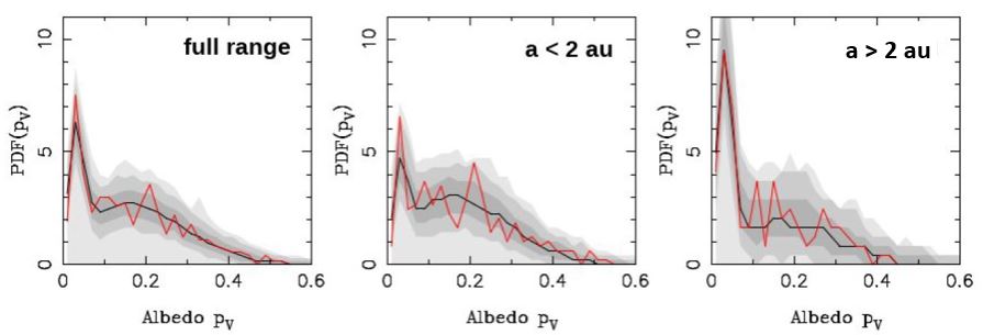
Figure 12: The (biased) albedo distribution from the complex model is compared to NEOWISE detections. From left to right the panels show the results for: (a) the full semimajor axis range, (b) $a<2$ au, and (c) $a>2$ au. For $a>2$ au, the dark peak of the albedo distribution is prominent. For $a<2$ au, the dark peak is subdued, indicating that NEOs with $a<2$ au more often have higher albedos. This happens because the inner belt sources have larger contributions to bright NEOs than the outer belt sources. The model correctly reproduces the dependence of the albedo distribution on the semimajor axis.

Table 4 and Fig. 10 report model parameters from the complex MultiNest fit. The complex model matches the NEOWISE data better than our simple model. The statistical preference for a model is given by the Bayes factor evaluated by MultiNest. We obtain $\Delta\ln{\cal Z}=15.9$, indicating a strong preference for the complex model. This can be readily understood because the complex model correctly emulates both the albedo dependence on size (Fig. 11) and orbit (Fig. 12). The fraction of dark NEOs ($p_{\rm V}<0.1$) is found to increase with the semimajor axis. This is expected because dark (C-complex) asteroids are more common near NEO sources in the outer main belt. For $1<a<2$ au the fraction of NEOs with $p_{\rm V}<0.1$ is $25\pm 15$%; it increases to $65\pm 15$% at $a\sim 3$ au.

The NEOWISE data do not provide sufficint information to constrain all (complex) model parameters. For example, the posterior distribution for $f_{{\rm d},j}$ parameters corresponding to 7:3, 9:4 and comets is nearly uniform between 0 and 1 (Fig. 10). This happens because these sources do not have a significant contribution to NEOs anyway (NEOMOD2 only gives a $<2$% contribution for them; Paper II). In some cases, such as Hungarias, we only obtain an upper bound with $f_{\rm d}<22$%. In other cases, such as the 11:5 resonance, we obtain a lower bound with $f_{\rm d}>72$%. The upper (lower) limits mean that the low-albedo (high-albedo) bodies should represent the great majority of NEOs produced from that source.

In general, the contribution of sources to dark NEOs correlates with the semimajor axis. The inner belt sources such as $\nu_{6}$ and 3:1 have low contributions, and the outer belt sources such as 11:5 and 2:1 have high contributions (Fig. 13). A similar trend was reported in Morbidelli et al. (2020). As in Morbidelli et al. (2020), here we also find a relatively large contribution to dark NEOs from Phocaeas ($\simeq 50$% for $p_{\rm V}<0.1$ in Morbidelli et al. and $>65$% for $p_{\rm V}<0.1$ here). This is inconsistent with other observational evidence which suggests that Phocaeas are mostly bright (S-type) asteroids (DeMeo et al. 2009; about 1/3 of Phocaeas have $p_{\rm V}<0.1$, Mainzer et al. 2019). The problem may arise from the relatively low statistics of NEOWISE detections: a handful of dark NEOs were detected by NEOWISE on high-inclination orbits where the Phocaea source is expected to contribute. Either that, or we are missing a source of dark NEOs on high inclination orbits.

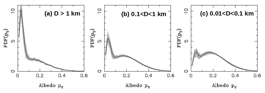
Figure 14: The debiased albedo distribution of NEOs from the complex model. From left to right the panels show the results for: (a) $D>1$ km, (b) $0.1<D<1$ km, and (c) $0.01<D<0.1$ km. For $D>1$ km, the dark peak of the albedo distribution is prominent. For $D<0.1$ km, the dark peak is subdued indicating that small NEOs are more often found in the peak with higher albedos. The mean albedos for the three size ranges shown here are $\langle p_{\rm V}\rangle=0.124$ ($D>1$ km), 0.167 ($0.1<D<1$ km) and 0.191 ($0.01<D<0.1$ km).

Figure 14 illustrates the size-dependent albedo distribution of NEOs from the debiased complex model. The distributions shown here for $D>0.1$ km are in good agreement with those obtained with different size cuts in the simple model (Sect. 4.1). For $1<D<3$ km, the complex model indicates $f_{\rm d}=0.33$, in a close match to the result reported in Fig. 7. For $0.1<D<0.3$ km, we have $f_{\rm d}=0.23$, slightly higher than $f_{\rm d}=0.18$ from the simple model. Some differences are expected given the different schemes employed in our simple and complex models. The albedo distribution for $D<0.1$ km is an extrapolation with NEOMOD2 and the complex model parameters listed in Table 3. If these results are correct, the importance of the dark Rayleigh peak continues to diminish for $D<0.1$ km, indicating that (very) small NEOs are on average (much) brighter than large NEOs.

The complex model inferences for the size distribution of NEOs are consistent with those obtained from the simple model. Because the $f_{\rm d}$ values tend to be slightly larger in the complex model, here we obtain slightly higher population estimates than $N_{3}(D)$ reported in Table 3, nominally 873 NEOs with $D>1$ km and 19,500 NEOs with $D>140$ m. This is well within the range of uncertainties discussed in Section 4.1. The population estimates from the complex model could be favored over those obtained in the simple model, because the complex model is more successful in reproducing various orbital dependences. In some cases, however, such as the Phocaea case discussed above (also see Morbidelli et al. 2020), the inferences obtained from the complex model are somewhat uncertain. In this situation, we prefer to report the full range of population estimates from the simple and complex models. This is why the abstract and conclusions give $830\pm 60$ NEOs with $D>1$ km and $20,\!000\pm 2,\!000$ NEOs with $D>140$ m.

The reference albedo value $p_{\rm V,ref}$ for an approximate conversion of the absolute magnitude distribution to the size distribution (e.g., Harris & Chodas 2021) is a function of absolute magnitude. We recommend $p_{\rm V,ref}\simeq 0.15$ for $H<18$, $p_{\rm V,ref}\simeq 0.16$ for $18<H<22$, and $p_{\rm V,ref}\simeq 0.18$ for $H>22$.

5 Discussion

5.1 Simple vs. complex model inferences

There are at least two obvious biases in NEOWISE observations. The first one is the thermal infrared bias discussed in Section 3.2 (objects with low visual albedo emit more thermal radiation and are more easily detected in infrared wavelengths). Our simple model rigorously accounts for the thermal bias (Sect. 3.5). The second one is the orbital bias: the NEOWISE data set is biased toward detection of NEOs with small heliocentric distances. These NEOs are warmer and more easily detected in thermal infrared. We know that NEOs at small heliocentric distances predominantly sample sources in the inner asteroid belt; they are more likely to have higher albedos than NEOs on larger orbits. This means that NEOWISE is biased toward higher albedos. This is not something we can account for in the simple model. The simple model calibrates the albedo distribution on NEOs detected by NEOWISE (the thermal bias is accounted for) and adopts it for NEOs in general. The simple model should thus be biased toward higher albedos as well (due to the orbital bias).

The debiased albedo distribution obtained from the complex model does not suffer from this limitation, at least not as much as the simple model, because it adopts the orbital distribution of NEOs from NEOMOD2. For example, the $\nu_{6}$ resonance produces evolved NEOs with $a<2$ au. These bodies escape from the inner asteroid belt and often have $p_{V}>0.1$. The $\nu_{6}$ resonance is thus assigned a relatively low value of the parameter $f_{\rm d}$, and the albedo distribution – specific for the $\nu_{6}$ resonance – is then extended with a proper weight to the whole NEO population.

The same applies to other sources as well. So, at least in principle, the complex model should give us a more realistic albedo distribution of NEOs, including its proper scaling with size and orbit. This may explain some of the differences discussed in Sect. 4.2. Note that these differences are not large, however, suggesting that the orbital bias in the simple model is not overwhelmingly important. We discuss the simple model in this work because the simple model is firmly tied to NEOWISE observations, does not require additional assumptions (e.g., related to how NEOs sample various main belt sources), and allows us to test the albedo dependence on size. The fact that the simple and complex models lead to consistent results is reassuring.

Additional uncertainties arise because even the complex model does not account for the possibility that the albedo distribution of NEOs from source $j$ can be size-dependent (e.g., because the low- and high-albedo main-belt asteroids near that source have different size distributions). The model defines the albedo distribution from source $j$ as unchanging with size, and injects the size and orbit dependence of NEO albedo via the size-dependent contribution of sources, $\alpha_{j}(H)$ (Paper II). Investigations into more complete albedo models are left for future work.

5.2 Relationship to main belt asteroids

Some features of the complex model seem surprising. For example, according to Fig. 13, the $\nu_{6}$ resonance is inferred to produce only $\simeq 20$% of NEOs with $p_{\rm V}<0.1$. If we look in the immediate neighborhood of the $\nu_{6}$ resonance in the main belt, we find that $\simeq 40$% of asteroids with $1<D<2$ km have $p_{\rm V}<0.1$ (Mainzer et al. 2019). This can mean one of several things. In NEOMOD2, the $\nu_{6}$ source does not have much contribution to NEOs with $D>1$ km (Paper II). The albedo distribution of $\nu_{6}$ is thus mainly calibrated on small, sub-km NEOs detected by NEOWISE. Since these small bodies were not detected by NEOWISE in the main belt, however, we cannot be sure that there really is a problem. A similar argument applies to the 3:1 resonance as well.

In more general terms, we find here that dark NEOs with $p_{\rm V}<0.1$ represent $\simeq 40$% of the NEO population (for $D\sim 1$ km). This is lower than the share of dark asteroids in the main belt ($\sim 60$% overall from WISE; Mainzer et al. 2019). The difference is in part caused by how NEOs sample the main belt – they preferentially come from the inner part of the belt where dark asteroids are less common. Overall, dark bodies with $p_{\rm V}<0.1$ contribute to $\sim 40$% of asteroids in the inner belt (2–2.5 au). The NEOWISE data also indicate that the albedo distribution of inner belt asteroids may be size dependent. For example, dark bodies with $p_{\rm V}<0.1$ represent 55% of inner belt asteroids with $D>10$ km, but only 27% of inner belt asteroids with $1<D<2$ km.

5.3 NEO population estimates

We estimate $830\pm 60$ NEOs with diameters $D>1$ km and $30,\!000\pm 3,\!000$ NEOs with $D>100$ m (Table 3). This can be compared to $\simeq 20,\!500\pm 3000$ NEOs with $D>100$ m and $981\pm 19$ NEOs with $D>1$ km reported in Mainzer et al. (2011), and $\sim 1000$ NEOs with $D>1$ km in Morbidelli et al. (2020). Our population estimate for $D>100$ m is $\sim 50$% higher. We believe that our method better approximates the debiased size distribution for $D<1$ km. Our estimate for $D>1$ km is $\sim 15$% lower. We think that this happens because Mainzer et al. (2011) used an approximate Monte Carlo method to infer the number of large NEOs. Here we infer it by inverting Eq. (12), which is a more rigorous approach.

The error estimates reported here combine various uncertainties related to our inferences about the absolute magnitude distribution from NEOMOD2 and the albedo distribution from NEOWISE. We find that the dominant source of error - at least the one that we are able to characterize at the present time - reflects uncertainties in the albedo distribution of NEOs. As we varied the debiasing method and tweaked parameters in the MultiNest fits, we found that the estimates vary by $\lesssim 10$%. Hence our conservative error estimates, but note that systematic changes of MPC magnitudes are not accounted for here (see Sect 4.1).

5.4 Impact flux on the Earth

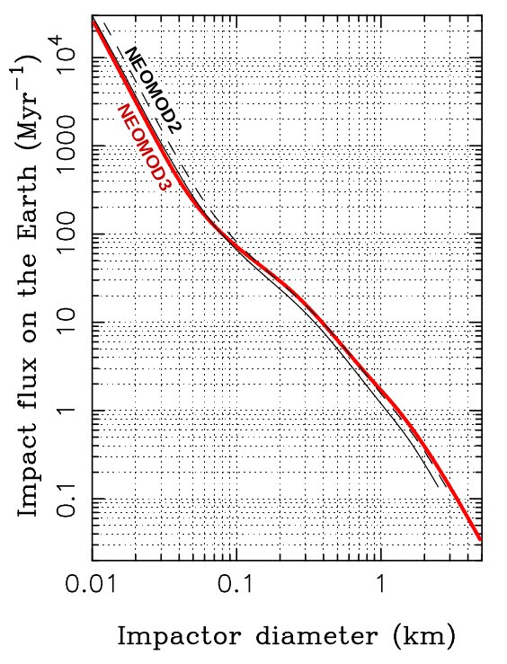
Figure 15: The impact flux of NEOs on the Earth from our model with the size-dependent albedo distribution (red line). The size-dependent albedo distribution model adopted here was constructed with the methods described in Sect. 4. The impact flux from NEOMOD2 is plotted for reference. For that we used $p_{\rm V}=0.14$ (dashed black line) and $p_{\rm V}=0.18$ (solid black line) to translate the absolute magnitudes from NEOMOD2 to diameters.

Here we estimate the impact flux of NEOs on the Earth. This is done by combining the absolute magnitude distribution from NEOMOD2, the albedo distribution from NEOWISE, and the intrinsic impact probability, $P_{\rm i}(H)$, for NEO impacts on the Earth from Paper II. The impact flux is obtained by inverting Eq. (12), where instead of $\psi(D)$ in the integrand there is $P_{\rm i}(H)\psi(D)$. For reference, $P_{\rm i}=1.53\times 10^{-3}$ Myr^-1 for $H=15$, $P_{\rm i}=2.1\times 10^{-3}$ Myr^-1 for $H=20$ and $P_{\rm i}=2.6\times 10^{-3}$ Myr^-1 for $H=25$ (Paper II). Figure 15 shows the impact flux for the size-dependent albedo model, including the tidal disruption model from Paper II. Table 5 reports the number of impacts for several reference impactor diameters.

We estimate 1.51–1.74 impacts/Myr of $D>1$ km NEOs on the Earth. The average interval between impacts of $D>1$ km is 570–660 kyr. This is shorter than the estimate given in Morbidelli et al. (2020) who found the average interval $\simeq 750$ kyr. The difference reflects different population estimates and different impact probabilities adopted in these works. For $D>140$ m, we find 42–52 impacts/Myr and the average interval between impacts 19–24 kyr. We can also compare our results with Nesvorný et al. (2021), where a different method was used for very large NEOs. They inferred 16–32 impacts/Gyr of $D>5$ km NEOs on the Earth. Here we find $\sim 30$ such impacts (Fig. 15), a value near the upper end of the range given in Nesvorný et al. (2021). The trend pointed out here, with the larger share of dark bodies among large NEOs is consistent with Nesvorný et al. (2021), who argued that dark (primitive) asteroids represent about a half of very large impactors ($D\gtrsim 5$ km) on the Earth.

For the smallest impactors shown in Fig. 15, we find that the mean interval between impacts of $D>10$ m NEOs is $\sim 40$ years. This is consistent with the results reported in Paper II (see the black solid line in Fig. 15) given that the results presented here suggests that the albedo of small NEOs should be relatively high - effective $p_{\rm V}\simeq 0.18$ (instead of the usual reference $p_{\rm V}=0.14$, Paper II). This is a consequence of the $\nu_{6}$ resonance having a relatively large contribution for small and bright NEOs. The impact flux obtained here is a factor of $\sim 4$ below the impact flux estimate obtained from bolide observations ($\sim 10$ yr interval between impacts of $D>10$ m NEOs; Brown et al. 2013), which is a problem.

The visible albedos of $D\sim 10$ m NEOs obtained in this work may be too high. The albedo distribution of small, $D<100$ m NEOs was obtained here by calibrating the model on relatively large NEOs ($D>100$ m) detected by NEOWISE. In the complex model, we assumed that the number ratio of dark over bright bodies, as calibrated for individual sources on $D>100$ m NEOs, does not change for $D<100$ m. This assumption may be incorrect. For example, the contribution of dark asteroid families close to the $\nu_{6}$ and/or 3:1 sources may be insignificant for $D>100$ m, but important for $D<100$ m. If so, this would effectively lower the reference albedo. Another possibility is that the tidal disruption of NEOs during close planetary encounters (Paper II) disproportionally affects dark NEOs, perhaps because they are weak, and creates an excess of small dark NEOs on orbits with high impact probabilities on the Earth (this effect is not taken into account in the present work).

5.5 Lunar production function

The radiometric ages, crater counts and size distribution extrapolations are the basis of empirical models for impact cratering in the inner solar system (see Ivanov et al. 2002 for a review). The standard approach to this problem is to conduct crater counts on different lunar terrains and patch them together to estimate the lunar production function (LPF), defined as the number of craters larger than diameter $D_{\it crater}$ produced on 1 km² of the lunar surface in Gyr. Here we estimate the current-day LPF from the size distribution of NEOs (also see Marchi et al. 2009). The results shown in Fig. 15 are carried over to lunar impacts with the standard Earth-to-Moon ratio (${\cal R}=20$; Paper I). We adopt the crater scaling laws from Johnson et al. (2016), for which a $D=1$-km NEO impactor makes a $D_{\rm crater}\simeq 20$-km lunar crater, and a $D\simeq 40$-m NEO impactor makes a $D_{\rm crater}\simeq 1$ km lunar crater (see Morbidelli et al. (2018) for a discussion).

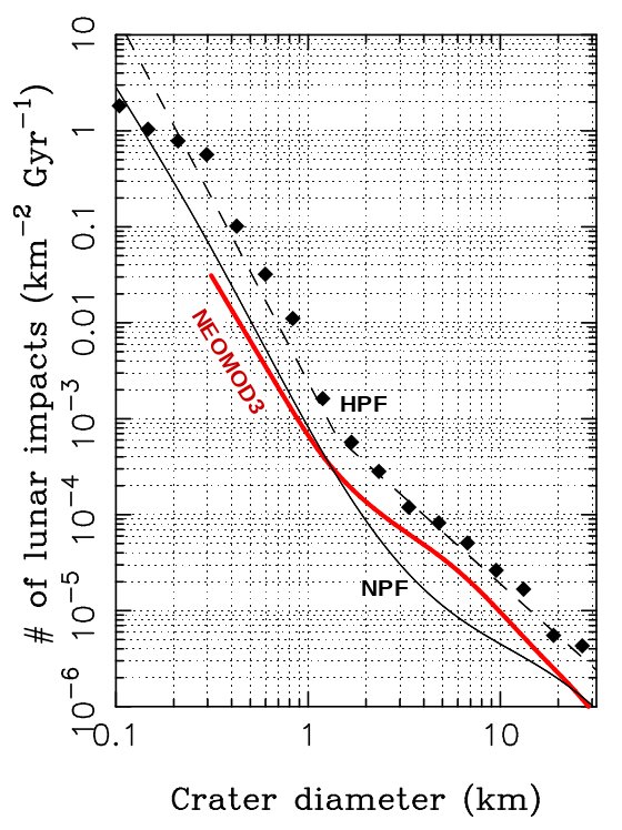
Figure 16: The lunar production function. The plot shows the cumulative distribution of crater diameters produced on the lunar surface in Gyr. The number of craters is normalized to 1 km² of the lunar surface. The red line is the production function obtained here from NEOMOD (Sect. 5.5). The black solid line is the Neukum’s production function (NPF) as reported in Table 1 in Ivanov et al. (2002) (the column “New” $N(D)$, Neukum et al. 2001). The black diamonds are the Hartmann’s production function (HPF) from Hartmann (1995). Finally, the dashed line is the piece-wise power-law fit to HPF as given in Eqs. (1a)-(1c) in Ivanov et al. (2002).

Figure 16 compares our LPF with those inferred from the crater counts in Hartmann (1995) and Neukum et al. (2001). This is not a one-to-one comparison for several different reasons. For example, the lunar craters with $D_{\rm crater}<1$ km are often secondaries (i.e., craters formed by re-impacting material ejected from a primary crater; Bierhaus et al. 2018). The secondaries are not accounted for in our model. Also, there are not enough large craters with $D_{\rm crater}\gtrsim 10$ km on the young lunar terrains – the empirical LPF for $D_{\rm crater}\gtrsim 10$ km must therefore be inferred from old lunar terrains, but the old lunar terrains may have seen impactor populations other than modern NEOs (Nesvorný et al. 2022, 2023b).

With these caveats in mind, we find that our LPF is roughly intermediate between LPFs reported in Hartmann (1995) and Neukum et al. (2001) (Fig. 16). For $D_{\rm crater}<1$ km, the empirical LPFs are somewhat steeper than our LPF possibly due to the contribution of secondaries (secondary craters tend to have steep size distributions; Bierhaus et al. 2018). For some reason, our LPF runs below that of Hartmann (1995), indicating a problem with the absolute calibration, but nicely reproduces the slope transition near $D_{\rm crater}=1.5$ km (steeper for $D_{\rm crater}<1.5$ km, shallower for $D_{\rm crater}>1.5$ km). Neukum’s LPF shows a broader transition near $D_{\rm crater}=5$ km, but the shape of this transition may be affected by crater counts on very old lunar terrains.

6 Conclusions

The main results of this work are summarized as follows:

(1) We developed approximate methods to debias the albedo distribution of NEOs detected by NEOWISE. The debiased albedo distribution can be accurately described by a sum of two Rayleigh distributions representing NEOs with low ($p_{\rm V}\lesssim 0.1$) and high albedos ($p_{\rm V}\gtrsim 0.1$).

(2) There is good evidence that the albedo distribution of NEOs is size and orbit dependent. Smaller NEOs tend to have higher albedos than large NEOs. NEOs with evolved orbits below 2 au tend to have higher albedos than NEOs beyond 2 au.

(3) The debiased albedo distribution and absolute magnitude distribution of NEOs from NEOMOD2 (Paper 2) were used to infer the size distribution of NEOs. We estimate $830\pm 60$ NEOs with diameters $D>1$ km and $20,\!000\pm 2,\!000$ NEOs with $D>140$ m. See the bold paragraph in Sect. 4.1 for how these estimates and their uncertainities were synthesized from different models (the range contains estimates from all models investigated here).

(4) The reference albedo value $p_{\rm V,ref}$ for an approximate conversion of the absolute magnitude distribution to the size distribution is a function of absolute magnitude. We recommend $p_{\rm V,ref}\simeq 0.15$ for $H<18$, $p_{\rm V,ref}\simeq 0.16$ for $18<H<22$, and $p_{\rm V,ref}\simeq 0.18$ for $H>22$.

(5) The intrinsic impact probability from NEOMOD2 was combined with the population estimates obtained here to infer the impact rates of NEOs on the Earth. We estimate the average interval between impacts of $D>1$ km NEOs about 640 kyr, and the average interval between impacts of $D>140$ m NEOs about $20,\!000$ yr.

(6) We used the NEO model to estimate the production function of lunar craters. The lunar production function (LPF) is found to have an inflection point for $D_{\rm crater}\simeq 1.5$ km, with the steeper slope for $D_{\rm crater}<1.5$ km and shallower slope for $D_{\rm crater}>1.5$ km. A similar slope transition was inferred from the lunar crater counts in Hartmann (1995).

(7) The upgraded model, NEOMOD3, is available via the NEOMOD Simulator – a user-friendly code that can be used to generate samples (orbits, sizes and albedos of NEOs) from the model.

7 Appendix A: Albedo bias in visible surveys

Assume, for example, a bimodal (differential) distribution of albedos, $\phi(p_{\rm V})={\rm d}N/{\rm d}p_{\rm V}$, with $\phi_{\rm dark}(p_{\rm V})=\delta(p_{\rm V}-d)$ for dark objects and $\phi_{\rm bright}(p_{\rm V})=\delta(p_{\rm V}-b)$ for bright objects, where $\delta$ are delta functions, and $b$ and $d$ are some characteristic albedo values of dark and bright objects, respectively. For example, Wright et al. (2016) found that the albedo distribution of NEOs detected by NEOWISE can be approximated by a sum of two Rayleigh distributions with the scale factors $d=0.03$ and $b=0.168$. Assume, in addition, that the size distributions of dark and bright objects, $\psi(D)={\rm d}N/{\rm d}D$, can be approximated by the same power law slope, $\psi_{\rm dark}(D)=f_{\rm d}N_{0}D^{-\alpha}$ for dark and $\psi_{\rm bright}(D)=(1-f_{\rm d})N_{0}D^{-\alpha}$ for bright, where $f_{\rm d}$ is the share of dark objects in the population, and $\alpha$ is fixed.

The (differential) magnitude distribution, $n(H)={\rm d}N/{\rm d}H$, can be obtained by evaluating the integral over all albedo values

$$n(H)={1\over\kappa}\int_{0}^{1}\,{\rm d}p_{\rm V}\,\phi(p_{\rm V})D\psi(D)\ ,$$ (13)

where $\kappa=-5/\ln 10$, $D=D(H,p_{\rm V})=c10^{-H/5}/\sqrt{p_{\rm V}}$, and $c=1329$ km. For the example discussed above, this gives $n(H)=N^{\prime}_{0}10^{\gamma H}$ with $\gamma=(\alpha-1)/5$, $N^{\prime}_{0}=N_{0}c^{-5\gamma}p_{\rm V,ref}^{5\gamma/2}/\kappa$, and the reference albedo $p_{\rm V,ref}^{5\gamma/2}=f_{\rm d}d^{5\gamma/2}+(1-f_{\rm b})b^{5\gamma/2}$. The reference albedo $p_{\rm V,ref}$ can be used to convert the absolute magnitude distribution to the size distribution. The real absolute magnitude distribution of NEOs is wavy (Figure 2) with $\gamma\simeq 0.3$–0.55 (Papers I and II). For $\gamma=0.4$, we have $5\gamma/2=1$ and the reference albedo is just a normal (weighted by $f_{\rm d}$) mean of $d$ and $b$. For the example from Wright et al. (2016), with $d=0.030$ and $b=0.168$, this gives $p_{\rm V,ref}=0.133$. For $\gamma=0.3$ and 0.5, we have $p_{\rm V,ref}=0.128$ and $p_{\rm V,ref}=0.137$, respectively.

Now, as for the albedo bias in a visual-magnitude limited survey, the sizes of the dark and bright objects with the same magnitude $H$ are $D_{\rm d}=c10^{-H/5}/\sqrt{d}$ and $D_{\rm b}=c10^{-H/5}/\sqrt{b}$. The fraction of dark objects in a magnitude-limited survey is then $f^{\prime}_{\rm d}=f_{\rm d}D_{\rm d}^{-\alpha}/[f_{\rm d}D_{\rm d}^{-\alpha}+(1-f_{\rm d})D_{b}^{-\alpha}]$. This gives

$$f^{\prime}_{\rm d}=f_{\rm d}\left[f_{\rm d}+(1-f_{\rm d})\left({b\over d}\right)^{\alpha/2}\right]^{-1}\ .$$ (14)

For the example discussed above with $f_{\rm d}=0.253$ and $\gamma=0.4$, we have $\alpha=3$ and $f^{\prime}_{\rm d}=0.025$. So, the bright objects would represent 97.5% of all objects (even though their actual share in a size-limited sample is only 74.7%). Additional complications would arise if the dark and bright objects do not have the same power slope index or if the power slope index changes with size.

In more general terms, $\phi(p_{\rm V})$ from Eq. (10) and $\phi^{\prime}(p_{\rm V})$ from Eq. (11) are related via

$$\phi^{\prime}(p_{\rm V};H)=C_{\rm N}{D\over\kappa}\psi(D)\phi(p_{\rm V};D)\ ,$$ (15)

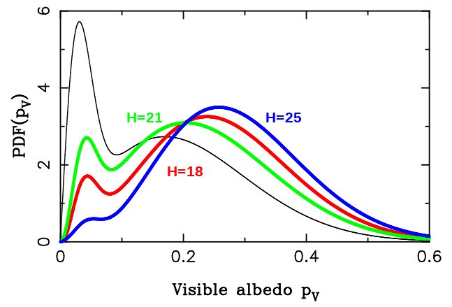
Figure 17: The albedo distribution from our simple model, $\phi(p_{\rm V})$ (black line; Eq. (10), Table 1) is compared to the albedo distributions, $\phi^{\prime}(p_{\rm V};H)$ (Eq. 11), for $H=18$ (red line), $H=21$ (green line) and $H=25$ (blue line). The difference between $\phi$ (size-based distribution) and $\phi^{\prime}$ (absolute-magnitude-based distribution) is the largest for $H=25$, where the absolute magnitude distribution has the steepest slope (Fig. 2).

again with $\kappa=-5/\ln 10$, $D=D(H,p_{\rm V})=c10^{-H/5}/\sqrt{p_{\rm V}}$, and $c=1329$ km. The right-hand side of Eq. (15) is to be evaluated for a fixed value of $H$. The normalization constant $C_{\rm N}$ assures that $\int{\rm d}p_{\rm V}\phi^{\prime}(p_{\rm V};H)=1$ for any $H$ (also, by definition, $\int{\rm d}p_{\rm V}\phi(p_{\rm V};D)=1$ for any $D$). For a bimodal albedo distribution with $\phi(p_{\rm V})$ being represented by delta functions and a single power-law size distribution $\psi(D)$, Eq. (15) can be reduced to the arguments discussed above. Figure 17 illustrates a more general case where we adopt (size-independent) $\phi(p_{\rm V})$ from our simple model, the size distribution of NEOs shown in Fig. 6, and compute $\phi^{\prime}(p_{\rm V};H)$ from Eq. (15) for several different values of the absolute magnitude. The plot illustrates the difference between different definitions of albedo distribution.

label	parameter	median	$-\sigma$	$+\sigma$
(1)	$f_{\rm d}$	0.233	0.028	0.030
(2)	$d$	0.029	0.003	0.003
(3)	$b$	0.170	0.006	0.006

Table 1: The median and uncertainities of our simple (global) model parameters (Sect. 3.5). The first column is the parameter/plot label in Fig. 4. The uncertainties reported here were obtained from the posterior distribution produced by MultiNest.

parameter	$D$ range	value	$D$ range	value
	(km)		(km)
	constant albedo model		variable albedo model
$N_{\rm ref}$	–	$777\pm 24$	–	$813\pm 24$
$\beta_{1}$	0.001–0.028	$2.54\pm 0.03$	0.001–0.026	$2.53\pm 0.03$
$\beta_{2}$	0.028–0.044	$2.73\pm 0.03$	0.026–0.041	$2.75\pm 0.03$
$\beta_{3}$	0.044–0.278	$1.50\pm 0.02$	0.041–0.261	$1.50\pm 0.02$
$\beta_{4}$	0.278–0.876	$1.85\pm 0.03$	0.261–0.824	$1.72\pm 0.02$
$\beta_{5}$	0.876–1.389	$1.86\pm 0.06$	0.824–1.306	$1.66\pm 0.05$
$\beta_{6}$	1.389–30.00	$2.63\pm 0.09$	1.306–30.00	$2.58\pm 0.09$

Table 2: The normalization parameter ($N_{\rm ref}$) and cumulative slopes ($\beta_{j}={\rm d}\log N/{\rm d}\log D$) from our (debiased) size distribution models of NEOs. The constant albedo model was obtained from the global (simple) fit to all NEOWISE data. The variable (i.e., size-dependent) albedo model was constructed from fits in different size ranges (Sect. 4.1). The parameter $N_{\rm ref}$ calibrates the size distribution for $D>1$ km. Note that the actual size distribution is computed from cubic splines that smoothly connect the slopes in different segments (Figs. 6 and 8). The number of $D>1$ km NEOs is thus (slightly) larger than $N_{\rm ref}$ (Paper I).

	$N_{1}(D)$	$N_{2}(D)$	$N_{3}(D)$
$D>1$ km	779	891	828
$D>300$ m	7330	8208	6620
$D>140$ m	20,000	22,100	18,000
$D>100$ m	30,200	33,500	27,000
$D>30$ m	368,000	427,000	307,000

Table 3: The estimated number of NEOs, $N(D)$, larger than diameter $D$. In the second column, $N_{1}(D)$ stands for the estimates obtained from the global (simple) model to all NEOWISE data. In the third column, $N_{2}(D)$ is based on the fixed albedo model obtained for $1<D<3$ km and used for all NEOs. In the forth column, $N_{3}(D)$ corresponds to the variable albedo model constructed with the methods described in Sect. 4.1. The range of estimates given here roughly expresses the uncertainty related to the albedo distribution. The ranges given in the abstract and conclusions, $830\pm 60$ NEOs with $D>1$ km and $20,\!000\pm 2,\!000$ NEOs with $D>140$ m, conservatively contain different estimates from all models presented here, including the complex model results from Sect. 4.2.

label	parameter	median	$-\sigma$	$+\sigma$	limit
(1)	$f_{\rm d}(\nu_{6})$	0.037	0.025	0.044	0.054
(2)	$f_{\rm d}($3:1)	0.069	0.048	0.080	0.103
(3)	$f_{\rm d}($5:2)	0.247	0.165	0.232	–
(4)	$f_{\rm d}($7:3)	0.498	0.329	0.334	–
(5)	$f_{\rm d}($8:3)	0.721	0.217	0.173	–
(6)	$f_{\rm d}($9:4)	0.498	0.334	0.336	–
(7)	$f_{\rm d}($11:5)	0.814	0.204	0.129	0.723
(8)	$f_{\rm d}($2:1)	0.599	0.193	0.179	–
(9)	$f_{\rm d}($inner)	0.335	0.156	0.159	–
(10)	$f_{\rm d}($Hun)	0.149	0.104	0.169	0.222
(11)	$f_{\rm d}($Pho)	0.761	0.170	0.143	–
(12)	$f_{\rm d}($comets)	0.463	0.308	0.342	–
(13)	$d$	0.027	0.002	0.003	–
(14)	$b$	0.172	0.006	0.006	–

Table 4: The median and uncertainities of our complex model parameters. The first column is the parameter/plot label in Fig. 10. The uncertainties reported here were obtained from the posterior distribution produced by MultiNest. For parameters, for which the posterior distribution shown in Fig. 4 peaks near zero, the last column reports the upper (68.3% of posteriors fall between zero and that limit) or lower limit (68.3% of posteriors fall between that limit and one).

	$I_{1}(D)$	$I_{2}(D)$	$I_{3}(D)$
	Myr-1	Myr-1	Myr-1
$D>1$ km	1.51	1.74	1.61
$D>300$ m	16.1	18.1	14.4
$D>140$ m	46.7	52.0	41.9
$D>100$ m	72.7	81.0	64.8
$D>30$ m	993	1160	829

Table 5: The impact flux of NEOs on the Earth, $I(D)$, for bodies larger than diameter $D$. In the second column, $I_{1}(D)$ stands for the estimates obtained from the global (simple) model to all NEOWISE data. In the third column, $I_{2}(D)$ is based on the fixed albedo model obtained for $1<D<3$ km and used for all NEOs. In the forth column, $I_{3}(D)$ corresponds to the variable albedo model constructed with the methods described in Sect. 4.1. The range of estimates given here roughly expresses the uncertainty related to the albedo distribution.

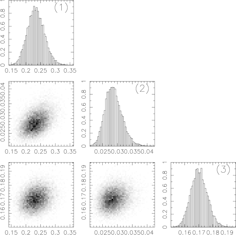
Figure 4: The posterior distribution of model parameters from our simple MultiNest fit (Sect. 3.5). The individual plots are labeled (1) to (3) following the model parameter sequence given in Table 1.

Figure 9: The fraction of diameter $D>140$ m NEOs having magnitudes brighter than $H$. To reach a 90% completion for $D>140$ m, telescopic observations in visible wavelengths would need to detect all NEOs brighter than $H=22.2$.

Figure 10: The posterior distribution of 14 model parameters from our complex MultiNest (Sects. 3.6). The individual plots are labeled (1) to (12) following the model parameter sequence given in Table 3.

Figure 13: The fraction of NEOs with $p_{\rm V}<0.1$ produced from each source. We used the $f_{{\rm d},j}$ parameters reported in Table 3 and summed up the contributions of dark and bright Rayleigh distributions from each source to $p_{\rm V}<0.1$.

References

- Bierhaus et al. (2018) Bierhaus, E. B. and 6 colleagues 2018. Secondary craters and ejecta across the solar system: Populations and effects on impact-crater-based chronologies. Meteoritics and Planetary Science 53, 638–671. doi:10.1111/maps.13057
- Bottke et al. (2002) Bottke, W. F. and 6 colleagues 2002. Debiased Orbital and Absolute Magnitude Distribution of the Near-Earth Objects. Icarus 156, 399–433. doi:10.1006/icar.2001.6788
- Brown et al. (2013) Brown, P. G. and 32 colleagues 2013. A 500-kiloton airburst over Chelyabinsk and an enhanced hazard from small impactors. Nature 503, 238–241. doi:10.1038/nature12741
- Christensen et al. (2012) Christensen, E. and 8 colleagues 2012. The Catalina Sky Survey: Current and Future Work. AAS/Division for Planetary Sciences Meeting Abstracts #44.
- DeMeo et al. (2009) DeMeo, F. E., Binzel, R. P., Slivan, S. M., Bus, S. J. 2009. An extension of the Bus asteroid taxonomy into the near-infrared. Icarus 202, 160–180. doi:10.1016/j.icarus.2009.02.005
- Feroz and Hobson (2008) Feroz, F., Hobson, M. P. 2008. Multimodal nested sampling: an efficient and robust alternative to Markov Chain Monte Carlo methods for astronomical data analyses. Monthly Notices of the Royal Astronomical Society 384, 449–463. doi:10.1111/j.1365-2966.2007.12353.x
- Feroz et al. (2009) Feroz, F., Hobson, M. P., Bridges, M. 2009. MULTINEST: an efficient and robust Bayesian inference tool for cosmology and particle physics. Monthly Notices of the Royal Astronomical Society 398, 1601–1614. doi:10.1111/j.1365-2966.2009.14548.x
- Granvik et al. (2016) Granvik, M. and 8 colleagues 2016. Super-catastrophic disruption of asteroids at small perihelion distances. Nature 530, 303–306. doi:10.1038/nature16934
- Granvik et al. (2018) Granvik, M. and 8 colleagues 2018. Debiased orbit and absolute-magnitude distributions for near-Earth objects. Icarus 312, 181–207. doi:10.1016/j.icarus.2018.04.018
- Harris (1998) Harris, A. W. 1998. A Thermal Model for Near-Earth Asteroids. Icarus 131, 291–301. doi:10.1006/icar.1997.5865
- Harris and D’Abramo (2015) Harris, A. W., D’Abramo, G. 2015. The population of near-Earth asteroids. Icarus 257, 302–312. doi:10.1016/j.icarus.2015.05.004
- Harris and Chodas (2021) Harris, A. W., Chodas, P. W. 2021 (HC21). The population of near-earth asteroids revisited and updated. Icarus 365. doi:10.1016/j.icarus.2021.114452
- Harris and Chodas (2023) Harris, A. W., Chodas, P. W. 2023. Update of NEA population and survey completion, ACM conference in Flagstaff, https://www.hou.usra.edu/meetings/acm2023/pdf/2519.pdf
- Hartmann (1995) Hartmann, W. 1995. Planetary cratering I: Lunar highlands and tests of hypotheses on crater populations. Meteoritics 30, 451. doi:10.1111/j.1945-5100.1995.tb01152.x
- Ivanov et al. (2002) Ivanov, B. A., Neukum, G., Bottke, W. F., Hartmann, W. K. 2002. The Comparison of Size-Frequency Distributions of Impact Craters and Asteroids and the Planetary Cratering Rate. Asteroids III 89–101.
- JeongAhn and Malhotra (2014) JeongAhn, Y., Malhotra, R. 2014. On the non-uniform distribution of the angular elements of near-Earth objects. Icarus 229, 236–246. doi:10.1016/j.icarus.2013.10.030
- Liu et al. (2008) Liu, F. and 12 colleagues 2008. Development of the Wide-field Infrared Survey Explorer (WISE) mission. Modeling, Systems Engineering, and Project Management for Astronomy III 7017. doi:10.1117/12.790087
- Mainzer et al. (2005) Mainzer, A. K. and 7 colleagues 2005. Preliminary design of the Wide-Field Infrared Survey Explorer (WISE). UV/Optical/IR Space Telescopes: Innovative Technologies and Concepts II 5899, 262–273. doi:10.1117/12.611774
- Mainzer et al. (2011) Mainzer, A. and 36 colleagues 2011. NEOWISE Observations of Near-Earth Objects: Preliminary Results. The Astrophysical Journal 743. doi:10.1088/0004-637X/743/2/156
- Mainzer et al. (2019) Mainzer, A. K. and 7 colleagues 2019. NEOWISE Diameters and Albedos V2.0. NASA Planetary Data System. doi:10.26033/18S3-2Z54
- Marchi et al. (2009) Marchi, S., Mottola, S., Cremonese, G., Massironi, M., Martellato, E. 2009. A New Chronology for the Moon and Mercury. The Astronomical Journal 137, 4936–4948. doi:10.1088/0004-6256/137/6/4936
- Marsset et al. (2022) Marsset, M. and 12 colleagues 2022. The Debiased Compositional Distribution of MITHNEOS: Global Match between the Near-Earth and Main-belt Asteroid Populations, and Excess of D-type Near-Earth Objects. The Astronomical Journal 163. doi:10.3847/1538-3881/ac532f
- Morbidelli et al. (2018) Morbidelli, A. and 7 colleagues 2018. The timeline of the lunar bombardment: Revisited. Icarus 305, 262–276. doi:10.1016/j.icarus.2017.12.046
- Morbidelli et al. (2020) Morbidelli, A. and 7 colleagues 2020. Debiased albedo distribution for Near Earth Objects. Icarus 340. doi:10.1016/j.icarus.2020.113631
- Muinonen et al. (1995) Muinonen, K., Bowell, E., Lumme, K. 1995. Interrelating asteroid size, albedo, and magnitude distributions.. Astronomy and Astrophysics 293, 948–952.
- Naidu et al. (2017) Naidu, S. P., Chesley, S. R., Farnocchia, D. 2017. Near-Earth Object Survey Simulation Software. AAS/Division for Planetary Sciences Meeting Abstracts #49.
- Nesvorný et al. (2021) Nesvorný, D., Bottke, W. F., Marchi, S. 2021. Dark primitive asteroids account for a large share of K/Pg-scale impacts on the Earth. Icarus 368. doi:10.1016/j.icarus.2021.114621
- Nesvorný et al. (2022) Nesvorný, D. and 6 colleagues 2022. Formation of Lunar Basins from Impacts of Leftover Planetesimals. The Astrophysical Journal 941. doi:10.3847/2041-8213/aca40e
- Nesvorný et al. (2023) Nesvorný, D. and 13 colleagues 2023 (Paper I). NEOMOD: A New Orbital Distribution Model for Near-Earth Objects. The Astronomical Journal 166. doi:10.3847/1538-3881/ace040
- Nesvorný et al. (2023) Nesvorný, D. and 6 colleagues 2023b. Early bombardment of the moon: Connecting the lunar crater record to the terrestrial planet formation. Icarus 399. doi:10.1016/j.icarus.2023.115545
- Nesvorný et al. (2024) Nesvorný, D. and 11 colleagues 2023 (Paper I). NEOMOD 2: An Updated Model of Near-Earth Objects from a Decade of Catalina Sky Survey Observations, Icarus, in press
- Neukum et al. (2001) Neukum, G., Ivanov, B. A., Hartmann, W. K. 2001. Cratering Records in the Inner Solar System in Relation to the Lunar Reference System. Space Science Reviews 96, 55–86. doi:10.1023/A:1011989004263
- Novaković et al. (2017) Novaković, B., Tsirvoulis, G., Granvik, M., Todović, A. 2017. A Dark Asteroid Family in the Phocaea Region. The Astronomical Journal 153. doi:10.3847/1538-3881/aa6ea8
- Pravec et al. (2012) Pravec, P., Harris, A. W., Kušnirák, P., Galád, A., Hornoch, K. 2012. Absolute magnitudes of asteroids and a revision of asteroid albedo estimates from WISE thermal observations. Icarus 221, 365–387. doi:10.1016/j.icarus.2012.07.026
- Press et al. (1992) Press, W. H., Teukolsky, S. A., Vetterling, W. T., Flannery, B. P. 1992. Numerical recipes in C. The art of scientific computing. Cambridge: University Press, 2nd edition
- Russell (1916) Russell, H. N. 1916. On the Albedo of the Planets and Their Satellites. The Astrophysical Journal 43, 173–196. doi:10.1086/142244
- Stuart and Binzel (2004) Stuart, J. S., Binzel, R. P. 2004. Bias-corrected population, size distribution, and impact hazard for the near-Earth objects. Icarus 170, 295–311. doi:10.1016/j.icarus.2004.03.018
- Trilling et al. (2020) Trilling, D. E. and 15 colleagues 2020. Spitzer’s Solar System studies of asteroids, planets and the zodiacal cloud. Nature Astronomy 4, 940–946. doi:10.1038/s41550-020-01221-y
- Wright et al. (2010) Wright, E. L. and 37 colleagues 2010. The Wide-field Infrared Survey Explorer (WISE): Mission Description and Initial On-orbit Performance. The Astronomical Journal 140, 1868–1881. doi:10.1088/0004-6256/140/6/1868
- Wright et al. (2016) Wright, E. L., Mainzer, A., Masiero, J., Grav, T., Bauer, J. 2016. The Albedo Distribution of Near Earth Asteroids. The Astronomical Journal 152. doi:10.3847/0004-6256/152/4/79