A Partial Replication of MaskFormer in TensorFlow on TPUs for the TensorFlow Model Garden

Abstract

This paper undertakes the task of replicating the MaskFormer model — a universal image segmentation model — originally developed using the PyTorch framework, within the TensorFlow ecosystem, specifically optimized for execution on Tensor Processing Units (TPUs). Our implementation exploits the modular constructs available within the TensorFlow Model Garden (TFMG), encompassing elements such as the data loader, training orchestrator, and various architectural components, tailored and adapted to meet the specifications of the MaskFormer model. We address key challenges encountered during the replication, non-convergence issues, slow training, adaptation of loss functions, and the integration of TPU-specific functionalities. We verify our reproduced implementation and present qualitative results on the COCO dataset. Although our implementation meets some of the objectives for end-to-end reproducibility, we encountered challenges in replicating the PyTorch version of MaskFormer in TensorFlow. This replication process is not straightforward and requires substantial engineering efforts. Specifically, it necessitates the customization of various components within the TFMG, alongside thorough verification and hyper-parameter tuning. Our implementation is available at this link.

1 Introduction

In recent years, machine learning has seen remarkable advancements, propelling forward the capabilities of AI systems across various domains. Despite these achievements, the machine learning community grapples with a persistent issue: reproducibility Hutson (2018). The challenge of replicating existing machine learning models has emerged as a crucial hurdle, impeding the validation and further development of research findings. This reproducibility crisis underscores the discrepancies between theoretical models and their practical implementations, often leading to significant barriers to scientific progress within the field.

The importance of addressing the reproducibility crisis has been recognized by the machine learning community, prompting calls for comprehensive reproducibility reports Pineau (2018); Pineau et al. (2020). Such reports are vital for bridging the gap between research and practical application, ensuring that findings can be independently verified and built upon. In response to this call, our work focuses on the replication of MaskFormer Cheng et al. (2021), a state-of-the-art image segmentation model originally developed in PyTorch, into the TensorFlow framework. This effort is not merely a technical exercise but a step towards establishing a more transparent, reproducible, and collaborative research environment.

Our paper documents the detailed process and challenges encountered in replicating MaskFormer in TensorFlow, offering insights into the nuances of cross-framework implementation. We delve into the specifics of adapting PyTorch-based methodologies to TensorFlow, highlighting the technical hurdles related to hardware specifications and the necessity of cross-framework model testing and verification. Through this replication study, we not only provide a roadmap for researchers aiming to undertake similar cross-framework projects but also shed light on broader issues of reproducibility. The lessons learned from this endeavor underscore the importance of detailed documentation, the adoption of standardized testing protocols, and the potential for future research to explore automated tools for model translation between frameworks. Our findings and experiences contribute to the ongoing dialogue on improving reproducibility in machine learning, proposing actionable directions for future work to tackle these systemic challenges.

2 A Prelude to Universal Image Segmentation

Table 1: A brief overview of TFMG modules.

TFMG Submodules Description Official models Designed and optimized models maintained by Google engineers. Research models Cutting-edge models from recent scientific literature. Training experiment framework A declarative training environment that streamlines the process of configuring, training, and evaluating models. Model training loop Declarative training mechanism that efficiently manages feeding data, updating model parameters, and computing gradients. Specialized ML operations A set of TensorFlow operations for specific vision and natural language processing tasks.

Figure 1: Description of the symbols used in this document.

The field of image segmentation Ronneberger et al. (2015); Chen et al. (2018); Badrinarayanan et al. (2015); Chen et al. (2016); Zhou et al. (2019); Kirillov et al. (2018; 2023) categorizes pixels into various groups based on specific criteria, leading to the emergence of distinct segmentation tasks such as semantic, instance, and panoptic segmentation. Various segmentation tasks that arise due to specific grouping criteria are as follows:

• Semantic Segmentation: Classifies each pixel in an image into a predefined category, without distinguishing between different objects of the same class.

• Instance Segmentation: Classifies and categorizes each pixel but also differentiates between individual objects of the same class.

• Panoptic Segmentation: Panoptic segmentation aims to offer a holistic view of the scene by merging the “what” and “where” aspects of both semantic and instance segmentation, treating every pixel in an image as part of either a “stuff” class (amorphous background elements like grass or sky) or a “thing” class (countable objects like people or vehicles)

Efforts to merge the diverse segmentation tasks—semantic, instance, and panoptic—into a unified task Cheng et al. (2021). This approach eliminates the need for developing distinct architectures for each segmentation type, enabling a single model to deliver a detailed understanding of the scene. By consolidating these tasks, the model gains the versatility to analyze images comprehensively, providing both broad categorization and specific identification of individual objects within the same framework. This unified strategy aims to streamline the segmentation process, making it more efficient and adaptable to various applications.

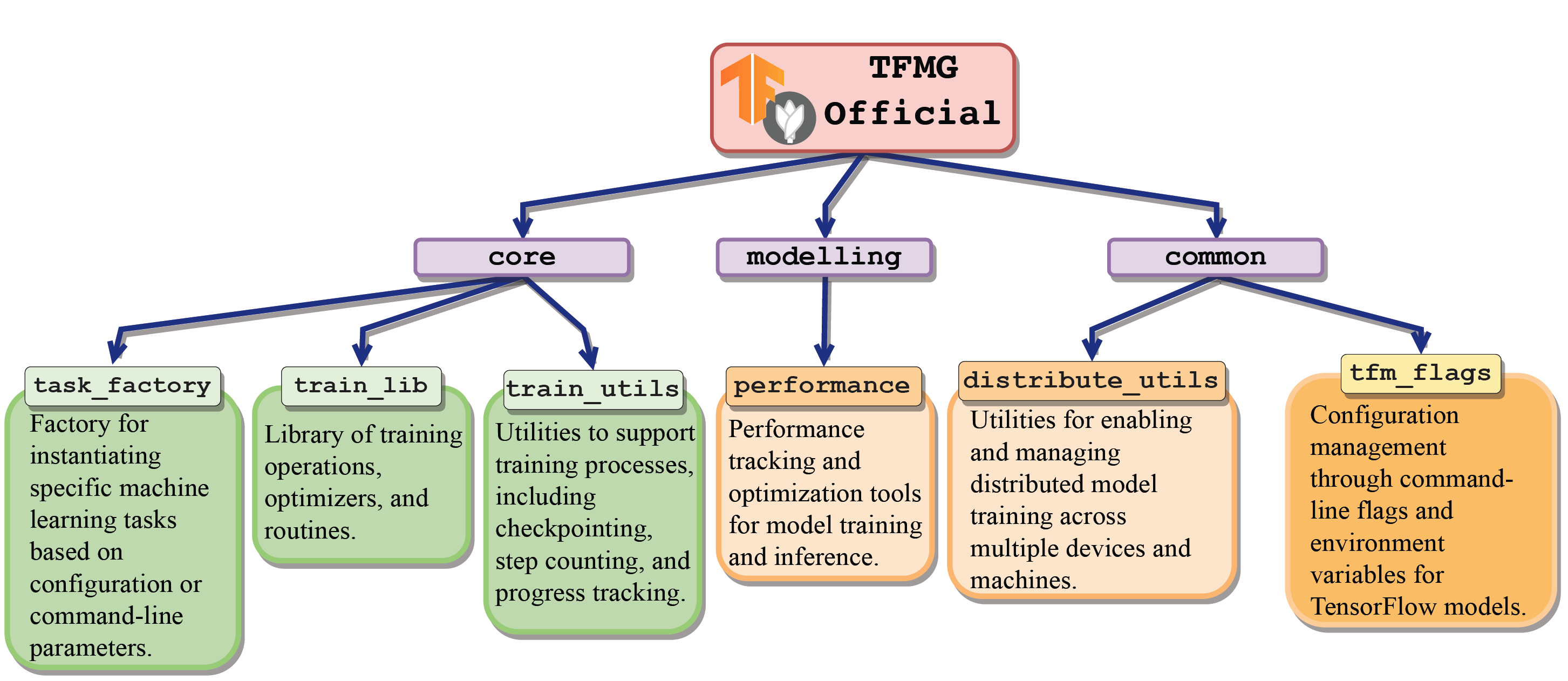
Figure 2: Overview of the TensorFlow Model Garden (TFMG) architecture. The diagram illustrates the modular design of the TFMG framework, highlighting the key components such as ‘task_factory’ for initializing machine learning tasks, ‘train_lib’ for training operations, ‘train_utils’ for training utilities, ‘core’ for central functionalities, ‘modeling’ for model definitions, ‘performance’ for tracking and optimization, ‘distribute_utils’ for distributed training support, and ‘tfm_flags’ for configuration management. Arrows indicate the direction of dependencies between modules.

The advent of universal architectures, as exemplified by DETR Carion et al. (2020), has revolutionized the field of image segmentation, demonstrating that mask classification architectures equipped with an end-to-end set prediction objective possess the versatility required for any segmentation task. Building on this foundation, MaskFormer further illustrates the efficacy of DETR-based mask classification, not only excelling in panoptic segmentation but also setting new benchmarks in semantic segmentation performance. This progression underscores a significant shift towards more generalized and efficient frameworks for tackling the diverse challenges of image segmentation. In this work, we reproduce the MaskFormer architecture in TensorFlow with inference and training supported on TPUs.

3 Overview of TensorFlow Model Garden Library

The TensorFlow Model Garden (TFMG) Yu et al. (2020) is a comprehensive suite of state-of-the-art machine learning models, particularly focused on vision and natural language processing (NLP). It offers both official models maintained by Google engineers and research models from academic papers, along with tools for easy configuration and deployment on standard datasets.

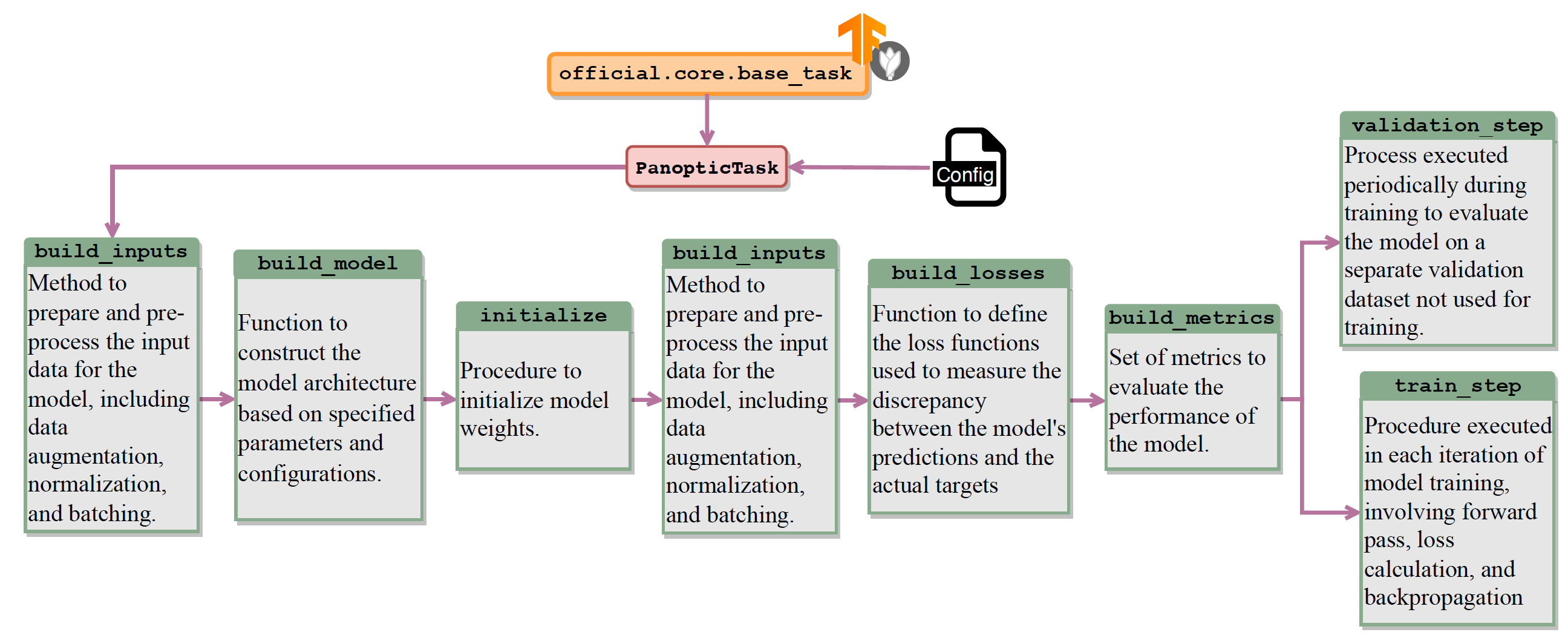
Figure 3: Illustration the workflow components of a machine learning task, centralized around ‘PanopticTask’. It includes the configuration, model building, initialization, and input preparation stages, followed by training and validation steps. ‘build_losses’ and ‘build_metrics’ are essential for calculating model performance during training.

In this section, we highlight key TFMG components instrumental in developing the MaskFormer model in TensorFlow. The Table 1 provides an organized summary of the submodules in TFMG. These components range from well-maintained official models to cutting-edge research models and include a streamlined training environment as well as specialized operations tailored for vision and NLP tasks. This modular overview encapsulates the diverse utilities offered by TFMG for model development. The MaskFormer model’s development harnesses the official module of TFMG, which encompasses a suite of submodules crafted for general model development. These submodules provide a foundation for tasks such as initializing specific machine learning tasks, managing training operations, optimizing model performance, and configuring distributed model training across multiple devices. A detailed visualization of the submodules, along with their specified functionalities within the TFMG official module is shown in Figure 2.

Typically, the development of a model utilizing the TFMG follows a structured sequence of steps. Following is the sequence of steps which are described in detail in subsequent sections:

1. Project Structure Organization: Every project developed using TFMG requires following a well-defined structure to ensure the seamless integration of various components and to facilitate efficient development workflows. Specifically for MaskFormer, we follow the following directory structure. for tree= font=, grow’=0, child anchor=west, parent anchor=south, anchor=west, calign=first, inner xsep=7pt, edge path= [draw, edge] (!u.south west) +(7.5pt,0) |- (.child anchor) pic folder edge label; , before typesetting nodes= if n=1 insert before=[,phantom] , fit=band, before computing xy=l=15pt, [TFMG official [projects - A high-level project directory for all the TFMG projects [maskformer - MaskFormer project directory. [configs - Contains model parameters and training settings.] [data - Contains scripts for creation of TFRecords.] [dataloaders - Contains data reader and parser for dataloader.] [losses - Contains implementation of loss functions] [modeling - Architecture implementation.] [tasks - Contains MaskFormer task that coordinates training and testing.] [utils - Contains utility functions.] ] […] ] ]

2. Compute and Environment: We set up the training environment using Google Cloud Platform (GCP) which offers scalable and versatile computing resources. Our implementation of MaskFormer has been designed to support training on both GPU (Graphics Processing Unit) and TPU (Tensor Processing Unit) platforms with the help of official.common.distribute_utils. The configuration of the distributed training is all handled by the training driver script described in step 5.

3. Task Specification: The modular architecture of TFMG is designed for the seamless addition of new models through precise task specification, which is typically encapsulated in a script named <task_name>.py, located within the tasks directory. At a higher level, these task specifications play a critical role in the model training process. They are utilized by the training driver script to initialize various critical aspects of model training, including setting up the training and validation processes and defining the metrics to evaluate model performance. In the specific case of the MaskFormer model, customization within our framework is achieved by extending the base_task class, which is sourced from official.core. By overriding several of its member functions, we tailor the underlying implementation to meet the unique requirements of the MaskFormer model. An illustration of the modified member functions of the base class for MaskFormer with their corresponding functionalities is shown in Figure 3. The implementation details of these functions are delineated in subsequent sections.

4. Configuration Specification: This step involves detailing the parameters related to training and model configuration, including the hyperparameters critical for model performance optimization. This process is facilitated through the extension of the official.core.config_definitions.TaskConfig class, which acts as a container for all requisite model parameters. The organization of configuration parameters is arranged, adhering to their functional relevance. This is achieved by grouping them under distinct classes derived from official.modeling.hyperparams. Some of the systematically defined hyperparameter classes for MaskFormer include:

   • Parser: Specifies the parameters for preprocessing input data, including output size, scale, and aspect ratio range.

   • DataConfig: Outlines the settings for input data handling, such as paths to training and validation datasets, batch sizes, and data augmentation strategies.

   • MaskFormer: Details the structural specifics of the MaskFormer model, including the number of queries, hidden size, and the backbone used.

   • Losses: Enumerates the different losses used during training, including class offset, background class weight, and L2 weight decay.

   • PanopticQuality: A custom evaluator configured to assess the panoptic quality (PQ) of our model’s predictions

   Note that these configs can be overridden by the user via the command line or by passing a yaml file to the training command.

5. Training Driver Script: (train.py) The script serves as a training driver for the project. It handles the setup and execution of model training and evaluation across different computing environments, including CPU, GPU, and TPU. Key steps include parsing configuration specified in step 4, setting up the appropriate TensorFlow distribution strategy based on the computing environment (step 2), initializing the model and task based on provided configurations (step 4), and running the training or evaluation process (step 3). The TFMG project uses Orbit Trainer as a lightweight and flexible training and evaluation loop. Orbit simplifies the creation of custom training loops, reducing the boilerplate code. It supports both eager execution and graph execution modes.

4 Architecting MaskFormer in TensorFlow for TPUs

In this section, we provide a concise overview of the data-loader, architecture, and loss functions that are key components critical to the reproducibility of MaskFormer.

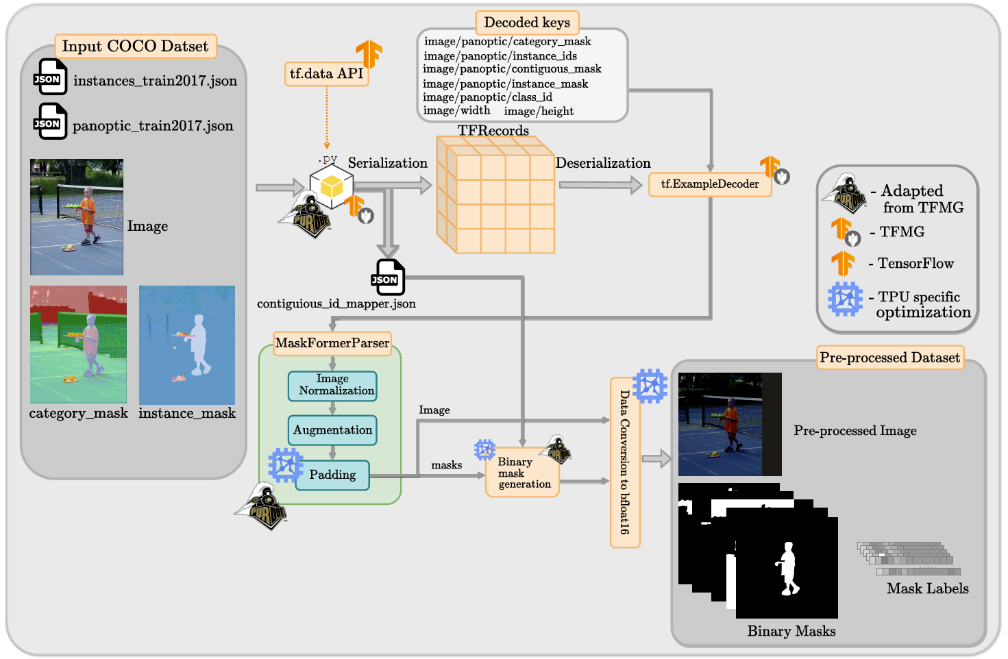
Figure 4: Illustration of the data pre-processing pipeline for panoptic segmentation task, specifically for training MaskFormer model with ‘COCO’ dataset. The process begins with the raw image and annotation files (JSON format), which are serialized into TFRecord format, a TensorFlow-specific binary storage format. Subsequently, these TFRecords are deserialized, and the data is passed through a series of preprocessing steps including normalization, augmentation, and padding to ensure uniformity of the input data. The binary mask generation and the label mapping are integral to preparing segmentation tasks. The output is then converted to a format compatible with the model’s data loader, which feeds the processed data into the training pipeline. (zoom in for a better viewing experience)

4.1 Dataset & Data loader

4.1.1 Dataset

In the context of our reproducibility project focused on the MaskFormer architecture, we chose to employ the COCO (Common Objects in Context) Lin et al. (2014) dataset as the primary benchmark for training and evaluation. As a first step towards data preparation, we need to create the TFRecords, which is a binary file format used by TensorFlow for storing data. It supports the inclusion of various types of annotations such as detection bounding boxes, instance segmentation masks (optionally encoded as PNG images), and textual captions. For the creation of TFRecords of the COCO dataset, a standardized script is made available from the TFMG Vision package. Specifically, we adapt the base implementation create_coco_tf_record.py made available at official > vision > data.

The MaskFormer architecture differs from existing panoptic segmentation models available on the TFMG by its unique requirement for per-object binary masks which have their corresponding class labels for loss calculation. In order to facilitate this we propose following to existing base implementation of create_coco_tf_record.py as follows:

• Conversion of non-contiguous coco class ids into contiguous : By default in the COCO dataset, class IDs are non-contiguous, meaning there are gaps in the sequence of IDs used to label object categories. For our implementation, we adopted an approach to manage the conversion between non-contiguous (original) class IDs from the COCO dataset and contiguous IDs. We maintain a mapping between non-contiguous (original class ids) and the contiguous ids facilitated by a mapping stored in contiguous_id_mapper.json. This JSON mapping file acts as a lookup table, where each original class ID from the COCO dataset is associated with a new, contiguous ID. By utilizing this mapping, we can easily convert the non-contiguous class IDs present in the ‘category_masks’ for the COCO dataset to a ‘contiguous_mask’. Further, the ‘contiguous_mask’ is used by the binary mask generation step in the dataloder (described in the next section). An illustration of TFRecord creation is shown in Figure 4.

The final output of the TFRecord creation step is a set of binary files also known as shards. Each shard contains a subset of the dataset, formatted as TFRecord entries that TensorFlow can efficiently load. In TensorFlow’s TFRecord format, data is serialized into a string format and stored in a key-value pair within a tf.train.Example message. The keys in this context are used to specify the type of data stored, allowing each data element to be uniquely identified and correctly deserialized during the data loading process. The set of keys used by our implementation is shown in Figure 4.

4.1.2 Dataloader

The data pipeline for training MaskFormer consists of several stages. Our work reuses some of the stages of the data pipeline directly from pre-existing TFMG modules and customizes only the input reader and parser. The stages of the data pipeline are briefly described below along with our proposed modifications.

Input Decoder and Parser: The input decoder serves as the primary interface with the dataset, responsible for fetching the raw data. We integrate and adopt the input_reader.py from official > vision > dataloaders directory of TFMG.

Decoder: We customize the base TFExampleDecoder class from official.vison.dataloaders.tf_example_decoder. This customization involves augmenting the class’s initialization process to incorporate additional keys that are specific to the TFRecords generated for our TFRecords as explained in Section 4.1.1. By introducing these new keys during the class’s instantiation, we ensure that our decoder is equipped to recognize and appropriately process these specialized data fields. The new keys are used by the decode member function.

Parser: Once the data is decoded from the decoder the parser handles all the pre-processing operations. We inherit the parent parser from official.vision.dataloaders and override required member functions. Firstly the role of the parser can be abstracted into two functional parts:

• Image and Mask Processing : Normalizes images, resize images, and masks to target dimensions and potentially applies data augmentation techniques like random horizontal flipping or cropping based on the training configuration. Notably, the implementation of random cropping is executed with a certain probability $p$ and the cropped images’ shortest side is resized to one of the predetermined sizes in the set [400px, 500px, 600px]. Further, we pad the cropped image and mask with zeros. Note that we explicitly ensure the padded region is ignored during the mask loss calculation step.

• Label Preparation : The primary aim of the Label Preparation step is to process the “contiguous_mask" annotations and generate individual masks for each object instance. These masks are then associated with their corresponding class IDs. The end-to-end process of data preparation is shown in Figure 4.

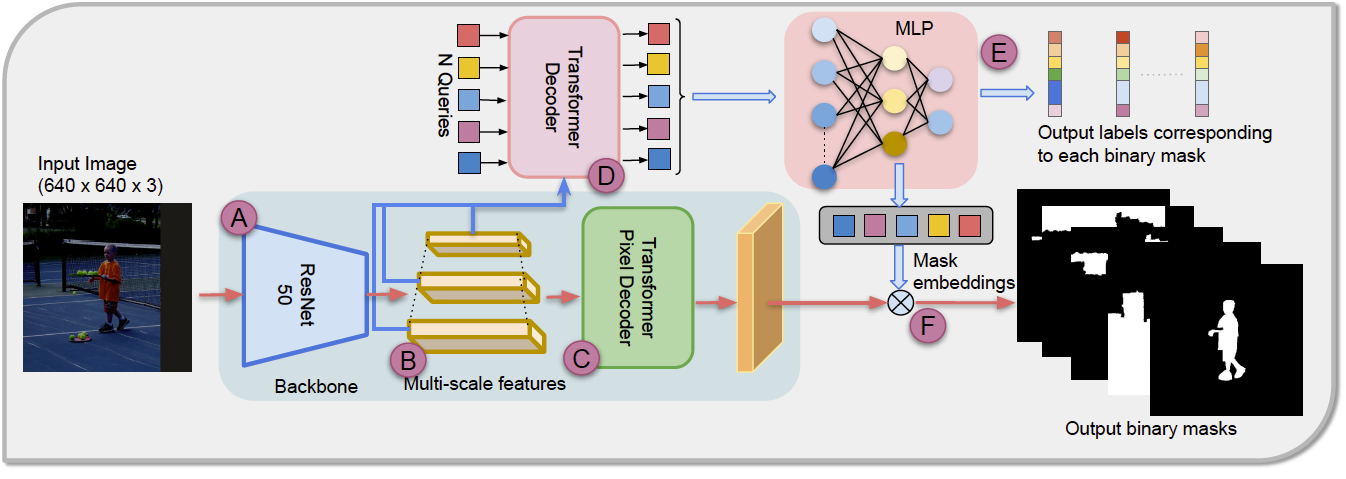
Figure 5: Illustration of MaskFormer architecture (reproduced from  Cheng et al. (2021).). The process begins with an input image (A), which is processed by a ResNet-50 backbone to extract feature maps. Multi-scale features (B) are generated from the backbone and then decoded by a Pixel Decoder (C) to create refined feature maps. These are fed into a Transformer Decoder (D), along with a set of learned queries that interact with the feature maps to generate mask embeddings (F). An MLP head (E) processes the mask embedding to produce the final segmentation output, which consists of binary masks for each query, along with their corresponding output labels, indicating the presence of specific objects or regions within the input image.

Figure 6: Detailed implementation overview of decoding stage of MaskFormer model. The architecture begins with the backbone features extracted from the input image. These features are then projected and enriched with positional embeddings before being passed through multiple layers of a Transformer encoder. The resulting encoded features are processed by a Transformer Pixel Decoder, which combines them with mask features to enhance localization capability. Simultaneously, query embeddings are combined with positional embeddings and processed by the Transformer Decoder to generate predictions. The decoded features are then passed through an MLP head, which classifies each pixel, resulting in the final output comprising predicted binary masks and their associated labels.

4.2 Model Architecture Implementation Overview

An overview of the MaskFormer architecture is illustrated in Figure 5. Key components and functionalities of the MaskFormer architecture are outlined as follows:

• Backbone Network : The original work explored a diverse array of backbone networks for feature extraction, encompassing both convolutional architectures, such as ResNet-50 He et al. (2016), and transformer-based models like the Swin Transformer Liu et al. (2021). The ResNet50 implementation is readily available in TFMG under official > vision > modeling > backbones and the pre-trained checkpoint for ResNet are made available at TF-Vision Model Garden found under official > vision.

• Multiscale Features : In our model’s architecture, a key component is the utilization of multiscale features, as indicated by the ‘B’ in Figure 5. This design choice allows for flexibility in feature extraction from the backbone network, specifically ResNet. Our implementation supports both the extraction of deep, high-level features from the final layer of ResNet and the rich, intermediate features available from earlier layers. An important consideration when employing the multiscale features is the increased demand for memory during the model training phase. The inclusion of data from multiple layers escalates the volume of information processed, which can strain available memory resources. In our implementation, the use of multi-scale features is controlled by the parameter deep_supervision.

• Transformer Pixel Decoder : A comprehensive depiction of the transformer pixel decoder’s architecture is illustrated in Figure 6. At its core, the transformer pixel decoder is an assembly of two primary components: the transformer encoder and a series of convolutional and normalization layers. We have incorporated the transformer encoder layers into our architecture by utilizing the existing implementation available in the TensorFlow Model Garden, specifically from the directory official > nlp > layers. To maintain consistency and interoperability with models developed in other frameworks, particularly PyTorch, we have undertaken a process to ensure that our adopted transformer encoder layers exhibit functional parity with their PyTorch counterparts. This involves a series of rigorous verification steps, designed to thoroughly compare and validate the behavior and the output shapes of the encoder layers. The detailed steps we followed for verification are described in section 5. The remaining set of convolution and normalization layers in our architecture are implemented utilizing the TensorFlow API.

• Transformer Decoder : Similar to our approach with the Pixel Decoder, we have adopted the Transformer Decoder component from the pre-existing implementations provided in the TensorFlow Model Garden, specifically sourced from the directory official > nlp > layers. While integrating the Transformer Decoder from the TensorFlow Model Garden, we ensure that it seamlessly interfaces with other components of our model, such as the transformer pixel decoder and the backbone network. This involves aligning input and output dimensions, ensuring compatible data types, and configuring the decoder appropriately to match our specific requirements. We validate and test the functionality of the integrated transformer decoder and the transformer pixel decoder within our architecture.

• MLP Projection : The MLP (Multi-Layer Perceptron) projection layers, in conjunction with the linear classifier, are used to obtain the predicted binary masks and corresponding labels. The Transformer Decoder processes the Transformer Encoder Features to extract high-dimensional features, Transformer Features, that encapsulate both spatial and contextual information are used by the linear classifier to predict the label of each binary mask. Simultaneously, Mask Features that are obtained from the Transformer Pixel Decoder are fed into the MLP projection layers to obtain the predicted binary masks. We implement the Head of MaskFormer using TensorFlow API.

4.3 Loss Functions

In this section, we provide in-depth implementation details of various components for the loss calculation process. The function module consists of a matcher and mask losses (focal, dice, and classification loss). The loss calculation first starts with the step of matching between the predicted outputs and the ground truth as there is no guarantee about the prediction order of the masks and labels followed by calculating all the losses. A detailed description is provided below :

• Matcher : Given a set of $N$ ground truth binary masks for objects in an image, denoted by $\{\mathbf{M}_{\text{GT}}^{i},\mathbf{Y}_{\text{GT}}^{i}\}_{i=0}^{N}$, where $\mathbf{M}^{i}_{\text{GT}}$ and $\mathbf{Y}_{\text{GT}}^{i}$ represent the $i^{\text{th}}$ ground truth binary mask and label, respectively. Let the predicted set of binary masks and class labels be denoted by $\{\mathbf{M}_{\text{pred}}^{i},\mathbf{Y}_{\text{pred}}^{i}\}_{i=0}^{\text{n\_queries}}$, where $\text{n\_queries}=100$ is the fixed number of predictions made by the model. Given the variable number of ground truth masks per image and the fixed number of predicted masks and labels, it is necessary to find the correct order of masks so that the loss calculation for a given ground truth mask is not performed with any arbitrary predicted mask. In the original PyTorch implementation, the matching step was facilitated by the scipy.optimize.linear_sum_assignment function, which provided the correct ordering of masks. This function requires a cost matrix as input, which is used to determine the cost of matching a given ground truth with a prediction. When $N<\text{n\_queries}$, the cost matrix is rectangular. The cost calculation involves evaluating the focal, dice, and classification losses (to be explained in a subsequent section) and weighting them with predetermined weights. The order of the predictions is disregarded at this step. However, directly applying the scipy.optimize.linear_sum_assignment function on tensors can significantly reduce training performance on TPUs.

• Dice Loss: Dice Loss is employed to supervise the prediction of masks, offering a measure of similarity between the predicted binary masks and the ground truth masks. It is particularly effective for handling imbalanced datasets where the presence of the class of interest significantly varies across samples. The formulation of Dice Loss is based on the Dice coefficient (also known as the Sørensen-Dice coefficient), which calculates the overlap between two samples. Mathematically, it is defined as:

  $$\text{Dice Loss}=1-\frac{2\times|\mathbf{Y}_{\text{pred}}\cap\mathbf{Y}_{\text{GT}}|}{|\mathbf{Y}_{\text{pred}}|+|\mathbf{Y}_{\text{GT}}|}$$

  where $\mathbf{Y}_{\text{pred}}$ represents the predicted mask and $\mathbf{Y}_{\text{GT}}$ represents the ground truth mask. This loss function encourages the model to increase the overlap between the predicted and true masks, thereby improving the accuracy of the predictions for the presence of objects within an image. We implement the dice loss using TF API and ensure that extra padded regions are ignored for calculating the loss.

• Focal Loss: Focal Loss is designed to address class imbalance by modifying the standard Cross-Entropy Loss in such a way that it places more focus on hard, misclassified examples. This is achieved by adding a modulating factor to the Cross-Entropy formula, which decreases the loss for well-classified examples, pushing the model to prioritize the learning of difficult cases. Focal Loss is particularly useful in scenarios where there’s a significant imbalance between the foreground and background classes, as often encountered in object detection tasks. The formula for Focal Loss is given by:

  $$\text{Focal Loss}=-\alpha_{t}(1-p_{t})^{\gamma}\log(p_{t})$$

  where $p_{t}$ is the model’s estimated probability for the class with label $t$, $\alpha_{t}$ is a weighting factor for the class $t$, and $\gamma$ is the focusing parameter that adjusts the rate at which easy examples are down-weighted. We implement the focal loss using TF API and ensure that extra padded regions are ignored for calculating the loss.

• Classification Loss: Classification Loss measures the discrepancy between the predicted class probabilities and the actual class labels of the training examples. We implement the cross entropy loss using TF API and ensure that labels with no objects padded labels are downweighed with a pre-defined weight for calculating the loss.

4.4 Training and Hyper-Parameter Tuning

In this section, we delve into the convergence challenges that emerged during the model training process, as well as the hyper-parameter tuning that was essential for overcoming these obstacles. The default parameters inherited from the original implementation proved to be inadequate for facilitating training convergence. Some of the critical hyper-parameters that were tuned are enumerated below.

Weight Initialization : The standard layer implementations within TFMG diverge from the original MaskFormer implementation, particularly in terms of weight initialization. Such discrepancies can significantly impact model performance and convergence. In our implementation, we ensured that the weight initialization of all the layers matched the original implementation and observed that the weight initialization for the Head played a critical role.

Batch Size : The batch size hyper-parameter turned out to be one of the critical parameters that needed to be tuned to obtain smooth training convergence. Utilizing a smaller batch size for debugging purposes inadvertently led to a model that overfitted the background class.

No object class weight : The primary purpose of this hyper-parameter is to balance the model’s attention between areas with objects and areas without objects. In many images, the vast majority of the image might not contain any objects of interest. Without proper weighting, the model could become biased towards predicting no object most of the time, because it might minimize the loss more effectively by doing so. This would be counterproductive to the goal of detecting the often much smaller areas that do contain objects. Hence, this parameter needs to be tuned specifically for each dataset. In the original implementation, a no-object weight of 0.1 was used. However, in our version, employing a weight of 0.1 led the model to overfit towards predicting the absence of objects exclusively, always classifying regions as devoid of objects.

In addition to the previously mentioned hyper-parameters, there are numerous other settings, such as gradient clipping and warm-up phases, that can be adjusted to potentially enhance model performance further. Nonetheless, our experience indicated that the three highlighted hyper-parameters were the most crucial for ensuring the model’s generalization capabilities. Due to the constraints of this reproducibility project and compute, we were unable to conduct a more in-depth exploration of the hyper-parameters.

5 Verification

Previous research has highlighted effective strategies for reengineering deep learning models, as noted in works by Jiang et al. (2023a); Banna et al. (2021). We adopted these practices for our replication process. In this section, we will provide a detailed, step-by-step account of the procedures we adhered to during our reimplementation efforts.

5.1 Shape Testing

Shape testing plays a crucial role in verifying that the data flowing through the model’s layers conforms to expected dimensions. Specifically, in models like MaskFormer where multiple modules are interacting with each other, the tensor shapes must be compatible across modules. Given below are the systematic steps we used to verify the shapes of the tensors.

• Input Shape Validation: We started by validating the shape of the input data. We ensured that at various stages, from converting the raw dataset to TFRecords to processing in the dataloader before and after padding, the final output of the dataloader matched the input shape required by the MaskFormer model. This step helped identify any preprocessing errors or mismatches in data augmentation procedures.

• Layer-wise Output Shape Verification: For each layer in the model, we programmatically checked the output shapes by feeding a randomly initialized tensor. This verification process is essential to confirm that the transformations applied by each layer (such as convolutions, pooling, transformer layers, and fully connected layers) yield outputs of the correct dimensions. It also helps in identifying layers where shape mismatches occur, facilitating quicker debugging.

• Final Output Shape Check: The last step in shape testing involved validating the shape of the model’s final output against the expected dimensions. This ensures that the model’s predictions or classifications can be correctly interpreted and applied to downstream tasks.

5.2 Unit Testing

Unit testing involves testing individual sub-components or components of the MaskFormer to ensure that the implementation is bug-free and functionally equivalent to the PyTorch code.

• Functionality Tests for Customized Modules : While customizing the existing code from TFMG, we incorporated several custom layers and functions. To ensure their independent and correct functionality within the model, we devised a comprehensive suite of unit tests. These tests not only encompass the previously described shape tests, which verify the dimensions of data flowing through the model but also rigorously evaluate the actual outputs against expected results for predefined inputs. For instance, in the case of custom loss functions, our validation process involved feeding the model with carefully selected tensors that have known loss values derived from the original model’s computations. We then compared the loss values output by our customized implementation against these benchmarks. To quantify the precision of our custom loss function, we established an acceptance threshold: the computed loss values should exhibit negligible deviation from the expected ones, with differences constrained to within $\leq 0.001$.

• Gradient Flow and Magnitude Checks : Ensuring that gradients correctly flow through the model’s layers is vital for the training process. We employed unit tests to check gradient computation and propagation, particularly in custom components where automatic differentiation might face complexities.

• Model Component Integration Testing: Beyond testing individual layers or functions, we also conducted tests on how these components integrate. For instance, testing the integration of newly introduced layers with existing ones or verifying the compatibility of custom loss functions with the model’s output.

• Error Handling and Edge Cases: Finally, we wrote unit tests to cover error handling and edge cases. This includes testing the model’s behavior when provided with invalid input types, sizes, or values and ensuring that the model fails gracefully or throws meaningful errors.

Table 2: Comparison of module shapes and mean outputs between original PyTorch and our TensorFlow implementations. ($\dagger$) The table particularly highlights the differences in the output values of the Transformer Decoder module (first row in table). There, the mean output in TensorFlow is notably different due to the inclusion of an additional convolutional layer that is not present in the PyTorch implementation. We use randomly initialized tensors with appropriate shape for shape testing.

Module	Torch Shape	TF Shape	Mean Output (Torch)	Mean Output (TF)
Transformer Decoder $\dagger$	[1, 100, 256]	[1, 100, 256]	-0.0026	-1.5832484e-09
Transformer Pixel Decoder	[1, 256, 160, 160]	[1, 160, 160, 256]	0.0542	0.011979061
PosEmbed	[1, 256, 20, 20]	[1, 20, 20, 256]	0.4937	0.49366885
MLPHead	N/A	N/A	[0.012966,1.593415]	[0.012966, 1.593414]
Classification loss	N/A	N/A	0.06040	0.06043
Focal loss	N/A	N/A	0.2129	0.21077
Dice loss	N/A	N/A	0.2980	0.29806

5.3 Differential Testing

Weight loading

To conduct differential testing on our architecture, it is imperative to first import the pre-trained weights. However, unlike previous replication efforts Banna et al. (2021), we encountered a significant obstacle: the absence of an open-source TensorFlow checkpoint for MaskFormer. The absence of directly compatible pre-trained weights complicates differential testing on the model, necessitating manual framework-to-framework conversion. This process is time-consuming and requires meticulous verification to ensure (1) successful transfer of weights for each layer, and (2) correctness of all converted weights.

In an initial attempt to bridge this gap, we explored the possibility of converting MaskFormer’s pre-trained weights, hosted on its GitHub repository, into the Open Neural Network Exchange (ONNX) format ONN (2019). ONNX is designed as an open format to represent machine learning models and facilitates interoperability between different frameworks, including PyTorch and TensorFlow Jajal et al. (2023). Theoretically, this approach should have allowed us to leverage open-source model converters, such as torch2onnx and onnx-tf, to transition the model’s checkpoints from the Torch format to TensorFlow. The conversion process involves loading the .onnx model and converting it into a .pb TensorFlow graph, which is subsequently loaded into tensorflow. This process generally preserves the structure of the model but does not facilitate direct manipulation or extraction of weights as individual tensor objects. Instead, the converted static graph, running on the tf-backend, encapsulates both the architecture and the weights but prevents the transfer of individual layer weights to an existing TensorFlow model as a separate entity.

To surmount these challenges, we developed a custom converter tool capable of directly translating the weights from PyTorch to TensorFlow. This manual conversion process involved intricate mapping and adaptation of model parameters, ensuring compatibility and functional integrity of the architecture in its new framework. Our tool not only addresses the immediate issue of importing pre-trained weights but also contributes to the broader field by offering a potential workaround for similar conversion challenges involving complex models with framework-specific operations. A summary of the differential testing output comparison between our implementation and the original PyTorch implementation is shown in Table 2. Our custom converter tool is available at this link.

6 Debugging and Performance Evaluation

In this section, we outline the debugging setup used for the development of MaskFormer, as well as a qualitative assessment of the trained model. Owing to computational constraints, our evaluation is preliminary but presents substantial proof of the efficacy of our implementation. It indicates that with extended training time and hyper-parameter optimization, our implementation has the potential for significant improvements.

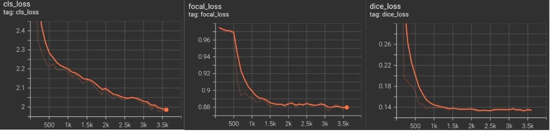
Figure 7: Loss Curves Visualization on TPUs using TensorBoard: raw loss values (light color) and smoothed values (dark color).

6.1 Debugging Setup and Tools

The setups we used for debugging and training our model are as below:

• Debugging: Our debugging setup to dry run and test various components of MaskFormer consisted of an AMD EPYC 7543 32-core Processor and a single NVIDIA A100 (80GB) GPU. We utilized TensorFlow’s eager execution mode for line-by-line debugging. Additionally, we employed logging via TensorBoard for real-time monitoring of the loss function, gradients, and activations. Additionally, one can also debug the model using CPU, however, it would be very slow and will require a significant amount of RAM. The dry runs on GPU are limited to the input image size of 640 x 640 with a batch size of 1.

• Training : Our model training infrastructure uses Cloud TPUs provided by Google Cloud Platform (GCP). Specifically, we use TPU node architecture. The architecture of the TPU Node is designed such that the user VM interacts with the TPU host using gRPC for communication. In this setup, direct access to the TPU Host is not possible, which can complicate the process of debugging training sessions and resolving TPU-related issues. However, several visualization tools are made available by GCP to monitor various aspects of the training and debugging process. Some useful monitoring tools that we found useful include as detailed below.

  The Google Cloud Platform (GCP) offers a comprehensive suite of monitoring tools designed to track the performance and health of Cloud TPUs. Using Google Cloud Monitoring, you can automatically collect metrics and logs from both the Cloud TPU and its associated Compute Engine host.

  

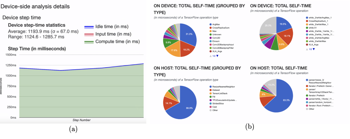
  Figure 8: TPU Profiling Results. Subfigure (a) displays the device step time breakdown, while subfigure (b) illustrates the time allocation for different operations on the device and the host. Using the time spent on operations shown in subfigure (b) one can identify specific costly operation like ArgMax operation on TPU and optimize our implementation.

  Key Monitoring Tools and Features in GCP

  • Metrics Collection: Automatic tracking of numerical quantities over time, such as CPU utilization, network traffic, and Tensor Cores’ idle durations. These metrics are crucial for gauging the performance and resource consumption of Cloud TPUs.

  • Logging Capabilities: Logs are essential for documenting events at precise moments. Generated by Google Cloud services, third-party applications, or custom code, these log entries are instrumental in troubleshooting. Creating log-based metrics from these entries allows for transforming log data into actionable insights.

  • Viewing and Querying Data: The Metrics Explorer in Cloud Monitoring allows for the real-time visualization of metrics. Advanced queries can be made using HTTP calls or the Monitoring Query Language for in-depth data analysis.

  • Prerequisites and Setup: Initial requirements include a Compute Engine VM and Cloud TPU resources, alongside a basic understanding of Google Cloud Monitoring.

  • Detailed Metrics for TPUs: Specific metrics provided for TPUs include memory/usage for monitoring memory usage, network/received_bytes_count and network/sent_bytes_count for network traffic, cpu/utilization for CPU load, and tpu/tensorcore/idle_duration for tracking Tensor Cores’ activity.

  TPU Profiling

  Profiling the model on Cloud TPU Nodes with TensorBoard and the Cloud TPU TensorBoard plugin is critical for optimizing training performance. This involves capturing profiles either via the TensorBoard UI or programmatically, which then allows for a deep dive into performance metrics.

  • TPU Utilization: Measures how effectively the TPU resources are being used.

  • CPU Utilization: Indicates the processing load on the CPU.

  • Memory Usage: Tracks the memory consumption of both the TPU and the host machine.

  • Infeed/Outfeed Rates: Analyze the data transfer rates to and from the TPU, identifying potential bottlenecks.

  • TensorFlow Operations Time: Highlights the most time-consuming TensorFlow operations.

  • Step Time: Average duration of each training step, providing insights into overall model efficiency.

  For further guidance on capturing and analyzing these metrics, consult Google Cloud’s documentation on TPU profiling tools.

• Data Storage : We store the TFRecords in a GCP bucket, located in the same zone as our TPU nodes to enhance data access speed and efficiency. This setup minimizes latency and maximizes throughput.

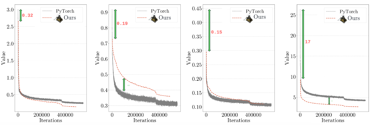
Figure 9: Comparative convergence plots of loss values over training iterations for models implemented in PyTorch and TensorFlow. From left to right: Classification Loss, Dice Loss, Focal Loss, and Total Loss.

6.2 Qualitative Results

We organize the qualitative evaluation of our model into two distinct sections:

6.3 Training Performance Analysis

This section delves into the performance of the model during the training phase. We assess how well the model learns and adapts to the training dataset, which is crucial for its ability to generalize from the training examples provided. Utilizing the TPU profiling and monitoring tools, we examine a variety of metrics, such as CPU and TPU utilization, memory usage, and data transfer rates, as detailed in section 6.1. This analysis helps us identify potential bottlenecks in our training process and informs decisions on model adjustments and optimizations to enhance learning efficacy.

TPU Profiling Results : During the development of MaskFormer, we periodically leveraged the TPU profiling tool to assess bottlenecks in the training pipeline. The TPU profiling results, as depicted in Figure 8, provided us with invaluable insights into the efficiency of our model’s computations. Figure 8(a) illustrates the device step time, which includes the average, range, and standard deviation of time taken for each step in milliseconds. The step time is further broken down into idle time and compute time, indicating periods when the TPU is not actively processing. This granularity allowed us to identify and minimize idle times by optimizing the input pipeline and ensuring a consistent feed of data into the TPU, thus reducing the time spent waiting for data.

Figure 8(b) presents a comprehensive breakdown of the self-time spent on different types of operations both on the device and the host. The pie charts demonstrate the proportion of time consumed by various TensorFlow operations. For instance, on-device, we observed that a significant portion of time was devoted to matrix multiplication operations, which are computationally intensive but crucial for deep learning tasks. Meanwhile, the host spent a considerable amount of time on data preprocessing tasks. By analyzing these segments, we were able to fine-tune our model’s architecture and the data preprocessing steps to better balance the workload between the host and the TPU.

The profiling information guided us in optimizing our training loop. Adjustments made from these insights included tweaking batch sizes, streamlining TensorFlow operations to reduce complexity, and revising the scheduling of operations to avoid underutilization of the TPU.

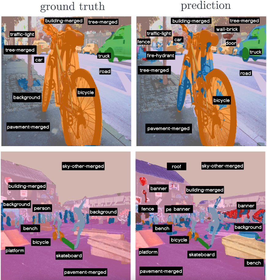
Figure 10: Side-by-Side Comparison of Ground Truth and Model Predictions.

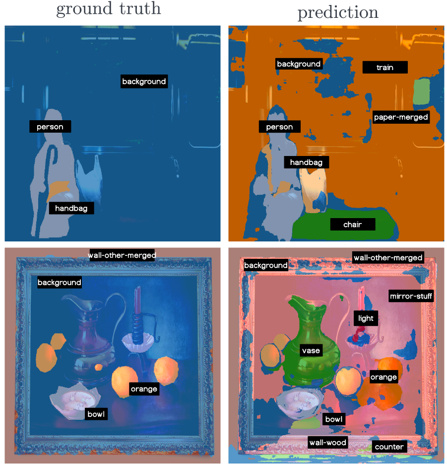
Figure 11: Side-by-Side Comparison of Ground Truth and Model Predictions.

6.4 Evaluation on the Test Set

Due to the limited scope of the project and constraints in computational resources, this section focuses exclusively on qualitative results obtained from the test set images. We provide a detailed visual examination of the model’s output, comparing it against ground truth.

Our evaluation begins with an examination of parameter count and FLOPs presented in Table 3 and a dry run of training with the loss curves visualized on TensorBoard, as presented in Figure 7. The figure shows the trajectories of three key loss components during training: classification loss, focal loss, and dice loss. Notably, all three loss components exhibit a downward trend, indicating successful learning. Furthermore, Figure 9 offers a comparative analysis of convergence plots, contrasting our model’s loss values over training iterations against the original model implemented in PyTorch. The plots illustrate the classification, dice, and focal losses, as well as the total loss. These graphs are particularly insightful as they show our model, denoted by the red dashed line, consistently achieving lower loss values earlier in the training process compared to the PyTorch implementation. This suggests that our model implemented in TensorFlow with TPU optimization converges.

Lastly, we assess the model’s performance through a direct visual comparison of predictions with ground truth, as illustrated in Figure 10 and 11. The side-by-side images display how the model segments various objects within urban street scenes. While the model demonstrates strong alignment with the ground truth in many cases, particularly in distinguishing between different categories of vehicles and urban infrastructure, there are discrepancies worth noting. For instance, the model occasionally misclassifies similar textures or confuses overlapping objects, challenges that are common in semantic segmentation tasks. These observations are instrumental in pinpointing areas where the model could be further refined to enhance its segmentation accuracy.

Table 3: Comparative Overview of DETR and MaskFormer Implementations. The table summarizes the differences in backbone structure, input size flexibility, and parameter count, between MaskFormer models implemented in PyTorch, and our MaskFormer implementation in TensorFlow.

Implementation	Backbone	Input size	# of parameters
MaskFormer-PyTorch	ResNet50 + 6 Encoder	Variable size	45.04M
MaskFormer-TensorFlow (ours)	ResNet50 + 6 Encoder	640 x 640	45.16M

7 Discussion

7.1 Project Cost

Table 4: Google Cloud Platform (GCP) Cost Report.

GCP Service	Details	Cost
Compute engine	Virtual machine instance	$4811.69
Cloud storage	Standard storage, data transfer	$796.89
Cloud logging	Log storage cost	$104.28
Networking	Network intelligence center resource hours	$23.33

We provide an estimate of the project’s cost in terms of both time and money for reference. Table 4 details the cost of Google Cloud Platform (GCP) resources. This cost omits the TPU time, to which Google gave us access for the project duration. During the one year of the project, we attempted two distinct organizations. Initially, two Ph.D. students led a team of ten undergraduate students for the first six months. For the remaining six months, the team composition changed to two Ph.D. students and one experienced undergraduate student.

7.2 Alternative approaches to ML model re-use (“Build vs. buy”)

Davis et al. described several paths to re-using machine learning models Davis et al. (2023). This study applied what they call conceptual re-use: given an existing paper and implementation, we developed an independent implementation targeting another development framework and hardware resources. This approach produces a model tailored to the hardware platform, with maximal adherence to the original paper Montes et al. (2022), and with no known backdoors or other security issues. However, the cost of a conceptual re-use approach is high (§7.1).

Pre-trained models (“adaptation re-use”) present an attractive pathway for model reuse that can significantly reduce the engineering overhead associated with custom optimizations Jiang et al. (2023c; b). The strength of PTMs lies in their versatility and the breadth of their training, which allows for a more straightforward adaptation to a variety of tasks without the need for extensive re-engineering Han et al. (2021). This characteristic of PTMs can accelerate the development cycle, and potentially can also help with the model reproducibility and replicability problem. Furthermore, with access to detailed training logs and configurations of open-source PTMs, there is potential for leveraging these resources to assess the accuracy of model replications across various frameworks, illustrating PTMs’ broader impact on fostering model consistency and reliability Jiang et al. (2023a).

The third path discussed by Davis et al. was deployment reuse. Interoperability tools, such as ONNX model converters, facilitate the adaptation of models across different frameworks and hardware Shen et al. (2021). Despite the potential for performance optimization on such hardware, deployment reuse also has hazards, e.g. model conversion errors Jajal et al. (2023); Openja et al. (2022).

These cost/benefit trade-offs underscore a key challenge in the reproducibility of AI research. Our findings emphasize the ongoing difficulties associated with training models on TPUs, primarily due to limited framework support and technical complications. We advocate for targeted research efforts to overcome these barriers, enhancing both the deployment efficiency and the replicability of models across diverse computational environments.

8 Conclusion

This paper documented our journey and methodologies in replicating the MaskFormer model from its original PyTorch implementation to TensorFlow, specifically optimized for TPUs. Given the limited compute resources and time constraints, our project achieved a partial replication, highlighting the significant engineering challenges and computational demands associated with such undertakings. Throughout this process, we encountered numerous technical hurdles, from framework-specific functionalities and model architecture discrepancies to weight conversion and optimization for TPU acceleration. To address these challenges, we developed custom tools, adapted existing TensorFlow functionalities, and proposed a detailed verification strategy to ensure the fidelity of our replication. Our systematic approach, detailed documentation, and the solutions we proposed aim to serve as a valuable resource for the community. By sharing our experiences and the lessons learned, we hope to contribute to the ongoing dialogue on enhancing reproducibility.

References

- ONN (2019) ONNX | Home, 2019. URL https://onnx.ai/.
- Badrinarayanan et al. (2015) Vijay Badrinarayanan, Alex Kendall, and Roberto Cipolla. Segnet: A deep convolutional encoder-decoder architecture for image segmentation. IEEE Transactions on Pattern Analysis and Machine Intelligence, 39:2481–2495, 2015.
- Banna et al. (2021) Vishnu Banna, Akhil Chinnakotla, Zhengxin Yan, Anirudh Vegesana, Naveen Vivek, Kruthi Krishnappa, Wenxin Jiang, Yung-Hsiang Lu, George K. Thiruvathukal, and James C. Davis. An Experience Report on Machine Learning Reproducibility: Guidance for Practitioners and TensorFlow Model Garden Contributors, 2021.
- Carion et al. (2020) Nicolas Carion, Francisco Massa, Gabriel Synnaeve, Nicolas Usunier, Alexander Kirillov, and Sergey Zagoruyko. End-to-end object detection with transformers. In European Conference on Computer Vision (ECCV), 2020.
- Chen et al. (2016) Liang-Chieh Chen, George Papandreou, Iasonas Kokkinos, Kevin P. Murphy, and Alan Loddon Yuille. DeepLab: Semantic image segmentation with deep convolutional nets, atrous convolution, and fully connected CRFs. IEEE Transactions on Pattern Analysis and Machine Intelligence, 40:834–848, 2016.
- Chen et al. (2018) Liang-Chieh Chen, Yukun Zhu, George Papandreou, Florian Schroff, and Hartwig Adam. Encoder-Decoder with atrous separable convolution for semantic image segmentation. In ECCV, pp. 833–851, 2018.
- Cheng et al. (2021) Bowen Cheng, Alexander G. Schwing, and Alexander Kirillov. Per-pixel classification is not all you need for semantic segmentation. In NeurIPS, 2021.
- Davis et al. (2023) James C Davis, Purvish Jajal, Wenxin Jiang, Taylor R Schorlemmer, Nicholas Synovic, and George K Thiruvathukal. Reusing deep learning models: Challenges and directions in software engineering. In 2023 IEEE John Vincent Atanasoff International Symposium on Modern Computing (JVA), pp. 17–30. IEEE, 2023.
- Han et al. (2021) Xu Han, Zhengyan Zhang, Ning Ding, Yuxian Gu, Xiao Liu, Yuqi Huo, Jiezhong Qiu, Yuan Yao, Ao Zhang, Liang Zhang, et al. Pre-trained models: Past, present and future. AI Open, 2:225–250, 2021.
- He et al. (2016) Kaiming He, Xiangyu Zhang, Shaoqing Ren, and Jian Sun. Deep residual learning for image recognition. In CVPR, pp. 770–778, 2016.
- Hutson (2018) Matthew Hutson. Artificial intelligence faces reproducibility crisis. American Association for the Advancement of Science, 359:725–726, 2018.
- Jajal et al. (2023) Purvish Jajal, Wenxin Jiang, Arav Tewari, Joseph Woo, George K Thiruvathukal, and James C Davis. Analysis of failures and risks in deep learning model converters: A case study in the onnx ecosystem. arXiv preprint arXiv:2303.17708, 2023.
- Jiang et al. (2023a) Wenxin Jiang, Vishnu Banna, Naveen Vivek, Abhinav Goel, Nicholas Synovic, George K Thiruvathukal, and James C Davis. Challenges and practices of deep learning model reengineering: A case study on computer vision. arXiv preprint arXiv:2303.07476, 2023a.
- Jiang et al. (2023b) Wenxin Jiang, Chingwo Cheung, George K Thiruvathukal, and James C Davis. Exploring naming conventions (and defects) of pre-trained deep learning models in hugging face and other model hubs. arXiv preprint arXiv:2310.01642, 2023b.
- Jiang et al. (2023c) Wenxin Jiang, Nicholas Synovic, Matt Hyatt, Taylor R Schorlemmer, Rohan Sethi, Yung-Hsiang Lu, George K Thiruvathukal, and James C Davis. An empirical study of pre-trained model reuse in the hugging face deep learning model registry. In 2023 IEEE/ACM 45th International Conference on Software Engineering (ICSE), pp. 2463–2475. IEEE, 2023c.
- Kirillov et al. (2018) Alexander Kirillov, Kaiming He, Ross B. Girshick, Carsten Rother, and Piotr Dollár. Panoptic segmentation. In CVPR, 2018.
- Kirillov et al. (2023) Alexander Kirillov, Eric Mintun, Nikhila Ravi, Hanzi Mao, Chloe Rolland, Laura Gustafson, Tete Xiao, Spencer Whitehead, Alexander C. Berg, Wan-Yen Lo, Piotr Dollár, and Ross Girshick. Segment anything. In ICCV, 2023.
- Lin et al. (2014) Tsung-Yi Lin, Michael Maire, Serge Belongie, James Hays, Pietro Perona, Deva Ramanan, Piotr Dollár, and C. Lawrence Zitnick. Microsoft COCO: common objects in context. In ECCV, 2014.
- Liu et al. (2021) Ze Liu, Yutong Lin, Yue Cao, Han Hu, Yixuan Wei, Zheng Zhang, Stephen Lin, and Bingshan Li. Swin transformer: Hierarchical vision transformer using shifted windows. In ICCV, pp. 10012–10022, 2021.
- Montes et al. (2022) Diego Montes, Pongpatapee Peerapatanapokin, Jeff Schultz, Chengjun Guo, Wenxin Jiang, and James C Davis. Discrepancies among pre-trained deep neural networks: a new threat to model zoo reliability. In Proceedings of the 30th ACM Joint European Software Engineering Conference and Symposium on the Foundations of Software Engineering, pp. 1605–1609, 2022.
- Openja et al. (2022) Moses Openja, Amin Nikanjam, Ahmed Haj Yahmed, Foutse Khomh, and Zhen Ming Jack Jiang. An empirical study of challenges in converting deep learning models. In 2022 IEEE International Conference on Software Maintenance and Evolution (ICSME), pp. 13–23. IEEE, 2022.
- Pineau (2018) Joelle Pineau. Reproducible, Reusable, and Robust Reinforcement Learning. NeurIPS, 2018.
- Pineau et al. (2020) Joelle Pineau, Philippe Vincent-Lamarre, Koustuv Sinha, Vincent Lariviere, and Alina Beygelzimer. Improving Reproducibility in Machine Learning Research. Journal of Machine Learning Research, 2020.
- Ronneberger et al. (2015) Olaf Ronneberger, Philipp Fischer, and Thomas Brox. U-net: Convolutional networks for biomedical image segmentation. In Medical Image Computing and Computer-Assisted Intervention -MICCAI, volume 9351, pp. 234–241, 2015.
- Shen et al. (2021) Qingchao Shen, Haoyang Ma, Junjie Chen, Yongqiang Tian, Shing-Chi Cheung, and Xiang Chen. A comprehensive study of deep learning compiler bugs. In Proceedings of the 29th ACM Joint meeting on european software engineering conference and symposium on the foundations of software engineering, pp. 968–980, 2021.
- Yu et al. (2020) Hongkun Yu, Chen Chen, Xianzhi Du, Yeqing Li, Abdullah Rashwan, Le Hou, Pengchong Jin, Fan Yang, Frederick Liu, Jaeyoun Kim, and Jing Li. TensorFlow Model Garden. https://github.com/tensorflow/models, 2020.
- Zhou et al. (2019) Zongwei Zhou, Md Mahfuzur Rahman Siddiquee, Nima Tajbakhsh, and Jianming Liang. Unet++: Redesigning skip connections to exploit multiscale features in image segmentation. IEEE Transactions on Medical Imaging, 2019.