A real-time digital twin of azimuthal thermoacoustic instabilities

Abstract

When they occur, azimuthal thermoacoustic oscillations can detrimentally affect the safe operation of gas turbines and aeroengines. We develop a real-time digital twin of azimuthal thermoacoustics of a hydrogen-based annular combustor. The digital twin seamlessly combines two sources of information about the system (i) a physics-based low-order model; and (ii) raw and sparse experimental data from microphones, which contain both aleatoric noise and turbulent fluctuations. First, we derive a low-order thermoacoustic model for azimuthal instabilities, which is deterministic. Second, we propose a real-time data assimilation framework to infer the acoustic pressure, the physical parameters, and the model and measurement biases simultaneously. This is the bias-regularized ensemble Kalman filter (r-EnKF), for which we find an analytical solution that solves the optimization problem. Third, we propose a reservoir computer, which infers both the model bias and measurement bias to close the assimilation equations. Fourth, we propose a real-time digital twin of the azimuthal thermoacoustic dynamics of a laboratory hydrogen-based annular combustor for a variety of equivalence ratios. We find that the real-time digital twin (i) autonomously predicts azimuthal dynamics, in contrast to bias-unregularized methods; (ii) uncovers the physical acoustic pressure from the raw data, i.e., it acts as a physics-based filter; (iii) is a time-varying parameter system, which generalizes existing models that have constant parameters, and capture only slow-varying variables. The digital twin generalizes to all equivalence ratios, which bridges the gap of existing models. This work opens new opportunities for real-time digital twinning of multi-physics problems.

[inst1]organization=Cambridge University Engineering Dept., city=Cambridge, postcode=CB2 1PZ, country=UK

[inst2]organization=Imperial College London, Aeronautics Dept.,city=London, postcode=SW7 2AZ, country=UK

[inst3] organization=ETH Zürich, Mechanical & Process Engineering Dept., city=Zürich, postcode=8092, country=Switzerland [inst4] organization=Norwegian University of Science and Technology (NTNU), Dept. of Energy and Process Engineering, city=Trondheim, country=Norway

[inst5]organization=The Alan Turing Institute, addressline=96 Euston Rd, city=London, postcode=NW1 2DB, country=UK

[inst6]organization=Dipartimento di Ingegneria Meccanica e Aerospaziale, Politecnico di Torino, city=Torino, postcode=10129, country=Italy

1 Introduction

Thermoacoustic instabilities are a multi-physics phenomenon, which is caused by the constructive coupling between hydrodynamics, unsteady heat released by flames, and acoustics (e.g., Paschereit et al., 1998; Culick, 1988; Lieuwen et al., 2001; Candel et al., 2009; Poinsot, 2017; Juniper and Sujith, 2018; Silva, 2023; Magri et al., 2023). A thermoacoustic instability can arise when the heat released by the flames is sufficiently in phase with the acoustic pressure (Rayleigh, 1878; Magri et al., 2020). If uncontrolled or not prevented, instabilities grow into large-amplitude pressure oscillations, which can detrimentally affect gas turbine operating regimes, cause structural damage and fatigue, and, in the worst-case scenario, shake the engine and its components apart (e.g., Candel, 2002; Dowling and Morgans, 2005; Culick, 2006; Lieuwen, 2012). In aeroengines, the flame holders are arranged in annular configurations to increase the power density (e.g., Krebs et al., 2002). Despite these annular configurations being nominally rotationally symmetric, large-amplitude azimuthal thermoacoustic oscillations can spontaneously occur and break dynamical symmetry (e.g., Morgans and Stow, 2007; Noiray et al., 2011; Noiray and Schuermans, 2013b; Bauerheim et al., 2016; Humbert et al., 2023a; Magri et al., 2023). Thermoacoustic instabilities in annular combustors have intricate dynamics, which can be grouped into (e.g., Magri et al., 2023) (a) spinning, if the nodal lines rotate azimuthally (typical of rotationally symmetric configurations); (b) standing, if the nodal lines have, on average, a fixed orientation (typical of rotationally asymmetric configurations); and (c) mixed, if the nodal lines switch between the two former states (typical of weakly asymmetric configurations) (e.g., Schuermans et al., 2006; Noiray et al., 2011; Worth and Dawson, 2013a). Azimuthal instabilities have been investigated by high-fidelity simulations (e.g., Wolf et al., 2012); by experimental campaigns in atmospheric and pressurized rigs (e.g., Bourgouin et al., 2013; Worth and Dawson, 2013b; Ahn et al., 2022; Mazur et al., 2019, 2021; Indlekofer et al., 2022) and heavy-duty gas turbines (Noiray and Schuermans, 2013b); and by theoretical studies (e.g., Bauerheim et al., 2016; Ghirardo and Juniper, 2013; Moeck et al., 2010; Noiray et al., 2011; Mensah et al., 2019; Duran and Morgans, 2015; Laera et al., 2017; Murthy et al., 2019; Faure-Beaulieu and Noiray, 2020). Because the azimuthal dynamics are not yet fully understood (Aguilar Pérez et al., 2021; Faure-Beaulieu et al., 2021b), the understanding, modelling, and control of azimuthal oscillations is an active area of research.

Experimental campaigns were performed to gain insight into the physical mechanisms and behaviour of azimuthal instabilities in a prototypical annular combustor with electrically heated gauzes (Moeck et al., 2010). In a model annular gas turbine combustor with ethylene-air flames, Worth and Dawson (2013b) investigated the flame dynamics and heat release, and how it coupled with the acoustics (Worth and Dawson, 2013a; O’Connor et al., 2013). They found that varying the burner spacing, to promote or suppress flame-flame interactions, resulted in changes to the amplitude and frequency of the azimuthal modes. They also varied the burner swirl directions, which impacted the preferred mode selection. The spontaneous symmetry breaking of thermoacoustic eigenmodes was experimentally analysed in Indlekofer et al. (2022), who found that small imperfections in the rotational symmetry of the annular combustor were magnified at the supercritical Hopf bifurcation point which separated resonant from limit cycle oscillations in the form of a standing mode oriented at an azimuthal angle defined by the rotational asymmetry. The nonlinear dynamics of beating modes was experimentally discovered and modelled by Faure-Beaulieu et al. (2021b). The authors found that for some combinations of small asymmetries of the resistive and reactive components of the thermoacoustic system, purely spinning limit cycles became unstable, and heteroclinic orbits between the corresponding saddle points led to beating oscillations with periodic changes in the spin direction. The previous works focused on statistically stationary regimes. The analysis of slowly varying operating conditions were investigated in Indlekofer et al. (2021), who unravelled dynamic hysteresis of the thermoacoustic state of the system. Other experimental and theoretical investigations focused on analysing the intermittent behaviour (Roy et al., 2021; Faure-Beaulieu et al., 2021a). In the latter work, the solutions of the Fokker-Plank equation, which governs the probability of observing an instantaneous limit cycle state dominated by a standing or spinning mode, enabled the prediction of the first passage time statistics between erratic changes in spin direction.

The intricate linear and nonlinear dynamics of azimuthal thermoacoustic oscillations spurred interest in physics-based low-order modelling and control (e.g., Morgans and Stow, 2007; Illingworth and Morgans, 2010; Humbert et al., 2023b). The azimuthal dynamics can be qualitatively described by a one-dimensional wave-like equation (Noiray et al., 2011; Ghirardo and Juniper, 2013; Bauerheim et al., 2014; Bothien et al., 2015; Yang et al., 2019), which can also include a stochastic forcing term to model the effect of the turbulent fluctuations and noise (Noiray and Schuermans, 2013a; Orchini et al., 2020). In the frequency domain, azimuthal oscillations were investigated with eigenvalue sensitivity Magri et al. (2016a, b); Mensah et al. (2019); Orchini et al. (2020), who found that traditional eigenvalue sensitivity analysis needed to be extended to tackle degenerate pairs of azimuthal modes, as reviewed in Magri et al. (2023). A review of azimuthal thermoacoustic modelling can be found in Bauerheim et al. (2014). In the time domain, the typical approach is to develop models that describe the acoustic state, which is also referred to as the slow-varying variable approach based on quaternions (e.g., Ghirardo and Bothien, 2018) or as the generalized Bloch sphere representation (Magri et al., 2023). In this approach, all fast-varying dynamics, such as aleatoric noise and turbulent fluctuations, are filtered out of the data and modelled as a stochastic forcing term. The equations model the amplitude of the acoustic pressure envelope, the temporal phase drift, and the angles defining rotational and reflectional symmetry breaking (Ghirardo and Bothien, 2018). Faure-Beaulieu and Noiray (2020) introduced the slow-varying variables into an stochastic wave equation, which was averaged in space and time to obtain coupled Langevin equations. The low-order model parameters were estimated via Langevin regression, which is a regression method used in turbulent environments (e.g., Noiray, 2017; Boujo et al., 2020; Callaham et al., 2021). Slow-varying variable models provide qualitatively accurate representations of azimuthal oscillations. However, they are not suitable for real-time applications, in which we need models that can receive data from sensors as raw inputs. Therefore, this work focus on models describing the fast-varying quantities, which model the evolution of the modal amplitudes through coupled Van der Pol oscillators (e.g., Noiray et al., 2011). Nonetheless, the discussed low-order modelling methods are offline, i.e., they infer the model parameters from the data in a post-processing stage and they identify one parameter at a time (i.e., they do not estimate all the parameters in one computation). This means that the physical parameters of the literature are not necessarily optimal.

On the one hand, physics-based low-order models are qualitatively accurate, but they are quantitatively inaccurate due to modelling assumptions and approximations (Magri and Doan, 2020). The low-order model’s state and parameters are affected by both aleatoric uncertainties and model biases (Nóvoa et al., 2024). On the other hand, experimental data can provide reliable information about the system, but they are typically noisy and sparse (e.g., Magri and Doan, 2020). Experimental measurements can be affected by aleatoric uncertainties due to environmental and instrumental noise, and systematic errors in the sensors. To rigorously combine the two sources of information (low-order modelling and experimental data) to improve the knowledge on the system, data assimilation comes into play (e.g., Tarantola, 2005; Evensen, 2009). Data assimilation (DA) for thermoacoustics was introduced with a variational approach (offline) by Traverso and Magri (2019), and a real-time approach (sequential) by Nóvoa and Magri (2022), who deployed an ensemble square-root Kalman filter to infer the pressure and physical parameters. Sequential data assimilation has also been successfully applied to reacting flows (e.g., Yu et al., 2019a; Labahn et al., 2019; Donato et al., 2024), turbulence modelling (e.g., Colburn et al., 2011; Majda and Harlim, 2012; Gao et al., 2017; Magri and Doan, 2020; Hansen et al., 2024); and acoustics (e.g., Kolouri et al., 2013; Wang et al., 2021), among others. Apart from Nóvoa and Magri (2022), these works implemented classical DA formulations, which assume that the uncertainties are aleatoric and unbiased (e.g., Dee, 2005; Laloyaux et al., 2020). However, as shown in Nóvoa et al. (2024), a DA framework provides an optimal state and set of parameters when the model biases are modelled. Model bias estimation in real-time DA is traditionally based on the separate-bias Kalman filter scheme (Friedland, 1969). This bias-aware filter augments the dynamical system with a parameterized model for the bias, and then solves two state and parameter estimation problems: one for the physical model, and another for the bias model (e.g., Ignagni, 1990; Dee and da Silva, 1998; da Silva and Colonius, 2020). However, the separate-bias Kalman filter relies on the knowledge of the bias functional form a priori. Also, as explained in Nóvoa et al. (2024), the filter is unregularized, which can lead to unrealistically large estimates of the model bias and does not ensure that the bias is unique. In other words, the separate-bias Kalman filter may be ill-posed. To overcome these limitations, Nóvoa et al. (2024) derived the bias-aware regularized ensemble Kalman filter (r-EnKF), for which an analytical solution was found. The r-EnKF is a real-time DA method that not only accounts for the model bias, but also regularizes the norm of the bias, which makes the algorithm stable and the solution of the problem unique. The model bias was inferred by an Echo State Network (ESN), which is a universal approximator of time-varying functions (e.g., Grigoryeva and Ortega, 2018) that can adaptively estimate the model bias with no major assumption regarding the functional form (Nóvoa et al., 2024). ESNs are suitable for real-time digital twins because their training consists of solving a linear system, which is computationally inexpensive in contrast to the back-propagation methods required in other machine learning methods (e.g., Bonavita and Laloyaux, 2020; Brajard et al., 2020). The bias-regularized EnKF of Nóvoa et al. (2024) assumed that the measurements were unbiased, which is an assumption that we will relax in this paper to deal with actual experimental data.

1.1 Objectives and structure

The objective of this work is to develop a real-time digital twin of azimuthal thermoacoustic instabilities. Real-time digital twins are adaptive models, which are designed to predict the behaviour of their physical counterpart by assimilating data from sensors when it becomes available. We need four ingredients to design a real-time digital twin (i) data from sensors (from noisy and sparse microphones); (ii) a qualitative low-order model, which should capture the fast-varying acoustic dynamics rather than the slow-varying states; (iii) an estimator of both the model bias and measurement bias, (iv) a statistical data assimilation method that optimally combines the data and the model on the fly (real time) to infer the physical states and parameters. §2 describes the available experimental data, as well as the physics-based low-order model used to describe thermoacoustic problem. The real-time assimilation framework is detailed in §3. The proposed ESN is described in §4. §5 shows the results of the real-time digital twin, and compares the performance of the bias-unregularized EnKF with the bias-regularized r-EnKF. §6 ends the paper.

2 Azimuthal thermoacoustic instabilities

We model in real time azimuthal thermoacoustic instabilities in hydrogen-based annular combustors. In this section, we describe both the experimental data (§2.1) and the physics-based low-order model (§2.2).

2.1 Experimental setup and data

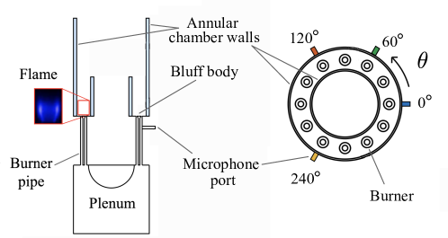
Figure 1: Side and top views of the experimental setup of the annular combustor. Adapted from Faure-Beaulieu et al. (2021b).

We use the experimental data of Faure-Beaulieu et al. (2021a) and Indlekofer et al. (2022). The experimental setup (Figure 1) consists of an annular combustor with twelve equally-spaced burners with premixed flames, which are fuelled with a mixture of 70/30% H₂/CH₄ by power. The operating conditions are atmospheric, and the thermal power is fixed at 72 kW. The equivalence ratios considered are $\Phi=\{0.4875,0.5125,0.5375,0.5625\}$. When $\Phi>0.5$ the system is thermoacoustically unstable with self-sustained oscillations that peak at approximately 1090 Hz (Indlekofer et al., 2022). The acoustic pressure data was recorded at a sampling rate of 51.2 kHz by Kulite pressure transducers (XCS-093-05D) at four azimuthal locations $\theta=\{0^{\circ},60^{\circ},120^{\circ},240^{\circ}\}$.

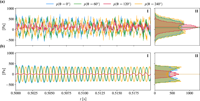
Figure 2: Pressure at the four measurement locations with equivalence ratio $\Phi=0.5125$ (thermoacoustically unstable configuration). (a) Raw experimental data, i.e., the observables, and (b) post-processed data, which is briefly referred to as the truth. (I) Time series of the fast-varying oscillations, and (II) histogram of the acoustic pressure in the time window for data assimilation, $t\in[0.5,0.85]$. The horizontal lines in (II) indicate the mean of the histograms. The thermoacoustic limit cycle is a standing acoustic mode with a nodal line near $\theta=120^{\circ}$ (mono-modal histogram).

Figure 2 shows the time series and histograms of the raw and post-processed experimental data at $\Phi=0.5125$ (Figure 2a,b). The pressure measurements have a mean value that is different from zero because of large-scale flow structures, which are not correlated to the thermoacoustic dynamics. The non-zero mean pressure is referred to as “measurement bias”, as further explained in §3.1. In a digital twin that is coupled with sensors’ measurements in real time, the data are the raw pressure signals that are assimilated into the low-order model (Figure 2a). Because the raw pressure contains aleatoric noise, measurement bias, and turbulent flow fluctuations, we refer to the post-processed data (Figure 2b) as the “presumed ground truth” or “presumed acoustic state”, that is, the physical acoustic state that is the presumed target prediction.

2.2 A qualitative and physics-based low-order model

The dynamics of the azimuthal acoustics can be qualitatively modelled by a one-dimensional wave-like equation (e.g., Faure-Beaulieu and Noiray, 2020; Indlekofer et al., 2022)

$$\dfrac{\partial^{2}p}{\partial t^{2}}+\zeta\dfrac{\partial p}{\partial t}-\left[1+\epsilon\cos{\left(2(\theta-\Theta_{\epsilon})\right)}\right]\dfrac{c^{2}}{r^{2}}\dfrac{\partial^{2}p}{\partial\theta^{2}}=(\gamma-1)\dfrac{\partial\dot{q}}{\partial t},$$ (1)

$$\text{with}\quad(\gamma-1)\dfrac{\partial\dot{q}}{\partial t}=\beta\left[1+c_{2}\cos{(2(\theta-\Theta_{\beta}))}\right]p-\kappa p^{3},$$ (2)

where $p$ is the acoustic pressure; $\zeta$ is the acoustic damping; $c$ is the speed of sound; $r$ is the mean radius of the annulus; $\gamma$ is the heat capacity ratio; $\epsilon$, and $\Theta_{\epsilon}$ are the amplitude and phase of the reactive symmetry, respectively (Indlekofer et al., 2022); and $\dot{q}$ is the coherent component of the fluctuations of the heat release rate (Noiray, 2017), which is divided into a nonlinear cubic term, which models the saturation of the flame response weighted by the parameter $\kappa$; and a linear response to the acoustic perturbations, which is weighted by the heat release strength $\beta$, the resistive asymmetry intensity, $c_{2}$, and direction of maximum root mean square acoustic pressure, $\Theta_{\beta}$. The flame response model (2) is an accurate approximation in the vicinity of a Hopf bifurcation (e.g., Lieuwen, 2003; Noiray, 2017). To further reduce the complexity of (2), we project the acoustic pressure on the degenerate pair of eigenmodes of the homogeneous wave equation (Noiray et al., 2011; Noiray and Schuermans, 2013b; Magri et al., 2023)

$$p(t,\theta)=\eta_{a}(t)\cos\theta+\eta_{b}(t)\sin\theta,$$ (3)

where $\eta_{a}$ and $\eta_{b}$ are the acoustic velocity amplitudes. Substituting (3) into (1) and averaging yield the governing equations, which consist of a set of nonlinearly coupled oscillators

$$\ddot{\eta}_{a}=- \omega^{2}\left[\eta_{a}\left(1+\frac{\epsilon}{2}\cos{(2\Theta_{\epsilon})}\right)+\eta_{b}\frac{\epsilon}{2}\sin{(2\Theta_{\epsilon})}\right]+$$ (4a)

$$\dot{\eta}_{a}\left[2\nu+\frac{c_{2}\beta}{2}\cos{(2\Theta_{\beta})}-\frac{3\kappa}{4}\left(3\eta_{a}^{2}+\eta_{b}^{2}\right)\right]+\dot{\eta}_{b}\left[\frac{c_{2}\beta}{2}\sin{(2\Theta_{\beta})}-\frac{3}{2}\kappa\eta_{b}\eta_{a}\right]$$

$$\ddot{\eta}_{b}=- \omega^{2}\left[\eta_{b}\left(1-\frac{\epsilon}{2}\cos{(2\Theta_{\epsilon})}\right)+\eta_{a}\frac{\epsilon}{2}\sin{(2\Theta_{\epsilon})}\right]+$$ (4b)

$$\dot{\eta}_{b}\left[2\nu-\frac{c_{2}\beta}{2}\cos{(2\Theta_{\beta})}-\frac{3\kappa}{4}\left(3\eta_{b}^{2}+\eta_{a}^{2}\right)\right]+\dot{\eta}_{a}\left[\frac{c_{2}\beta}{2}\sin{(2\Theta_{\beta})}-\frac{3}{2}\kappa\eta_{b}\eta_{a}\right]$$

where $\nu=(\beta-\zeta)/2$ is the linear growth rate of the pressure amplitude in absence of asymmetries, i.e., when $c_{2}=0$ (Indlekofer et al., 2022). Equation (4) can be written in a compact notation with a nonlinear state-space formulation

$$\left\{\begin{array}[]{rcl}\mathrm{d}\,{\bm{\mathit{\phi}}}&=&\mathcal{F}\left({\bm{\mathit{\phi,\alpha}}}\right)\mathrm{d}\,t\\[5.0pt] {\bm{\mathit{q}}}&=&\mathcal{M}({\bm{\mathit{\theta}}},{\bm{\mathit{\phi}}}),\end{array}\right.$$ (7)

where ${\bm{\mathit{\phi}}}=[\eta_{a};\dot{\eta}_{a};\eta_{b};\dot{\eta}_{b}]\in\mathbb{R}^{N_{\phi}}$ is the state vector; $\mathcal{F}:\mathbb{R}^{N_{\phi}}\rightarrow\mathbb{R}^{N_{\phi}}$ is the nonlinear operator that represents (4); and ${\bm{\mathit{\alpha}}}=[\nu;c_{2}\beta;\omega;\kappa;\epsilon;\Theta_{\beta};\Theta_{\epsilon}]\in\mathbb{R}^{N_{\alpha}}$ are the system’s parameters (the operator $[~{};~{}]$ indicates vertical concatenation, and we use column vectors throughout the manuscript). The vector ${\bm{\mathit{q}}}$ describes the model observables, which are the acoustic pressures at the azimuthal locations ${\bm{\mathit{\theta}}}=\{0^{\circ},60^{\circ},120^{\circ},240^{\circ}\}$. The model observables are computed through the measurement operator $\mathcal{M}:\mathbb{R}^{N_{\phi}}\rightarrow\mathbb{R}^{N_{q}}$, which maps the state variables into the observable space through (3).

3 Real-time data assimilation

Real-time data assimilation makes qualitatively models quantitatively accurate every time that sensors’ measurements (data) become available (Magri and Doan, 2020). At a measurement time $t_{k}$, the model’s state, ${\bm{\mathit{\phi}}}_{k}$, and parameters, ${\bm{\mathit{\alpha}}}_{k}$, are inferred by combining two sources of information, that is, the measurement, ${\bm{\mathit{d}}}_{k}$, and the model forecast, ${\bm{\mathit{q}}}_{k}$. A robust inference process must also filter out both epistemic and aleatoric uncertainties (§§3.1,3.2). The result of the assimilation is the analysis state (§§3.4,3.3), which provides a statistically optimal estimate of the physical quantity that we wish to predict, which is the truth ${\bm{\mathit{d}}}^{\dagger}_{k}$. As explained in §2.1, we define the post-processed acoustic pressure as the presumed ground truth (Figure 2). We drop the time subscript $k$ unless it is necessary for clarity.

3.1 Aleatoric and epistemic uncertainties

First, we discuss the statistical hypotheses on the aleatoric uncertainties. The aleatoric uncertainties contaminate the state and parameters as

$${\bm{\mathit{\phi}}}+{\bm{\mathit{\epsilon}}}_{\phi}={\bm{\mathit{\phi}}}^{\dagger},\quad{\bm{\mathit{\alpha}}}+{\bm{\mathit{\epsilon}}}_{\alpha}={\bm{\mathit{\alpha}}}^{\dagger},$$ (8)

where $\dagger$ indicates the true quantity (which is unknown). The aleatoric uncertainties are modelled as Gaussian distributions

$${\bm{\mathit{\epsilon}}}_{\phi}\sim\mathcal{N}({\bm{\mathit{0}}},\bm{\mathsf{C}}_{\phi\phi}),\quad{\bm{\mathit{\epsilon}}}_{\alpha}\sim\mathcal{N}({\bm{\mathit{0}}},\bm{\mathsf{C}}_{\alpha\alpha}),$$ (9)

where $\mathcal{N}({\bm{\mathit{0}}},\bm{\mathsf{C}})$ is a normal distribution with zero mean and covariance $\bm{\mathsf{C}}$. Second, we discuss model biases, which are epistemic uncertainties (Nóvoa et al., 2024). The model bias may arise from modelling assumptions and approximations in the operators $\mathcal{F}$ and $\mathcal{M}$. It is unknown a priori (colloquially, an “unknown unknown” (Nóvoa et al., 2024)). The bias is

$${\bm{\mathit{b}}}={\bm{\mathit{d}}}^{\dagger}-\mathbb{E}({\bm{\mathit{q}}}),$$ (10)

which is the expected difference between the true observable and the model observable. (If the model is unbiased, ${\bm{\mathit{d}}}^{\dagger}=\mathbb{E}({\bm{\mathit{q}}})$.) Hence, the bias-corrected model observable is

$${\bm{\mathit{y}}}={\bm{\mathit{q}}}+{\bm{\mathit{b}}}+{\bm{\mathit{\epsilon}}}_{q},$$ (11)

where ${\bm{\mathit{\epsilon}}}_{q}\sim\mathcal{N}({\bm{\mathit{0}}},\bm{\mathsf{C}}_{qq})$. The final model equations, which define the first source of information on the system, are

$$\left\{\begin{array}[]{rcl}\mathrm{d}\,{\bm{\mathit{\phi}}}&=&\mathcal{F}\left({\bm{\mathit{\phi+{\bm{\mathit{\epsilon}}}_{\phi},\alpha+{\bm{\mathit{\epsilon}}}_{\alpha}}}}\right)\mathrm{d}\,t\\[5.0pt] {\bm{\mathit{y}}}&=&\mathcal{M}({\bm{\mathit{\theta}}},{\bm{\mathit{\phi}}})+{\bm{\mathit{b}}}+{\bm{\mathit{\epsilon}}}_{q}\end{array}\right.$$ (14)

The set of equations (14) is not closed because we need a model for the model bias (§4).

The second source of information on the system is the data measured by the sensors. Experimental data are affected by both aleatoric noise and measurement biases (§2.1). The measurements at a time instant are

$${\bm{\mathit{d}}}+{\bm{\mathit{b}}}_{d}+{\bm{\mathit{\epsilon}}}_{d}={\bm{\mathit{d}}}^{\dagger},$$ (15)

where the measurement bias ${\bm{\mathit{b}}}_{d}$ is defined as

$${\bm{\mathit{b}}}_{d}=\mathbb{E}({\bm{\mathit{d}}})-{\bm{\mathit{d}}}^{\dagger}.$$ (16)

In the problem under investigation, ${\bm{\mathit{d}}}$ is the raw acoustic data, ${\bm{\mathit{d}}}^{\dagger}$ is is the post-processed data, and ${\bm{\mathit{b}}}_{d}$ is the non-zero mean of the raw data (see §2.1). The aleatoric noise affects the measurement as ${\bm{\mathit{\epsilon}}}_{d}\sim\mathcal{N}({\bm{\mathit{0}}},\bm{\mathsf{C}}_{dd})$. For simplicity, we assume that the measurement errors are statistically independent, i.e., $\bm{\mathsf{C}}_{dd}$ is a diagonal matrix with diagonal ${\bm{\mathit{\epsilon}}}_{d}$.

Both model and measurement biases are unknown a priori. To infer them, we analyse the residuals between the forecast and the observations, which are also known as innovations (Dee and Todling, 2000; Haimberger, 2007)

$${\bm{\mathit{i}}}={\bm{\mathit{d}}}-{\bm{\mathit{q}}}.$$ (17)

Hence, the expected value of the innovation is

$$\mathbb{E}({\bm{\mathit{i}}})={\bm{\mathit{b}}}_{d}+{\bm{\mathit{b}}},$$ (18)

i.e., the expected innovation is the sum of the measurement and model biases. The relation between the innovations ${\bm{\mathit{i}}}$ and the biases ${\bm{\mathit{b}}}$ and ${\bm{\mathit{b}}}_{d}$ will be essential for the design of the bias estimator in §4.

3.2 Augmented state-space formulation

We define the augmented state vector ${\bm{\mathit{\psi}}}=[{\bm{\mathit{\phi}}};{\bm{\mathit{\alpha}}};{\bm{\mathit{q}}}]$, which comprises the state variables, the thermoacoustic parameters and the model observables to formally have a linear measurement operator $\bm{\mathsf{M}}$, which simplifies the derivation of data assimilation methods (e.g., Nóvoa and Magri, 2022). The augmented form of the model (14) yields

$$\left\{\begin{array}[]{rcl}\mathrm{d}\,\begin{bmatrix}{\bm{\mathit{\phi}}}\\ {\bm{\mathit{\alpha}}}\\ {\bm{\mathit{q}}}\end{bmatrix}&=&\begin{bmatrix}\mathcal{F}({\bm{\mathit{\phi}}}+{\bm{\mathit{\epsilon}}}_{\phi},{\bm{\mathit{\alpha}}}+{\bm{\mathit{\epsilon}}}_{\alpha})\\ {\bm{\mathit{0}}}_{N_{\alpha}}\\ {\bm{\mathit{0}}}_{N_{q}}\end{bmatrix}{\mathrm{d}\,t}\\[20.00003pt] {\bm{\mathit{y}}}&=&{\bm{\mathit{q}}}+{\bm{\mathit{b}}}+{\bm{\mathit{\epsilon}}}_{q}\end{array}\right.\quad\leftrightarrow\quad\left\{\begin{array}[]{rcl}\mathrm{d}\,{\bm{\mathit{\psi}}}&=&\bm{\mathsf{F}}\left({\bm{\mathit{\psi}}}+{\bm{\mathit{\epsilon}}}_{\psi}\right){\mathrm{d}\,t}\\[10.00002pt] {\bm{\mathit{y}}}&=&\bm{\mathsf{M}}{\bm{\mathit{\psi}}}+{\bm{\mathit{b}}}+{\bm{\mathit{\epsilon}}}_{q}\end{array}\right.$$ (23)

where $\bm{\mathsf{F}}({\bm{\mathit{\psi}}})$ and ${\bm{\mathit{\epsilon}}}_{\psi}$ are the augmented nonlinear operator and aleatoric uncertainties, respectively; $\bm{\mathsf{M}}=\left[\bm{\mathsf{0}}~{}\big{|}~{}\mathbb{I}_{N_{q}}\right]$ is the linear measurement operator, which consists of the vertical concatenation of a matrix of zeros, $\bm{\mathsf{0}}\in\mathbb{R}^{N_{q}\times(N_{\phi}+N_{\alpha})}$, and the identity matrix, $\mathbb{I}_{N_{q}}\in\mathbb{R}^{N_{q}\times N_{q}}$; and ${\bm{\mathit{0}}}_{N_{\alpha}}$ and ${\bm{\mathit{0}}}_{N_{q}}$ are vectors of zeros (because the parameters are constant in time, and ${\bm{\mathit{q}}}$ is not integrated in time but it is only computed at the analysis step).

3.3 Stochastic ensemble framework

Under the Gaussian assumption, the inverse problem of finding the states, ${\bm{\mathit{\phi}}}$, and parameters, ${\bm{\mathit{\alpha}}}$, given some observations, ${\bm{\mathit{d}}}$, would be be solved by the Kalman filter equations if the operator $\mathcal{F}$ were linear (Kalman, 1960). Thermoacoustic oscillations, however, have nonlinear dynamics (see (1)). Stochastic ensemble methods are suitable for nonlinear systems because they do not require to propagate the covariance, in contrast to other sequential methods, e.g., the extended Kalman filter (Evensen, 2009; Nóvoa and Magri, 2022). Stochastic ensemble filters track in time $m$ realizations of the augmented state ${\bm{\mathit{\psi}}}_{j}$ to estimate the mean and covariance, respectively

$$\mathbb{E}({\bm{\mathit{\psi}}}) \approx\bar{{\bm{\mathit{\psi}}}}=\dfrac{1}{m}\sum^{m}_{j=1}{{\bm{\mathit{\psi}}}_{j}}$$ (24a)

$$\bm{\mathsf{C}}_{\psi\psi}=\begin{bmatrix}\bm{\mathsf{C}}_{\phi\phi}&\bm{\mathsf{C}}_{\phi\alpha}&\bm{\mathsf{C}}_{\phi q}\\ \bm{\mathsf{C}}_{\alpha\phi}&\bm{\mathsf{C}}_{\alpha\alpha}&\bm{\mathsf{C}}_{\alpha q}\\ \bm{\mathsf{C}}_{q\phi}&\bm{\mathsf{C}}_{q\alpha}&\bm{\mathsf{C}}_{qq}\\ \end{bmatrix} \approx\dfrac{1}{m-1}\sum^{m}_{j=1}({\bm{\mathit{\psi}}}_{i}-\bar{{\bm{\mathit{\psi}}}})\otimes({\bm{\mathit{\psi}}}_{i}-\bar{{\bm{\mathit{\psi}}}}),$$ (24b)

where $\otimes$ is the dyadic product. (Because the forecast operator $\mathcal{F}$ is nonlinear, the Gaussian prior may not remain Gaussian after the model forecast, and $\mathbb{E}(\mathcal{F}({\bm{\mathit{\psi}}}))\neq\mathcal{F}(\bar{{\bm{\mathit{\psi}}}})$. However, the time between analyses $\Delta t_{\mathrm{d}}$ is assumed small enough such that the Gaussian distribution is not significantly distorted (Evensen, 2009; Yu et al., 2019b).)

Finally, we approximate the model bias (10) and measurement bias (18) with the ensemble statistics

$${\bm{\mathit{b}}} \approx{\bm{\mathit{d}}}^{\dagger}-\bm{\mathsf{M}}\bar{{\bm{\mathit{\psi}}}},$$ (25)

$${\bm{\mathit{b}}}_{d} \approx{\bm{\mathit{d}}}^{\dagger}-\bar{{\bm{\mathit{d}}}}.$$ (26)

Hence, the innovation of the ensemble mean can be approximated as

$$\bar{{\bm{\mathit{i}}}}={\bm{\mathit{d}}}-\bm{\mathsf{M}}\bar{{\bm{\mathit{\psi}}}}\approx{\bm{\mathit{b}}}_{d}+{\bm{\mathit{b}}}.$$ (27)

3.4 The bias-regularized ensemble Kalman filter

The objective function in a bias-regularized data assimilation framework contains three norms (Nóvoa et al., 2024)

$$\mathcal{J}({\bm{\mathit{\psi}}}_{j})= \left\|{\bm{\mathit{\psi}}}_{j}-{\bm{\mathit{\psi}}}_{j}^{\mathrm{f}}\right\|^{2}_{\bm{\mathsf{C}}^{\mathrm{f}^{-1}}_{\psi\psi}}+\left\|{{\bm{\mathit{y}}}}_{j}-{\bm{\mathit{d}}}_{j}\right\|^{2}_{\bm{\mathsf{C}}^{-1}_{dd}}+\gamma\left\|{\bm{\mathit{b}}}_{j}\right\|^{2}_{\bm{\mathsf{C}}^{-1}_{bb}},\quad\mathrm{for}\quad j=0,\dots,m-1$$ (28)

where the superscript ‘f’ indicates ‘forecast’; the operator $\left\|\cdot\right\|^{2}_{\bm{\mathsf{C}}^{-1}}$ is the $L_{2}$-norm weighted by the semi-positive definite matrix ${\bm{\mathsf{C}}^{-1}}$; $\gamma\geq 0$ is a user-defined bias regularization factor; and ${\bm{\mathit{b}}}_{j}$ is the model bias of each ensemble member. For simplicity, we define the bias in the ensemble mean, such that ${\bm{\mathit{b}}}_{j}={\bm{\mathit{b}}}$ for all $j$ (which we estimate with an echo state network §4) (Nóvoa et al., 2024). From left to right, the norms on the right-hand-side of (28) measure (1) the spread of the ensemble prediction, (2) the distance between the bias-corrected estimate and the observables, and (3) the model bias. The analytical solution of the bias-regularized ensemble Kalman filter (r-EnKF) in (29), which globally minimizes the cost function (28) with respect to ${\bm{\mathit{\psi}}}_{j}$, is

$${\bm{\mathit{\psi}}}_{j}^{\mathrm{a}} ={\bm{\mathit{\psi}}}_{j}^{\mathrm{f}}+\bm{\mathsf{K}}_{\mathrm{r}}\left[\left(\mathbb{I}+\bm{\mathsf{J}}\right)\left({\bm{\mathit{d}}}_{j}+{\bm{\mathit{b}}}_{d}^{\mathrm{f}}-{\bm{\mathit{y}}}_{j}^{\mathrm{f}}\right)-\gamma\bm{\mathsf{C}}_{dd}\bm{\mathsf{C}}^{-1}_{bb}\bm{\mathsf{J}}{\bm{\mathit{b}}}^{\mathrm{f}}\right],\quad j=0,\dots,m-1$$ (29a)

with

$$\bm{\mathsf{K}}_{\mathrm{r}}=\bm{\mathsf{C}}_{\psi\psi}^{\mathrm{f}}\bm{\mathsf{M}}^{\mathrm{T}}\left[\bm{\mathsf{C}}_{dd}+(\mathbb{I}+\bm{\mathsf{J}})\bm{\mathsf{M}}\bm{\mathsf{C}}_{\psi\psi}^{\mathrm{f}}\bm{\mathsf{M}}^{\mathrm{T}}(\mathbb{I}+\bm{\mathsf{J}})^{\mathrm{T}}+\gamma\bm{\mathsf{C}}_{dd}\bm{\mathsf{C}}^{-1}_{bb}\bm{\mathsf{J}}\bm{\mathsf{M}}\bm{\mathsf{C}}_{\psi\psi}^{\mathrm{f}}\bm{\mathsf{M}}^{\mathrm{T}}{\bm{\mathsf{J}}}^{\mathrm{T}}\right]^{-1},$$ (29b)

where ‘a’ stands for ‘analysis’, i.e, the optimal state of the assimilation; we assimilate each ensemble member with a different ${\bm{\mathit{d}}}_{j}\sim\mathcal{N}({\bm{\mathit{d}}},\bm{\mathsf{C}}_{dd})$ to avoid covariance underestimation in ensemble filters (Burgers et al., 1998); $\bm{\mathsf{K}}_{\mathrm{r}}$ is the regularized Kalman gain matrix; and $\bm{\mathsf{J}}=\mathrm{d}\,{\bm{\mathit{b}}}/\mathrm{d}\,\bm{\mathsf{M}}{\bm{\mathit{\psi}}}$ is the Jacobian of the bias estimator. Formulae 29 generalize the analytical solutions of Nóvoa et al. (2024) to the case of biased measurement. We prescribe $\bm{\mathsf{C}}_{dd}=\bm{\mathsf{C}}_{bb}$ because the model bias is defined in the observable space. We use $\gamma$ to tune the norm of the bias in (28) (Nóvoa et al., 2024). The optimal state and parameters are

$$\begin{bmatrix}{\bm{\mathit{\phi}}}_{j}^{\mathrm{a}}\\[10.00002pt] {\bm{\mathit{\alpha}}}_{j}^{\mathrm{a}}\end{bmatrix}=\begin{bmatrix}{\bm{\mathit{\phi}}}_{j}^{\mathrm{f}}\\[10.00002pt] {\bm{\mathit{\alpha}}}_{j}^{\mathrm{f}}\end{bmatrix}+\overbrace{\begin{bmatrix}\bm{\mathsf{C}}_{\phi q}^{\mathrm{f}}\\[10.00002pt] \bm{\mathsf{C}}_{\alpha q}^{\mathrm{f}}\end{bmatrix}\left\{\bm{\mathsf{C}}_{dd}+(\mathbb{I}+\bm{\mathsf{J}})\bm{\mathsf{C}}_{qq}^{\mathrm{f}}(\mathbb{I}+\bm{\mathsf{J}})^{\mathrm{T}}+\gamma\bm{\mathsf{J}}\bm{\mathsf{C}}_{qq}^{\mathrm{f}}{\bm{\mathsf{J}}}^{\mathrm{T}}\right\}^{-1}}^{\mathrm{Regularized\,Kalman\,gain,\,\bm{\mathsf{K}}_{\mathrm{r}}}}\dots$$

$$\dots\Big{[}\left(\mathbb{I}+\bm{\mathsf{J}}\right)\overbrace{\left({\bm{\mathit{d}}}_{j}+{\bm{\mathit{b}}}_{d}^{\mathrm{f}}-{\bm{\mathit{y}}}_{j}^{\mathrm{f}}\right)}^{\mathrm{Corrected\,innovation}}-\gamma\bm{\mathsf{J}}{\bm{\mathit{b}}}^{\mathrm{f}}\Big{]}$$ (30)

The r-EnKF defines a ‘good’ analysis from a biased model if the unbiased state ${\bm{\mathit{y}}}$ matches the truth, and the model bias ${\bm{\mathit{b}}}$ is small relative to the truth. The underlying assumptions of this work are that (i) our low-order model is qualitatively accurate such that the model bias ${\bm{\mathit{b}}}^{\mathrm{f}}$ has a small norm; and (ii) the sensors are properly calibrated. In the limiting case when the assimilation framework is unbiased (i.e., ${\bm{\mathit{b}}}={\bm{\mathit{0}}}$, and ${\bm{\mathit{b}}}_{d}={\bm{\mathit{0}}}$), the r-EnKF (3.4) becomes the bias-unregularized EnKF (A).

4 Reservoir computing for inferring model and measurement biases

To apply the r-EnKF (3.4) we must provide an estimate of the model bias and the measurement bias. We employ an echo state network (ESN) for this task. ESNs are suitable for real-time data assimilation because (i) they are recurrent neural networks, i.e., they are designed to learn temporal dynamics in data; (ii) they are based on reservoir computing, hence they are universal approximators (Grigoryeva and Ortega, 2018); (iii) they are general nonlinear auto-regressive models (Aggarwal, 2018); and (iv) training an ESN consists of solving a linear regression problem, which provides a global minimum without back propagation. In this work, we generalize the implementation of Nóvoa et al. (2024) to account for both the model and measurement biases (§4.1). We propose a training dataset generation based on time-series correlation (§4.2).

4.1 Echo state network architecture and state-space formulation

We propose an ESN that simultaneously estimates ${\bm{\mathit{b}}}^{\mathrm{f}}$ and ${\bm{\mathit{b}}}_{d}^{\mathrm{f}}$ (where ‘f’ indicates that the biases are forecast quantities, which are equivalent to the actual biases at convergence). Importantly, the biases ${\bm{\mathit{b}}}$ and ${\bm{\mathit{b}}}_{d}$ are not directly measurable in real-time, but we have access to the innovation, which is linked to the biases through (27). Once we have information on the innovation and the model bias (the measurement bias), we can estimate the measurement bias (the model bias) through Eq. 27.

Figure 3a represents pictorially the proposed ESN at time $t_{k}$, with its three main components: (i) the input data, which are the mean analysis innovations, i.e, $\bar{{\bm{\mathit{i}}}}^{\mathrm{a}}_{k}={\bm{\mathit{d}}}_{k}-\bm{\mathsf{M}}\bar{{\bm{\mathit{\psi}}}}_{k}^{\mathrm{a}}$; (ii) the reservoir, which is a high-dimensional state is characterized by the sparse reservoir matrix $\bm{\mathsf{W}}\in\mathbb{R}^{N_{r}\times N_{r}}$ and vector ${\bm{\mathit{r}}}_{k}\in\mathbb{R}^{N_{r}}$ ($N_{r}\gg N_{q}$ is the number of neurons in the reservoir states); and (iii) the outputs, which are the mean innovation and the model bias at the next time step, i.e., $\bar{{\bm{\mathit{i}}}}^{\mathrm{f}}_{k+1}$ and ${\bm{\mathit{b}}}^{\mathrm{f}}_{k+1}$. The inputs to the network are a subset of the output (i.e., the innovation only). The sparse input matrix $\bm{\mathsf{W}}_{\mathrm{in}}\in\mathbb{R}^{N_{r}\times(N_{q}+1)}$ maps the physical state into the reservoir, and the output matrix $\bm{\mathsf{W}}_{\mathrm{out}}\in\mathbb{R}^{N_{q}\times(N_{r}+1)}$ maps the reservoir state back to the physical state.

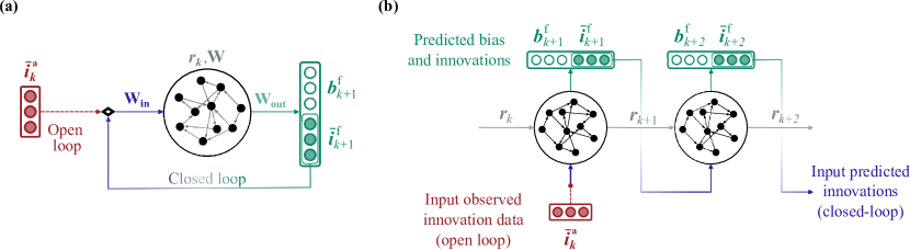
Figure 3: Schematic representation of the proposed echo state network architecture for model bias and innovation prediction. (a) Compact architecture showing the open-loop and closed-loop configurations; and (b) unfolded architecture starting at an analysis step is at $t_{k}$, in which there is one open-loop step followed by a closed-loop forecast. In open loop the input to the ESN is the analysis mean innovation $\bar{{\bm{\mathit{i}}}}^{\mathrm{a}}_{k}={\bm{\mathit{d}}}_{k}-\bm{\mathsf{M}}\bar{{\bm{\mathit{\psi}}}}_{k}^{\mathrm{a}}$, i.e., the difference between the raw acoustic pressure data and the analysis model estimate. The outputs from the ESN are (i) the innovation at the next time step $\bar{{\bm{\mathit{i}}}}^{\mathrm{f}}_{k+1}$ (which becomes the input to the next time step in closed loop configuration); and (ii) the model bias ${\bm{\mathit{b}}}^{\mathrm{f}}_{k+1}$, i.e., an estimate of the difference between the presumed acoustic state ${\bm{\mathit{d}}}_{k+1}^{\dagger}$ and the model estimate ${\bm{\mathit{q}}}_{k+1}$.

Further, Figure 3a shows the two forecast settings of the echo state network: open-loop, which is performed when data on the innovations are available, and the closed-loop, in which the ESN runs autonomously using the output as the input in the next time step. Figure 3b shows the unfolded architecture starting at time $t_{k}$ when observations of the innovations are available (i.e., at the analysis step). At this time, the reservoir is re-initialized with the analysis innovations such that the input to the ESN is $\bar{{\bm{\mathit{i}}}}^{\mathrm{a}}_{k}={\bm{\mathit{d}}}_{k}-\bm{\mathsf{M}}\bar{{\bm{\mathit{\psi}}}}_{k}^{\mathrm{a}}$. From this, the ESN estimates at the next time step $t_{k+1}$ the model bias and the innovation $\bar{{\bm{\mathit{i}}}}^{\mathrm{f}}_{k+1}$, which is used as initial condition in the subsequent forecast step. Mathematically, the equations that forecast the model bias and mean innovation in time are

$$[{\bm{\mathit{b}}}_{k+1}^{\mathrm{f}};\bar{{\bm{\mathit{i}}}}^{\mathrm{f}}_{k+1}] =\bm{\mathsf{W}}_{\mathrm{out}}\left[{\bm{\mathit{r}}}_{k+1};1\right]$$

$${\bm{\mathit{r}}}_{k+1} =\textrm{tanh}\left(\sigma_{\mathrm{in}}\bm{\mathsf{W}}_{\mathrm{in}}\left[\bar{{\bm{\mathit{i}}}}^{\star}_{k}\odot{\bm{\mathit{g}}};\delta_{\mathrm{r}}\right]+\rho\bm{\mathsf{W}}{\bm{\mathit{r}}}_{k}\right),$$ (31)

where $\bar{{\bm{\mathit{i}}}}^{\star}=\bar{{\bm{\mathit{i}}}}^{\mathrm{a}}$ in open loop and $\bar{{\bm{\mathit{i}}}}^{\star}=\bar{{\bm{\mathit{i}}}}^{\mathrm{f}}$ in closed loop; the ${\tanh(\cdot)}$ operation is performed element-wise; the operator $\odot$ is the Hadamard product, i.e., component-wise multiplication; and ${\bm{\mathit{g}}}=[g_{1};\dots;g_{2N_{q}}]$ is the input normalizing term with $g_{q}^{-1}=\max{({\bm{\mathit{u}}}_{q})}-\min{({\bm{\mathit{u}}}_{q})}$, i.e., $g_{q}^{-1}$ is the range of the $q^{\mathrm{th}}$ component of the training data $\bm{\mathsf{U}}$; $\delta_{\mathrm{r}}$ is a constant used for breaking the symmetry of the ESN (we set $\delta_{\mathrm{r}}=0.1$) (Huhn and Magri, 2020). We define $\bm{\mathsf{W}}_{\mathrm{in}}$ and $\bm{\mathsf{W}}$ as sparse and randomly generated, with a connectivity of 3 neurons (see Jaeger and Haas, 2004, for details). We compute the matrix $\bm{\mathsf{W}}_{\mathrm{out}}$ during the training.

Lastly, the r-EnKF equations (29) require the definition of the Jacobian of the bias estimator at the analysis step. Because at the analysis step the ESN inputs the analysis innovations with an open-loop step (see Figure 3b), the Jacobian of the bias estimator is equivalent to the negative Jacobian of the echo state network in open loop configuration (see B).

4.2 Training the network

During training, the ESN is in open-loop configuration (Figure 3a). The inputs to the reservoir are the training dataset $\bm{\mathsf{U}}=\left[{\bm{\mathit{u}}}_{0}\,|\dots|\,{\bm{\mathit{u}}}_{N_{\mathrm{tr}}-1}\right]$, in which each time component ${\bm{\mathit{u}}}_{k}=[{\bm{\mathit{b}}}_{\mathrm{u}}(t_{k});{{\bm{\mathit{i}}}}_{\mathrm{u}}(t_{k})]$, the subscript ‘u’ indicates training data, and the operator $[~{}|~{}]$ indicates horizontal concatenation. Although we have information from the experimental data to train the network, the optimal parameters of the thermoacoustic system are unknown. Thus, we do not know a priori the model bias and measurement bias. Selecting an appropriate training dataset is key to obtaining a robust ESN, which can estimate the model bias and innovations. We create a set of $L$ guesses on the bias and innovations from a single realization of the experimental data, which means that the ESN is not trained with the ‘true’ bias (which is an unknown quantity in real time). The training data is generated from the experimental data as detailed in C. In summary, the procedure is as follows.

1. Take measurements for a training time window $t_{\mathrm{train}}$ of acoustic pressure data $\bm{\mathsf{D}}_{\mathrm{u}}$, and estimate $\bm{\mathsf{D}}^{\dagger}_{\mathrm{u}}$ by filtering the power spectral density of $\bm{\mathsf{D}}$ (see §2).

2. Generate $L$ model estimates $\bm{\mathsf{Q}}_{\mathrm{u},l}$ of the acoustic pressure from (4) with randomly generated parameters, and correlate in time each $\bm{\mathsf{Q}}_{\mathrm{u},l}$ with $\bm{\mathsf{D}}_{\mathrm{u}}$.

3. Compute the training model bias as $\bm{\mathsf{B}}_{\mathrm{u},l}=\bm{\mathsf{D}}^{\dagger}_{\mathrm{u}}-\bm{\mathsf{Q}}_{\mathrm{u},l}$ and the training innovations as $\bm{\mathsf{I}}_{\mathrm{u},l}=\bm{\mathsf{D}}_{\mathrm{u}}-\bm{\mathsf{Q}}_{\mathrm{u},l}.$

4. Apply data augmentation to improve the network’s adaptivity in a real-time assimilation framework.

The total number of training time series in the proposed training method is $2L$. Training the ESN consists of finding the elements in $\bm{\mathsf{W}}_{\mathrm{out}}$, which minimize the distance between the outputs obtained from an open-loop forecast step of the training data (the features) to the training data at the following time step (the labels). This minimization is solved by ridge regression of the linear system (Lukoševičius, 2012)

$$\left(\sum_{l=0}^{2L-1}\bm{\mathsf{R}}^{\,}_{l}\bm{\mathsf{R}}_{l}^{\mathrm{T}}+\lambda\,\mathbb{I}_{N_{r}+1}\right)\bm{\mathsf{W}}_{\mathrm{out}}^{\mathrm{T}}=\sum_{l=0}^{2L-1}\bm{\mathsf{R}}_{l}^{\,}\bm{\mathsf{U}}_{l}^{\mathrm{T}},$$ (32)

where $\lambda$ is the Tikhonov regularization parameter; and $\bm{\mathsf{R}}=\left[[{\bm{\mathit{r}}}_{0};1]\,|\dots|\,[{\bm{\mathit{r}}}_{N_{\mathrm{train}}-1};1]\right]$, with ${\bm{\mathit{r}}}_{0}={\bm{\mathit{0}}}$ and ${\bm{\mathit{r}}}_{k}$ are obtained with (4.1) using the innovations of the training set as inputs. The summations over $2L$ can be performed in parallel to minimize computational costs. Finally, we tune the hyperparameters of the echo state network, i.e., the spectral radius $\rho$, the input scaling $\sigma_{\mathrm{in}}$ and the Tikhonov regularization parameter $\lambda$. We use a recycle validation strategy with Bayesian optimization for the hyperparameter selection (see Racca and Magri, 2021).

5 Performance of the real-time digital twin

The real-time digital twin has four components: (i) data from sensors (§2.1) (ii) the physics-based low order model (§2.2), (iii) the echo state network to infer the model and measurement biases (§4), and (iv) the real-time and bias-regularized data assimilation method (§3.4) to twin sensors’ data with the low-order model to infer the state and model parameters. We investigate the capability of the proposed real-time digital twin to predict autonomously the dynamics of azimuthal thermoacoustic oscillations. We analyse the digital twin’s performance with respect to established methods: the bias-unregularized ensemble Kalman filter (EnKF) (Nóvoa and Magri, 2022), which is suitable for real-time assimilation; and Langevin-based regression (Indlekofer et al., 2022), which is suitable for offline assimilation. The hyperparameters used to train the ESN, and the assimilation parameters are reported in D.

5.1 Time-accurate prediction

We focus our analysis on the equivalence ratio $\Phi=0.5125$, which is a thermoacoustically unstable system. Figure 4 shows the time evolution of the acoustic pressure at $\theta=60^{\circ}$. The digital twin is initialized during a short time window up to $0.5$ s. After this, data points from the raw experimental data (red dots) are assimilated every $\Delta t_{\mathrm{d}}=5.86\cdot 10^{-4}$ seconds, which corresponds to approximately $0.64$ data points per acoustic period. At a time instant, the measurement (the data point, red dot) is assimilated into the model, which adaptively updates itself through the r-EnKF and bias estimators (§§3.4,4). After that, the state and model parameters have been updated, the low-order model (7) evolves autonomously until the next data point becomes available. This process mimics a stream of data coming from sensors on the fly. We assimilate 600 measurements during the assimilation window of $0.15$ seconds, the model runs autonomously without seeing more data ($t>0.85$ s).

First, we analyse the performance of the bias-unregularized filter (EnKF) on state estimation (Figure 4a) with the corresponding parameter inference shown in Figure 5 (dashed lines).

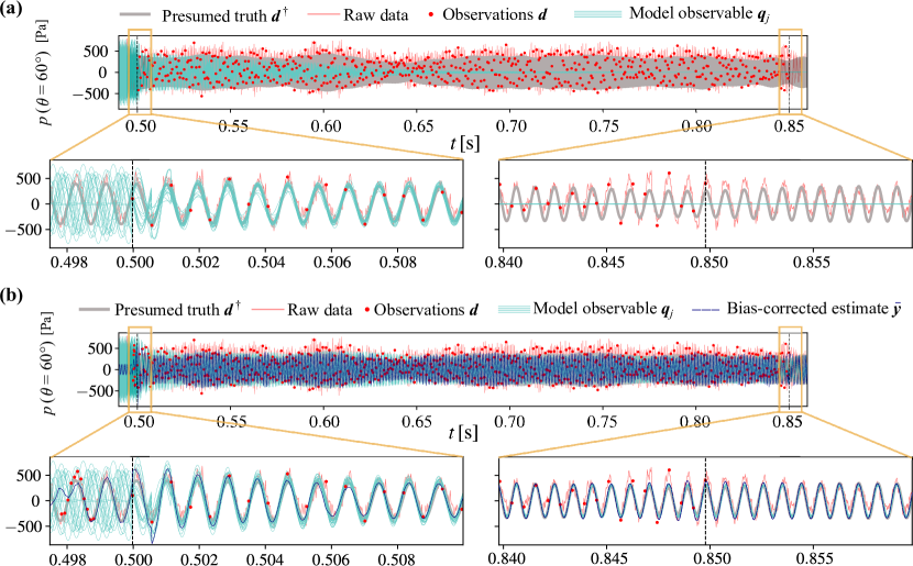
Figure 4: Real-time digital twin at $\Phi=0.5125$. Time evolution of the thermoacoustic pressure (in Pa) at $\theta=60^{\circ}$ using (a) the bias-unregularized EnKF and (b) the proposed bias-regularized EnKF (r-EnKF). Comparison between the presumed ground truth (thick grey line), the raw data (thick red line), the prediction from the ensemble filter (cyan lines), and in (b) the bias-corrected mean estimate (navy dashed line). The close ups show the start and end of the assimilation window, which is indicated by the vertical dashed lines. The observations are show in red circles.

Figure 5: Thermoacoustic parameters with the bias-unregularized EnKF (dashed) and the bias-regularized r-EnKF (solid). The lines and shaded areas indicate the ensemble mean and standard deviation, respectively. $\Phi=0.5125$.

Although the system has a self-sustained oscillation, the bias-unregularized filter converges towards an incorrect solution, that is, a fixed point. On the other hand, the bias-regularized filter (r-EnKF) successfully learns the thermoacoustic model. Second, the r-EnKF filters out aleatoric noise and turbulent fluctuations. These fluctuations are the difference between the amplitudes of the raw data, which are the input to the digital twin, and the post-processed data, which are the hidden state that we wish to uncover and predict (the presumed acoustic state), of up to approximately 200 Pa (close-ups at the end of assimilation in Figure 4). Third, after assimilation, the r-EnKF predicts the thermoacoustic limit cycle beyond the assimilation window. This means that the digital twin has learnt an accurate model of the system, which generalizes beyond the assimilation. The ensemble model observables ${\bm{\mathit{q}}}_{j}$ and bias-corrected ensemble mean $\bar{{\bm{\mathit{y}}}}=\bar{{\bm{\mathit{q}}}}+{\bm{\mathit{b}}}$ are almost identical at convergence in Figure 4b, which means that the magnitude of the model bias is small (approximately 20 Pa in amplitude, see Figure 7). Fourth, the r-EnKF infers the optimal system’s thermoacoustic parameters, which are seven in this model (Figure 5). The ensemble parameters at $t=0$ in Figure 5 are initialized on physical ranges from the physical parameters used in the literature, which are computed by Langevin regression in (Indlekofer et al., 2022). From inspection of the optimal parameters, we can draw physical conclusions: (i) the parameters of the literature are not the optimal parameters of the model; (ii) the linear growth rate, $\nu$, angular frequency, $\omega$, the heat release strength weighted by the symmetry intensity, $c_{2}\beta$, and the phase of the reactive symmetry, $\Theta_{\epsilon}$, do not significantly vary at regime, which means that these parameters are constants and do not depend on the state; and (iii) the nonlinear parameter, $\kappa$, the amplitude of the reactive symmetry, $\epsilon$, and the direction of asymmetry, $\Theta_{\beta}$ have temporal variations that follow the modulation of the pressure signal envelope (Figure 5). Physically, this means that the optimal deterministic system that represents azimuthal instabilities is a time-varying parameter system (Durbin and Koopman, 2012). By inferring time-varying parameters, we derive a deterministic system that does not require stochastic modelling. We further analyse the thermoacoustic parameters for all the equivalence ratios in Figures 9 and 10.

To summarize, the presence of model biases and measurement biases makes the established bias-unregularized ensemble Kalman filter fail to uncover and predict the physical state from noisy data. In contrast, the bias-regularized filter (r-EnKF) infers the state, parameters, model bias, and measurement bias, which enable a time-accurate and physical prediction beyond the assimilation window.

5.2 Statistics and biases

We analyse the uncertainty and the statistics of the time series (§5.1) generated by the real-time digital twin. To do so, we define the normalized root-mean square (RMS) error of two time series ${\bm{\mathit{w}}},{\bm{\mathit{z}}}$ with $N_{q}$ dimensions and $N_{t}$ time steps as

$$\mathrm{RMS}({\bm{\mathit{w}}},{\bm{\mathit{z}}}) =\sqrt{\dfrac{\sum_{q}\sum_{k}\left({w}_{q}(t_{k})-{z}_{q}(t_{k})\right)^{2}}{\sum_{q}\sum_{k}\left({w}_{q}(t_{k})\right)^{2}}},\quad\mathrm{for}\;\begin{array}[]{l}q=0,\dots,N_{q}-1,\\[5.0pt] k=0,\dots,N_{t}-1.\end{array}$$ (35)

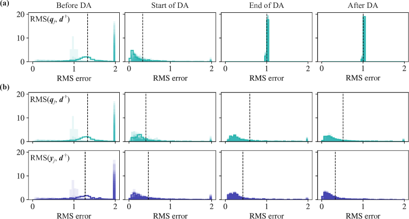
Figure 6: Normalized RMS errors between the presumed ground truth and the model prediction (cyan) and between the presumed ground truth and the bias-corrected prediction (navy) with (a) the bias-unregularized EnKF and (b) the r-EnKF. The filled histograms show the RMS of each ensemble member, the thick lines show the RMS of the ensemble mean, and the vertical dashed line indicates the mean of the RSM error. The errors are computed at four stages of the assimilation: $t\in[0.49,0.50]$ (before DA), $t\in[0.50,0.51]$ (start of DA), $t\in[0.84,0.85]$ (end of DA), and $t\in[0.85,0.86]$ (after DA). $\Phi=0.5125$.

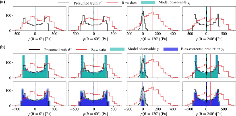
Figure 7: Histograms of the acoustic pressure after assimilation with (a) the bias-unregularized EnKF and (b) the r-EnKF, at the four observed azimuthal locations. Comparison between the presumed ground truth (black), the observations from raw data (red), the ensemble prediction (filled cyan) and its mean (dashed teal), and bias-corrected ensemble predictions (filled navy) and its mean (dashed light blue). The vertical lines indicate the mean of each of the distributions. $\Phi=0.5125$.

Figure 6 shows the RMS errors at four critical time instants in the assimilation process: before the data is assimilated (first column), which corresponds to the initialization of the digital twin; at the start and end of the data assimilation window (second and third columns, respectively); and after the data assimilation (fourth column), i.e., when the digital twin evolves autonomously to predict unseen dynamics (generalization). The inference of the model and measurement biases is key to obtaining a small generalization error. Although the bias-unregularized EnKF converges to an unphysical solution with a large RMS, the bias-regularized filter converges to a physical solution with a small RMS. As the assimilation progresses, the echo state network improves the prediction of the model bias because the RMS of the bias-corrected prediction (Figure 6b, cyan) is smaller than the model estimate (Figure 6b, navy). This is further evidenced by analysing the histograms of the time series for the four azimuthal locations (Figure 7). The digital twin (bias-corrected solution, navy histograms) converges to the expected distribution of the acoustic pressure (presumed truth) (black histograms) despite the assimilated data is substantially contaminated by noise and turbulent fluctuations (red histograms). The bias-corrected histograms have a zero mean, which means that the echo state network in the digital twin has correctly inferred both the model bias (25) and the measurement bias (26). Both biases are shown in Figure 8. The measurement bias, whose true value is known a priori ${\bm{\mathit{b}}}_{d}=\langle{\bm{\mathit{d}}}-{\bm{\mathit{d}}}^{\dagger}\rangle$ (where the brackets $\langle~{}\rangle$ indicate time average), is exactly inferred by the ESN.

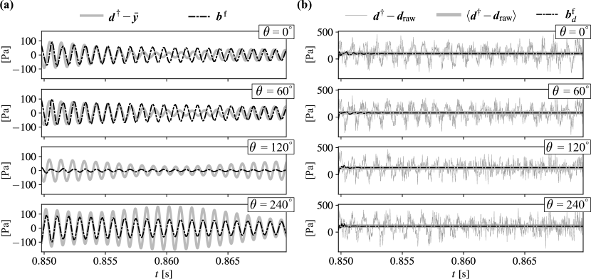
Figure 8: Bias-regularized r-EnKF. Comparison between the ESN inference of the biases and the (a) actual acoustic state (dashed black) and the presumed model bias from data (thick grey). (b) Measurement bias estimate (dashed black), difference between the raw and post-processed data (thin grey), and its time average, $\langle\cdot\rangle$ (thick grey). $\Phi=0.5125$.

On the other hand, the true value of the model bias is not known a priori, but it is presumed as ${\bm{\mathit{b}}}={\bm{\mathit{d}}}^{\dagger}-{\bm{\mathit{q}}}^{\dagger}$, where ${\bm{\mathit{q}}}^{\dagger}$ is the true model estimate, which is not known a priori. The digital twin improves the knowledge that we have on the model bias by correcting the presumed model bias.

To summarize, the r-EnKF generalizes to unseen scenarios and extrapolates correctly in time. Key to the robust performance is the inference of the biases in the model and measurements.

5.3 Physical parameters and comparison with the literature

We analyse the system’s physical parameters (§2.2 and equation (4)) for all the available equivalence ratios. We train an ESN for each equivalence ratio. The data assimilation parameters (assimilation window, frequency, ensemble size, etc.) are the same in all tests (D). We compare the low-order model parameters (i) inferred by the bias-unregularized EnKF, (ii) inferred by the bias-regularized r-EnKF, and (iii) obtained with the state-of-the-art Langevin regression by Indlekofer et al. (2022). The linear growth rate, $\nu$, and the heat source strength weighted by the symmetry intensity, $c_{2}\beta$ are shown in Figure 9; and the remaining parameters are shown in Figure 10. The specific values parameters are listed in E.

Figure 9: Comparison of the estimated values of the two stability parameters $c_{2}\beta$ (circles) and $\nu$ (triangles) after data assimilation, obtained with the bias-unregularized EnKF (black) and the r-EnKF with different bias regularization parameters (colour maps). Lighter colours indicate stronger regularization; larger marker sizes indicate more accurate solutions, i.e., smaller RMS errors; and the error bars represent the ensemble standard deviation. The dashed lines corresponds to the parameters identified by offline Langevin regression (Indlekofer et al., 2022).

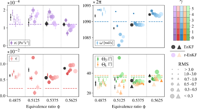
Figure 10: Same as Figure 9 for the remaining physical parameters.

First, the bias-regularized EnKF infers physical parameters with a small generalization error (the RMS errors are small, depicted with large markers). Large values of the bias regularization, i.e., $\gamma\gtrsim 1$, provide the most accurate set of parameters. This physically means that the low-order model is a qualitatively accurate model because the bias has a small norm (which corresponds to a large $\gamma$). The bias-unregularized EnKF is outperformed in all cases. (The case with $\Phi=0.4875$ is a stable configuration with a trivial fixed point, which is why the parameters have a larger RMS.) Second, we analyse the uncertainty of the parameters, which is shown by an error bar. The height of the error bar is the ensemble standard deviation. The linear growth rate, $\nu$, and the angular frequency, $\omega$, are inferred with small uncertainties. Physically, this means that the model predictions are markedly sensitive to small changes in the linear growth rate and angular frequency. The prediction’s sensitivity to the parameters change with the equivalence ratio. Physically, the large sensitivity of the linear growth rate (i.e., the system’s linear stability) to the operating condition is a characteristic feature of thermoacoustic instabilities, in particular in annular combustors, in which eigenvalues are degenerate (e.g., Magri et al., 2023). Third, there exists multiple combination of parameters that provide a similar accuracy. For example, in the case $\Phi=0.5125$, there are different combinations of $\Theta_{\beta},\epsilon,c_{2}\beta$, which yield a small RMS. Fourth, we compare the digital twin with the state-of-the-art methods based on offline Langevin regression of Indlekofer et al. (2022) (horizontal dashed lines in Figures 9, 10). The inferred parameters are physically meaningful because they lie within value ranges that are similar to the parameters of the literature. The digital twin simultaneously infers all the parameters in real time, which overcomes the limitations of Langevin regression, which needs to be performed on one parameter at a time and offline. The digital twin parameters are optimal because they are the minimizers of (28). The case $\Phi=0.5625$ shows the largest deviation between what the digital twin infers and the results of the offline identification method based on Langevin regression. The solution, which lives on a generalized Bloch sphere (Magri et al., 2023), is further analysed with the quaternion ansätz of Ghirardo and Bothien (2018). Figure 11 shows the acoustic state for $\Phi=0.5625$ from the raw data (panel b), the offline Langevin regression identification (panel c), and the proposed digital twin (panel d). The real-time digital twin infers a set of physical parameters, which correctly capture the physical state of the azimuthal acoustic mode. The nature angle has a bimodal distribution with $|\chi|<\pi/4$, which means that the thermoacoustic instability is a mixed mode. The Langevin regression also provides a bimodal distribution in $\chi$, however, it does not represent the changes in the anti-nodal line, i.e., $\vartheta$. (The parameters identified offline in Indlekofer et al. (2022) and in Figures 9 and 10 were tuned through least-square linear fitting versus $\Phi$. When tuned for a specific $\Phi$, the offline parameters lead to state statistics that more closely match the observables.)

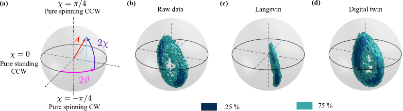
Figure 11: Acoustic state for $\Phi=0.5625$. (a) Bloch sphere for quaternion representation of the acoustic pressure $p(\theta,t)=A\cos{(\vartheta-\theta)}\cos{\chi}\cos{(\omega t+\varphi)}+A\sin{(\vartheta-\theta)}\sin{\chi}\sin{(\omega t+\varphi)}$, where $A$ is the slow-varying amplitude, i.e., the envelope of the acoustic pressure; $\varphi$, is the slow temporal phase drift, $\vartheta$ is the position of the anti-nodal line, and $\chi$ is the nature angle (Ghirardo and Bothien, 2018; Magri et al., 2023). (b) State from the raw data. (c) State probability deduced from Langevin regression methods (Indlekofer et al., 2022). (d) State predicted by the proposed real-time digital twin.

6 Conclusions

We develop a real-time digital twin of azimuthal thermoacoustics of a hydrogen-based combustor for uncovering the physical state from raw data, and predicting the nonlinear dynamics in time. We identify the four ingredients to design a robust real-time digital twin:

1. In a real-time context, we need to work with raw data as they come from sensors, therefore, we do not preprocess the data. The data we utilize is raw (the data contain both environmental and instrumental noise, and turbulent fluctuations) and sparse (the data are collected by four microphones).

2. A low-order model, which is deterministic, qualitatively accurate, computationally cheap, and physical.

3. An estimator of both the model bias, which originates from the modelling assumptions and approximation of a low-order model; and measurement bias, which originates from microphones recording the total pressure (which has a non-zero mean) instead of the acoustic pressure (which has zero mean).

4. A statistical data assimilation method that optimally combines the two sources of information on the system (i-ii) to improve the prediction on the physical states by updating the physical parameters every time that sensors’ data become available (on the fly, or real-time).

We propose a real-time data assimilation framework to infer the acoustic pressure, physical parameters, model biases and measurements biases simultaneously, which is the bias-regularized ensemble Kalman filter (r-EnKF). We find an analytical solution that minimizes the bias-regularized data assimilation cost function (28). We propose a reservoir computer (echo state network) and a training strategy to infer both the model bias a measurement bias, without making assumptions on their functional forms a priori. The real-time digital twin is applied to a laboratory hydrogen-based annular combustor for a variety of equivalence ratios. The data are treated as if they came from sensors on the fly, i.e., the pressure measurements are assimilated at a time step and then disregarded until the next pressure measurement becomes available. First, after assimilation of raw data (at 1707 Hz, i.e., approximately 0.6 data points per acoustic period), the model learns the correct physical state and optimal parameters. The real-time digital twin autonomously predicts azimuthal dynamics beyond the assimilation window, i.e., without seeing more data. This is in stark contrast with state-of-the-art methods based on the bias-unregularized methods, which do not perform well in the presence of model and measurement biases. Second, the digital twin uncovers the physical acoustic pressure from the raw data. Because the physical mechanisms are constrained in the low-order model, which originate from conservation laws, the digital twin acts as a physics-based filter, which removes aleatoric noise and turbulent fluctuations. Third, physically we find that azimuthal oscillations are governed by a time-varying parameter system, which generalizes existing models that have constant parameters, and capture only slow-varying variables. Fourth, we find that the key parameters that influence the dynamics are the linear growth rates, and the angular frequency. Further, the digital twin generalizes to equivalence ratios at which current modelling approaches are not accurate. This work opens new opportunities for real-time digital twinning of multi-physics problems. Current work is focused on exploring the role of sparsity in the data.

Declaration of interest

The authors report no conflict of interest.

Appendix A The ensemble Kalman filter

The classical (i.e., bias-unregularized) ensemble Kalman filter (EnKF) updates each ensemble member as Evensen (2003)

$${\bm{\mathit{\psi}}}_{j}^{\mathrm{a}} ={\bm{\mathit{\psi}}}_{j}^{\mathrm{f}}+\bm{\mathsf{K}}\left[{\bm{\mathit{d}}}_{j}-\bm{\mathsf{M}}{\bm{\mathit{\psi}}}_{j}^{\mathrm{f}}\right],\quad j=0,\dots,m-1,$$ (36)

$$\mathrm{with}\quad\bm{\mathsf{K}}=\bm{\mathsf{C}}_{\psi\psi}^{\mathrm{f}}\bm{\mathsf{M}}^{\mathrm{T}}\left(\bm{\mathsf{C}}_{dd}+\bm{\mathsf{M}}\bm{\mathsf{C}}_{\psi\psi}^{\mathrm{f}}\bm{\mathsf{M}}^{\mathrm{T}}\right)^{-1},$$

where $\bm{\mathsf{K}}$ is the Kalman gain matrix, and the superscripts ‘f’ and ‘a’ indicate ‘forecast’ and ‘analysis’, respectively. By evaluating the measurement operator products, we can write the EnKF update for the states and parameters of each ensemble member as

$$\begin{bmatrix}{\bm{\mathit{\phi}}}_{j}^{\mathrm{a}}\\[10.00002pt] {\bm{\mathit{\alpha}}}_{j}^{\mathrm{a}}\end{bmatrix} =\begin{bmatrix}{\bm{\mathit{\phi}}}_{j}^{\mathrm{f}}\\[10.00002pt] {\bm{\mathit{\alpha}}}_{j}^{\mathrm{f}}\end{bmatrix}+\underbrace{\begin{bmatrix}\bm{\mathsf{C}}_{\phi q}^{\mathrm{f}}\\[10.00002pt] \bm{\mathsf{C}}_{\alpha q}^{\mathrm{f}}\end{bmatrix}\left(\bm{\mathsf{C}}_{dd}+\bm{\mathsf{C}}_{qq}^{\mathrm{f}}\right)^{-1}}_{\mathrm{Kalman\,gain,\,\bm{\mathsf{K}}}}\overbrace{\left({\bm{\mathit{d}}}_{j}-{\bm{\mathit{q}}}_{j}^{\mathrm{f}}\right)}^{\mathrm{Innovation}}$$ (37)

As mentioned in §1, the EnKF is a bias-unregularized method. The estate and parameter update does not consider either the model bias or the measurement bias.

Appendix B Jacobian of the bias estimator

The Jacobian of the bias estimator is equivalent to the negative Jacobian of the ESN in open loop configuration, such that

$$\bm{\mathsf{J}}=\dfrac{\mathrm{d}\,{\bm{\mathit{b}}}^{\mathrm{f}}_{k+1}}{\mathrm{d}\,\bm{\mathsf{M}}\bar{{\bm{\mathit{\psi}}}}_{k}}=\dfrac{\mathrm{d}\,{\bm{\mathit{b}}}^{\mathrm{f}}_{k+1}}{\mathrm{d}\,\bar{{\bm{\mathit{i}}}}_{k}^{\mathrm{a}}}\dfrac{\mathrm{d}\,\bar{{\bm{\mathit{i}}}}_{k}^{\mathrm{a}}}{\mathrm{d}\,\bm{\mathsf{M}}\bar{{\bm{\mathit{\psi}}}}_{k}}=-\dfrac{\mathrm{d}\,{\bm{\mathit{b}}}^{\mathrm{f}}_{k+1}}{\mathrm{d}\,\bar{{\bm{\mathit{i}}}}_{k}}=-\bm{\mathsf{W}}_{\mathrm{out}}^{(1)}\left[\bm{\mathsf{T}}\odot\left(\sigma_{\mathrm{in}}\bm{\mathsf{W}}_{\mathrm{in}}^{(1)}\odot\bm{\mathsf{G}}\right)\right],$$ (38)

where $\bm{\mathsf{G}}=\left[{\bm{\mathit{g}}}~{}|\dots|~{}{\bm{\mathit{g}}}\right]^{\mathrm{T}}\in\mathbb{R}^{N_{q}\times N_{r}}$; ${\bm{\mathit{1}}}\in\mathbb{R}^{N_{r}}$ is a vector of ones; and $\bm{\mathsf{T}}=\left[{\bm{\mathit{T}}}~{}|\dots|~{}{\bm{\mathit{T}}}\right]\in\mathbb{R}^{N_{r}\times N_{q}}$ with

$${\bm{\mathit{T}}}={\bm{\mathit{1}}}-\tanh^{2}\left(\sigma_{\mathrm{in}}\bm{\mathsf{W}}_{\mathrm{in}}^{(1)}\left({\bm{\mathit{b}}}_{k}\odot{\bm{\mathit{g}}}\right)+\sigma_{\mathrm{in}}\delta_{\mathrm{r}}\bm{\mathsf{W}}_{\mathrm{in}}^{(2)}+\rho\bm{\mathsf{W}}{\bm{\mathit{r}}}_{k}\right).$$

For details on the derivation, the reader is referred to Nóvoa et al. (2024).

Appendix C Training the network

During training, the ESN is in open-loop configuration (Figure 3a). The inputs to the reservoir are the training dataset $\bm{\mathsf{U}}=\left[{\bm{\mathit{u}}}_{0}\,|\dots|\,{\bm{\mathit{u}}}_{N_{\mathrm{tr}}-1}\right]$, where each time component ${\bm{\mathit{u}}}_{k}=[{\bm{\mathit{b}}}_{\mathrm{u}}(t_{k});{{\bm{\mathit{i}}}}_{\mathrm{u}}(t_{k})]$ (the subscript ‘u’ indicates training data). Although we have information from the experimental data to train the network, the optimal parameters of the thermoacoustic system are unknown. Thus, we do not know a priori the model bias and measurement bias. Selecting an appropriate training dataset is essential to obtain a robust echo state network which can estimate the model bias and innovations. We create a set of $L$ guesses on the bias and innovations from a single realization of the experimental data. This means that the ESN is not trained with the ‘true’ bias.

The training data generation is summarized in Algorithm 1, and the procedure is as follows. First, we take measurements for a training time window $t_{\mathrm{train}}$ of acoustic pressure data $\bm{\mathsf{D}}_{\mathrm{u}}$, and we estimate $\bm{\mathsf{D}}^{\dagger}_{\mathrm{u}}$ by filtering the PSD of $\bm{\mathsf{D}}$ (see §2). Second, we draw $L$ sets of thermoacoustic parameters from uniform random distribution with lower and upper bounds ${\bm{\mathit{\alpha}}}^{0}(1-\sigma_{L})$ and ${\bm{\mathit{\alpha}}}^{0}(1+\sigma_{L})$, which are selected from an educated physical initial guess on the thermoacoustic model parameters. Then, we forecast the model (7) to statistically stationary conditions using the $L$ sets of parameters, and we take from each time series a sample of length $t_{\mathrm{train}}$, with this, we have the model estimates $\bm{\mathsf{Q}}_{\mathrm{u}}\in\mathbb{R}^{L\times N_{q}\times N_{\mathrm{train}}}$. Third, we correlate each $\bm{\mathsf{Q}}_{\mathrm{u},l}$ with the data by selecting the time lag $\varkappa\geq 0$ which minimizes their normalized root mean square error $(\mathrm{RMS})$ within the first 0.01 s (approximately 10 periods of the acoustic signal), i.e., for each $\bm{\mathsf{Q}}_{l}$, the time lag is $\varkappa_{l}=\{\varkappa\;s.t.\;\min{\mathrm{RMS}(\bm{\mathsf{Q}}_{\mathrm{u},l}(t-\varkappa),\bm{\mathsf{D}}(t))}\}$ with $t\in[0,0.01]$ s. Once the $L$ model estimates are aligned to the observations such that the RMS is minimized in the initial 10 periods of oscillation, we obtain the training model bias and innovations as

$$\bm{\mathsf{U}}_{l}=\left[\bm{\mathsf{B}}_{\mathrm{u},l};\bm{\mathsf{I}}_{\mathrm{u},l}\right]=\left[\bm{\mathsf{D}}^{\dagger}_{\mathrm{u}}-\bm{\mathsf{Q}}_{\mathrm{u},l};\bm{\mathsf{D}}_{\mathrm{u}}-\bm{\mathsf{Q}}_{\mathrm{u},l}\right],\quad\mathrm{for}\;l=0,\dots,L-1$$ (39)

If our initial guess in the parameters is well defined, the training bias dataset $\bm{\mathsf{B}}_{\mathrm{u}}$ have small norm. However, during assimilation the system can go through different states and parameter combinations, which may have a large norm model bias. Because the echo state network is only trained on the correlated signals, it may not be flexible to estimate the bias throughout DA Liang et al. (2023). Therefore, fourth, we apply data augmentation (Goodfellow et al., 2016) to increase the robustness of the ESN and improve the network adaptive in a real-time assimilation framework. We increase the training set by adding the bias and innovations resulting from mid-correlated signals to the training set. We select the mid-correlation time lag as the average between the best lag $\varkappa$ and the worst time lag. The total number of training time series in the proposed training method is $2L$. The training parameters used in this work are summarized in D.

Algorithm 1 Training dataset generation

1:${\bm{\mathsf{D}}_{\mathrm{u}}}\leftarrow$ Get observations(observation time = $t_{\mathrm{train}}$)

2:${\bm{\mathsf{D}}^{\dagger}_{\mathrm{u}}}\leftarrow$ Estimate truth($\bm{\mathsf{D}}_{\mathrm{u}}$)

3:${\bm{\mathsf{U}}}\leftarrow$ [ ]

4:for $l=0\;\mathbf{to}\;L-1$ do

5:     ${\bm{\mathit{\alpha}}}_{l}\leftarrow\mathcal{U}({\bm{\mathit{\alpha}}}^{0}(1-\sigma_{L}),{\bm{\mathit{\alpha}}}^{0}(1+\sigma_{L}))$

6:     $\bm{\mathsf{Q}}\leftarrow$ Forecast model(${\bm{\mathit{\alpha}}}_{l},t_{\mathrm{train}}$)

7:     $\bm{\mathsf{Q}}_{\mathrm{u},l}\leftarrow$ Correlate(${\bm{\mathsf{D}}_{\mathrm{u}}},\bm{\mathsf{Q}}$ ) $\triangleright$ Minimize RMS

8:     $\bm{\mathsf{U}}\leftarrow$ Append($[\bm{\mathsf{D}}_{\mathrm{u}}-\bm{\mathsf{Q}}_{\mathrm{u},l};\bm{\mathsf{D}}_{\mathrm{u}}^{\dagger}-\bm{\mathsf{Q}}_{\mathrm{u},l}]$ )

9:     $\bm{\mathsf{Q}}^{\mathrm{aug}}_{\mathrm{u},l}\leftarrow$ Mid-correlate(${\bm{\mathsf{D}}_{\mathrm{u}}},\bm{\mathsf{Q}}$ )$\triangleright$ Data augmentation

10:     $\bm{\mathsf{U}}\leftarrow$ Append($[\bm{\mathsf{D}}_{\mathrm{u}}-\bm{\mathsf{Q}}^{\mathrm{aug}}_{\mathrm{u},l};\bm{\mathsf{D}}_{\mathrm{u}}^{\dagger}-\bm{\mathsf{Q}}^{\mathrm{aug}}_{\mathrm{u},l}]$ )

Appendix D Simulations’ parameters

This appendix summarizes the parameters used for the data assimilation and for training the echo state network.

Table 1: Parameters used in the simulations.

Assimilation	$\Delta t_{\mathrm{d}}$	$35\Delta t$	s	$N_{q}$	4		$\sigma_{\mathrm{d}}$	0.1
	$\Delta t$	${51200}^{-1}$	s	$m$	20		$\omega$a	$[1090,1095]\cdot 2\pi$	Hz
	$\nu$a	$[-10,20]$	Hz	$c_{2}\beta$a	$[10,50]$	Hz	$\kappa$a	[1, 2]$\cdot 10^{-4}$	Hz
	$\Theta_{\beta}$a	$[0.5,0.7]$	rad	$\Theta_{\epsilon}$a	$[0.4,0.6]$	rad	$\epsilon$a	[5, 8] $\cdot 10^{-3}$
ESN training	$\Delta t_{\mathrm{ESN}}$	$5\Delta t$	s	$L$	50		$\lambda$b	$\{10^{-12},10^{-9}\}$
	$N_{r}$	50		Connectivity	3		$\sigma_{\mathrm{in}}$b	$[10^{-5},1]$
	$N_{\mathrm{wash}}$	10		$t_{\mathrm{train}}$	0.167	s	$\rho$b	$[0.5,1.0]$
	$N_{\mathrm{folds}}$	4		$t_{\mathrm{validate}}$	0.020	s
aIndicates that the parameters of the ensemble members are initialized within the given range.
bIndicates that the parameters are optimized in the given range.

Appendix E Inferred thermoacoustic parameters

Table 2 details the parameters shown in Figures 9-10. The reported parameters from the real-time digital twin (DT) are those with minimum RMS.

			Equivalence ratio
Param.	Units	Method
			$\Phi=0.4875$	$\Phi=0.5125$	$\Phi=0.5375$	$\Phi=0.5625$
		ref.	$-22.43$	$-6.58$	$9.26$	$25.11$
$\nu$	[Hz]	DT	$-18.48\pm 3.76$	$-4.84\pm 2.09$	$12.03\pm 3.21$	$25.13\pm 3.15$
		EnKF	$-1.31\pm 2.86$	$-32.09\pm 3.40$	$4.58\pm 2.57$	$24.42\pm 2.02$
		ref.	$17.65$	$24.11$	$30.57$	$37.02$
$c_{2}\beta$	[Hz]	DT	$30.64\pm 8.51$	$42.99\pm 6.86$	$46.84\pm 7.18$	$14.97\pm 3.97$
		EnKF	$27.77\pm 5.14$	$42.56\pm 9.64$	$49.55\pm 5.38$	$21.07\pm 1.76$
		ref.	$1.20$	$1.20$	$1.20$	$1.20$
$\kappa\cdot 10^{4}$	[Pa-2s-1]	DT	$1.55\pm 0.20$	$1.79\pm 0.19$	$1.62\pm 0.16$	$1.10\pm 0.12$
		EnKF	$1.59\pm 0.17$	$1.30\pm 0.21$	$1.23\pm 0.13$	$1.19\pm 0.09$
		ref.	$1090.00$	$1090.00$	$1090.00$	$1090.00$
$\omega/(2\pi)$	[rad s-1]	DT	$1092.36\pm 0.56$	$1085.29\pm 0.20$	$1089.05\pm 0.15$	$1092.32\pm 0.14$
		EnKF	$1091.78\pm 0.38$	$1087.92\pm 0.28$	$1088.98\pm 0.11$	$1092.19\pm 0.04$
		ref.	$2.30$	$2.30$	$2.30$	$2.30$
$\epsilon\cdot 10^{3}$	[ - ]	DT	$5.86\pm 0.57$	$2.71\pm 0.71$	$5.48\pm 0.55$	$7.74\pm 0.52$
		EnKF	$6.34\pm 0.38$	$8.13\pm 0.56$	$5.66\pm 0.41$	$8.63\pm 0.17$
		ref.	$36.10$	$36.10$	$36.10$	$36.10$
$\Theta_{\beta}$	[ ∘ ]	DT	$32.87\pm 1.83$	$31.93\pm 1.84$	$29.99\pm 0.65$	$35.50\pm 1.99$
		EnKF	$30.63\pm 1.35$	$34.07\pm 1.60$	$32.56\pm 0.89$	$31.64\pm 1.04$
		ref.	$37.82$	$37.82$	$37.82$	$37.82$
$\Theta_{\epsilon}$	[ ∘ ]	DT	$28.30\pm 2.13$	$21.72\pm 1.49$	$30.05\pm 0.62$	$28.87\pm 1.18$
		EnKF	$28.57\pm 1.44$	$26.03\pm 1.87$	$26.72\pm 0.67$	$37.84\pm 0.42$

Table 2: Thermoacoustic parameters inferred by the minimum-RMS solution (see Figure 9) of the digital twin (DT) and the bias-unregularized filter (EnKF) compared to the parameters identified by Indlekofer et al. (2022) (ref.).

References

- Aggarwal (2018) Charu C. Aggarwal. Neural networks and deep learning. Springer, 10, 2018.
- Aguilar Pérez et al. (2021) Jose G. Aguilar Pérez, James R. Dawson, Thierry Schuller, Daniel Durox, Kevin Prieur, and Sébastien Candel. Locking of azimuthal modes by breaking the symmetry in annular combustors. Combustion and Flame, 234:111639, 2021.
- Ahn et al. (2022) Byeonguk Ahn, Thomas Indlekofer, James R. Dawson, and Nicholas A. Worth. Heat release rate response of azimuthal thermoacoustic instabilities in a pressurized annular combustor with methane/hydrogen flames. Combustion and Flame, 244:112274, 2022.
- Bauerheim et al. (2014) Michael Bauerheim, Jean-François Parmentier, Pablo Salas, Franck Nicoud, and Thierry Poinsot. An analytical model for azimuthal thermoacoustic modes in an annular chamber fed by an annular plenum. Combustion and Flame, 161(5):1374–1389, 2014.
- Bauerheim et al. (2016) Michaël Bauerheim, Franck Nicoud, and Thierry Poinsot. Progress in analytical methods to predict and control azimuthal combustion instability modes in annular chambers. Physics of Fluids, 28(2), 2016.
- Bonavita and Laloyaux (2020) Massimo Bonavita and Patrick Laloyaux. Machine learning for model error inference and correction. Journal of Advances in Modeling Earth Systems, 12(12):e2020MS002232, 2020.
- Bothien et al. (2015) Mirko R. Bothien, Nicolas Noiray, and Bruno Schuermans. Analysis of azimuthal thermo-acoustic modes in annular gas turbine combustion chambers. Journal of Engineering for Gas Turbines and Power, 137(6):061505, 2015.
- Boujo et al. (2020) Edouard Boujo, Claire Bourquard, Yuan Xiong, and Nicolas Noiray. Processing time-series of randomly forced self-oscillators: the example of beer bottle whistling. Journal of Sound and Vibration, 464:114981, 2020.
- Bourgouin et al. (2013) Jean-Francois Bourgouin, Daniel Durox, Jonas P. Moeck, Thierry Schuller, and Sébastien Candel. Self-sustained instabilities in an annular combustor coupled by azimuthal and longitudinal acoustic modes. In Turbo Expo: Power for Land, Sea, and Air, volume 55119, page V01BT04A007. American Society of Mechanical Engineers, 2013.
- Brajard et al. (2020) Julien Brajard, Alberto Carrassi, Marc Bocquet, and Laurent Bertino. Combining data assimilation and machine learning to emulate a dynamical model from sparse and noisy observations: A case study with the Lorenz 96 model. Journal of computational science, 44:101171, 2020.
- Burgers et al. (1998) Gerrit Burgers, Peter Jan van Leeuwen, and Geir Evensen. Analysis scheme in the ensemble Kalman filter. Monthly weather review, 126(6):1719–1724, 1998.
- Callaham et al. (2021) Jared L. Callaham, J-C Loiseau, Georgios Rigas, and Steven L Brunton. Nonlinear stochastic modelling with langevin regression. Proceedings of the Royal Society A, 477(2250):20210092, 2021.
- Candel (2002) Sébastien Candel. Combustion dynamics and control: Progress and challenges. Proceedings of the combustion institute, 29(1):1–28, 2002.
- Candel et al. (2009) Sébastien Candel, Daniel Durox, Sébastien Ducruix, A-L Birbaud, Nicolas Noiray, and Thierry Schuller. Flame dynamics and combustion noise: progress and challenges. International Journal of Aeroacoustics, 8(1):1–56, 2009.
- Colburn et al. (2011) C. H. Colburn, J. B. Cessna, and T. R. Bewley. State estimation in wall-bounded flow systems. Part 3. The ensemble Kalman filter. Journal of Fluid Mechanics, 682:289–303, 2011.
- Culick (1988) Fred E. C. Culick. Combustion instabilities in liquid-fuelled propulsion systems. In AGARD Conference proceedings, volume 450, pages 1–73, 1988.
- Culick (2006) Fred E. C. Culick. Unsteady motions in combustion chambers for propulsion systems. North Atlantic Treaty Organization, RTO AGAR-Dograph AG-AVT-039, December 2006. doi: 10.14339/RTO-AG-AVT-039.
- da Silva and Colonius (2020) André F. C. da Silva and Tim Colonius. Flow state estimation in the presence of discretization errors. Journal of Fluid Mechanics, 890, 2020.
- Dee (2005) Dick P. Dee. Bias and data assimilation. Quarterly Journal of the Royal Meteorological Society: A journal of the atmospheric sciences, applied meteorology and physical oceanography, 131(613):3323–3343, 2005.
- Dee and da Silva (1998) Dick P. Dee and Arlindo M. da Silva. Data assimilation in the presence of forecast bias. Quarterly Journal of the Royal Meteorological Society, 124(545):269–295, 1998.
- Dee and Todling (2000) Dick P. Dee and Ricardo Todling. Data assimilation in the presence of forecast bias: The GEOS moisture analysis. Monthly Weather Review, 128(9):3268–3282, 2000.
- Donato et al. (2024) Laura Donato, Chiara Galletti, and Alessandro Parente. Self-updating digital twin of a hydrogen-powered furnace using data assimilation. Applied Thermal Engineering, 236:121431, 2024.
- Dowling and Morgans (2005) Ann P. Dowling and Aimee S. Morgans. Feedback control of combustion oscillations. Annual Review of Fluid Mechanics, 37(1):151–182, 2005. doi: 10.1146/annurev.fluid.36.050802.122038.
- Duran and Morgans (2015) Ignacio Duran and Aimee S. Morgans. On the reflection and transmission of circumferential waves through nozzles. Journal of Fluid Mechanics, 773:137–153, 2015.
- Durbin and Koopman (2012) James Durbin and Siem Jan Koopman. Time Series Analysis by State Space Methods. Oxford University Press, 05 2012. ISBN 9780199641178. doi: 10.1093/acprof:oso/9780199641178.001.0001. URL https://doi.org/10.1093/acprof:oso/9780199641178.001.0001.
- Evensen (2003) Geir Evensen. The ensemble Kalman filter: Theoretical formulation and practical implementation. Ocean dynamics, 53(4):343–367, 2003.
- Evensen (2009) Geir Evensen. Data assimilation: the ensemble Kalman filter. Springer Science & Business Media, 2009.
- Faure-Beaulieu and Noiray (2020) Abel Faure-Beaulieu and Nicolas Noiray. Symmetry breaking of azimuthal waves: Slow-flow dynamics on the Bloch sphere. Physical Review Fluids, 5(2):023201, 2020.
- Faure-Beaulieu et al. (2021a) Abel Faure-Beaulieu, Thomas Indlekofer, James R. Dawson, and Nicolas Noiray. Experiments and low-order modelling of intermittent transitions between clockwise and anticlockwise spinning thermoacoustic modes in annular combustors. Proceedings of the Combustion Institute, 38(4):5943–5951, 2021a.
- Faure-Beaulieu et al. (2021b) Abel Faure-Beaulieu, Thomas Indlekofer, James R. Dawson, and Nicolas Noiray. Imperfect symmetry of real annular combustors: beating thermoacoustic modes and heteroclinic orbits. Journal of Fluid Mechanics, 925:R1, 2021b.
- Friedland (1969) Bernard Friedland. Treatment of bias in recursive filtering. IEEE Transactions on Automatic Control, 14(4):359–367, 1969.
- Gao et al. (2017) Xinfeng Gao, Yijun Wang, Nathaniel Overton, Milija Zupanski, and Xuemin Tu. Data-assimilated computational fluid dynamics modeling of convection-diffusion-reaction problems. Journal of computational science, 21:38–59, 2017.
- Ghirardo and Bothien (2018) Giulio Ghirardo and Mirko R. Bothien. Quaternion structure of azimuthal instabilities. Physical Review Fluids, 3(11):113202, 2018.
- Ghirardo and Juniper (2013) Giulio Ghirardo and Matthew P. Juniper. Azimuthal instabilities in annular combustors: standing and spinning modes. Proceedings of the Royal Society A: Mathematical, Physical and Engineering Sciences, 469(2157):20130232, 2013.
- Goodfellow et al. (2016) Ian Goodfellow, Yoshua Bengio, and Aaron Courville. Deep learning. MIT press, 2016.
- Grigoryeva and Ortega (2018) Lyudmila Grigoryeva and Juan-Pablo Ortega. Echo state networks are universal. Neural Networks, 108:495–508, 2018. ISSN 0893-6080. doi: 10.1016/j.neunet.2018.08.025.
- Haimberger (2007) Leopold Haimberger. Homogenization of radiosonde temperature time series using innovation statistics. Journal of Climate, 20(7):1377–1403, 2007.
- Hansen et al. (2024) James J. Hansen, Davy Brouzet, and Matthias Ihme. A normal-score ensemble Kalman filter for 1D shock waves. In AIAA SCITECH 2024 Forum, page 1022, 2024.
- Huhn and Magri (2020) Francisco Huhn and Luca Magri. Learning ergodic averages in chaotic systems. In International Conference on Computational Science, pages 124–132. Springer, 2020.
- Humbert et al. (2023a) Sylvain C. Humbert, Jonas P. Moeck, Christian Oliver Paschereit, and Alessandro Orchini. Symmetry-breaking in thermoacoustics: Theory and experimental validation on an annular system with electroacoustic feedback. Journal of Sound and Vibration, 548:117376, 2023a.
- Humbert et al. (2023b) Sylvain C. Humbert, Alessandro Orchini, Christian Oliver Paschereit, and Nicolas Noiray. Symmetry breaking in an experimental annular combustor model with deterministic electroacoustic feedback and stochastic forcing. Journal of Engineering for Gas Turbines and Power, 145(3):031021, 2023b.
- Ignagni (1990) Mario B. Ignagni. Separate bias Kalman estimator with bias state noise. IEEE Transactions on Automatic Control, 35(3):338–341, 1990.
- Illingworth and Morgans (2010) Simon J. Illingworth and Aimee S. Morgans. Adaptive feedback control of combustion instability in annular combustors. Combustion science and technology, 182(2):143–164, 2010.
- Indlekofer et al. (2021) Thomas Indlekofer, Abel Faure-Beaulieu, Nicolas Noiray, and James R. Dawson. The effect of dynamic operating conditions on the thermoacoustic response of hydrogen rich flames in an annular combustor. Combustion and Flame, 223:284–294, 2021.
- Indlekofer et al. (2022) Thomas Indlekofer, Abel Faure-Beaulieu, James R. Dawson, and Nicolas Noiray. Spontaneous and explicit symmetry breaking of thermoacoustic eigenmodes in imperfect annular geometries. Journal of Fluid Mechanics, 944:A15, 2022.
- Jaeger and Haas (2004) Herbert Jaeger and Harald Haas. Harnessing nonlinearity: Predicting chaotic systems and saving energy in wireless communication. Science, 304(5667):78–80, 2004.
- Juniper and Sujith (2018) Matthew P. Juniper and Raman I. Sujith. Sensitivity and nonlinearity of thermoacoustic oscillations. Annual Review of Fluid Mechanics, 50(1):661–689, January 2018. doi: 10.1146/annurev-fluid-122316-045125.
- Kalman (1960) Rudolph Emil Kalman. A new approach to linear filtering and prediction problems. Journal of basic Engineering, 82(1):35–45, 1960.
- Kolouri et al. (2013) Soheil Kolouri, Mahmood R Azimi-Sadjadi, and Astrid Ziemann. Acoustic tomography of the atmosphere using unscented kalman filter. IEEE transactions on geoscience and remote sensing, 52(4):2159–2171, 2013.
- Krebs et al. (2002) Werner Krebs, Patrick Flohr, Bernd Prade, and Stefan Hoffmann. Thermoacoustic stability chart for high-intensity gas turbine combustion systems. Combustion science and technology, 174(7):99–128, 2002.
- Labahn et al. (2019) Jeffrey W. Labahn, Hao Wu, Bruno Coriton, Jonathan H. Frank, and Matthias Ihme. Data assimilation using high-speed measurements and LES to examine local extinction events in turbulent flames. Proceedings of the Combustion Institute, 37(2):2259–2266, 2019.
- Laera et al. (2017) Davide Laera, Thierry Schuller, Kevin Prieur, Daniel Durox, Sergio M. Camporeale, and Sébastien Candel. Flame describing function analysis of spinning and standing modes in an annular combustor and comparison with experiments. Combustion and Flame, 184:136–152, 2017.
- Laloyaux et al. (2020) Patrick Laloyaux, Massimo Bonavita, Mohamed Dahoui, J. Farnan, Sean Healy, E. Hólm, and S. T. K. Lang. Towards an unbiased stratospheric analysis. Quarterly Journal of the Royal Meteorological Society, 146(730):2392–2409, 2020.
- Liang et al. (2023) Jianyu Liang, Koji Terasaki, and Takemasa Miyoshi. A machine learning approach to the observation operator for satellite radiance data assimilation. Journal of the Meteorological Society of Japan. Ser. II, 101(1):79–95, 2023.
- Lieuwen (2003) Tim C Lieuwen. Statistical characteristics of pressure oscillations in a premixed combustor. Journal of Sound and Vibration, 260(1):3–17, 2003.
- Lieuwen (2012) Tim C. Lieuwen. Unsteady combustor physics. Cambridge University Press, Cambridge, 2012. ISBN 978-1-139-05996-1. doi: 10.1017/CBO9781139059961.
- Lieuwen et al. (2001) Tim C. Lieuwen, H. Torres, C. Johnson, and B. T. Zinn. A mechanism of combustion instability in lean premixed gas turbine combustors. Journal of Engineering for Gas Turbines and Power, 123(1), 2001. doi: 10.1115/1.1339002.
- Lukoševičius (2012) Mantas Lukoševičius. A practical guide to applying echo state networks. In Neural networks: Tricks of the trade, pages 659–686. Springer, 2012.
- Magri and Doan (2020) Luca Magri and Nguyen Anh Khoa Doan. Physics-informed data-driven prediction of turbulent reacting flows with Lyapunov analysis and sequential data assimilation. In Data Analysis for Direct Numerical Simulations of Turbulent Combustion, pages 177–196. Springer, 2020.
- Magri et al. (2016a) Luca Magri, Michael Bauerheim, and Matthew P. Juniper. Stability analysis of thermo-acoustic nonlinear eigenproblems in annular combustors. part i. sensitivity. Journal of Computational Physics, 325:395–410, 2016a.
- Magri et al. (2016b) Luca Magri, Michael Bauerheim, Franck Nicoud, and Matthew P. Juniper. Stability analysis of thermo-acoustic nonlinear eigenproblems in annular combustors. part ii. uncertainty quantification. Journal of Computational Physics, 325:411–421, 2016b.
- Magri et al. (2020) Luca Magri, Matthew P. Juniper, and Jonas P. Moeck. Sensitivity of the Rayleigh criterion in thermoacoustics. Journal of Fluid Mechanics, 882:R1, 2020.
- Magri et al. (2023) Luca Magri, Peter J. Schmid, and Jonas P. Moeck. Linear flow analysis inspired by mathematical methods from quantum mechanics. Annual Review of Fluid Mechanics, 55:541–574, 2023.
- Majda and Harlim (2012) Andrew J. Majda and John Harlim. Filtering complex turbulent systems. Cambridge University Press, 2012.
- Mazur et al. (2019) Marek Mazur, Håkon T. Nygård, James R. Dawson, and Nicholas A. Worth. Characteristics of self-excited spinning azimuthal modes in an annular combustor with turbulent premixed bluff-body flames. Proceedings of the Combustion Institute, 37(4):5129–5136, 2019.
- Mazur et al. (2021) Marek Mazur, Yi Hao Kwah, Thomas Indlekofer, James R. Dawson, and Nicholas A. Worth. Self-excited longitudinal and azimuthal modes in a pressurised annular combustor. Proceedings of the Combustion Institute, 38(4):5997–6004, 2021.
- Mensah et al. (2019) Georg A. Mensah, Luca Magri, Alessandro Orchini, and Jonas P. Moeck. Effects of asymmetry on thermoacoustic modes in annular combustors: a higher-order perturbation study. Journal of Engineering for Gas Turbines and Power, 141(4):041030, 2019.
- Moeck et al. (2010) Jonas P. Moeck, Markus Paul, and Christian Oliver Paschereit. Thermoacoustic instabilities in an annular Rijke tube. In Turbo Expo: Power for Land, Sea, and Air, volume 43970, pages 1219–1232, 2010.
- Morgans and Stow (2007) Aimee S. Morgans and Simon R. Stow. Model-based control of combustion instabilities in annular combustors. Combustion and flame, 150(4):380–399, 2007.
- Murthy et al. (2019) Sandeep R. Murthy, Taraneh Sayadi, Vincent Le Chenadec, Peter J. Schmid, and Daniel J. Bodony. Analysis of degenerate mechanisms triggering finite-amplitude thermo-acoustic oscillations in annular combustors. Journal of Fluid Mechanics, 881:384–419, 2019.
- Noiray (2017) Nicolas Noiray. Linear growth rate estimation from dynamics and statistics of acoustic signal envelope in turbulent combustors. Journal of Engineering for Gas Turbines and Power, 139(4), 2017.
- Noiray and Schuermans (2013a) Nicolas Noiray and Bruno Schuermans. Deterministic quantities characterizing noise driven Hopf bifurcations in gas turbine combustors. International Journal of Non-Linear Mechanics, 50:152–163, 2013a.
- Noiray and Schuermans (2013b) Nicolas Noiray and Bruno Schuermans. On the dynamic nature of azimuthal thermoacoustic modes in annular gas turbine combustion chambers. Proceedings of the Royal Society A: Mathematical, Physical and Engineering Sciences, 469(2151):20120535, 2013b.
- Noiray et al. (2011) Nicolas Noiray, Mirko Bothien, and Bruno Schuermans. Investigation of azimuthal staging concepts in annular gas turbines. Combustion Theory and Modelling, 15(5):585–606, 2011.
- Nóvoa et al. (2024) Andrea Nóvoa, Alberto Racca, and Luca Magri. Inferring unknown unknowns: regularized bias-aware ensemble kalman filter. Computer Methods in Applied Mechanics and Engineering, 418:116502, 2024.
- Nóvoa and Magri (2022) Andrea Nóvoa and Luca Magri. Real-time thermoacoustic data assimilation. Journal of Fluid Mechanics, 948:A35, 2022. doi: 10.1017/jfm.2022.653.
- Orchini et al. (2020) Alessandro Orchini, Luca Magri, Camilo F. Silva, Georg A. Mensah, and Jonas P. Moeck. Degenerate perturbation theory in thermoacoustics: high-order sensitivities and exceptional points. Journal of Fluid Mechanics, 903:A37, 2020.
- O’Connor et al. (2013) Jacqueline O’Connor, Nicholas A. Worth, and James R. Dawson. Flame and flow dynamics of a self-excited, standing wave circumferential instability in a model annular gas turbine combustor. In Turbo Expo: Power for Land, Sea, and Air, volume 55119, page V01BT04A063. American Society of Mechanical Engineers, 2013.
- Paschereit et al. (1998) Christian O. Paschereit, Ephraim Gutmark, and Wolfgang Weisenstein. Structure and control of thermoacoustic instabilities in a gas-turbine combustor. Combustion Science and Technology, 138(1-6):213–232, 1998.
- Poinsot (2017) Thierry Poinsot. Prediction and control of combustion instabilities in real engines. Proceedings of the Combustion Institute, 36(1):1–28, 2017.
- Racca and Magri (2021) Alberto Racca and Luca Magri. Robust optimization and validation of echo state networks for learning chaotic dynamics. Neural Networks, 142:252–268, 2021.
- Rayleigh (1878) Lord Rayleigh. The explanation of certain acoustical phenomena. Nature, 18:319–321, July 1878. doi: 10.1038/018319a0.
- Roy et al. (2021) Amitesh Roy, Samarjeet Singh, Asalatha Nair, Swetaprovo Chaudhuri, and Raman I. Sujith. Flame dynamics during intermittency and secondary bifurcation to longitudinal thermoacoustic instability in a swirl-stabilized annular combustor. Proceedings of the Combustion Institute, 38(4):6221–6230, 2021.
- Schuermans et al. (2006) Bruno Schuermans, Christian Oliver Paschereit, and Peter Monkewitz. Non-linear combustion instabilities in annular gas-turbine combustors. In 44th AIAA aerospace sciences meeting and exhibit, page 549, 2006.
- Silva (2023) Camilo F. Silva. Intrinsic thermoacoustic instabilities. Progress in Energy and Combustion Science, 95:101065, 2023.
- Tarantola (2005) Albert Tarantola. Inverse Problem Theory and Methods for Model Parameter Estimation. Society for Industrial and Applied Mathematics, 2005. ISBN 9780898715729.
- Traverso and Magri (2019) Tullio Traverso and Luca Magri. Data Assimilation in a Nonlinear Time-Delayed Dynamical System with Lagrangian Optimization. Computational Science – ICCS 2019, page 156–168, 2019. ISSN 1611-3349.
- Wang et al. (2021) Peng Wang, Chuangxin He, Zhiwen Deng, and Yingzheng Liu. Data assimilation of flow-acoustic resonance. The Journal of the Acoustical Society of America, 149(6):4134–4148, 2021.
- Wolf et al. (2012) Pierre Wolf, Gabriel Staffelbach, Laurent YM Gicquel, Jens-Dominik Müller, and Thierry Poinsot. Acoustic and large eddy simulation studies of azimuthal modes in annular combustion chambers. Combustion and Flame, 159(11):3398–3413, 2012.
- Worth and Dawson (2013a) Nicholas A. Worth and James R. Dawson. Modal dynamics of self-excited azimuthal instabilities in an annular combustion chamber. Combustion and Flame, 160(11):2476–2489, 2013a.
- Worth and Dawson (2013b) Nicholas A. Worth and James R. Dawson. Self-excited circumferential instabilities in a model annular gas turbine combustor: Global flame dynamics. Proceedings of the Combustion Institute, 34(2):3127–3134, 2013b.
- Yang et al. (2019) Dong Yang, Davide Laera, and Aimee S. Morgans. A systematic study of nonlinear coupling of thermoacoustic modes in annular combustors. Journal of Sound and Vibration, 456:137–161, 2019. ISSN 0022-460X. doi: 10.1016/j.jsv.2019.04.025.
- Yu et al. (2019a) Hans Yu, Matthew P. Juniper, Thomas Jaravel, Matthias Ihme, and Luca Magri. Data assimilation and optimal calibration in nonlinear models of flame dynamics. ASME Turbo Expo GT2019-92052, 2019a.
- Yu et al. (2019b) Hans Yu, Matthew P. Juniper, and Luca Magri. Combined state and parameter estimation in level-set methods. Journal of Computational Physics, 399:108950, 2019b.