Certification of Speaker Recognition Models to Additive Perturbations

Abstract

Speaker recognition technology is applied in various tasks ranging from personal virtual assistants to secure access systems. However, the robustness of these systems against adversarial attacks, particularly to additive perturbations, remains a significant challenge. In this paper, we pioneer applying robustness certification techniques to speaker recognition, originally developed for the image domain. In our work, we cover this gap by transferring and improving randomized smoothing certification techniques against norm-bounded additive perturbations for classification and few-shot learning tasks to speaker recognition. We demonstrate the effectiveness of these methods on VoxCeleb 1 and 2 datasets for several models. We expect this work to improve voice-biometry robustness, establish a new certification benchmark, and accelerate research of certification methods in the audio domain.

1550

1 Introduction

This work addresses the issues of robustness and privacy in deep learning voice biometry models [36, 38]. Although deep learning models excel in various applications, they are unreliable and susceptible to specific perturbations. These perturbations may be imperceptible to humans but can dramatically affect the models’ performance [37]. For instance, minor adjustments in the brightness or contrast of X-ray images could lead to a false-negative diagnosis. Researchers have developed various adversarial attacks and empirical defenses, leading to a certification paradigm that provides provable guarantees on model behavior under constrained perturbations [22, 9]. However, speech algorithms have received less attention compared to ones from image processing. Given the escalating levels of speech fraud due to advancements in adversarial models and deep fake technologies [32], significant security risks could arise in biometric systems or even in creating personalized scams on social networks. Thus, this article focuses on the certification of automatic speaker recognition models, a topic not yet thoroughly examined in the literature.

Speaker recognition models [12, 4, 40] often use spectrograms (typically Mel spectrograms) or raw-waveform frontends and may be designed for several tasks. Firstly, identification classifies who is speaking in a given audio. Secondly, verification determines whether two audios belong to the same speaker. Finally, diarization segments a given audio into distinct speech parts corresponding to different speakers. These biometry models train to convert speech into vector representations such that utterances from the same speaker yield closely spaced vectors, while those from different speakers produce widely spaced vectors. Several training approaches exist for the encoder that maps audio $x$ to embeddings for subsequent classification. One method involves ordinary classification with a fixed set of training speakers, where variations of cross-entropy loss initially developed for face biometry [26] enhance the expressiveness and separation of embeddings. Another method employs metric learning using triplet [17] or contrastive [39] loss. During inference, cosine similarity or distance metrics help identify the closest embedding among the reference speakers’ embeddings (enrollment vectors) to the embedding of the given audio.

Our work explores the certified robustness of speaker recognition models against any additive perturbation constrained by the $l_{2}$ norm value. Such perturbations can result from various adversarial attacks, whether targeted or untargeted, and white-box or black-box scenarios where the attacker may know the model’s architecture, parameters, and gradients or may only have input and output access.

Our contributions are summarized as follows:

• We introduce a novel randomized smoothing-based approach to certify few-shot embedding models against additive, norm-bounded perturbations.

• We derive robustness certificates and theoretically demonstrate their advantages over those obtained using existing competitors’ methods. Our theoretical claims are supported by experimental results on the VoxCeleb datasets with the use of several well-known speaker recognition models.

• We highlight the issue of certified robustness in speaker recognition models and establish a new benchmark for certification in this area.

2 Methods

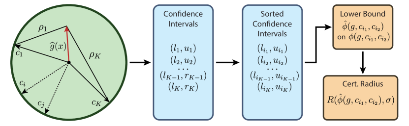
Figure 1: The scheme illustrating the proposed Algorithm 1. Given a sample $x$, base model $f$, set of prototypes $\{c_{1},\dots,c_{K}\}$ (enrollment vectors), variance $\sigma^{2}$, confidence level $\alpha$ and number of samples $N$ and maximum number of samples $T$, Algorithm computes the lower bound $R(\hat{\phi}(g,c_{i_{1}},c_{i_{2}}))$ on the certified radius $R({\phi}(g,c_{i_{1}},c_{i_{2}}))$ from the Theorem 1.

In this section, we define the problem statement, provide an overview of the techniques used, and describe the proposed method for certifying speaker embedding models against norm-bounded additive perturbations. This method is based on the randomized smoothing framework within a few-shot learning setting for speaker recognition [9, 34].

2.1 Speaker Recognition Problem as a Few-Shot Problem

Consider $f:[-1,1]^{n}\to\mathbb{R}^{d}$ as the base model that maps input audios to normalized embeddings, where $\|f(\cdot)\|_{2}=1$. After training the embedding model, an enrollment (or prototype) database is constructed for the further use. The enrollment vector for a speaker is a reference embedding used during the inference or production stage to calculate similarity with the embedding of the provided new audio. The speaker’s enrollment vector is usually created as a mean or weighted sum of embeddings that are created from several speaker’s audios. During the enrollment stage, we are given a set $S=\{(x_{1},y_{1}),\dots,(x_{l},y_{l})\}$ of audios $x_{i}\in[-1,1]^{n}$, each assigned to a corresponding speaker $y_{i}\in[1,\dots,K]$. It’s important to note that this database might consist of entirely new speakers unseen during training or a combination of seen and unseen speakers, depending on the application.

Suppose $S_{k}={(x_{i},y_{i})\in S:y_{i}=k}$ is the subset of $S$ containing audios belonging to class $k$, forming the normalized class enrollment embedding

$$c_{k}=\frac{1}{|S_{k}|}\sum_{x\in S_{k}}f(x),\ ~{}\|c_{k}\|_{2}=1,$$ (1)

during the model’s enrollment stage. Then, during inference, a new incoming sample $x$ is assigned to the class $c$ with the closest prototype:

$$c=c(x)=\operatorname*{argmin}_{k\in[1,\dots,K]}\|f(x)-c_{k}\|_{2}.$$ (2)

2.2 Randomized Smoothing

In a common setting, randomized smoothing is an averaging of the base model prediction over the input perturbed by additive Gaussian noise.

Namely, given the model $f:\mathbb{R}^{n}\to[0,1]^{K}$ and the smoothing distribution $\mathcal{N}(0,\sigma^{2}I)$ the smoothed model takes the form

$$g(x)=\mathbb{E}_{\varepsilon\sim\mathcal{N}(0,\sigma^{2}I)}f(x+\varepsilon).$$ (3)

here $g(x)$ is the vector of class probabilities with $K$ components. As it is shown in [9], when the model from Eq. (3) is confident in predicting the correct class $c$ for the object $x$,

$$g(x)_{c}=p_{A}\geq p_{B}=\max_{i\neq c}g(x)_{i}$$ (4)

then it is robust in $l_{2}-$ball around $x$ of radius

$$R=\frac{\sigma}{2}\left(\Phi^{-1}(p_{A})-\Phi^{-1}(p_{B})\right),$$ (5)

where $\Phi^{-1}(\cdot)$ is the inverse of the standard Gaussian CDF, meaning

$$\operatorname*{argmin}_{k\in[1,\dots K]}\|g(x)-c_{k}\|_{2}=\operatorname*{argmin}_{k\in[1,\dots K]}\|g(x+\delta)-c_{k}\|_{2}$$ (6)

for all perturbations $\delta:\|\delta\|_{2}<R.$

2.3 1-Lipschitz Randomized Smoothing for Vector Functions

In this section, we describe our method and formulate the robustness guarantee against $l_{2}$-norm bounded adversarial attacks.

Given the base model $f:[0,1]^{n}\to[0,1]^{d}$ that maps input to normalized embeddings, the associated smoothed model $g:[0,1]^{n}\to[0,1]^{d}$ is defined as

$$g(x)=\mathbb{E}_{\varepsilon\sim\mathcal{N}(0,\sigma^{2}I)}f(x+\varepsilon).$$ (7)

Here $g(x)$ is $d-$dimensional embedding. Suppose that the class prototypes $c_{1},\dots,c_{K}$ from Eq. (1) are known and input image $x$ is correctly assigned to class $c$ represented by prototype $c_{i_{1}}$ and $c_{i_{2}}$ is the second closest to $g(x)$ prototype. If we introduce scalar mapping $\phi:\mathbb{R}^{d}\to[0,1]$ in the form

$$\phi=\phi(g,c_{i_{1}},c_{i_{2}})=\frac{\langle g(x),c_{i_{1}}-c_{i_{2}}\rangle}{2\|c_{i_{1}}-c_{i_{2}}\|_{2}}+\frac{1}{2},$$ (8)

then the following robustness guarantee holds.

Theorem 1 (Main result).

For all additive perturbations $\delta:\|\delta\|_{2}\leq R(\phi,\sigma)=\sigma\Phi^{-1}(\phi)$

$$\operatorname*{argmin}_{k\in[1,\dots K]}\|g(x)-c_{k}\|_{2}=\operatorname*{argmin}_{k\in[1,\dots K]}\|g(x+\delta)-c_{k}\|_{2},$$ (9)

where $R(\phi,\sigma)$ is called certified radius of $g$ at $x.$

The detailed proof is provided in the Appendix.

3 Implementation Details

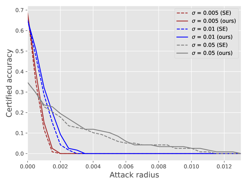
(a) Dependency on $\sigma$

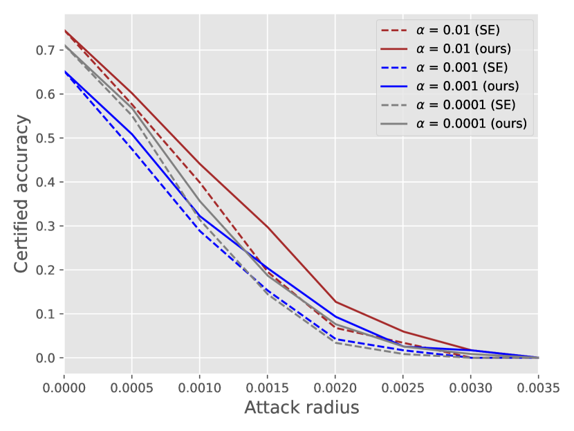
(b) Dependency on $\alpha$

(c) Dependency on $N_{\text{max}}$

Figure 2: Pyannote model. Few-shot setting. Dependency of certified accuracy on $\sigma$, $\alpha$, and $N_{\text{max}}$. Comparison of SE [30] and our approaches.

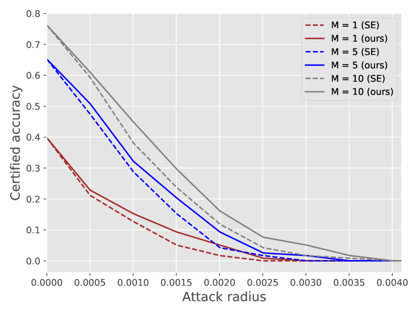
(a) Dependency on $M$

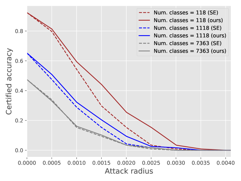
(b) Dependency on number of speakers.

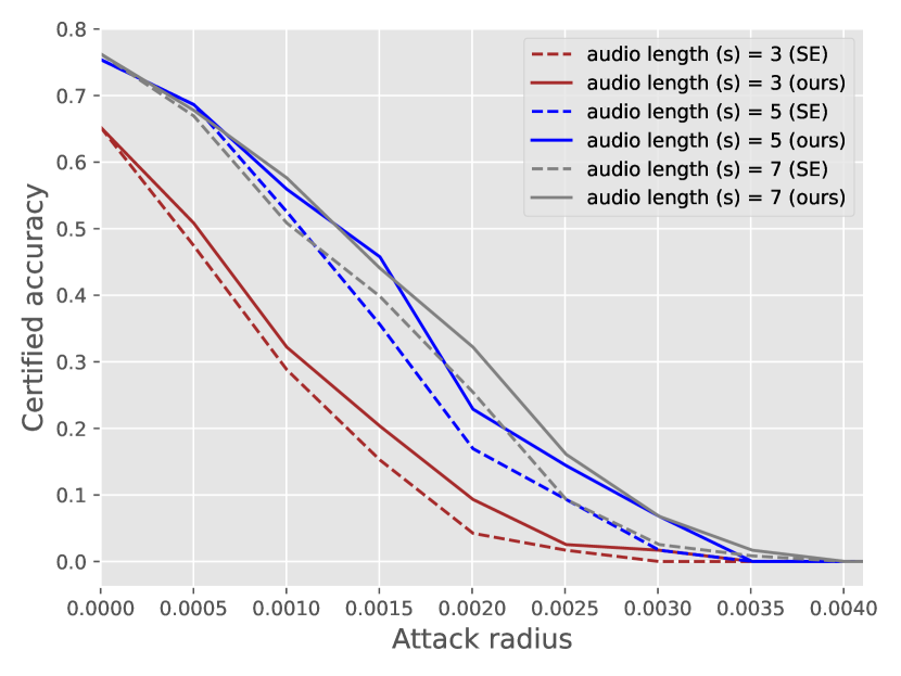
(c) Dependency on the audio length $n$.

Figure 3: Pyannote model. Few-shot setting. Dependency of certified accuracy on $M$, audio length $n$, and the number of presented in enrollment set classes.

(a) Dependency on $\sigma$

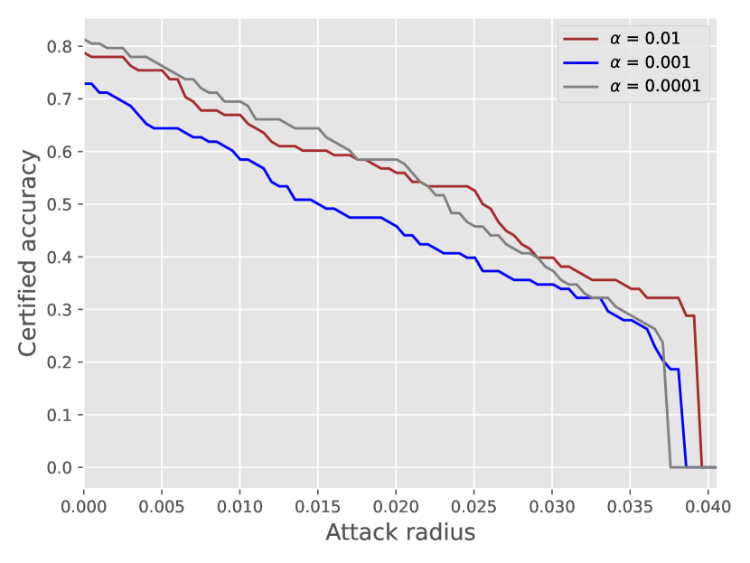
(b) Dependency on $\alpha$

(c) Dependency on $N_{\text{max}}$

Figure 4: Pyannote model. Classification setting. Dependency of certified accuracy on $\sigma$, $\alpha$, and $N_{\text{max}}$.

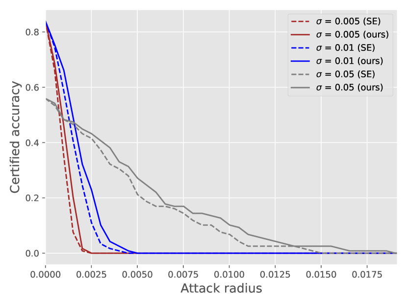
(a) Dependency on $\sigma$

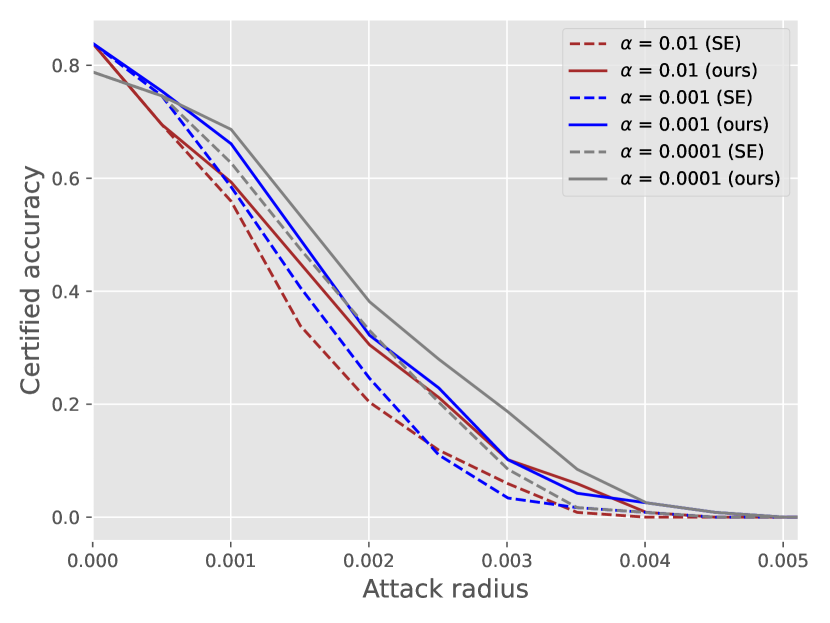
(b) Dependency on $\alpha$

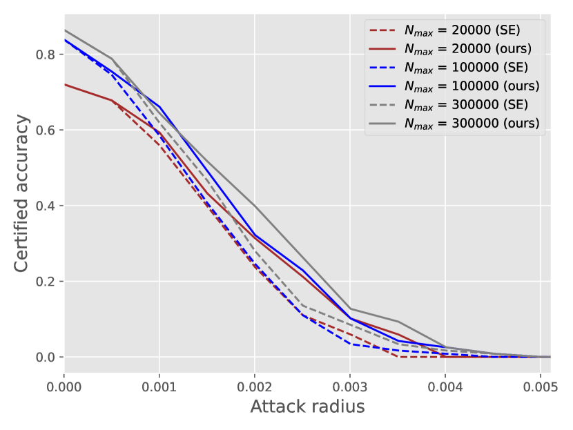
(c) Dependency on $N_{\text{max}}$

Figure 5: ECAPA-TDNN model. Few-shot setting. Dependency of certified accuracy on $\sigma$, $\alpha$, and $N_{\text{max}}$. Comparison of SE and our approaches.

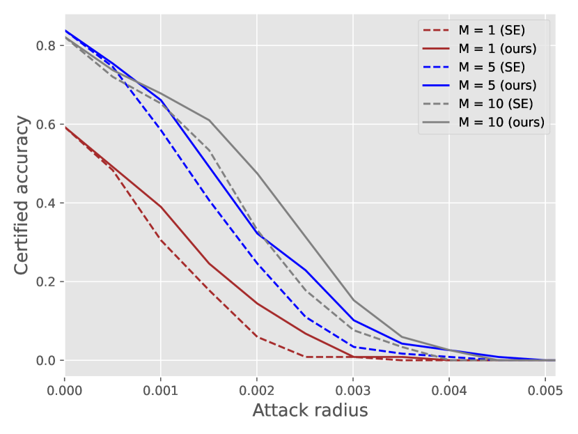
(a) Dependency on $M$

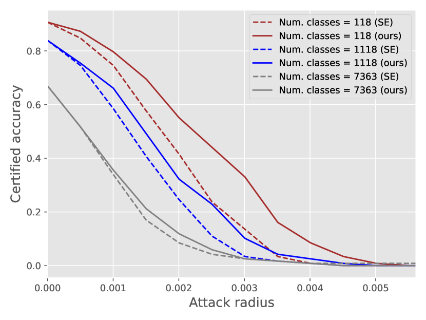
(b) Dependency on number of speakers.

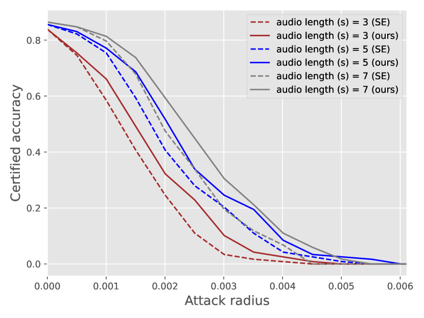
(c) Dependency on the audio length $n$.

Figure 6: ECAPA-TDNN model. Few-shot setting. Dependency of certified accuracy on $M$ and number of presented in enrollment set classes.

(a) Dependency on $\sigma$

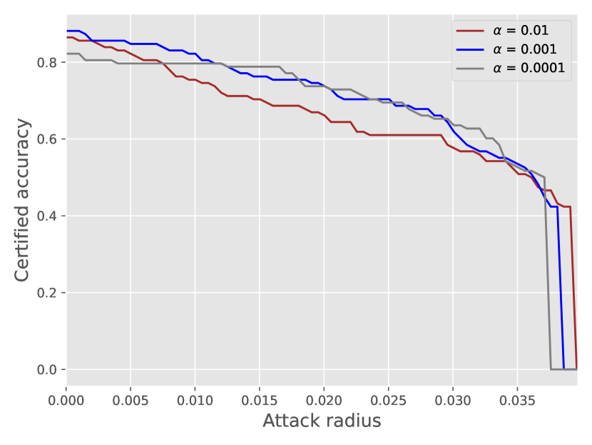
(b) Dependency on $\alpha$

(c) Dependency on $N_{\text{max}}$

Figure 7: ECAPA-TDNN model. Classification setting. Dependency of certified accuracy on $\sigma$, $\alpha$, and $N_{\text{max}}$.

In this section, we describe the numerical implementation of our method.

3.1 Sample Mean Instead of Expectation

It is noteworthy that the prediction of the smoothed model from Eq. (7) is an expected value of the random variable that is the function of the base classifier, hence, it is impossible to evaluate it exactly in case of nontrivial $f.$ Consequently, it is impossible to evaluate the mapping $\phi$ from Eq. (8). A conventional way to deal with this problem is to replace the smoothed model with its unbiased estimation – sample mean computed over $N$ samples, namely

$$\hat{g}(x)=\frac{1}{N}\sum_{i=1}^{N}f(x+\varepsilon_{i}),$$ (10)

where $\varepsilon_{i}$ are realizations of a normally distributed random variable. However, it is also impossible to accurately determine which two prototypes $c_{i}$ and $c_{j}$ are the closest to the true value of the smoothed classifier from Eq. (7).

We solve the aforementioned issues in the following manner.

1. First of all, we compute interval estimations of the distances between $g(x)$ and all the prototypes using Hoeffding inequality [18]. It is done to determine the two closest prototypes with a sufficient level of confidence.

2. Secondly, given the two closest prototypes, we compute the lower bound $\hat{\phi}$ of an interval estimate of $\phi$ from Eq. (8).

3. Finally, than $\hat{\phi}$ is computed, the value $R(\hat{\phi},\sigma)$ from Theorem 1 is treated as the certified radius of $g$ at $x.$

1:function CertRadius($f,x,N,T,\sigma,\alpha$)

2:     $\operatorname{isFinished}\leftarrow\operatorname{False}$

3:     $N_{0}\leftarrow N$

4:     while $\operatorname{not}\operatorname{isFinished}$ or $N\leq T$ do

5:         $\varepsilon_{1},\dots,\varepsilon_{N}\sim\mathcal{N}(0,\sigma^{2}I)$

6:         $\varepsilon_{N+1},\dots,\varepsilon_{2N}\sim\mathcal{N}(0,\sigma^{2}I)$

7:         $\hat{g}_{1}(x)=\frac{1}{N}\sum_{j=1}^{N}f(x+\varepsilon_{j})$

8:         $\hat{g}_{2}(x)=\frac{1}{N}\sum_{j=1}^{N}f(x+\varepsilon_{N+j})$

9:         for $i\in\{1,\dots,K\}$ do

10:              $v^{1}_{i}=\hat{g}_{1}(x)-c_{i}$

11:              $v^{2}_{i}=\hat{g}_{2}(x)-c_{i}$

12:              $(l_{i},u_{i})\leftarrow\textsc{HoeffdingCI}(v^{1}_{i},v^{2}_{i},\alpha)$ $\triangleright$ Computation of two-sided confidence interval using Hoeffding inequality, namely $(l_{i},u_{i}):\mathbb{P}\left(\|{g}(x)-c_{i}\|_{2}\in(l_{i},u_{i})\right)\geq 1-\alpha$          

13:         $i_{1}\leftarrow\operatorname*{argmin}\{l_{1},\dots,l_{K}\}$

14:         $i_{2}\leftarrow\operatorname*{argmin}\{l_{1},\dots,l_{K}\setminus l_{i_{1}}\}$

15:         $i_{q}\leftarrow\operatorname*{argmin}\{l_{1},\dots,l_{K}\setminus\{l_{i_{1}},l_{i_{2}}\}\}$

16:         if $u_{i_{1}}<l_{i_{2}}\wedge u_{i_{2}}<l_{i_{q}}$ then

17:              $\operatorname{isFinished}\leftarrow\operatorname{True}$

18:              $\hat{g}(x)=\frac{\hat{g}_{1}(x)+\hat{g}_{2}(x)}{2}$

19:              $\tilde{\phi}\leftarrow\frac{\langle\hat{g}(x),c_{i_{1}}-c_{i_{2}}\rangle}{2\|c_{i_{1}}-c_{i_{2}}\|_{2}}+\frac{1}{2}$

20:              $\hat{\phi}\leftarrow\textsc{HoeffdingLowerBound}(\tilde{\phi},\alpha)$

21:              $R\leftarrow\sigma\Phi^{-1}(\hat{\phi})$

22:              return R

23:         else

24:              if $2N>T$ then

25:                  return Abstain

26:              else

27:                  $N\leftarrow N+N_{0}$                             

Algorithm 1 Computation of certified radius.

3.2 Hoeffding Confidence Interval and Error Probability

Hoeffding inequality [18] bounds the probability of a large deviation of a sample mean from the population mean, namely

$$\mathbb{P}(|\overline{X}-\mathbb{E}(X)|\geq t)\leq 2\exp\left(-\frac{2t^{2}N^{2}}{\sum_{i=1}^{N}(b_{i}-a_{i})^{2}}\right),$$ (11)

where $\overline{X}=\frac{1}{N}\sum_{i=1}^{N}X_{i},$ and $X_{i}$ are i.i.d. random variables such that $\mathbb{P}(X_{i}\in(a_{i},b_{i})=1).$

In this section, we describe the procedures of estimating the distances between the output of the smoothed model and class prototypes, estimating the value of $\phi$ from Theorem 1 and the error probability of each procedure.

3.2.1 Distances to the Class Prototypes.

An estimation of distance between the smoothed embedding $g(x)$ from Eq. (7) and the class prototype $c_{i}$ from Eq. (1) may be derived from an estimation of the dot product $\langle\hat{g}_{1}(x)-c_{i},\hat{g}_{2}(x)-c_{i}\rangle,$ where

$$\hat{g}_{1}(x)=\frac{1}{N}\sum_{i=1}^{N}f(x+\varepsilon_{i})\ \text{and}$$ (12)

$$\hat{g}_{2}(x)=\frac{1}{N}\sum_{j=1}^{N}f(x+\varepsilon_{j})$$ (13)

are two independent unbiased estimates of $g(x).$ Once computed, confidence interval $(l^{2}_{i},u^{2}_{i})$ for the expression $\langle\hat{g}_{1}(x)-c_{i},\hat{g}_{2}(x)-c_{i}\rangle$ implies confidence interval $(l_{i},u_{i})$ of interest. The work of [30] provides a detailed derivation of the confidence interval.

3.2.2 Estimation of $\phi$.

Hoeffding inequality is also used to compute confidence intervals for the value $\phi$ from Theorem 1. Namely, given

$$\tilde{\phi}-\frac{1}{2}=\frac{\left\langle\frac{\hat{g}_{1}(x)+\hat{g}_{2}(x)}{2},c_{i_{1}}-c_{i_{2}}\right\rangle}{2\|c_{i_{1}}-c_{i_{2}}\|_{2}}.$$ (14)

as an estimation of $\phi-\frac{1}{2}$ over $2N$ samples $\xi_{j}$ in the form

$$\xi_{j}=\frac{\langle f(x+\varepsilon_{j}),c_{i_{1}}-c_{i_{2}}\rangle}{2\|c_{i_{1}}-c_{i_{2}}\|_{2}}.$$ (15)

such that $\xi_{j}\in[-\frac{1}{2},\frac{1}{2}],$ we compute lower bound $\hat{\phi}-\frac{1}{2}$ of $\phi-\frac{1}{2}$ in the form

$$\hat{\phi}-\frac{1}{2}=\tilde{\phi}-\frac{1}{2}-\sqrt{\frac{\ln{\frac{2}{\alpha}}}{4N}}.$$ (16)

Note that $\alpha$ in Eq. (16) is the upper bound for the error probability. In other words,

$$\mathbb{P}(\phi<\hat{\phi})<\alpha.$$ (17)

All the procedures are combined in the numerical pipeline which is presented in the Algorithm 1.

3.2.3 Error Probability of the Algorithm 1.

Since the procedure in Algorithm 1 is not deterministic (as it depends on the computation of confidence intervals), it is important to estimate its failure probability. First of all, note that if all the distances between smoothed embedding and class prototypes are located within corresponding confidence intervals, the two closest prototypes are determined correctly. In contrast, if at least one of distances

$$\|g(x)-c_{1}\|_{2},\dots,\|g(x)-c_{K}\|_{2}$$ (18)

is not within the corresponding interval, it is impossible to guarantee that two closest prototypes are correctly determined, thus, all the respective Hoeffding inequalities have to hold. It happens with the probability $p_{1}=(1-\alpha)^{K},$ where $K$ is the number of classes. Secondly, note that the lower confidence bound for $\phi$ from Theorem 1 is correct with probability $p_{2}=(1-\alpha).$

Thereby, the probability of the correct output of Algorithm 1 is $p_{1}p_{2}=(1-\alpha)^{K+1}$ what leads to the error probability $q=1-(1-\alpha)^{K+1}.$

4 Experiments

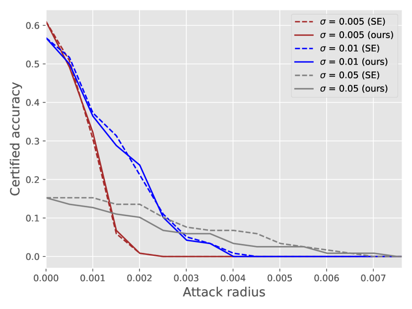
(a) Wespeaker

(b) CAM++

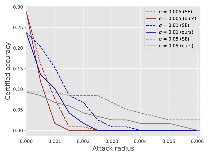
(c) ERes2Net

Figure 8: Few-shot setting. Dependency of certified accuracy on $\sigma$. Comparison of SE and our approaches for several models. $N_{\text{max}}=5000$.

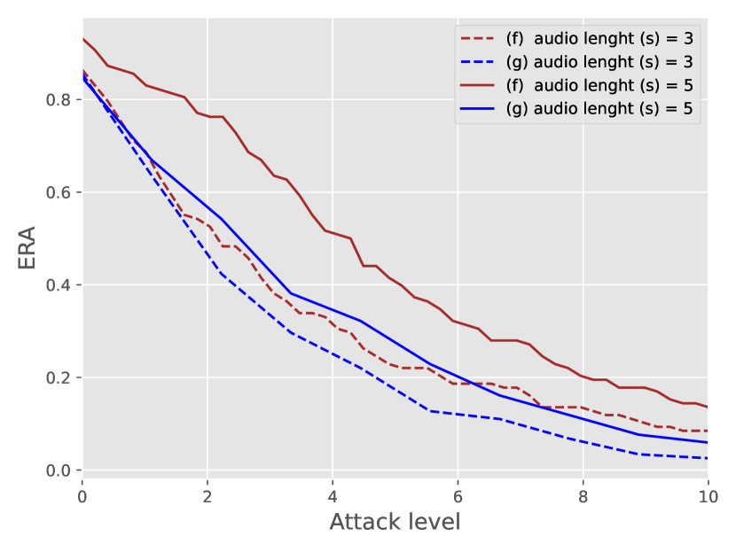
(a) Gaussian noise.

(b) PGD

Figure 9: Pyannote model. Comparison of empirical robust accuracy (ERA) of base $f$ and smooth $g$ speaker recognition (embedding) models against additive perturbation: Gaussian noise and PGD adversarial attack.

4.1 Datasets

For our experiments, we selected the VoxCeleb1 [28] and VoxCeleb2 [7] datasets, commonly used for speaker recognition and speaker verification tasks. These datasets provide links and timestamps to YouTube videos, allowing for potential computer vision applications, though our focus is solely on the audio component. VoxCeleb1 includes 1211 development and 40 test speakers, with a total of over 150000 utterances spanning more than 350 hours. VoxCeleb2, in contrast, contains 5994 development and 118 test speakers, totaling approximately 2400 hours across about 1.1 million utterances. These datasets are multilingual, featuring speakers from over 140 different nationalities and encompassing a wide range of accents and ages. We assessed our methods on 118 VoxCeleb2 speakers, varying the number of enrolled speakers from those corresponding to the test speakers only (118) to the entire development portion of both datasets combined with the test speakers (7323).

4.2 Evaluation Protocol

We evaluate the methods in several settings. Experiments are conducted using various backbone embedding models: ECAPA-TDNN [12] from the Speechbrain framework [33]; the Pyannote framework [4], which focuses on speaker diarization and utilizes the raw-waveform frontend SincNet; and ResNet-based models such as Cam++ [41] and ERes2Net [5] from the Wespeaker framework [40]. These models transform speech into vector representations of dimensions 192, 256, or 512. We applied training with Gaussian noise as data augmentation to enhance the empirical resistance to norm-bounded attacks for ECAPA-TDNN, but this did not yield significant improvements as the models were already trained with adequate noise levels.

For the certification procedure from the Algorithm 1, the default parameters of the system are the following: standard deviation of additive noise used for smoothing is set to $\sigma=10^{-2}$, maximum number of samples $T=N_{\text{max}}$ is set to be $10^{5}$, the confidence level $\alpha$ is set to be $\alpha=10^{-3}$, default number of enrolled classes is $1118$, default number of random support audios per class (speaker) that are used to compute the class prototype (enrollment vector of the class) is set to $M=5$, and length of given audios is set to be 3s with sampling rate 16000 Hz is $n=48000$.

We compared our approach to the work of [30], where authors propose the method called Smoothed Embeddings (SE), to certify prototypical networks. The certified radius $R^{SE}(x)$ produced by SE has the form

$$R^{SE}(x)=\sqrt{\frac{\pi\sigma^{2}}{2}}\frac{\|c_{i_{2}}-g(x)\|_{2}^{2}-\|c_{i_{1}}-g(x)\|_{2}^{2}}{2\|c_{i_{1}}-c_{i_{2}}\|^{2}_{2}}.$$ (19)

in our notation. In contrast to our work, they perform a geometrical analysis of Lipschitz properties of the smoothed model, whereas we study the properties of the scalar mapping from the embedding space.

We also provide results from ordinary randomized smoothing [9, 34] for the classification task 5 using the same default set of parameters. Since an exact estimation of $g(x)$ is impossible, a similar sample-mean is utilized but with the Clopper-Pearson [8] test for the lower confidence bound of $\hat{p}_{A}$. In a nutshell, this is a Binomial proportion confidence interval of top class v.s. the rest. Thus, for certification it is required that during the sampling the correct class is predicted in more than half of cases: $\hat{p}_{A}>\frac{1}{2}$.

4.3 Results and Discussion

For the evaluation, we sampled a random subset $\hat{S}$ consisting of several audios from each of the 118 test speakers. For each method, we report certified accuracy (CA) on the subset $\hat{S}$. Certified accuracy represents the proportion of correctly classified samples from $\hat{S}$ for which the smoothed model has a certified radius exceeding the given attack magnitude. Specifically, given the classification rule

$$c(x)=\operatorname*{argmin}_{k\in\{1,\dots,K\}}\|g(x)-c_{k}\|_{2}.$$ (20)

and the norm of perturbation $\varepsilon,$ the certified accuracy is computed as follows:

$$CA(\hat{S},\varepsilon)=\frac{|(x,y)\in\hat{S}:R(x)>\varepsilon\ \wedge\ c(x)=y|}{|\hat{S}|}.$$ (21)

In Eq. (21), $R(x)$ denotes the certified radius of the smoothed model at $x.$

The computational time required for certifying one sample with default parameters is approximately 30 seconds for the Pyannote model, 120 seconds for ECAPA-TDNN, and approximately 4300 seconds for Wespeaker models, which do not support batch processing during inference.

The results are illustrated in Figures 2-8. We compared randomized smoothing, the SE method, and our approach under varying certification parameters. The results indicate that our method significantly outperforms the SE approach but performs worse than randomized smoothing in a classification context.

In figure 9, we also demonstrate the empirical robust accuracy (ERA), a fraction of correctly classified audios perturbed with noise less or equal to the threshold level. The presented ERA of predictions of $g$ on corrupted with projected gradient descent (PGD) attack is much larger than the certified accuracy of every method. Nonetheless, as it is only one particular attack on a finite set of perturbations, it does not necessarily convey the worst result, as there exist stronger attacks, and the worst-case ERA might be closer to CA. Additionally, the certification condition was checked adaptively and continued sampling could yield better results due to more accurate unbiased estimations and narrower confidence intervals.

It can be noticed from the figures that in some cases certified accuracy increases with an increase in the length of the audio. This means that the improvement in the quality of the embedding outperforms the negative influence of increased norm (actually, there is a trade-off 3(c)). Namely certification condition does not depend on audio length (depends on embeddings and prototypes) and provides a certified radius: maximum $l_{2}$ perturbation the prediction of smoothed models maintains the same. This level is the same for the input $x\in\mathbb{R}^{n}$. Thus, the relative distortion of the audio will be different for $n=48000$ and $n=80000$.

5 Limitations

It is important to mention that the current certification results are loose. There is a magnitude gap between certified and empirical accuracy, which is an upper bound for CA. Fine-tuning of models with additive Gaussian noise augmentations to make them more empirically and, consequently, certified robust to perturbations did not help, since the pre-trained ECAPA-TDNN model was already trained with the proper augmentations. For the Pyannote model, we did not manage to accomplish the fine-tuning as the model is trained in a speaker diarization setting. For other models, especially for ERes2Net, we will try to do fine-tuning in future work with noise augmentations and probably with adversarial training.

In our work, certification is limited to additive perturbations. However, it is feasible to extend this to multiplicative and semantic transformations [27, 23] by applying different mappings and smoothing distributions. Nonetheless, these methods are not capable of certifying speaker encoder models against the contemporary and rapidly evolving threats posed by deep-fakes [44] in the current landscape.

Certification is achievable against $l_{2}$ norm-bounded attacks, not against $l_{\infty}$. However, it seems to be unsolvable according to [16]. One can estimate the upper bound on certified radii $R_{\infty}$ as $\frac{R_{2}}{\sqrt{n}}$ which is a rather small bound.

Additionally, the certification result depends on the length of the audio sample, however, 3-5 seconds of audio might be sufficient for voice-biometry applications, especially in streaming services.

6 Related Work

6.1 Speaker Recognition

Recently, speaker recognition [36, 38, 12, 41, 40] has made significant progress. The x-vector system, which is based on Time Delay Neural Network (TDNN)  technology, has been particularly influential and further applied and developed in many other models. This system uses one-dimensional convolution to pick up important time-related features in speech. For example, building on the x-vector model, ECAPA-TDNN uses techniques that allow the model to consider a wider range of time-related information, combining information from several filter banks in one first intermediate state and recursively from several previous states for the next hidden state. Later, a densely connected time delay neural network (D-TDNN) was presented, that reduces the number of parameters needed. Additionally, the Context-Aware Masking (CAM) module, a type of pooling, was combined with D-TDNN, and the model CAM++ improves the performance in terms of verification metrics (EER, MinDCF) and inference time.

6.2 Adversarial Attacks

It has long been known [37, 14] that deep learning models are vulnerable to small additive perturbations of input. In recent years, many approaches have been proposed to generate adversarial examples, for example, [3, 46, 42]. These methods expose different conceptual vulnerabilities of models: some generate attacks using information about the model’s gradient, while others deploy separate networks to produce malicious input. Moreover, adversarial examples can be transferred across models [19], which limits the application of neural networks in various practical scenarios. This vulnerability poses significant risks in contexts such as biomedical image segmentation [2], industrial face recognition [21] and detection [20], self-driving car systems [11], and speaker recognition systems [47, 24]. Additionally, speaker anonymization systems (SAS) aim to conceal identity features while preserving other information (text, emotions) from speech utterances, thereby enhancing the privacy of voice data, for instance, with virtual assistants. Current approaches are based on digital signal processing, feature extraction of the speaker, audio re-generation, and the generation of additive perturbations [10], which can be considered as a form of adversarial attack.

6.3 Empirical and Certified Defenses

To mitigate the effects of attacks, numerous defensive approaches have recently been proposed [22, 13]. Among these, adversarial training [14, 1] is arguably the best technique to enhance the robustness of models in practice. The method is straightforward – during training, each batch of data is augmented with adversarial 337 examples generated by a specific method. Consequently, the model becomes more resistant to the type of attack used during the training process. However, the model may easily become overfitted to the provided attacks and unable to defend against new types of adversarial perturbations. Additionally, adversarial training is time-consuming and often leads to decreased plain accuracy due to the robustness-accuracy trade-off. Despite this, several prominent fast adversarial training approaches exist. Nonetheless, ordinary augmentations with Gaussian noise or semantic transformation are the simplest, cheapest, and still prominent approaches to increase the empirical robustness of models. In addition, regularization techniques (e.g., consistency loss) are also applied.

Another research direction is the development of methods that provide provable certificates on the model’s prediction under certain transformations. Mainly, approaches are based on SMT [31] and MILP [6] solvers, on interval [15] and polyhedra [25] relaxation, on analysis of Lipschitz continuity [34], curvatures of the network [35].

Randomized smoothing [9, 34] forms the basis for many certification approaches, offering defenses against both norm-bounded [45] and semantic perturbations [23, 27]. This simple, effective, and scalable technique is also used for certifying automatic speaker recognition systems [29]. Additionally, self-supervised methods [43] are employed to provide empirical guarantees in speaker recognition.

7 Conclusion

In this work, we presented a new approach to certify speaker embedding models that map input audios to normalized embeddings against norm-bounded additive perturbations. We introduce a scalar mapping from the embedding space and derive theoretical robustness guarantees based on its Lipschitz properties. We have experimentally evaluated our approach against several concurrent methods. Although our approach yields worse results compared to the standard randomized smoothing approach in a classification setting, it outperforms the method described in [30] in the few-shot setting.

In summary, we expect this work to highlight the issue of the certified robustness in biometric systems, particularly in voice biometry, to improve AI safety and to establish a new certification benchmark. Future developments in this topic might be devoted to the improvement of certified guarantees and the development of certification against other types of attacks, including non-analytical ones such as deep-fakes.

Appendix A Appendix

A.1 Proof of the Theorem

In this section, we provide the proof of Theorem 1.

Theorem 1 (Restated).

Let $g$ be the model from Eq. (7) and $c_{1},\dots,c_{K}$ be the class prototypes from Eq. (1). Suppose that image $x$ is correctly assigned to class $c$ represented by prototype $c_{i_{1}}$ and $c_{i_{2}}$ is the second closest to $g(x)$ prototype. Then for all additive perturbations $\delta:\|\delta\|_{2}\leq R(\phi,\sigma)=\sigma\Phi^{-1}(\phi),$

$$\arg\min_{k\in[1,\dots K]}\|g(x)-c_{k}\|_{2}=\arg\min_{k\in[1,\dots K]}\|g(x+\delta)-c_{k}\|_{2},$$ (22)

where $\phi=\phi(x)=\frac{\langle g(x),c_{i_{1}}-c_{i_{2}}\rangle}{2\|c_{i_{1}}-c_{i_{2}}\|_{2}}+\frac{1}{2}.$

Proof.

For simplicity, let $\sigma=1.$ Consider the function $\psi(x)=\langle 2g(x),c_{i_{1}}-c_{i_{2}}\rangle$ with the gradient

$$\nabla_{x}\psi(x)=\langle 2\nabla_{x}g(x),c_{i_{1}}-c_{i_{2}}\rangle,$$ (23)

$$\nabla_{x}\psi(x)=2\langle\int_{\mathbb{R}^{n}}f(x+\varepsilon)\varepsilon\rho(\varepsilon)d\varepsilon,c_{i_{1}}-c_{i_{2}}\rangle=\int_{\mathbb{R}^{n}}r(\varepsilon)\varepsilon\rho(\varepsilon)d\varepsilon,$$ (24)

where $\rho(\varepsilon)=\frac{1}{(2\pi)^{n/2}}\exp\left(-\frac{\|\varepsilon\|^{2}_{2}}{2}\right)$ and $r(\varepsilon)=2\langle f(x+\varepsilon),c_{i_{1}}-c_{i_{2}}\rangle$. Note that $r(\varepsilon)\in\left[-2\|c_{i_{1}}-c_{i_{2}}\|_{2},2\|c_{i_{1}}-c_{i_{2}}\|_{2}\right]$ and

$$\int_{\mathbb{R}^{n}}r(\varepsilon)\rho(\varepsilon)d\varepsilon=2\langle g(x),c_{i_{1}}-c_{i_{2}}\rangle=\psi(x).$$

Let us introduce $\hat{r}(\varepsilon)=\frac{r(\varepsilon)}{4\|c_{i_{1}}-c_{i_{2}}\|_{2}}+\frac{1}{2}$. Note that $\hat{r}(\varepsilon)\in[0,1]$ and $\int_{\mathbb{R}^{n}}\hat{r}(\varepsilon)\rho(\varepsilon)d\varepsilon=\phi(x).$ The expression of gradient from Eq. (23) takes the form

$$\nabla_{x}\psi(x)=\int_{\mathbb{R}^{n}}\big{[}4\|c_{i_{1}}-c_{i_{2}}\|_{2}\hat{r}(\varepsilon)-2\|c_{i_{1}}-c_{i_{2}}\|\big{]}\varepsilon\rho(\varepsilon)d\varepsilon=4\|c_{i_{1}}-c_{i_{2}}\|_{2}\int_{\mathbb{R}^{n}}\hat{r}(\varepsilon)\varepsilon\rho(\varepsilon)d\varepsilon.$$ (25)

To compute $\sup_{x}\left\|\nabla_{x}\psi(x)\right\|_{2},$ we need to find

$$\sup_{v:\|v\|_{2}=1}\mathbb{E}_{\varepsilon\sim\mathcal{N}(0,I)}\langle\hat{r}(\varepsilon)\varepsilon,v\rangle$$

$$\text{subject to}\ \mathbb{E}_{\varepsilon\sim\mathcal{N}(0,I)}\hat{r}(\varepsilon)=\phi(x).$$

According to [34],

$$\sup_{x}\left\|\nabla_{x}\psi(x)\right\|_{2}=\sup_{v:\|v\|_{2}=1}\langle\nabla_{x}\psi(x),v\rangle=\frac{4\|c_{i_{1}}-c_{i_{2}}\|_{2}}{\sqrt{2\pi}}\exp\left[-\frac{1}{2}\left(\Phi^{-1}(\phi(x))\right)^{2}\right]=z(\psi(x)),$$ (26)

where $\Phi^{-1}$ in the inverse of standard Gaussian CDF. Let’s introduce the function $\xi=\xi(\psi(x)):\mathbb{R}^{n}\to\mathbb{R}^{1}$ such that

$$\|\nabla_{x}\xi(\psi(x))\|\leq\left|\frac{d\xi}{d\psi}\right|\left\|\nabla_{x}\psi(x)\right\|(x)\equiv 1$$ (27)

and such that $\xi(\psi(x))$ is monotonically increasing, and, thus $\left|\frac{d\xi}{d\psi}\right|=\frac{d\xi}{d\psi}.$

$$\frac{d}{dx}\operatorname{erfc}^{-1}(x)=-\frac{1}{2}\sqrt{\pi}e^{\left[\operatorname{erfc}^{-1}(x)\right]^{2}}$$ (28)

Note that the function

$$\xi(\psi(x))=\int\frac{d\psi(x)}{z(\psi(x))}=\frac{\sqrt{2\pi}}{4\|c_{i_{1}}-c_{i_{2}}\|_{2}}\int\exp\left[\frac{1}{2}\left(\Phi^{-1}(\phi)\right)^{2}\right]d\psi(x)=\Phi^{-1}(\phi(x))$$ (29)

satisfies Eq. (27).
Thus, function $\xi(\psi(x))=\Phi^{-1}(\phi(x))$ has Lipschitz constant $L\leq 1,$ or, equivalently, $\forall\delta$

$$\|\xi(\psi(x))-\xi(\psi(x+\delta))\|_{2}\leq\|\delta\|_{2}.$$ (30)

Since $x$ is correctly classified by $g$, $\psi(x)>0$ and $\phi(x)>\frac{1}{2}.$ Note that all the perturbations $\tilde{\delta}$ such that $\psi(x+\tilde{\delta})=0$ have norm not less than $\Phi^{-1}(\phi(x))$, since

$$\|\xi(\psi(x))-\xi(\psi(x+\tilde{\delta}))\|_{2}\leq\|\tilde{\delta}\|_{2}\Rightarrow\xi(\psi(x))=\Phi^{-1}(\phi(x))\leq\|\tilde{\delta}\|.$$ (31)

Consequently, all perturbations $\hat{\delta}$ such that $\psi(x+\hat{\delta})\leq 0$ have norm not less than $\Phi^{-1}(\phi(x))$ since $\psi(x)$ is continuous.

Finally, that means that for all perturbations $\delta:\|\delta\|_{2}<\xi(\psi(x))=\Phi^{-1}(\phi(x))\Rightarrow\psi(x)>0,$ what finalizes the proof. The proof for the cases when $\sigma\neq 1$ is analogous.

∎

A.2 Additional Experiments

In this section, we present the results of other experiments.

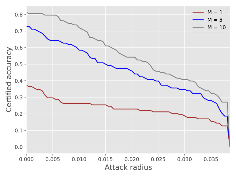
(a) Dependency on $M$

(b) Dependency on number of speakers.

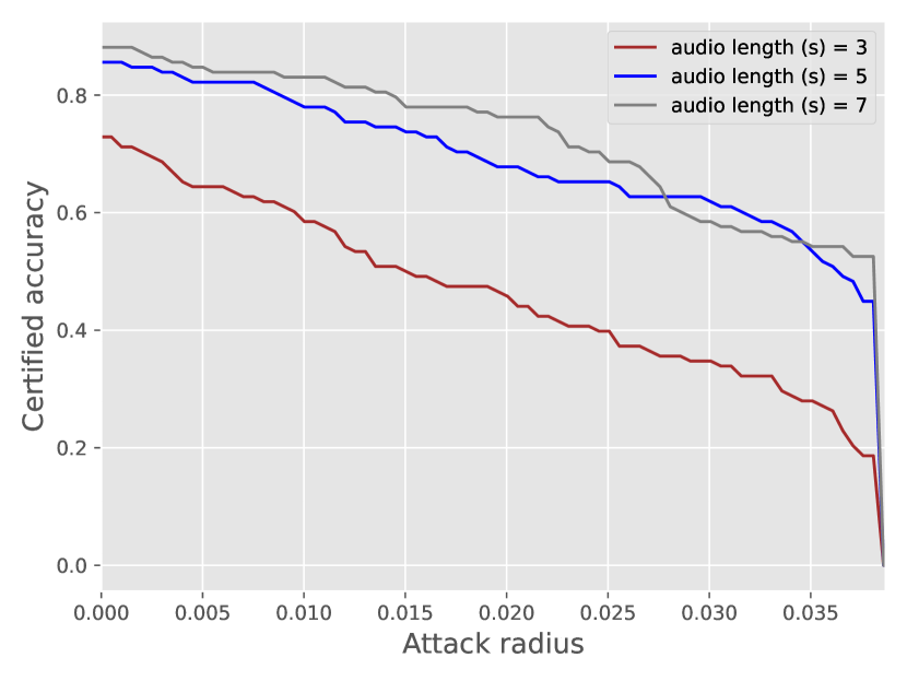
(c) Dependency on the audio length $n$.

Figure 10: Pyannote model. Classification setting. Dependency of certified accuracy on $M$ and number of presented in enrollment set classes.

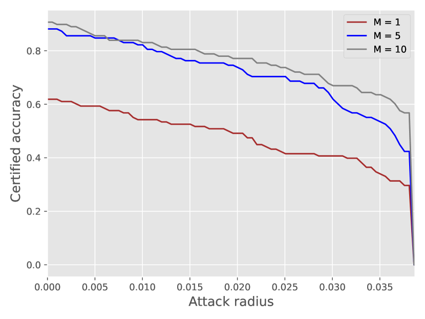
(a) Dependency on $M$

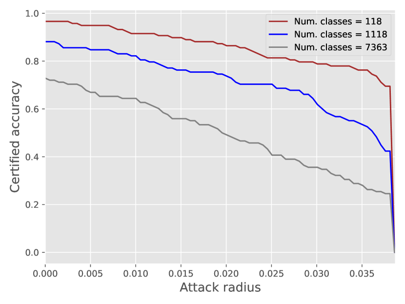
(b) Dependency on number of speakers.

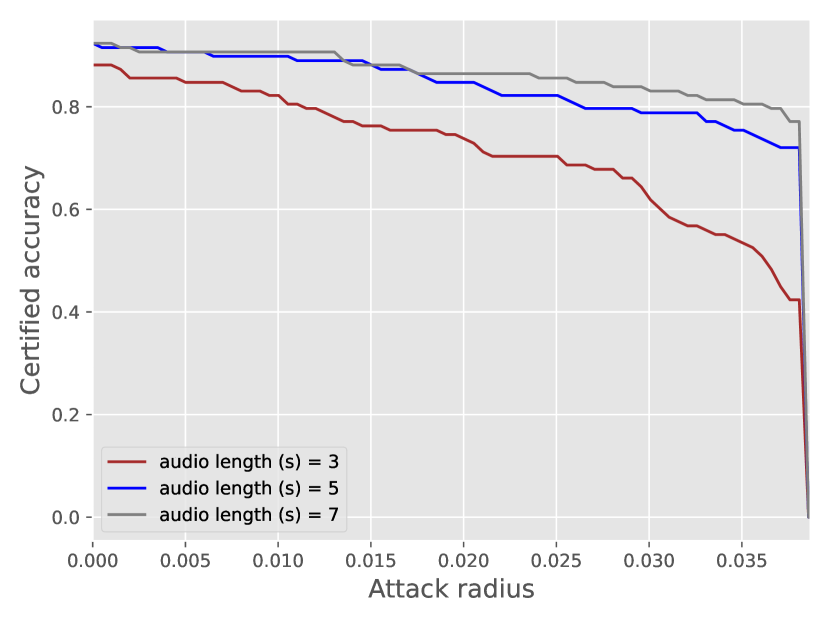
(c) Dependency on the audio length.

Figure 11: ECAPA-TDNN model. Classification setting. Dependency of certified accuracy on $M$ and number of presented in enrollment set classes.

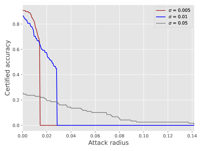
(a) Wespeaker

(b) CAM++

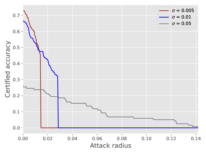
(c) ERes2Net

Figure 12: Classification setting. Dependency of certified accuracy on $\sigma$. Comparison of SE and our approaches for several models. $N_{\text{max}}=5000$.

References

- Andriushchenko and Flammarion [2020] M. Andriushchenko and N. Flammarion. Understanding and improving fast adversarial training. Advances in Neural Information Processing Systems, 33:16048–16059, 2020.
- Apostolidis and Papakostas [2021] K. D. Apostolidis and G. A. Papakostas. A survey on adversarial deep learning robustness in medical image analysis. Electronics, 10(17):2132, 2021.
- Athalye et al. [2018] A. Athalye, N. Carlini, and D. Wagner. Obfuscated gradients give a false sense of security: Circumventing defenses to adversarial examples. In International conference on machine learning, pages 274–283. PMLR, 2018.
- Bredin et al. [2020] H. Bredin, R. Yin, J. M. Coria, G. Gelly, P. Korshunov, M. Lavechin, D. Fustes, H. Titeux, W. Bouaziz, and M.-P. Gill. Pyannote. audio: neural building blocks for speaker diarization. In ICASSP 2020-2020 IEEE International Conference on Acoustics, Speech and Signal Processing (ICASSP), pages 7124–7128. IEEE, 2020.
- Chen et al. [2023] Y. Chen, S. Zheng, H. Wang, L. Cheng, Q. Chen, and J. Qi. An enhanced res2net with local and global feature fusion for speaker verification. arXiv preprint arXiv:2305.12838, 2023.
- Cheng et al. [2017] C.-H. Cheng, G. Nührenberg, and H. Ruess. Maximum resilience of artificial neural networks. In International Symposium on Automated Technology for Verification and Analysis, pages 251–268. Springer, 2017.
- Chung et al. [2018] J. S. Chung, A. Nagrani, and A. Zisserman. Voxceleb2: Deep speaker recognition. arXiv preprint arXiv:1806.05622, 2018.
- Clopper and Pearson [1934] C. J. Clopper and E. S. Pearson. The use of confidence or fiducial limits illustrated in the case of the binomial. Biometrika, 26(4):404–413, 1934.
- Cohen et al. [2019] J. Cohen, E. Rosenfeld, and Z. Kolter. Certified adversarial robustness via randomized smoothing. In International Conference on Machine Learning, pages 1310–1320. PMLR, 2019.
- Deng et al. [2023] J. Deng et al. V-Cloak: Intelligibility-, naturalness-& Timbre-PreservingReal-Time voice anonymization. In 32nd USENIX Security Symposium (USENIX Security 23), pages 5181–5198, 2023.
- Deng et al. [2020] Y. Deng, X. Zheng, T. Zhang, C. Chen, G. Lou, and M. Kim. An analysis of adversarial attacks and defenses on autonomous driving models. In 2020 IEEE international conference on pervasive computing and communications (PerCom), pages 1–10. IEEE, 2020.
- Desplanques et al. [2020] B. Desplanques, J. Thienpondt, and K. Demuynck. Ecapa-tdnn: Emphasized channel attention, propagation and aggregation in tdnn based speaker verification. arXiv preprint arXiv:2005.07143, 2020.
- Fan et al. [2023] M. Fan, C. Chen, C. Wang, W. Zhou, and J. Huang. On the robustness of split learning against adversarial attacks. arXiv preprint arXiv:2307.07916, 2023.
- Goodfellow et al. [2015] I. J. Goodfellow, J. Shlens, and C. Szegedy. Explaining and harnessing adversarial examples. In Y. Bengio and Y. LeCun, editors, ICLR, 2015.
- Gowal et al. [2019] S. Gowal, K. D. Dvijotham, R. Stanforth, R. Bunel, C. Qin, J. Uesato, R. Arandjelovic, T. Mann, and P. Kohli. Scalable verified training for provably robust image classification. In Proceedings of the IEEE/CVF International Conference on Computer Vision, pages 4842–4851, 2019.
- Hayes [2020] J. Hayes. Extensions and limitations of randomized smoothing for robustness guarantees. In Proceedings of the IEEE/CVF Conference on Computer Vision and Pattern Recognition Workshops, 2020.
- Hermans et al. [2017] A. Hermans, L. Beyer, and B. Leibe. In defense of the triplet loss for person re-identification. arXiv preprint arXiv:1703.07737, 2017.
- Hoeffding [1994] W. Hoeffding. Probability inequalities for sums of bounded random variables. In The collected works of Wassily Hoeffding, pages 409–426. Springer, 1994.
- Inkawhich et al. [2019] N. Inkawhich, W. Wen, H. H. Li, and Y. Chen. Feature space perturbations yield more transferable adversarial examples. In Proceedings of the IEEE/CVF Conference on Computer Vision and Pattern Recognition, pages 7066–7074, 2019.
- Kaziakhmedov et al. [2019] E. Kaziakhmedov, K. Kireev, G. Melnikov, M. Pautov, and A. Petiushko. Real-world attack on mtcnn face detection system. In 2019 International Multi-Conference on Engineering, Computer and Information Sciences (SIBIRCON), pages 0422–0427. IEEE, 2019.
- Komkov and Petiushko [2021] S. Komkov and A. Petiushko. Advhat: Real-world adversarial attack on arcface face id system. In 2020 25th International Conference on Pattern Recognition (ICPR), pages 819–826. IEEE, 2021.
- Li et al. [2023] L. Li, T. Xie, and B. Li. Sok: Certified robustness for deep neural networks. In 2023 IEEE symposium on security and privacy (SP), pages 1289–1310. IEEE, 2023.
- Li et al. [2021] L. Li et al. Tss: Transformation-specific smoothing for robustness certification. In Proceedings of the 2021 ACM SIGSAC Conference on Computer and Communications Security, pages 535–557, 2021.
- Li et al. [2020] Z. Li et al. Practical adversarial attacks against speaker recognition systems. In Proceedings of the 21st international workshop on mobile computing systems and applications, pages 9–14, 2020.
- Lyu et al. [2020] Z. Lyu, C.-Y. Ko, Z. Kong, N. Wong, D. Lin, and L. Daniel. Fastened crown: Tightened neural network robustness certificates. In Proceedings of the AAAI Conference on Artificial Intelligence, volume 34, pages 5037–5044, 2020.
- Meng et al. [2021] Q. Meng, S. Zhao, Z. Huang, and F. Zhou. Magface: A universal representation for face recognition and quality assessment. In Proceedings of the IEEE/CVF conference on computer vision and pattern recognition, pages 14225–14234, 2021.
- Muravev and Petiushko [2021] N. Muravev and A. Petiushko. Certified robustness via randomized smoothing over multiplicative parameters of input transformations. arXiv preprint arXiv:2106.14432, 2021.
- Nagrani et al. [2017] A. Nagrani, J. S. Chung, and A. Zisserman. Voxceleb: a large-scale speaker identification dataset. arXiv preprint arXiv:1706.08612, 2017.
- Olivier and Raj [2021] R. Olivier and B. Raj. Sequential randomized smoothing for adversarially robust speech recognition. In M.-F. Moens, X. Huang, L. Specia, and S. W.-t. Yih, editors, Proceedings of the 2021 Conference on Empirical Methods in Natural Language Processing, Nov. 2021.
- Pautov et al. [2022] M. Pautov, O. Kuznetsova, N. Tursynbek, A. Petiushko, and I. Oseledets. Smoothed embeddings for certified few-shot learning. Advances in Neural Information Processing Systems, 35:24367–24379, 2022.
- Pulina and Tacchella [2010] L. Pulina and A. Tacchella. An abstraction-refinement approach to verification of artificial neural networks. In International Conference on Computer Aided Verification, pages 243–257. Springer, 2010.
- Qin et al. [2023] Z. Qin, W. Zhao, X. Yu, and X. Sun. Openvoice: Versatile instant voice cloning. arXiv preprint arXiv:2312.01479, 2023.
- Ravanelli et al. [2021] M. Ravanelli, T. Parcollet, P. Plantinga, A. Rouhe, S. Cornell, L. Lugosch, C. Subakan, N. Dawalatabad, A. Heba, J. Zhong, et al. Speechbrain: A general-purpose speech toolkit. arXiv preprint arXiv:2106.04624, 2021.
- Salman et al. [2019] H. Salman, J. Li, I. Razenshteyn, P. Zhang, H. Zhang, S. Bubeck, and G. Yang. Provably robust deep learning via adversarially trained smoothed classifiers. Advances in Neural Information Processing Systems, 32, 2019.
- Singla and Feizi [2020] S. Singla and S. Feizi. Second-order provable defenses against adversarial attacks. In International conference on machine learning, pages 8981–8991. PMLR, 2020.
- Snyder et al. [2018] D. Snyder, D. Garcia-Romero, G. Sell, D. Povey, and S. Khudanpur. X-vectors: Robust dnn embeddings for speaker recognition. In 2018 IEEE international conference on acoustics, speech and signal processing (ICASSP), pages 5329–5333. IEEE, 2018.
- Szegedy et al. [2013] C. Szegedy, W. Zaremba, I. Sutskever, J. Bruna, D. Erhan, I. Goodfellow, and R. Fergus. Intriguing properties of neural networks. arXiv preprint arXiv:1312.6199, 2013.
- Wan et al. [2018] L. Wan, Q. Wang, A. Papir, and I. L. Moreno. Generalized end-to-end loss for speaker verification. In 2018 IEEE International Conference on Acoustics, Speech and Signal Processing (ICASSP), pages 4879–4883. IEEE, 2018.
- Wang and Liu [2021] F. Wang and H. Liu. Understanding the behaviour of contrastive loss. In Proceedings of the IEEE/CVF conference on computer vision and pattern recognition, pages 2495–2504, 2021.
- Wang et al. [2023a] H. Wang, C. Liang, S. Wang, Z. Chen, B. Zhang, X. Xiang, Y. Deng, and Y. Qian. Wespeaker: A research and production oriented speaker embedding learning toolkit. In ICASSP 2023-2023 IEEE International Conference on Acoustics, Speech and Signal Processing (ICASSP), pages 1–5. IEEE, 2023a.
- Wang et al. [2023b] H. Wang, S. Zheng, Y. Chen, L. Cheng, and Q. Chen. Cam++: A fast and efficient network for speaker verification using context-aware masking. arXiv preprint arXiv:2303.00332, 2023b.
- Wang et al. [2023c] Y. Wang, T. Sun, S. Li, X. Yuan, W. Ni, E. Hossain, and H. V. Poor. Adversarial attacks and defenses in machine learning-empowered communication systems and networks: A contemporary survey. IEEE Communications Surveys & Tutorials, 2023c.
- Wu et al. [2021] H. Wu, X. Li, A. T. Liu, Z. Wu, H. Meng, and H.-Y. Lee. Improving the adversarial robustness for speaker verification by self-supervised learning. IEEE/ACM Transactions on Audio, Speech, and Language Processing, 30:202–217, 2021.
- Yamagishi et al. [2021] J. Yamagishi, X. Wang, M. Todisco, M. Sahidullah, J. Patino, A. Nautsch, X. Liu, K. A. Lee, T. Kinnunen, N. Evans, et al. Asvspoof 2021: accelerating progress in spoofed and deepfake speech detection. In ASVspoof 2021 Workshop-Automatic Speaker Verification and Spoofing Coutermeasures Challenge, 2021.
- Yang et al. [2020] G. Yang, T. Duan, J. E. Hu, H. Salman, I. Razenshteyn, and J. Li. Randomized smoothing of all shapes and sizes. In International Conference on Machine Learning, pages 10693–10705. PMLR, 2020.
- Yuan et al. [2021] Z. Yuan, J. Zhang, Y. Jia, C. Tan, T. Xue, and S. Shan. Meta gradient adversarial attack. In Proceedings of the IEEE/CVF International Conference on Computer Vision (ICCV), pages 7748–7757, 2021.
- Zhang et al. [2023] X. Zhang, X. Zhang, M. Sun, X. Zou, K. Chen, and N. Yu. Imperceptible black-box waveform-level adversarial attack towards automatic speaker recognition. Complex & Intelligent Systems, 9(1):65–79, 2023.