Multigrid method for nonlinear eigenvalue problems based on Newton iteration

Abstract

In this paper, a novel multigrid method based on Newton iteration is proposed to solve nonlinear eigenvalue problems. Instead of handling the eigenvalue $\lambda$ and eigenfunction $u$ separately, we treat the eigenpair $(\lambda,u)$ as one element in a product space $\mathbb{R}\times H_{0}^{1}(\Omega)$. Then in the presented multigrid method, only one discrete linear boundary value problem needs to be solved for each level of the multigrid sequence. Because we avoid solving large-scale nonlinear eigenvalue problems directly, the overall efficiency is significantly improved. The optimal error estimate and linear computational complexity can be derived simultaneously. In addition, we also provide an improved multigrid method coupled with a mixing scheme to further guarantee the convergence and stability of the iteration scheme. More importantly, we prove convergence for the residuals after each iteration step. For nonlinear eigenvalue problems, such theoretical analysis is missing from the existing literatures on the mixing iteration scheme.

1 Introduction

Solving large-scale nonlinear eigenvalue problems is a basic and challenging task in the field of scientific and engineering computing. Various practical problems reduce to solve nonlinear eigenvalue problems. For example, the Schrödinger-Newton equation which has been widely used to model the quantum state reduction harri , the Gross-Pitaevskii equation which describes Bose-Einstein condensates baowei , and the Kohn-Sham equation which is used to describe the electronic structure in quantum chemistry CancesChakirMaday ; Canceschakir . In this paper, we will study a class of nonlinear eigenvalue models with convex energy functional. It is quite difficult to solve such nonlinear eigenvalue problems whose computational work grows exponentially as the problem size increases. Additionally, there are far fewer available numerical methods for nonlinear eigenvalue problems than those for the boundary value problems.

In this study, we resort to the multigrid method to improve the solving efficiency for nonlinear eigenvalue problems. The multigrid method was first proposed by Fedorenko fedore in 1961. Later, Brandt brandt demonstrated the efficiency of the multigrid method, which was then a widely examined subject in the computational mathematics field. Subsequently, Hackbusch, Xu, and many others began to use the tool of functional analysis to analyze this algorithm Hackbusch_Book ; Xu ; Shaidurov , which made the multigrid method experience rapid development. As we know, the multigrid method is able to derive an approximate solution possessing the optimal error estimates with the linear computational complexity. For eigenvalue problems, the study on the multigrid method is relatively limited. Xu and Zhou XuZhou_2001 first designed a two-grid method for the linear eigenvalue problem. This algorithm requires solving a small-scale eigenvalue problem on a coarse mesh and a large-scale boundary value problem on a fine mesh. When the mesh sizes of the coarse mesh ($H$) and fine mesh ($h$) have an appropriate proportional relation ($H=\sqrt{h}$), the optimal estimate for the approximate solution can be derived. Later, Chen and Liu et al. chenliu extended the two-grid method to solve nonlinear eigenvalue problems using specially selected coarse and fine meshes. However, owing to the strict constrains on the ratio (i.e., $H=\sqrt{h}$), the two-grid method only performs on two mesh levels and cannot be used in the multigrid sequence.

To solve the nonlinear eigenvalue problems via the multigrid technique, the Newton iteration is adopted. In this paper, the eigenvalue $\lambda$ and eigenfunction $u$ are treated as one element in a product space $\mathbb{R}\times H_{0}^{1}(\Omega)$. Then, the nonlinear eigenvalue equation can be viewed as a special nonlinear equation defined in $\mathbb{R}\times H_{0}^{1}(\Omega)$. Next, based on the Newton iteration technique, we simply solve a linear boundary value problem in each layer of the multigrid sequence. Solving the large-scale nonlinear eigenvalue problem is avoided in our algorithm. Besides, the involved linearized boundary value problems can be solved quickly by many mature numerical algorithms, such as the classical multigrid method. Hence, the presented algorithm can significantly improve the solving efficiency for nonlinear eigenvalue problems. The well-posedness for these linearized boundary value problems and the convergence for our entire algorithm have been rigorously analyzed in this paper.

For the above-mentioned multigrid method, we find that the Newton iteration scheme may fail to converge for some complicated nonlinear eigenvalue models. In fact, this problem exists widely during the self-consistent field iteration for nonlinear eigenvalue problems. To derive a convergence result, the mixing scheme (or damping method) is introduced. The most widely used mixing scheme is Anderson acceleration, which is used to improve the convergence rate for fixed-point iterations. Anderson acceleration was first designed by D. G. Anderson in 1965 to solve the integral equation andersion . Subsequently, this technique was used to solve various models, such as, the self-consistent field iteration in electronic structure computations fang , flow problems vc1 ; vc2 , molecular interaction stasiak , etc. Anderson acceleration adopts the mixing scheme to make the fixed-point iterations converge for general equations. Despite its widespread applications, the first mathematical convergence result for linear and nonlinear problems did not appear until 2015 in Toth . For nonlinear eigenvalue problems, there is still no strictly theoretical analysis. In general, the mixing scheme is used in fixed-point iterations to accelerate the convergence rate. Thus, we use the mixing scheme in the Newton iteration scheme to design a more efficient multigrid method. By treating the nonlinear eigenvalue problem as a special nonlinear equation, we just solve a series of linearized boundary value problems derived from the Newton iteration scheme defined on a multigrid space sequence. Next, we mix the approximate solution in each iteration step to generate a more accurate approximation. More importantly, we can rigorously prove convergence for the residuals of the nonlinear eigenvalue problem after a one-time iteration step. This may provide some inspiration to prove the theoretical conclusions of the self-consistent field iteration for nonlinear eigenvalue problems.

The remainder of this paper is organized as follows. In Section 2, some preliminaries about the nonlinear eigenvalue problems and the corresponding finite element method are presented. In Section 3, we use the Newton iteration to solve the nonlinear eigenvalue problems and provide several useful error estimates. In Section 4, the multigrid method based on Newton iteration is introduced. In Section 5, we adopt the mixing scheme to provide an improved multigrid algorithm. Numerical experiments are presented in Section 6 to verify the theoretical results derived in this paper. Some concluding remarks are presented in the last section.

2 Preliminaries of nonlinear eigenvalue problems

In this section, we first introduce some standard notations for Sobolev space $W^{s,p}(\Omega)$ and the associated norm $\|\cdot\|_{s,p,\Omega}$ on a bounded domain $\Omega\in\mathbb{R}^{d}\ (d\geq 1)$. For $p=2$, we denote $\|\cdot\|_{s,\Omega}=\|\cdot\|_{s,2,\Omega}$, $H^{s}(\Omega)=W^{s,2}(\Omega)$ and $H_{0}^{1}(\Omega)=\{v\in H^{1}(\Omega):v|_{\partial\Omega}=0\}$. Hereafter, we use $\lesssim$, $\gtrsim$, $\approx$ to denote $\leq$, $\geq$, $=$ with a mesh-independent coefficient for simplicity.

In this paper, we focus on the nonlinear eigenvalue problems arising from the following variational problem:

$$I=\inf\{E(v),v\in H_{0}^{1}(\Omega),\int_{\Omega}v^{2}d\Omega=1\},$$ (1)

where the energy functional $E$ is defined by

$$E(v)=\dfrac{1}{2}a(v,v)+\dfrac{1}{2}\int_{\Omega}F(v^{2})d\Omega,$$

with

$$a(u,v)=\int_{\Omega}(\mathcal{A}\nabla u\cdot\nabla v+Vuv)d\Omega.$$

To simplify the notation, let us define $f(t)=F^{\prime}(t)$. Then, for all $v\in H_{0}^{1}(\Omega)$, $E^{\prime}(v)=A_{v}v$ holds with

$$A_{v}=-{\rm div}(\mathcal{A}\nabla\cdot)+V+f(v^{2}).$$ (2)

Next, applying the Lagrange multiplier method to (1) yields the following nonlinear eigenvalue problem:

$$\left\{\begin{array}[]{rcl}A_{u}u&=&\lambda u,\ \ \text{ in }\Omega,\\ u&=&0,\ \ \ \ \text{ on }\partial\Omega,\\ \int_{\Omega}u^{2}d\Omega&=&1,\end{array}\right.$$ (3)

where $\lambda$ comes from the Lagrange multiplier of the constraint $\|u\|_{0}^{2}=1$.

For future theoretical analysis, we assume that the following conditions hold true (see CancesChakirMaday ; ChenZhou ):

• $\mathcal{A}$ is a symmetric positive-definite matrix;

• $V\in L^{p}(\Omega)$ for some $p>\max(1,d/2)$;

• $F\in C^{1}([0,\infty),\mathbb{R})\cap C^{2}((0,\infty),\mathbb{R})$ and $F^{\prime\prime}>0$ on $(0,\infty)$;

• $\exists\ 0\leq m<2\ \text{and}\ C\in\mathbb{R}_{+},\ \text{s.t.}\ \forall t\geq 0,\ |F^{\prime}(t)|\leq C(1+t^{m})$;

• $F^{\prime\prime}(t)t$ is locally bounded in $[0,\infty)$;

• $\exists\ 1<r\leq 2$ and $0\leq s\leq 5-r$ such that $\forall a>0,\exists\ C\in\mathbb{R}_{+},\ \text{s.t.}\ \forall\ 0<t_{1}\leq a,\ \forall\ t_{2}\in\mathbb{R},$

  $$|f(t_{2}^{2})t_{2}-f(t_{1}^{2})t_{1}-2f^{\prime}(t_{1}^{2})t_{1}^{2}(t_{2}-t_{1})|\leq C(1+|t_{2}|^{s})|t_{2}-t_{1}|^{r};$$

• $\exists\ 0\leq q<1\ \text{and}\ C\in\mathbb{R}_{+},\ \text{s.t.}\ \forall t\geq 0,\ |f^{\prime}(t)|+|f^{\prime\prime}(t)t|\leq C(1+t^{q})$.

In the remainder of this section, we present two lemmas for the nonlinear eigenvalue problem (3), and the detailed proof can be found in CancesChakirMaday .

Lemma 1

There exist $M\in\mathbb{R}_{+}$ and $\beta>0$ such that for all $v\in H_{0}^{1}(\Omega)$, there holds

$$0\leq((A_{u}-\lambda)v,v)\leq M\|v\|_{1}^{2},$$ (4)

and

$$\beta\|v\|_{1}^{2}\leq((E^{\prime\prime}(u)-\lambda)v,v)\leq M\|v\|_{1}^{2},$$ (5)

where $E^{\prime\prime}(u)$ has the following form

$$(E^{\prime\prime}(u)w,v)=(A_{u}w,v)+2(f^{\prime}(u^{2})u^{2}w,v).$$ (6)

Now, we introduce the finite element method for the nonlinear eigenvalue problem (3). To use the finite element method, we define the variational form for (3) as follows: Find $(\lambda,u)\in\mathbb{R}\times H_{0}^{1}(\Omega)$ such that $\|u\|_{0}=1$ and

$$(\mathcal{A}\nabla u,\nabla v)+(Vu+f(u^{2})u,v)=\lambda(u,v),\quad\forall v\in H_{0}^{1}(\Omega).$$ (7)

Next, we define the finite element space $V_{h}$ on a triangulation $\mathcal{T}_{h}$. The finite element space $V_{h}$ is composed of piecewise polynomials such that $V_{h}\subset H_{0}^{1}(\Omega)$ and

$$\lim_{h\rightarrow 0}\inf_{v_{h}\in V_{h}}\|w-v_{h}\|_{1}=0,\ \ \ \forall w\in H_{0}^{1}(\Omega).$$ (8)

Based on the finite element space $V_{h}$, we can derive the finite element solution for (7) by solving the discrete nonlinear eigenvalue problem as follows: Find $(\lambda_{h},u_{h})\in\mathbb{R}\times V_{h}$ such that $\|u_{h}\|_{0}=1$ and

$$(\mathcal{A}\nabla u_{h},\nabla v_{h})+(Vu_{h}+f(u_{h}^{2})u_{h},v_{h})=\lambda_{h}(u_{h},v_{h}),\quad\forall v_{h}\in V_{h}.$$ (9)

The standard error estimates for the finite element approximate eigenpair $(\lambda_{h},u_{h})$ are described in the following lemma.

Lemma 2

There exists $h_{0}>0$, such that for all $0<h<h_{0}$, the following error estimates hold true

$$\|u-u_{h}\|_{1}\lesssim\delta_{h}(u),$$ (10)

and

$$|\lambda-\lambda_{h}|\lesssim\|u-u_{h}\|_{1}^{2}+\|u-u_{h}\|_{L^{6/(5-2m)}},$$ (11)

where

$$\delta_{h}(u):=\inf_{v_{h}\in V_{h}}\|u-v_{h}\|_{1}.$$ (12)

3 Newton iteration for nonlinear eigenvalue problems

To introduce Newton iteration for nonlinear eigenvalue problem (7), we first give some symbols to simplify the description. Let us define

$$\langle\mathcal{F}(\lambda,u),v\rangle=(\mathcal{A}\nabla u,\nabla v)+(Vu+f(u^{2})u-\lambda u,v),\quad\forall v\in H_{0}^{1}(\Omega).$$ (13)

The Fréchet derivation of $\mathcal{F}$ with respect to $u$ at $(\lambda,u)$ is denoted by

$$\langle\mathcal{F}^{\prime}_{u}(\lambda,u)w,v\rangle = (\mathcal{A}\nabla w,\nabla v)+((V+f(u^{2})-\lambda)w,v)+2(f^{\prime}(u^{2})u^{2}w,v)$$ (14)

$$= (E^{\prime\prime}(u)w,v)-\lambda(w,v).$$

Next, we denote the product space $\mathbb{R}\times H_{0}^{1}(\Omega)$ by $X$. Let us define the norms in $X$ as

$$\|(\lambda,u)\|_{X}=|\lambda|+\|u\|_{1}\quad\text{and}\quad\|(\lambda,u)\|_{0}=|\lambda|+\|u\|_{0},\quad\forall(\lambda,u)\in X.$$ (15)

Let us define

$$\langle\mathcal{G}(\lambda,u),(\mu,v)\rangle=\langle\mathcal{F}(\lambda,u),v\rangle+\frac{1}{2}\mu(1-\int_{\Omega}u^{2}d\Omega),\quad\forall(\mu,v)\in X.$$ (16)

Obviously, the nonlinear eigenvalue problem (7) is equivalent to the following nonlinear equation defined in the product space $X$: Find $(\lambda,u)\in X$ such that

$$\langle\mathcal{G}(\lambda,u),(\mu,v)\rangle=0,\quad\forall(\mu,v)\in X.$$ (17)

Similarly, to solve (17) using the finite element method, we also introduce a finite dimensional space $X_{h}:=\mathbb{R}\times V_{h}$ as the approximation for $X$. Then based on $X_{h}$, the finite element equation (9) is equivalent to the following nonlinear equation defined in the tensor product space $X_{h}$: Find $(\lambda_{h},u_{h})\in X_{h}$ such that

$$\langle\mathcal{G}(\lambda_{h},u_{h}),(\mu,v_{h})\rangle=0,\quad\forall(\mu,v_{h})\in X_{h}.$$ (18)

The Fréchet derivation of $\mathcal{G}$ at $(\lambda,u)$ is denoted by:

$$\langle\mathcal{G}^{\prime}(\lambda,u)(\gamma,w),(\mu,v)\rangle=\langle\mathcal{F}_{u}^{\prime}(\lambda,u)w,v\rangle-\gamma(u,v)-\mu(u,w),\quad\forall(\mu,v)\in X.$$ (19)

Next, we begin to introduce the Newton iteration for (18). Given an initial value $(\lambda^{(0)},u^{(0)})\in X_{h}$, the one step of the Newton iteration is defined as follows, which will generate a more accurate approximate solution: Find $(\lambda^{(1)},u^{(1)})\in X_{h}$ such that

$$\big{\langle}\mathcal{G}^{\prime}(\lambda^{(0)},u^{(0)})(\lambda^{(1)}-\lambda^{(0)},u^{(1)}-u^{(0)}),(\mu,v_{h})\big{\rangle}=-\big{\langle}\mathcal{G}(\lambda^{(0)},u^{(0)}),(\mu,v_{h})\big{\rangle},\forall(\mu,v_{h})\in X_{h}.$$ (20)

Based on the definitions (16) and (19), the linearized boundary value problem (20) can be rewritten as follows: Find $(\lambda^{(1)},u^{(1)})\in\mathbb{R}\times V_{h}$ such that for any $(\mu,v_{h})\in\mathbb{R}\times V_{h}$, there holds

$$\left\{\begin{array}[]{lll}a(\lambda^{(0)},u^{(0)};u^{(1)},v_{h})+b(u^{(0)};v_{h},\lambda^{(1)})&=&\langle\mathcal{F}^{\prime}_{u}(\lambda^{(0)},u^{(0)})u^{(0)},v_{h}\rangle\\ &&-\langle\mathcal{F}(\lambda^{(0)},u^{(0)}),v_{h}\rangle-\lambda^{(0)}(u^{(0)},v_{h}),\\ b(u^{(0)};u^{(1)},\mu)&=&-\mu/2-\mu(u^{(0)},u^{(0)})/2,\end{array}\right.$$ (24)

where

$$a(\lambda^{(0)},u^{(0)};u^{(1)},v_{h})=\langle\mathcal{F}^{\prime}_{u}(\lambda^{(0)},u^{(0)})u^{(1)},v_{h}\rangle,\ \ \ \ b(u^{(0)};u^{(1)},\mu)=-\mu(u^{(0)},u^{(1)}).$$

To guarantee the well-posedness of (20) and (24), an isomorphism property is proved in Theorem 3.1:

Theorem 3.1

Let $(\lambda,u)$ be the exact solution of (17). When the mesh size $h$ is sufficiently small, we can derive the following isomorphism properties for the operator $\mathcal{G}^{\prime}$:

$$\mathop{\sup}\limits_{(\mu,v)\in X}\dfrac{\langle\mathcal{G}^{\prime}(\lambda,u)(\gamma,w),(\mu,v)\rangle}{\|(\mu,v)\|_{X}} \gtrsim \|(\gamma,w)\|_{X},\quad\forall(\gamma,w)\in X,$$ (25)

and

$$\mathop{\sup}\limits_{(\mu,v)\in X_{h}}\dfrac{\langle\mathcal{G}^{\prime}(\lambda,u)(\gamma,w),(\mu,v)\rangle}{\|(\mu,v)\|_{X}} \gtrsim \|(\gamma,w)\|_{X},\quad\forall(\gamma,w)\in X_{h}.$$ (26)

For any $(\widehat{\lambda},\widehat{u})\in X$ such that $\|(\widehat{\lambda}-\lambda,\widehat{u}-u)\|_{X}$ is sufficiently small, we can also derive

$$\mathop{\sup}\limits_{(\mu,v)\in X_{h}}\dfrac{\langle\mathcal{G}^{\prime}(\widehat{\lambda},\widehat{u})(\gamma,w),(\mu,v)\rangle}{\|(\mu,v)\|_{X}} \gtrsim \|(\gamma,w)\|_{X},\quad\forall(\gamma,w)\in X_{h}.$$ (27)

Proof

Firstly, proving (25) is equivalent to prove that for any $(\tau,f)\in\mathbb{R}\times H^{-1}(\Omega)$, the following equation is uniquely solvable: Find $(\gamma,w)\in\mathbb{R}\times H_{0}^{1}(\Omega)$ such that

$$\left\{\begin{array}[]{ll}a(\lambda,u;w,v)+b(u;v,\gamma)=(f,v),&\forall v\in H_{0}^{1}(\Omega),\\ b(u;w,\mu)=\mu\tau,&\forall\mu\in\mathbb{R}.\end{array}\right.$$ (30)

According to the Brezzi theory Fortin , we just need to prove the following two conclusions:
(1) The following equation

$$a(\lambda,u;w,v)=(f,v),\quad\forall v\in V_{0},$$ (31)

is uniquely solvable in $V_{0}:=\{v\in H_{0}^{1}(\Omega):b(u;v,\mu)=0,\ \forall\mu\in\mathbb{R}\}$.
(2) The following inf-sup condition holds true

$$\inf_{\mu\in\mathbb{R}}\sup_{v\in H_{0}^{1}(\Omega)}\dfrac{b(u;v,\mu)}{\|v\|_{1}|\mu|}\geq k_{b},$$ (32)

for some constant $k_{b}>0$.

Firstly, from (5), we can easily find that (31) is uniquely solvable. Next, since $\|u\|_{0}=1$, taking $v=-\mu u$ leads to

$$\inf_{\mu\in\mathbb{R}}\sup_{v\in H_{0}^{1}(\Omega)}\dfrac{b(u;v,\mu)}{\|v\|_{1}|\mu|}=\frac{1}{\|u\|_{1}}=:k_{b}.$$

Then we derive the inf-sup condition (32). Thus, we can derive the well-posedness of (30) based on Brezzi theory, which further yields (25).

Next, we begin to prove the second formula (26). Based on (5), let us define the projection $P_{h}:H_{0}^{1}(\Omega)\rightarrow V_{h}$ by

$$a(\lambda,u;w,v-P_{h}v)=0,\quad\forall w\in V_{h},\ \forall v\in H_{0}^{1}(\Omega).$$ (33)

Using (5) and (33), we can derive

$$\|P_{h}v\|_{1}\lesssim\|v\|_{1},\quad\forall v\in H_{0}^{1}(\Omega),$$ (34)

and

$$\|v-P_{h}v\|_{0}\lesssim h\|v-P_{h}v\|_{1}\lesssim h\|v\|_{1},\quad\forall v\in H_{0}^{1}(\Omega).$$ (35)

Combining (25), (33), (34) and (35) leads to

$$\|(\gamma,w)\|_{X} \lesssim \mathop{\sup}\limits_{(\mu,v)\in X}\dfrac{\langle\mathcal{G}^{\prime}(\lambda,u)(\gamma,w),(\mu,v)\rangle}{\|(\mu,v)\|_{X}}$$ (36)

$$= \mathop{\sup}\limits_{(\mu,v)\in X}\dfrac{\langle\mathcal{G}^{\prime}(\lambda,u)(\gamma,w),(0,v-P_{h}v)\rangle+\langle\mathcal{G}^{\prime}(\lambda,u)(\gamma,w),(\mu,P_{h}v)\rangle}{\|(\mu,v)\|_{X}}$$

$$= \mathop{\sup}\limits_{(\mu,v)\in X}\dfrac{a(\lambda,u;w,v-P_{h}v)-\gamma(u,v-P_{h}v)+\langle\mathcal{G}^{\prime}(\lambda,u)(\gamma,w),(\mu,P_{h}v)\rangle}{\|(\mu,v)\|_{X}}$$

$$= \mathop{\sup}\limits_{(\mu,v)\in X}\dfrac{-\gamma(u,v-P_{h}v)+\langle\mathcal{G}^{\prime}(\lambda,u)(\gamma,w),(\mu,P_{h}v)\rangle}{\|(\mu,v)\|_{X}}$$

$$\lesssim \mathop{\sup}\limits_{(\mu,v)\in X}\dfrac{\gamma\|u\|_{0}\|v-P_{h}v\|_{0}+\langle\mathcal{G}^{\prime}(\lambda,u)(\gamma,w),(\mu,P_{h}v)\rangle}{\|(\mu,v)\|_{X}}$$

$$\lesssim \mathop{\sup}\limits_{(\mu,v)\in X}\dfrac{\gamma h\|v\|_{1}+\langle\mathcal{G}^{\prime}(\lambda,u)(\gamma,w),(\mu,P_{h}v)\rangle}{\|(\mu,v)\|_{X}}$$

$$\lesssim h\|(\gamma,w)\|_{X}+\mathop{\sup}\limits_{(\mu,v)\in X}\dfrac{\langle\mathcal{G}^{\prime}(\lambda,u)(\gamma,w),(\mu,P_{h}v)\rangle}{\|(\mu,v)\|_{X}}.$$

Thus, when the mesh size $h$ is small enough, we can obtain

$$\|(\gamma,w)\|_{X} \lesssim \mathop{\sup}\limits_{(\mu,v)\in X}\dfrac{\langle\mathcal{G}^{\prime}(\lambda,u)(\gamma,w),(\mu,P_{h}v)\rangle}{\|(\mu,v)\|_{X}}$$ (37)

$$\lesssim \mathop{\sup}\limits_{(\mu,v)\in X}\dfrac{\langle\mathcal{G}^{\prime}(\lambda,u)(\gamma,w),(\mu,P_{h}v)\rangle}{\|(\mu,P_{h}v)\|_{X}}$$

$$\lesssim \mathop{\sup}\limits_{(\mu,v)\in X_{h}}\dfrac{\langle\mathcal{G}^{\prime}(\lambda,u)(\gamma,w),(\mu,v)\rangle}{\|(\mu,v)\|_{X}},$$

which is just the second formula (26).

For the last formula (27), we first prove a Lipschitz continuity for $\mathcal{G}^{\prime}$ based on the assumptions presented in Section 2, Hölder inequality and the imbedding theorem (see Adams ):

$$\langle\mathcal{G}^{\prime}(\lambda,u)(\gamma,w),(\mu,v)\rangle-\langle\mathcal{G}^{\prime}(\widehat{\lambda},\widehat{u})(\gamma,w),(\mu,v)\rangle$$

$$= \big{(}(f(u^{2})-f(\widehat{u}^{2}))w,v\big{)}+((\widehat{\lambda}-\lambda)w,v)$$

$$+2\big{(}(f^{\prime}(u^{2})u^{2}-f^{\prime}(\widehat{u}^{2})\widehat{u}^{2})w,v\big{)}-\gamma(\widehat{u}-u,v)-\mu(\widehat{u}-u,w)$$

$$= 2\big{(}f^{\prime}(\xi^{2})\xi(u-\widehat{u})w,v\big{)}+((\widehat{\lambda}-\lambda)w,v)$$

$$+4\big{(}(f^{\prime\prime}(\xi^{2})\xi^{3}+f^{\prime}(\xi^{2})\xi)(u-\widehat{u})w,v\big{)}-\gamma(\widehat{u}-u,v)-\mu(\widehat{u}-u,w)$$

$$\lesssim \big{(}(1+\xi^{2q})\xi(u-\widehat{u})w,v\big{)}+((\widehat{\lambda}-\lambda)w,v)$$

$$+\big{(}(1+\xi^{2q})\xi(u-\widehat{u})w,v\big{)}-\gamma(\widehat{u}-u,v)-\mu(\widehat{u}-u,w)$$

$$\lesssim \|\xi\|_{0,4}\|u-\widehat{u}\|_{0,4}\|w\|_{0,4}\|v\|_{0,4}+\|\xi^{2q}\|_{0,3/q}\|\xi\|_{0,6}\|u-\widehat{u}\|_{0,6}\|w\|_{0,6}\|v\|_{0,6/(3-2q)}$$

$$+|\widehat{\lambda}-\lambda|\|w\|_{0}\|v\|_{0}+|\gamma|\|\widehat{u}-u\|_{0}\|v\|_{0}+|\mu|\|\widehat{u}-u\|_{0}\|w\|_{0}$$

$$\lesssim \|\xi\|_{1}\|u-\widehat{u}\|_{1}\|w\|_{1}\|v\|_{1}+\|\xi\|_{1}^{2q}\|\xi\|_{1}\|u-\widehat{u}\|_{1}\|w\|_{1}\|v\|_{1}$$

$$+|\widehat{\lambda}-\lambda|\|w\|_{0}\|v\|_{0}+|\gamma|\|\widehat{u}-u\|_{0}\|v\|_{0}+|\mu|\|\widehat{u}-u\|_{0}\|w\|_{0},$$

where $\xi=\tau u+(1-\tau)\widehat{u}$ with $\tau\in(0,1)$.

Thus, we can derive

$$\langle\mathcal{G}^{\prime}(\lambda,u)(\gamma,w),(\mu,v)\rangle-\langle\mathcal{G}^{\prime}(\widehat{\lambda},\widehat{u})(\gamma,w),(\mu,v)\rangle$$ (38)

$$\lesssim \|(\lambda-\widehat{\lambda},u-\widehat{u})\|_{X}\|(\gamma,w)\|_{X}\|(\mu,v)\|_{X}.$$

Let $\varepsilon$ be a sufficiently small constant and $\|(\lambda-\widehat{\lambda},u-\widehat{u})\|_{X}\leq\varepsilon$. Based on (26) and (38), for any $(\gamma,w)\in X_{h}$, we have

$$\|(\gamma,w)\|_{X} \lesssim \mathop{\sup}\limits_{(\mu,v)\in X_{h}}\dfrac{\varepsilon\|(\gamma,w)\|_{X}\|(\mu,v)\|_{X}+\langle\mathcal{G}^{\prime}(\widehat{\lambda},\widehat{u})(\gamma,w),(\mu,v)\rangle}{\|(\mu,v)\|_{X}}$$

$$\lesssim \varepsilon\|(\gamma,w)\|_{X}+\mathop{\sup}\limits_{(\mu,v)\in X_{h}}\dfrac{\langle\mathcal{G}^{\prime}(\widehat{\lambda},\widehat{u})(\gamma,w),(\mu,v)\rangle}{\|(\mu,v)\|_{X}}.$$

Then $(\ref{coercive of g3})$ can be derived using the same way as the proof process in (37). This completes the proof.

Next, in Theorem 3.2, we provide the estimate for the residual of the Newton iteration scheme (20).

Theorem 3.2

For any $(\lambda^{(0)},u^{(0)})\in X,(\lambda^{(1)},u^{(1)})\in X$, we can derive the following expansion

$$\langle\mathcal{G}(\lambda^{(1)},u^{(1)}),(\sigma,\eta)\rangle = \langle\mathcal{G}(\lambda^{(0)},u^{(0)}),(\sigma,\eta)\rangle+\langle\mathcal{G}^{\prime}(\lambda^{(0)},u^{(0)})(\lambda^{(1)}-\lambda^{(0)},u^{(1)}-u^{(0)}),(\sigma,\eta)\rangle$$ (39)

$$+~{}R\big{(}(\lambda^{(0)},u^{(0)}),(\lambda^{(1)},u^{(1)}),(\sigma,\eta)\big{)},\quad\quad\quad\quad\quad\quad\forall(\sigma,\eta)\in X,$$

where the residual $R\big{(}(\lambda^{(0)},u^{(0)}),(\lambda^{(1)},u^{(1)}),(\sigma,\eta)\big{)}$ satisfies the following estimate

$$\big{|}R\big{(}(\lambda^{(0)},u^{(0)}),(\lambda^{(1)},u^{(1)}),(\sigma,\eta)\big{)}\big{|}\lesssim\|(\lambda^{(0)}-\lambda^{(1)},u^{(0)}-u^{(1)})\|_{X}^{2}\|(\sigma,\eta)\|_{X}.$$

Proof

We prove this theorem through the Taylor expansion. Let us define

$$\eta(t)=\big{\langle}\mathcal{G}\big{(}(\lambda^{(0)},u^{(0)})+t\{(\lambda^{(1)},u^{(1)})-(\lambda^{(0)},u^{(0)})\}\big{)},(\sigma,\eta)\big{\rangle},\ \ \ t\in[0,1].$$ (40)

Obviously,

$$\eta(0)=\langle\mathcal{G}(\lambda^{(0)},u^{(0)}),(\sigma,\eta)\rangle\ \ \ \text{and}\ \ \ \eta(1)=\langle\mathcal{G}(\lambda^{(1)},u^{(1)}),(\sigma,\eta)\rangle.$$ (41)

The first order derivative and the second order derivative of $\eta(t)$ with respect to $t$ are listed as follows:

$$\eta^{\prime}(t) = \big{\langle}\mathcal{G}^{\prime}((\lambda^{(0)},u^{(0)})+t\{(\lambda^{(1)},u^{(1)})-(\lambda^{(0)},u^{(0)})\})((\lambda^{(1)},u^{(1)})-(\lambda^{(0)},u^{(0)})),(\sigma,\eta)\big{\rangle}$$ (42)

$$= \big{\langle}\mathcal{F}_{u}^{\prime}\big{(}(\lambda^{(0)},u^{(0)})+t\{(\lambda^{(1)},u^{(1)})-(\lambda^{(0)},u^{(0)})\}\big{)}(u^{(1)}-u^{(0)}),\eta\big{\rangle}$$

$$-(\lambda^{(1)}-\lambda^{(0)})(u^{(0)}+t(u^{(1)}-u^{(0)}),\eta)-\sigma(u^{(0)}+t(u^{(1)}-u^{(0)}),u^{(1)}-u^{(0)})$$

$$= (\mathcal{A}\nabla(u^{(1)}-u^{(0)}),\nabla\eta)+\big{(}(u^{(0)}+f((u^{(0)}+t(u^{(1)}-u^{(0)}))^{2}))(u^{(1)}-u^{(0)}),\eta\big{)}$$

$$-\big{(}(\lambda^{(0)}+t(\lambda^{(1)}-\lambda^{(0)}))(u^{(1)}-u^{(0)}),\eta\big{)}$$

$$+2\big{(}f^{\prime}((u^{(0)}+t(u^{(1)}-u^{(0)}))^{2})(u^{(0)}+t(u^{(1)}-u^{(0)}))^{2}(u^{(1)}-u^{(0)}),\eta\big{)}$$

$$-(\lambda^{(1)}-\lambda^{(0)})(u^{(0)}+t(u^{(1)}-u^{(0)}),\eta)-\sigma(u^{(0)}+t(u^{(1)}-u^{(0)}),u^{(1)}-u^{(0)}),$$

and

$$\eta^{\prime\prime}(t) = -2(\lambda^{(1)}-\lambda^{(0)})(u^{(1)}-u^{(0)},\eta)-\sigma(u^{(1)}-u^{(0)},u^{(1)}-u^{(0)})$$ (43)

$$+6\big{(}f^{\prime}\big{(}(u^{(0)}+t(u^{(1)}-u^{(0)}))^{2}\big{)}\big{(}u^{(0)}+t(u^{(1)}-u^{(0)})\big{)}(u^{(1)}-u^{(0)})^{2},\eta\big{)}$$

$$+4\big{\langle}f^{\prime\prime}\big{(}(u^{(0)}+t(u^{(1)}-u^{(0)}))^{2}\big{)}\big{(}u^{(0)}+t(u^{(1)}-u^{(0)})\big{)}^{3}(u^{(1)}-u^{(0)})^{2},\eta\big{\rangle}.$$

For the nonlinear terms involved in (43), we have the following estimates

$$\big{|}\big{(}f^{\prime}\big{(}(u^{(0)}+t(u^{(1)}-u^{(0)}))^{2}\big{)}\big{(}u^{(0)}+t(u^{(1)}-u^{(0)})\big{)}(u^{(1)}-u^{(0)})^{2},\eta\big{)}\big{|}$$ (44)

$$\lesssim \big{|}\big{(}\big{(}1+(u^{(0)}+t(u^{(1)}-u^{(0)}))^{2q}\big{)}\big{(}u^{(0)}+t(u^{(1)}-u^{(0)})\big{)}(u^{(1)}-u^{(0)})^{2},\eta\big{)}\big{|}$$

$$\lesssim \big{|}\big{(}(u^{(0)}+t(u^{(1)}-u^{(0)}))(u^{(1)}-u^{(0)})^{2},\eta\big{)}$$

$$+\big{(}(u^{(0)}+t(u^{(1)}-u^{(0)}))^{2q}(u^{(0)}+t(u^{(1)}-u^{(0)}))(u^{(1)}-u^{(0)})^{2},\eta\big{)}\big{|}$$

$$\lesssim \|u^{(0)}+t(u^{(1)}-u^{(0)})\|_{0,4}\|u^{(1)}-u^{(0)}\|_{0,4}^{2}\|\eta\|_{0,4}$$

$$+\|(u^{(0)}+t(u^{(1)}-u^{(0)}))^{2q}\|_{0,3/q}\|u^{(0)}+t(u^{(1)}-u^{(0)})\|_{0,6}\|u^{(1)}-u^{(0)}\|_{0,6}^{2}\|\eta\|_{0,6/(3-2q)}$$

$$\lesssim \|u^{(0)}+t(u^{(1)}-u^{(0)})\|_{0,4}\|u^{(1)}-u^{(0)}\|_{0,4}^{2}\|\eta\|_{0,4}$$

$$+\|u^{(0)}+t(u^{(1)}-u^{(0)})\|_{0,6}^{2q}\|u^{(0)}+t(u^{(1)}-u^{(0)})\|_{0,6}\|u^{(1)}-u^{(0)}\|_{0,6}^{2}\|\eta\|_{0,6/(3-2q)}$$

$$\lesssim \|u^{(0)}+t(u^{(1)}-u^{(0)})\|_{1}\|u^{(1)}-u^{(0)}\|_{1}^{2}\|\eta\|_{1}$$

$$+\|u^{(0)}+t(u^{(1)}-u^{(0)})\|_{1}^{2q}\|u^{(0)}+t(u^{(1)}-u^{(0)})\|_{1}\|u^{(1)}-u^{(0)}\|_{1}^{2}\|\eta\|_{1}$$

$$\lesssim \|u^{(1)}-u^{(0)}\|_{1}^{2}\|\eta\|_{1},$$

and

$$\big{|}\big{\langle}f^{\prime\prime}\big{(}(u^{(0)}+t(u^{(1)}-u^{(0)}))^{2}\big{)}\big{(}u^{(0)}+t(u^{(1)}-u^{(0)})\big{)}^{3}(u^{(1)}-u^{(0)})^{2},\eta\big{\rangle}\big{|}$$ (45)

$$\lesssim \big{|}\big{(}(1+(u^{(0)}+t(u^{(1)}-u^{(0)}))^{2q}\big{)}\big{(}u^{(0)}+t(u^{(1)}-u^{(0)})\big{)}(u^{(1)}-u^{(0)})^{2},\eta)\big{|}$$

$$\lesssim \|u^{(1)}-u^{(0)}\|_{1}^{2}\|\eta\|_{1},$$

where the Hölder inequality and the imbedding theorem are used.

Based on (43), (44) and (45), we can derive

$$|\eta^{\prime\prime}(t)| \lesssim |\lambda^{(1)}-\lambda^{(0)}|\|u^{(1)}-u^{(0)}\|_{0}\|\eta\|_{0}+|\sigma|\|u^{(1)}-u^{(0)}\|_{0}^{2}+\|u^{(1)}-u^{(0)}\|_{1}^{2}\|\eta\|_{1}$$ (46)

$$\lesssim \|(\lambda^{(0)}-\lambda^{(1)},u^{(0)}-u^{(1)})\|_{X}^{2}\|(\sigma,\eta)\|_{X}.$$

Thus, using (46) and the following Taylor expansion:

$$\eta(1)=\eta(0)+\eta^{\prime}(0)+\int_{0}^{1}\eta^{\prime\prime}(t)(1-t)dt,$$

we can derive

$$\langle\mathcal{G}(\lambda^{(1)},u^{(1)}),(\sigma,\eta)\rangle = \langle\mathcal{G}(\lambda^{(0)},u^{(0)}),(\sigma,\eta)\rangle+\langle\mathcal{G}^{\prime}(\lambda^{(0)},u^{(0)})((\lambda^{(1)},u^{(1)})-(\lambda^{(0)},u^{(0)})),(\sigma,\eta)\rangle$$

$$+R((\lambda^{(0)},u^{(0)}),(\lambda^{(1)},u^{(1)}),(\sigma,\eta))$$

with the residual

$$|R((\lambda^{(0)},u^{(0)}),(\lambda^{(1)},u^{(1)}),(\sigma,\eta))|\lesssim\|(\lambda^{(0)}-\lambda^{(1)},u^{(0)}-u^{(1)})\|_{X}^{2}\|(\sigma,\eta)\|_{X}.$$

Then the proof is completed.

4 Multigrid method for nonlinear eigenvalue problems based on Newton iteration

In this section, a novel multigrid method is proposed for solving the nonlinear eigenvalue problems based on the Newton iteration. To design the multigrid method, let us construct a nested sequence of finite element spaces based on a nested multigrid sequence in the first step. The sequence of meshes is denoted by $\{\mathcal{T}_{h_{k}}\}_{k=1}^{n}$. For any two consecutive meshes $\mathcal{T}_{h_{k}}$ and $\mathcal{T}_{h_{k-1}}(k\geq 2)$, $\mathcal{T}_{h_{k}}$ is produced through a one-time uniform refinement form $\mathcal{T}_{h_{k-1}}$. The corresponding mesh sizes satisfy the following conditions:

$$h_{k}\approx\dfrac{1}{\beta}h_{k-1},\quad k=2,\cdots,n,$$ (47)

where the refinement index $\beta>1$. Meanwhile, the following approximate relationship holds true:

$$\delta_{h_{k}}(u)\approx\dfrac{1}{\beta}\delta_{h_{k-1}}(u),\quad k=2,\cdots,n.$$ (48)

Based on the multigrid sequence $\{\mathcal{T}_{h_{k}}\}_{k=1}^{n}$, we denote the corresponding sequence of finite element spaces by:

$$V_{h_{1}}\subset V_{h_{2}}\subset\cdots\subset V_{h_{n}}\subset H_{0}^{1}(\Omega),$$ (49)

and denote the sequence of tensor product finite element spaces by:

$$X_{h_{1}}\subset X_{h_{2}}\subset\cdots\subset X_{h_{n}}\subset X.$$ (50)

4.1 One step of the multigrid method

To describe the multigrid method more clearly, we first introduce how to perform one step of the Newton iteration.

For two consecutive finite element spaces $X_{h_{k}}$ and $X_{h_{k+1}}$, assume that we have obtained an approximate solution $(\lambda^{h_{k}},u^{h_{k}})\in X_{h_{k}}$, Algorithm 4.1 shows the procedure for obtaining a new approximate solution $(\lambda^{h_{k+1}},u^{h_{k+1}})\in X_{h_{k+1}}$.

Algorithm 4.1

One step of the multigrid method

1. Assume that we have obtained an approximate solution $(\lambda^{h_{k}},u^{h_{k}})\in X_{h_{k}}$.

2. Solve the linearized equation derived from Newton iteration in the finite element space $X_{h_{k+1}}$: Find $(\lambda^{h_{k+1}},u^{h_{k+1}})\in X_{h_{k+1}}$ such that for any $(\mu,v_{h_{k+1}})\in X_{h_{k+1}}$, there holds

   $$\langle\mathcal{G}^{\prime}(\lambda^{h_{k}},u^{h_{k}})(\lambda^{h_{k+1}},u^{h_{k+1}}),(\mu,v_{h_{k+1}})\rangle$$ (51)

   $$= -\langle\mathcal{G}(\lambda^{h_{k}},u^{h_{k}}),(\mu,v_{h_{k+1}})\rangle+\langle\mathcal{G}^{\prime}(\lambda^{h_{k}},u^{h_{k}})(\lambda^{h_{k}},u^{h_{k}}),(\mu,v_{h_{k+1}})\rangle.$$

   The equation (51) can be solved by the mixed finite element method in the following form: Find $(\lambda^{h_{k+1}},u^{h_{k+1}})\in\mathbb{R}\times V_{h_{k+1}}$ such that for any $(\mu,v_{h_{k+1}})\in\mathbb{R}\times V_{h_{k+1}}$, there holds

   $$\left\{\begin{array}[]{lll}a(\lambda^{h_{k}},u^{h_{k}};u^{h_{k+1}},v_{h_{k+1}})+b(u^{h_{k}};v_{h_{k+1}},\lambda^{h_{k+1}})&=&\langle\mathcal{F}_{u}^{\prime}(\lambda^{h_{k}},u^{h_{k}})u^{h_{k}},v_{h_{k+1}}\rangle\\ &&-\langle\mathcal{F}(\lambda^{h_{k}},u^{h_{k}}),v_{h_{k+1}}\rangle-\lambda^{h_{k}}(u^{h_{k}},v_{h_{k+1}}),\\ b(u^{h_{k}};u^{h_{k+1}},\mu)&=&-\mu/2-\mu(u^{h_{k}},u^{h_{k}})/2.\end{array}\right.$$

In order to simplify the notation, we use the following symbol to denote the above two solving steps:

$$(\lambda^{h_{k+1}},u^{h_{k+1}})=Newton_{-}Iteration(\lambda^{h_{k}},u^{h_{k}},X_{h_{k+1}}).$$

Next, we can prove that the new approximate solution $(\lambda^{h_{k+1}},u^{h_{k+1}})\in X_{h_{k+1}}$ derived by Algorithm 4.1 has a better accuracy than $(\lambda^{h_{k}},u^{h_{k}})\in X_{h_{k}}$. The detailed conclusion is presented in Theorem 4.1.

Theorem 4.1

After implementing Algorithm 4.1, the new approximate solution $(\lambda^{h_{k+1}},u^{h_{k+1}})$ has the following error estimate

$$\|(\lambda-\lambda^{h_{k+1}},u-u^{h_{k+1}})\|_{X}\lesssim\delta_{h_{k+1}}(u)+\|(\lambda-\lambda^{h_{k}},u-u^{h_{k}})\|_{X}^{2}.$$

Proof

We use $(\lambda_{h_{k+1}},u_{h_{k+1}})$ to denote the standard finite element solution of (9), that is $(\lambda_{h_{k+1}},u_{h_{k+1}})$ satisfies

$$(\mathcal{A}\nabla u_{h_{k+1}},\nabla v_{h_{k+1}})+(Vu_{h_{k+1}},v_{h_{k+1}})+(f(u_{h_{k+1}}^{2})u_{h_{k+1}},v_{h_{k+1}})$$

$$= \lambda_{h_{k+1}}(u_{h_{k+1}},v_{h_{k+1}}),\quad\forall v_{h_{k+1}}\in V_{h_{k+1}},$$

or equivalently

$$\langle\mathcal{G}(\lambda_{h_{k+1}},u_{h_{k+1}}),(\mu,v_{h_{k+1}})\rangle=0,\quad\forall(\mu,v_{h_{k+1}})\in X_{h_{k+1}}.$$ (53)

Combining (51) and (53) leads to

$$\big{\langle}\mathcal{G}^{\prime}(\lambda^{h_{k}},u^{h_{k}})(\lambda_{h_{k+1}}-\lambda^{h_{k+1}},u_{h_{k+1}}-u^{h_{k+1}}),(\mu,v_{h_{k+1}})\big{\rangle}$$ (54)

$$= \big{\langle}\mathcal{G}(\lambda^{h_{k}},u^{h_{k}}),(\mu,v_{h_{k+1}})\big{\rangle}+\big{\langle}\mathcal{G}^{\prime}(\lambda^{h_{k}},u^{h_{k}})(\lambda_{h_{k+1}}-\lambda^{h_{k}},u_{h_{k+1}}-u^{h_{k}}),(\mu,v_{h_{k+1}})\big{\rangle}$$

$$= -\big{\langle}\mathcal{G}(\lambda_{h_{k+1}},u_{h_{k+1}}),(\mu,v_{h_{k+1}})\big{\rangle}+\big{\langle}\mathcal{G}(\lambda^{h_{k}},u^{h_{k}}),(\mu,v_{h_{k+1}})\big{\rangle}$$

$$+\big{\langle}\mathcal{G}^{\prime}(\lambda^{h_{k}},u^{h_{k}})(\lambda_{h_{k+1}}-\lambda^{h_{k}},u_{h_{k+1}}-u^{h_{k}}),(\mu,v_{h_{k+1}})\big{\rangle}$$

$$= -R((\lambda^{h_{k}},u^{h_{k}}),(\lambda_{h_{k+1}},u_{h_{k+1}}),(\mu,v_{h_{k+1}})).$$

Combining (27), Theorem 3.2 and (54), we can derive

$$\|(\lambda_{h_{k+1}}-\lambda^{h_{k+1}},u_{h_{k+1}}-u^{h_{k+1}})\|_{X}\lesssim\|(\lambda_{h_{k+1}}-\lambda^{h_{k}},u_{h_{k+1}}-u^{h_{k}})\|_{X}^{2}.$$ (55)

Using the standard error estimates in Lemma 2 and (55), we can obtain

$$\|(\lambda-\lambda^{h_{k+1}},u-u^{h_{k+1}})\|_{X} \lesssim \|(\lambda-\lambda_{h_{k+1}},u-u_{h_{k+1}})\|_{X}+\|(\lambda_{h_{k+1}}-\lambda^{h_{k+1}},u_{h_{k+1}}-u^{h_{k+1}})\|_{X}$$

$$\lesssim \delta_{h_{k+1}}(u)+\|(\lambda-\lambda^{h_{k}},u-u^{h_{k}})\|_{X}^{2}.$$

Then we complete the proof.

4.2 Multigrid method based on Newton iteration

In this subsection, we introduce the multigrid method to solve the nonlinear eigenvalue problems. We use the following nested sequence of finite element spaces:

$$V_{h_{1}}\subset V_{h_{2}}\subset\cdots\subset V_{h_{n}}\subset H_{0}^{1}(\Omega),$$ (56)

and

$$X_{h_{1}}\subset X_{h_{2}}\subset\cdots\subset X_{h_{n}}\subset X.$$ (57)

The multigrid method is presented in Algorithm 4.2. The new algorithm requires solving the nonlinear eigenvalue problem directly in the initial space to obtain an initial value; then performing Algorithm 4.1 in the subsequent spaces. The approximate solution derived from the last space is used as the initial iterative value in the current space.

Algorithm 4.2

Multigrid method based on Newton iteration

1. Solve the following nonlinear eigenvalue problem directly in the initial space $V_{h_{1}}$: Find $(\lambda^{h_{1}},u^{h_{1}})\in\mathbb{R}\times V_{h_{1}}$ such that $\|u^{h_{1}}\|_{0}=1$ and

   $$(\mathcal{A}\nabla u^{h_{1}},\nabla v_{h_{1}})+(Vu^{h_{1}},v_{h_{1}})+(f((u^{h_{1}})^{2})u^{h_{1}},v_{h_{1}})=\lambda^{h_{1}}(u^{h_{1}},v_{h_{1}}),\quad\forall v_{h_{1}}\in V_{h_{1}}.$$

2. For $k=1,\cdots,n-1$, obtain a new approximate solution $(\lambda^{h_{k+1}},u^{h_{k+1}})\in X_{h_{k+1}}$ through

   $$(\lambda^{h_{k+1}},u^{h_{k+1}})=Newton_{-}Iteration(\lambda^{h_{k}},u^{h_{k}},X_{h_{k+1}}),$$

   End for.

3. Finally, we obtain the approximate solution $(\lambda^{h_{n}},u^{h_{n}})\in X_{h_{n}}$.

The error estimate for the final approximate solution $(\lambda^{h_{n}},u^{h_{n}})\in X_{h_{n}}$ derived by Algorithm 4.2 is presented in Theorem 4.2.

Theorem 4.2

After performing Algorithm 4.2, the final approximate solution $(\lambda^{h_{n}},u^{h_{n}})\in X_{h_{n}}$ satisfies the following error estimate

$$\|(\lambda-\lambda^{h_{n}},u-u^{h_{n}})\|_{X}\lesssim\delta_{h_{n}}(u).$$ (58)

Proof

We prove this theorem by the mathematical induction method. Since we solve the nonlinear eigenvalue problem directly in the initial space, using Lemma 2 leads to

$$\|(\lambda-{\lambda}^{h_{1}},u-{u}^{h_{1}})\|_{X}\lesssim\delta_{h_{1}}(u).$$

Assume that (58) holds true for $(\lambda^{h_{n-1}},{u}^{h_{n-1}})\in X_{h_{n-1}}$. According to Theorem 4.1, we can derive

$$\|(\lambda-{\lambda}^{h_{n}},u-{u}^{h_{n}})\|_{X}$$

$$\lesssim \delta_{h_{n}}(u)+\|(\lambda-\lambda^{h_{n-1}},u-u^{h_{n-1}})\|_{X}^{2}$$

$$\lesssim \delta_{h_{n}}(u)+\delta_{h_{n-1}}^{2}(u)$$

$$\lesssim \delta_{h_{n}}(u).$$

So (58) also holds true for $(\lambda^{h_{n}},{u}^{h_{n}})\in X_{h_{n}}$. Then the proof is completed.

4.3 Work estimate of Algorithm 4.2

In this subsection, we end Section 4 by estimating the computational work of Algorithm 4.2 briefly. Let us use $N_{k}$ to denote the dimensions of $V_{h_{k}}$. The dimensions of the sequence of finite element spaces satisfy

$$N_{k}\approx\beta^{d(k-n)}N_{n},\ \ \ k=1,2,\cdots,n.$$

Then the computational work of Algorithm 4.2 is presented in Theorem 4.3, which shows that Algorithm 4.2 has linear computational complexity.

Theorem 4.3

Assume that solving the nonlinear eigenvalue problem directly in the initial space $V_{h_{1}}$ needs work $\mathcal{O}(M_{h_{1}})$, and solving the linearized boundary value problem (51) in $V_{h_{k}}$ needs work $\mathcal{O}(N_{k})$ for $k=2,3,\cdots,n$. Then the total computational work of Algorithm 4.2 is $\mathcal{O}(N_{n}+M_{h_{1}})$. Furthermore, the linear computational complexity $\mathcal{O}(N_{n})$ can be derived provided $M_{h_{1}}\leq N_{n}$.

Proof

Let us use $W_{k}$ to denote the computational work of $V_{h_{k}}$. Then the computational work $W$ of Algorithm 4.2 can be estimated by:

$$W = \sum_{k=1}^{n}W_{k}=\mathcal{O}(M_{h_{1}}+\sum_{k=2}^{n}N_{k})$$

$$= \mathcal{O}(\sum_{k=2}^{n}\beta^{d(k-n)}N_{n}+M_{h_{1}})$$

$$= \mathcal{O}(N_{n}+M_{h_{1}}).$$

Then we get the desired conclusion $\mathcal{O}(N_{n}+M_{h_{1}})$, and when $M_{h_{1}}\leq N_{n}$, the total computational work changes to $\mathcal{O}(N_{n})$.

Remark 1

The linearized boundary value problem (51) can be solved efficiently by the multigrid method with linear computational complexity $\mathcal{O}(N_{k})$ (see e.g., Saddle-book ; Shaidurov ). Because the dimension of the initial space $V_{h_{1}}$ is small and independent of the final finite element space, it is easy to get $M_{h_{1}}\leq N_{n}$. Thus, the linear computational complexity for Algorithm 4.2 can be obtained.

5 Multigrid method for nonlinear eigenvalue problems based on mixing scheme

In this section, an improved multigrid method is designed. The motivation is that when solving the nonlinear equation (18) by Newton iteration, we may encounter the non-convergence issue for some complicated models. This issue is the same as that of the classical self-consistent field iteration for the nonlinear eigenvalue problems. In order to overcome this difficulty, the mixing theme (damping method) is introduced to solve the nonlinear eigenvalue problems. The most widely used mixing scheme is Anderson acceleration andersion , which is used to improve the convergence rate for fixed-point iterations. Although Anderson acceleration was widely used for solving various models, the first mathematical convergence result for linear and nonlinear problems did not appear until 2015 in Toth . For nonlinear eigenvalue problems, there is still no strictly theoretical analysis. In general, the mixing scheme is used in fixed-point iterations to accelerate the convergence rate. In this section, we use the mixing scheme in Newton iteration to design an improved multigrid method for nonlinear eigenvalue problems. Most importantly, we can prove that the norm of the residual decreases in each step of the Newton iteration. This may provide some inspiration to prove the theoretical conclusions for the more general mixing scheme for nonlinear eigenvalue problems.

Assume that we have obtained an approximate solution $(\lambda^{h_{k}},u^{h_{k}})\in X_{h_{k}}$, we introduce a novel iteration step in Algorithm 5.1 to obtain a better approximation $(\lambda^{h_{k+1}},u^{h_{k+1}})\in X_{h_{k+1}}$ on the basis of Newton iteration and the mixing scheme.

Algorithm 5.1

One step of the mixing scheme

1. Given a parameter $\theta_{k+1}\in(0,1)$ and an approximate solution $(\lambda^{h_{k}},u^{h_{k}})\in X_{h_{k}}$.

2. Solve the linearized equation derived from Newton iteration in the finite element space $X_{h_{k+1}}$: Find $(\widehat{\lambda}^{h_{k+1}},\widehat{u}^{h_{k+1}})\in X_{h_{k+1}}$ such that for any $(\mu,v_{h_{k+1}})\in X_{h_{k+1}}$, there holds

   $$\langle\mathcal{G}^{\prime}(\lambda^{h_{k}},u^{h_{k}})(\widehat{\lambda}^{h_{k+1}},\widehat{u}^{h_{k+1}}),(\mu,v_{h_{k+1}})\rangle$$ (59)

   $$= -\langle\mathcal{G}(\lambda^{h_{k}},u^{h_{k}}),(\mu,v_{h_{k+1}})\rangle+\langle\mathcal{G}^{\prime}(\lambda^{h_{k}},u^{h_{k}})(\lambda^{h_{k}},u^{h_{k}}),(\mu,v_{h_{k+1}})\rangle.$$

   The equation (59) can be solved by the mixed finite element method in the following form: Find $(\widehat{\lambda}^{h_{k+1}},\widehat{u}^{h_{k+1}})\in\mathbb{R}\times V_{h_{k+1}}$ such that for any $(\mu,v_{h_{k+1}})\in\mathbb{R}\times V_{h_{k+1}}$, there holds

   $$\left\{\begin{array}[]{lll}a(\lambda^{h_{k}},u^{h_{k}};\widehat{u}^{h_{k+1}},v_{h_{k+1}})+b(u^{h_{k}};v_{h_{k+1}},\widehat{\lambda}^{h_{k+1}})&=&\langle\mathcal{F}_{u}^{\prime}(\lambda^{h_{k}},u^{h_{k}})u^{h_{k}},v_{h_{k+1}}\rangle\\ &&-\langle\mathcal{F}(\lambda^{h_{k}},u^{h_{k}}),v_{h_{k+1}}\rangle-\lambda^{h_{k}}(u^{h_{k}},v_{h_{k+1}}),\\ b(u^{h_{k}};\widehat{u}^{h_{k+1}},\mu)&=&-\mu/2-\mu(u^{h_{k}},u^{h_{k}})/2.\end{array}\right.$$

3. Set

   $$(\lambda^{h_{k+1}},u^{h_{k+1}})=(1-\theta_{k+1})(\lambda^{h_{k}},u^{h_{k}})+\theta_{k+1}(\widehat{\lambda}^{h_{k+1}},\widehat{u}^{h_{k+1}}).$$

Next, we can prove that the value of the residual $|\langle\mathcal{G}(\lambda^{h_{k+1}},u^{h_{k+1}}),(\mu,v_{h_{k+1}})\rangle|$ monotonically decreases after performing Algorithm 5.1.

Theorem 5.1

Assume that we have obtained an approximate solution $(\lambda^{h_{k}},u^{h_{k}})$, then, there exists a sufficiently small $\theta_{k+1}$ such that the new approximation $(\lambda^{h_{k+1}},u^{h_{k+1}})$ derived by Algorithm 5.1 has the following convergence

$$|\langle\mathcal{G}(\lambda^{h_{k+1}},u^{h_{k+1}}),(\mu,v_{h_{k+1}})\rangle|\leq(1-\frac{\theta_{k+1}}{2})|\langle\mathcal{G}(\lambda^{h_{k}},u^{h_{k}}),(\mu,v_{h_{k+1}})\rangle|,\ \ \forall(\mu,v_{h_{k+1}})\in X_{h_{k+1}}.$$

Proof

From the following mixing scheme

$$(\lambda^{h_{k+1}},u^{h_{k+1}})=(1-\theta_{k+1})(\lambda^{h_{k}},u^{h_{k}})+\theta_{k+1}(\widehat{\lambda}^{h_{k+1}},\widehat{u}^{h_{k+1}}),$$

used in Algorithm 5.1, we can derive

$$(\lambda^{h_{k+1}}-\lambda^{h_{k}},u^{h_{k+1}}-u^{h_{k}})=\theta_{k+1}(\widehat{\lambda}^{h_{k+1}}-\lambda^{h_{k}},\widehat{u}^{h_{k+1}}-u^{h_{k}}).$$ (61)

Combining (61) and the mean value theorem leads to

$$\langle\mathcal{G}(\lambda^{h_{k+1}},u^{h_{k+1}}),(\mu,v_{h_{k+1}})\rangle-\langle\mathcal{G}(\lambda^{h_{k}},u^{h_{k}}),(\mu,v_{h_{k+1}})\rangle$$ (62)

$$-\langle\mathcal{G}^{\prime}(\lambda^{h_{k}},u^{h_{k}})(\lambda^{h_{k+1}}-\lambda^{h_{k}},u^{h_{k+1}}-u^{h_{k}}),(\mu,v_{h_{k+1}})\rangle$$

$$= \langle\mathcal{G}^{\prime}(\widetilde{\lambda}^{h_{k}},\widetilde{u}^{h_{k}})(\lambda^{h_{k+1}}-\lambda^{h_{k}},u^{h_{k+1}}-u^{h_{k}}),(\mu,v_{h_{k+1}})\rangle$$

$$-\langle\mathcal{G}^{\prime}(\lambda^{h_{k}},u^{h_{k}})(\lambda^{h_{k+1}}-\lambda^{h_{k}},u^{h_{k+1}}-u^{h_{k}}),(\mu,v_{h_{k+1}})\rangle$$

$$= \theta_{k+1}\langle\mathcal{G}^{\prime}(\widetilde{\lambda}^{h_{k}},\widetilde{u}^{h_{k}})(\widehat{\lambda}^{h_{k+1}}-\lambda^{h_{k}},\widehat{u}^{h_{k+1}}-u^{h_{k}}),(\mu,v_{h_{k+1}})\rangle$$

$$-\theta_{k+1}\langle\mathcal{G}^{\prime}(\lambda^{h_{k}},u^{h_{k}})(\widehat{\lambda}^{h_{k+1}}-\lambda^{h_{k}},\widehat{u}^{h_{k+1}}-u^{h_{k}}),(\mu,v_{h_{k+1}})\rangle,$$

where $(\widetilde{\lambda}^{h_{k}},\widetilde{u}^{h_{k}})=(\alpha\lambda^{h_{k+1}}+(1-\alpha)\lambda^{h_{k}},\alpha u^{h_{k+1}}+(1-\alpha)u^{h_{k}})$ with $\alpha\in(0,1)$.

From (61), we know that when $\theta_{k+1}\rightarrow 0$, there holds

$$(\lambda^{h_{k+1}},u^{h_{k+1}})\rightarrow(\lambda^{h_{k}},u^{h_{k}}),$$

and thus

$$(\widetilde{\lambda}^{h_{k}},\widetilde{u}^{h_{k}})\rightarrow(\lambda^{h_{k}},u^{h_{k}}),$$

which also indicates

$$\big{\langle}\mathcal{G}^{\prime}(\widetilde{\lambda}^{h_{k}},\widetilde{u}^{h_{k}})(\widehat{\lambda}^{h_{k+1}}-\lambda^{h_{k}},\widehat{u}^{h_{k+1}}-u^{h_{k}}),(\mu,v_{h_{k+1}})\big{\rangle}$$

$$\rightarrow \big{\langle}\mathcal{G}^{\prime}(\lambda^{h_{k}},u^{h_{k}})(\widehat{\lambda}^{h_{k+1}}-\lambda^{h_{k}},\widehat{u}^{h_{k+1}}-u^{h_{k}}),(\mu,v_{h_{k+1}})\big{\rangle}.$$

Hence, we can choose a sufficiently small $\theta_{k+1}$, such that

$$\big{|}\langle\mathcal{G}^{\prime}(\widetilde{\lambda}^{h_{k}},\widetilde{u}^{h_{k}})(\widehat{\lambda}^{h_{k+1}}-\lambda^{h_{k}},\widehat{u}^{h_{k+1}}-u^{h_{k}}),(\mu,v_{h_{k+1}})\rangle$$ (63)

$$-\langle\mathcal{G}^{\prime}(\lambda^{h_{k}},u^{h_{k}})(\widehat{\lambda}^{h_{k+1}}-\lambda^{h_{k}},\widehat{u}^{h_{k+1}}-u^{h_{k}}),(\mu,v_{h_{k+1}})\rangle\big{|}$$

$$\leq \frac{1}{2}\big{|}\langle\mathcal{G}^{\prime}(\lambda^{h_{k}},u^{h_{k}})(\widehat{\lambda}^{h_{k+1}}-\lambda^{h_{k}},\widehat{u}^{h_{k+1}}-u^{h_{k}}),(\mu,v_{h_{k+1}})\rangle\big{|}$$

$$= \frac{1}{2}\big{|}\langle\mathcal{G}(\lambda^{h_{k}},u^{h_{k}}),(\mu,v_{h_{k+1}})\rangle\big{|}.$$

Based on (62) and (63), we can derive

$$\big{|}\langle\mathcal{G}(\lambda^{h_{k+1}},u^{h_{k+1}}),(\mu,v_{h_{k+1}})\rangle-\langle\mathcal{G}(\lambda^{h_{k}},u^{h_{k}}),(\mu,v_{h_{k+1}})\rangle$$ (64)

$$-\langle\mathcal{G}^{\prime}(\lambda^{h_{k}},u^{h_{k}})(\lambda^{h_{k+1}}-\lambda^{h_{k}},u^{h_{k+1}}-u^{h_{k}}),(\mu,v_{h_{k+1}})\rangle\big{|}$$

$$\leq \frac{\theta_{k+1}}{2}|\langle\mathcal{G}(\lambda^{h_{k}},u^{h_{k}}),(\mu,v_{h_{k+1}})\rangle\big{|}.$$

Besides, using (59) and (61), we can also derive

$$\big{|}\langle\mathcal{G}(\lambda^{h_{k+1}},u^{h_{k+1}}),(\mu,v_{h_{k+1}})\rangle-\langle\mathcal{G}(\lambda^{h_{k}},u^{h_{k}}),(\mu,v_{h_{k+1}})\rangle$$ (65)

$$-\langle\mathcal{G}^{\prime}(\lambda^{h_{k}},u^{h_{k}})(\lambda^{h_{k+1}}-\lambda^{h_{k}},u^{h_{k+1}}-u^{h_{k}}),(\mu,v_{h_{k+1}})\rangle\big{|}$$

$$= \big{|}\langle\mathcal{G}(\lambda^{h_{k+1}},u^{h_{k+1}}),(\mu,v_{h_{k+1}})\rangle-\langle\mathcal{G}(\lambda^{h_{k}},u^{h_{k}}),(\mu,v_{h_{k+1}})\rangle$$

$$-\theta_{k+1}\langle\mathcal{G}^{\prime}(\lambda^{h_{k}},u^{h_{k}})(\widehat{\lambda}^{h_{k+1}}-\lambda^{h_{k}},\widehat{u}^{h_{k+1}}-u^{h_{k}}),(\mu,v_{h_{k+1}})\rangle\big{|}$$

$$= \big{|}\langle\mathcal{G}(\lambda^{h_{k+1}},u^{h_{k+1}}),(\mu,v_{h_{k+1}})\rangle-\langle\mathcal{G}(\lambda^{h_{k}},u^{h_{k}}),(\mu,v_{h_{k+1}})\rangle$$

$$+\theta_{k+1}\langle\mathcal{G}(\lambda^{h_{k}},u^{h_{k}}),(\mu,v_{h_{k+1}})\rangle\big{|}$$

$$= \big{|}\langle\mathcal{G}(\lambda^{h_{k+1}},u^{h_{k+1}}),(\mu,v_{h_{k+1}})\rangle-(1-\theta_{k+1})\langle\mathcal{G}(\lambda^{h_{k}},u^{h_{k}}),(\mu,v_{h_{k+1}})\rangle\big{|}.$$

Combining (64) and (65) leads to

$$\big{|}\langle\mathcal{G}(\lambda^{h_{k+1}},u^{h_{k+1}}),(\mu,v_{h_{k+1}})\rangle-(1-\theta_{k+1})\langle\mathcal{G}(\lambda^{h_{k}},u^{h_{k}}),(\mu,v_{h_{k+1}})\rangle\big{|}$$

$$\leq \frac{\theta_{k+1}}{2}|\langle\mathcal{G}(\lambda^{h_{k}},u^{h_{k}}),(\mu,v_{h_{k+1}})\rangle|.$$

That is

$$|\langle\mathcal{G}(\lambda^{h_{k+1}},u^{h_{k+1}}),(\mu,v_{h_{k+1}})\rangle|$$

$$\leq (1-\frac{\theta_{k+1}}{2})|\langle\mathcal{G}(\lambda^{h_{k}},u^{h_{k}}),(\mu,v_{h_{k+1}})\rangle|.$$

Then we complete the proof.

In order to give a practical algorithm, there are two remaining problems. The first one is to choose an appropriate parameter $\theta_{k+1}$. The second one is to compute the residual after each iteration step.

For the first problem, we provide an adaptive strategy for choosing $\theta_{k+1}$ in Algorithm 5.2, which gradually reduces the value of $\theta_{k+1}$. For the second problem, in order to compare the following two values $|\langle\mathcal{G}(\lambda^{h_{k+1}},u^{h_{k+1}}),(\mu,v_{h_{k+1}})\rangle|$ and $|\langle\mathcal{G}(\lambda^{h_{k}},u^{h_{k}}),(\mu,v_{h_{k+1}})\rangle|$ for any $(\mu,v_{h_{k+1}})\in X_{h_{k+1}}$, we define the residual for the nonlinear eigenvalue problem (3) directly in the following way:

$$Resi(\lambda^{h_{k}},u^{h_{k}})=\|A_{u^{h_{k}}}u^{h_{k}}-\lambda^{h_{k}}u^{h_{k}}\|_{1}+\frac{1}{2}|1-\|u^{h_{k}}\|_{0}^{2}|.$$

Then next, we use $Resi(\lambda^{h_{k}},u^{h_{k}})$ to judge the error reduction.

The modified mixing scheme and the corresponding multigrid method are presented in Algorithms 5.2 and 5.3, respectively.

Algorithm 5.2

One step of the modified mixing scheme

1. Assume that we have obtained an approximate solution $(\lambda^{h_{k}},u^{h_{k}})\in X_{h_{k}}$.

2. Set $\theta_{k+1}=1$.

3. Solve the linearized equation derived from Newton iteration in the finite element space $X_{h_{k+1}}$: Find $(\widehat{\lambda}^{h_{k+1}},\widehat{u}^{h_{k+1}})\in X_{h_{k+1}}$ such that for any $(\mu,v_{h_{k+1}})\in X_{h_{k+1}}$, there holds

   $$\langle\mathcal{G}^{\prime}(\lambda^{h_{k}},u^{h_{k}})(\widehat{\lambda}^{h_{k+1}},\widehat{u}^{h_{k+1}}),(\mu,v_{h_{k+1}})\rangle = -\langle\mathcal{G}(\lambda^{h_{k}},u^{h_{k}}),(\mu,v_{h_{k+1}})\rangle$$

   $$+\langle\mathcal{G}^{\prime}(\lambda^{h_{k}},u^{h_{k}})(\lambda^{h_{k}},u^{h_{k}}),(\mu,v_{h_{k+1}})\rangle.$$

   The above equation can be solved by the mixed finite element method in the following form: Find $(\widehat{\lambda}^{h_{k+1}},\widehat{u}^{h_{k+1}})\in\mathbb{R}\times V_{h_{k+1}}$ such that for any $(\mu,v_{h_{k+1}})\in\mathbb{R}\times V_{h_{k+1}}$, there holds

   $$\left\{\begin{array}[]{lll}a(\lambda^{h_{k}},u^{h_{k}};\widehat{u}^{h_{k+1}},v_{h_{k+1}})+b(u^{h_{k}};v_{h_{k+1}},\widehat{\lambda}^{h_{k+1}})&=&\langle\mathcal{F}_{u}^{\prime}(\lambda^{h_{k}},u^{h_{k}})u^{h_{k}},v_{h_{k+1}}\rangle\\ &&-\langle\mathcal{F}(\lambda^{h_{k}},u^{h_{k}}),v_{h_{k+1}}\rangle-\lambda^{h_{k}}(u^{h_{k}},v_{h_{k+1}}),\\ b(u^{h_{k}};\widehat{u}^{h_{k+1}},\mu)&=&-\mu/2-\mu(u^{h_{k}},u^{h_{k}})/2.\end{array}\right.$$

4. Set

   $$(\lambda^{h_{k+1}},u^{h_{k+1}})=(1-\theta_{k+1})(\lambda^{h_{k}},u^{h_{k}})+\theta_{k+1}(\widehat{\lambda}^{h_{k+1}},\widehat{u}^{h_{k+1}}).$$

5. If $Resi(\lambda^{h_{k+1}},u^{h_{k+1}})\leq Resi(\lambda^{h_{k}},u^{h_{k}})$, stop. Else set $\theta_{k+1}=\theta_{k+1}/2$ and goto Step 4.

In order to simplify the notation, we use the following symbol to denote the above solving steps:

$$(\lambda^{h_{k+1}},u^{h_{k+1}})=Mixing_{-}Iteration(\lambda^{h_{k}},u^{h_{k}},\theta_{k+1},X_{h_{k+1}}).$$

Algorithm 5.3

Multigrid method based on mixing scheme

1. Solve the following nonlinear eigenvalue problem directly in the initial space $V_{h_{1}}$: Find $(\lambda^{h_{1}},u^{h_{1}})\in\mathbb{R}\times V_{h_{1}}$ such that $\|u^{h_{1}}\|_{0}=1$ and

   $$(\mathcal{A}\nabla u^{h_{1}},\nabla v_{h_{1}})+(Vu^{h_{1}},v_{h_{1}})+(f((u^{h_{1}})^{2})u^{h_{1}},v_{h_{1}})=\lambda^{h_{1}}(u^{h_{1}},v_{h_{1}}),\quad\forall v_{h_{1}}\in V_{h_{1}}.$$

2. For $k=1,\cdots,n-1$, obtain a new approximate solution $(\lambda^{h_{k+1}},u^{h_{k+1}})\in X_{h_{k+1}}$ through

   $$(\lambda^{h_{k+1}},u^{h_{k+1}})=Mixing_{-}Iteration(\lambda^{h_{k}},u^{h_{k}},\theta_{k+1},X_{h_{k+1}}),$$

   End for.

3. Finally, we obtain the approximate solution $(\lambda^{h_{n}},u^{h_{n}})\in X_{h_{n}}$.

6 Numerical results

In this section, we propose some numerical experiments to support our theoretical conclusions and demonstrate the efficiency of the presented multigrid methods. For the linearized boundary value problems derived by Newton iteration, we used the V-cycle multigrid method to obtain the numerical solutions. The multigrid method includes two pre-smoothing steps and two post-smoothing steps. The adopted smoother for the pre-smoothing and post-smoothing steps is the distributive Gauss-Seidel (DGS) iteration Saddle-book .

6.1 Example 1

In the first example, we use Algorithm 4.2 to solve the Gross-Pitaevskii equation: Find $(\lambda,u)$ such that

$$\left\{\begin{array}[]{rcl}-\triangle u+Vu+\zeta|u|^{2}u&=&\lambda u,\quad{\rm in}\ \Omega,\\ u&=&0,\ \ \quad{\rm on}\ \partial\Omega,\\ \int_{\Omega}u^{2}d\Omega&=&1,\end{array}\right.$$ (67)

where $\Omega=[0,1]^{3}$, $V=x_{1}^{2}+2x_{2}^{2}+4x_{3}^{2}$ and $\zeta=1$.

The quadratic finite element space was adopted in this example. The sequence of meshes was produced through a one-time uniform refinement. Thus, the refinement index $\beta$ between two consecutive meshes equals $2$. The initial mesh is depicted in Figure 1.

Figure 1: The initial mesh for Example 1.

Because the exact solution of (67) is unknown, we select an adequately accurate approximation on a sufficiently fine mesh as the exact solution ($\lambda=34.819449$). The error estimates of the approximate solutions derived by Algorithm 4.2 are presented in Figure 2. The results show that Algorithm 4.2 is able to derive the approximate solutions with the optimal error estimates. In order to intuitively illustrate the efficiency of Algorithm 4.2, the computational time of Algorithm 4.2 is presented in Table 1. Besides, the computational time of the direct finite element method (solve the nonlinear eigenvalue problem directly in the final finite element space) is also presented. We can see that the linear computational complexity of Algorithm 4.2 can be obtained with the refinement of mesh. In addition, Algorithm 4.2 has a great advantage over the direct finite element method.

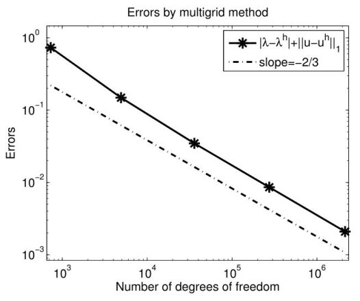
Figure 2: The errors of approximate solutions derived by Algorithm 4.2 for Example 1.

Table 1: The CPU time of Algorithm 4.2 and the direct finite element method for Example 1.

Mesh level	Number of degrees of freedom	Time of Algorithm 4.2	Time of direct FEM
1	729	0.1643	0.1643
2	4913	0.2642	1.1434
3	35937	1.1011	12.2292
4	274625	8.3957	151.3532
5	2146689	66.9435	3947.5318
6	16974593	540.2690	-

6.2 Example 2

In the second example, we use Algorithm 5.3 to solve the Gross-Pitaevskii equation (67) in $\Omega=[0,1]^{3}$, where $W=x_{1}^{2}+x_{2}^{2}+x_{3}^{2}+sin^{2}(2\pi x_{1})+sin^{2}(2\pi x_{2})+sin^{2}(2\pi x_{3})$ and $\zeta=100$.

In this example, due to the strong nonlinearity, Algorithm 4.2 does not converge. Thus, we used Algorithm 5.3 to solve the nonlinear eigenvalue problem and the convergent results are obtained.

The quadratic finite element space was adopted in this example. The sequence of meshes was produced through a one-time uniform refinement. Thus, the refinement index $\beta$ between two consecutive meshes equals $2$. The initial mesh is depicted in Figure 3.

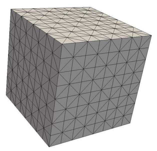
Figure 3: The initial mesh for Example 2.

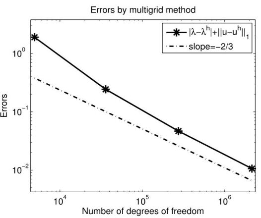
Figure 4: The errors of approximate solutions derived by Algorithm 5.3 for Example 2.

Because the exact solution of (67) is unknown, we select an adequately accurate approximation on a sufficiently fine mesh as the exact solution ($\lambda=205.112532$). The error estimates of the approximate solutions derived by Algorithm 5.3 are shown in Figure 4. The results show that Algorithm 5.3 is able to derive the approximate solutions with the optimal error estimates. In order to intuitively illustrate the efficiency of Algorithm 5.3, the computational time of Algorithm 5.3 and the direct finite element method are presented in Table 2. We can see that the linear computational complexity can be obtained with the refinement of mesh. In addition, Algorithm 5.3 has a great advantage over the direct finite element method.

In Table 3, we also present the value of $\theta_{k}$ in each finite element space $X_{h_{k}}$. The residuals corresponding to different $\theta_{k}$ are also presented. Based on the adaptive strategy, we can see that the value of the residual monotonically decreases with the refinement of mesh, and the results are consistent with Theorem 5.1.

Table 2: The CPU time of Algorithm 5.3 and the direct finite element method for Example 2.

Mesh level	Number of degrees of freedom	Time of Algorithm 5.3	Time of direct FEM
1	4913	2.1944	2.1944
2	35937	3.0003	24.5324
3	274625	10.7252	289.6608
4	2146689	80.1640	7560.2502
5	16974593	676.3930	-

Table 3: The value of $\theta_{k}$ in Algorithm 5.3 for Example 2.

Mesh level	The value of $\theta_{k}$	The value of $Resi$
1	0.5	17.8814
2	0.5	8.9953
3	0.5	4.4768
4	0.5	2.2358
5	0.5	1.1355

7 Concluding remarks

In this study, we designed a novel multigrid method to solve the nonlinear eigenvalue problem on the basis of the Newton iteration. The novel scheme transforms the nonlinear eigenvalue problem into a series of linearized boundary value problems defined in a sequence of product finite element spaces. Because of avoiding solving large-scale nonlinear eigenvalue problems directly, the overall solving efficiency is significantly improved. Besides, the optimal error estimate and linear complexity can be derived simultaneously. In addition, an improved multigrid method coupled with the mixing scheme is also introduced. The improved scheme can make the iteration scheme converge for more complicated models. More importantly, a convergence result is derived which is missing in the existing literature on the mixing scheme for nonlinear eigenvalue problems.

Declarations

Conflict of interest: The authors declare that they have no conflicts of interest/competing interests.
Code Availability: The custom codes generated during the current study are available from the corresponding author on reasonable request.

References

- (1) R. A. Adams, Sobolev Spaces, Academic Press, New York, 1975.
- (2) D. G. Anderson, Iterative procedures for nonlinear integral equations, J. Assoc. Comput. Mach., 12 (1965), 547–560.
- (3) G. Bao, G. Hu and D. Liu, An h-adaptive finite element solver for the calculations of the electronic structures, J. Comput. Phys., 231(14) (2012), 4967–4979.
- (4) W. Bao, Q. Du, Computing the ground state solution of Bose-Einstein condensates by a normalized gradient flow, SIAM J. Sci. Comput., 25 (2004), 1674–1697.
- (5) M. Benzi, G. H. Golub and J. Liesen, Numerical solution of saddle point problems, Acta Numer., 14 (2005), 1–137.
- (6) A. Brandt, Multi-level adaptive solutions to boundary-value problems, Math. Comput., 31 (1977), 333–390.
- (7) F. Brezzi and F. Fortin, Mixed and Hybrid Finite Element Methods, Springer-Verlag, New York, 1991.
- (8) S. Brenner and L. Scott, The Mathematical Theory of Finite Element Methods, Springer-Verlag, New York, 1994.
- (9) Y. Cai, L. Zhang, Z. Bai and R. Li, On an eigenvector-dependent nonlinear eigenvalue problem, SIAM J. Matrix Anal. Appl., 39(3) (2018), 1360–1382.
- (10) E. Cancès, R. Chakir and Y. Maday, Numerical analysis of nonlinear eigenvalue problems, J. Sci. Comput., 45(1-3) (2010), 90–117.
- (11) E. Cancès, R. Chakir and Y. Maday, Numerical analysis of the planewave discretization of some orbital-free and Kohn-Sham models, ESAIM Math. Model. Numer. Anal., 46 (2012), 341–388.
- (12) H. Chen, L. He and A. Zhou, Finite element approximations of nonlinear eigenvalue problems in quantum physics, Comput. Methods Appl. Mech. Engrg., 200(21) (2011), 1846–1865.
- (13) H. Chen, F. Liu and A. Zhou, A two-scale higher-order finite element discretization for Schrödinger equation, J. Comput. Math., 27 (2009), 315–337.
- (14) H. Chen, H. Xie and F. Xu, A full multigrid method for eigenvalue problems, J. Comput. Phys., 322 (2016), 747–759.
- (15) P. G. Ciarlet and J. L. Lions (eds.): Finite Element Methods, Handbook of Numerical Analysis, vol. II, North Holland, Amsterdam, 1991.
- (16) H. Fang and Y. Saad, Two classes of multisecant methods for nonlinear acceleration, Numer. Linear Algebra Appl., 16(3) (2009), 197–221.
- (17) R. P. Fedorenko, A relaxation method for solving elliptic difference equations, USSR Computational Mathematics and Mathematical Physics., 1(4) (1961), 1092–1096.
- (18) W. Hackbusch, Multi-grid Methods and Applications, Springer-Verlag, Berlin, 1985
- (19) R. Harrison, I. Moroz and K.P. Tod, A numerical study of the Schrödinger-Newton equations, Nonlinearity, 16 (2003), 101–122.
- (20) G. Hu, H. Xie and F. Xu, A multilevel correction adaptive finite element method for Kohn-Sham equation, J. Comput. Phys., 355 (2018), 436–449.
- (21) S. Jia, H. Xie, M. Xie and F. Xu, A full multigrid method for nonlinear eigenvalue problems, Sci. China Math., 59 (2016), 2037–2048.
- (22) W. Kohn and L. Sham, Self-consistent equations including exchange and correlation effects, Phys. Rev. A, 140 (1965), 1133–1138.
- (23) E. H. Lieb, Thomas-Fermi and related theories of atoms and molecules, Rev. Mod. Phys., 53 (1981), 603–641.
- (24) L. Lin and C. Yang, Elliptic preconditioner for accelerating the self-consistent field iteration in Kohn-Sham density functional theory, SIAM J. Sci. Comput., 35(5) (2013), S277–S298.
- (25) P. A. Lott, H. F. Walker, C. S. Woodward, and U. M. Yang, An accelerated Picard method for nonlinear systems related to variably saturated flow, Adv. Water Resour., 38 (2012), 92–101.
- (26) P. Motamarri, M. Iyer, J. Knap, V. Gavini, Higher-order adaptive finite-element methods for orbital-free density functional theory, J. Comput. Phys., 231 (2012), 6596–6621.
- (27) S. Pollock, L. Rebholz, and M. Xiao, Anderson-accelerated convergence of picard iterations for incompressible Navier-Stokes equations, SIAM J. Numer. Anal., 57(2) (2019), 615–637.
- (28) P. Stasiak and M.W. Matsen, Efficiency of pseudo-spectral algorithms with anderson mixing for the SCFT of periodic block-copolymer phases, Eur. Phys. J. E, 34(110) (2011), 1–9.
- (29) V. V. Shaidurov, Multigrid Methods for Finite Element, Kluwer Academic Publics, Netherlands, 1995.
- (30) A. Toth and C. T. Kelley, Convergence analysis for Anderson acceleration, SIAM J. Numer. Anal., 53(2) (2015), 805–819.
- (31) J. Xu, Iterative methods by space decomposition and subspace correction, SIAM Rev., 34 (1992), 581–613.
- (32) J. Xu and A. Zhou, A two-grid discretization scheme for eigenvalue problems, Math. Comp., 70 (2001), 17–25.
- (33) H. Yserentant, On the regularity of the electronic Schrödinger equation in Hilbert spaces of mixed derivatives, Numer. Math., 98(4) (2004), 731–759.
- (34) A. Zhou, An analysis of finite-dimensional approximations for the ground state solution of Bose-Einstein condensates, Nonlinearity, 17 (2004), 541–550.
- (35) A. Zhou, Finite dimensional approximations for the electronic ground state solution of a molecular system, Math. Methods Appl. Sci., 30 (2007), 429–447.