Non-convex Pose Graph Optimization in SLAM via Proximal Linearized Riemannian ADMM

Abstract

Pose graph optimization (PGO) is a well-known technique for solving the pose-based simultaneous localization and mapping (SLAM) problem. In this paper, we represent the rotation and translation by a unit quaternion and a three-dimensional vector, and propose a new PGO model based on the von Mises-Fisher distribution. The constraints derived from the unit quaternions are spherical manifolds, and the projection onto the constraints can be calculated by normalization. Then a proximal linearized Riemannian alternating direction method of multipliers (PieADMM) is developed to solve the proposed model, which not only has low memory requirements, but also can update the poses in parallel. Furthermore, we establish the iteration complexity of $O(1/\epsilon^{2})$ of PieADMM for finding an $\epsilon$-stationary solution of our model. The efficiency of our proposed algorithm is demonstrated by numerical experiments on two synthetic and four 3D SLAM benchmark datasets.

I Introduction

Simultaneous localization and mapping (SLAM) [1, 2] is a crucial technology that allows mobile robots to navigate autonomously through partially or fully unknown environments. It consists in the concurrent estimation of the state of a robot with on-board sensors, and the construction of the map of the environment that the sensors are detecting. SLAM can be categorized into different types based on the categories of sensors and mapping techniques, such as visual SLAM [3], laser SLAM [4], inertial SLAM [5], etc.

The classical approaches for solving the SLAM problem can be categorized as filter-based [6] or graph-based [7] methods. In the first twenty years since the SLAM problem was proposed in 1986, the filter-based methods with probabilistic formulations had achieved accurate estimation. However, updating the covariance matrix is computationally expensive in large-scale problems. The graph-based methods, first introduced in 1997 by Lu and Milios [8], were cheap with the growth of the graph. With the increase of the computational power, optimization algorithms for graph-based SLAM have received widespread attention, compared with the classical filter-based methods, such as extended Kalman filters [2], Rao–Blackwellized particle filters [9], and information filters [10]. Wilbers et al. [11] have shown the graph-based localization achieves a higher accuracy than the particle filter.

Pose graph optimization (PGO) [12, 7] can be modeled as a non-convex optimization problem underlying graph-based SLAM, in which it associates each pose with a vertex and each measurement with an edge of a graph, and needs to estimate a number of unknown poses from noisy relative measurements. The pose in 3D space typically consists of rotation and translation, where the rotation can be formulated using Euler angles, axis-angle ($so(3)$), special orthogonal group ($SO(3)$) or quaternion ($\mathbb{Q}$), and the translation is specified by a three-dimension vector $\bm{t}$. Besides, the overall pose can also be represented using special Euclidean group ($SE(3)$), Lie algebra ($se(3)$) or dual quaternion ($\mathbb{DQ}$). Different modeling methods will produce different constraints, such as no constraints in $se(3)$, matrix orthogonal and determinant constraints in $SE(3)$, or spherical constraints in $\mathbb{Q}$. Selecting a simple representation that is compatible with the problem structure will lead to an easier to solve and more accurate model.

I-A Literature Review

In the last twenty years, a lot of models have been developed in terms of the different statistical distribution of noise and representation of poses. At the same time, many efficient optimization algorithms have also been proposed to solve these models. We list several results in Table I and then give a comment.

TABLE I: Related works for solving the SLAM problem. The algorithms SGD, G-N, L-M, TRM, SDR and GPM represent stochastic gradient descent, Gauss-Newton, Levenberg–Marquardt, Trust-Region methods, semi-definite relaxation and generalized proximal methods, respectively. The “m" in algorithms indicates manifold optimization methods.

Paper	Space	Variables	Distribution	Initialization	Algorithms	Convergence	Complexity
Olson et al. [13]	2D	$SE(2)$	Gaussian	Odometry	SGD	-	-
Grisetti et al. [14]	3D	$se(3)$	Gaussian	Odometry	SGD	-	-
Dellaert and Kaess [15]	3D	$se(3)$	Gaussian	Odometry	SAM	-	-
Kaess et al. [16, 17]	3D	$se(3)$	Gaussian	Odometry	iSAM	-	-
Grisetti et al. [18]	3D	$\mathbb{AU}$	Gaussian	Odometry	mG-N	-	-
Rosen et al. [19]	3D	$se(3)$	Gaussian	Odometry	TRM	-	-
Wagner et al. [20]	3D	$SE(3)$	Gaussian	Odometry	mG-N & mL-M	-	-
Kümmerle et al. [21]	3D	$se(3)$	Gaussian	Odometry	L-M	-	-
Cheng et al. [22]	3D	$\mathbb{DQ}$	Gaussian	Odometry	G-N	-	-
Liu et al. [23]	2D	$SE(2)$	Gaussian	Odometry	SDR	-	-
Rosen et al. [24]	3D	$SE(3)$	Gaussian	Convex Relaxation	L-M	-	-
Carlone et al. [25]	3D	$SE(3)$	Gaussian+vMF	Chord	Dual method	-	-
Rosen et al. [26]	3D	$SE(3)$	Gaussian+vMF	Chord	SE-Sync	✓	-
Fan and Murphey [27]	3D	$SE(3)$	Gaussian+vMF	Chord	GPM	✓	-
This paper	3D	$\mathbb{AU}$	Gaussian+vMF	Chord	PieADMM	✓	✓

From the perspective of the models, the statistical distribution of rotational noise is typically categorized into Gaussian or isotropic von Mises-Fisher (vMF) distribution, while translational noise is uniformly characterized as Gaussian noise. Based on maximum likelihood estimator, the Gaussian noise on $se(3)$ can directly derive an unconstrained nonlinear least square model [15, 14, 17, 21]. Similarly, Cheng et al. [22] established a least square model based on unit dual quaternion, and proposed a more efficient method to compute the Jacobian matrices. By eliminating two variables, their model is also unconstrained. Another modeling method represented the rotations by $SO(3)$, which was assumed to obey the vMF distribution and derived a model with orthogonal and determinant constraints [25, 27, 26]. Since $se(3)$ needs to be transformed to describe the process of motion, the expression of the objective function modeled by $SO(3)$ or $\mathbb{Q}$ and a three-dimension vector in [25, 27, 26] is more concise compared with the unconstrained model in [15, 14, 17, 21]; however, the incorporation of constraints introduces challenges.

From the perspective of the algorithms, several efficient and accurate methods are proposed for solving large-scale problems in SLAM. The first-order optimization methods such as stochastic gradient descent [14, 13] can reduce the complexity of gradient calculation and solve the unconstrained optimization problem effectively. The algorithms with faster convergence rate, such as Gauss-Newton method [15], Levenberg–Marquardt method [21], trust-region method [19], had also been introduced to solve this problem. Instead of computing the matrix inverse, [15, 17, 16] used the matrix factorization techniques, such as QR or Cholesky factorization, to reduce the complexity, and proposed an incremental version. Grisetti et al. [18] and Wagner et al. [20] proposed the manifold-based Gauss-Newton algorithms, in which the Jacobian matrices had a sparse structure and the update process avoided the expensive storage of large-scale systems of linear equations.

However, the second-order algorithms have fast convergence rate only in the local region, and usually return a local minima for non-convex problems. Later work had focused on finding a better initial point and confirming the optimality of the solution. Rosen et al. [19] presented a robust incremental least-squares estimation based on Powell’s Dog-Leg trust-region method and improved the numerical stability. Carlone et al. [25] derived a quadratic constrained quadratic programming and verified the optimal solution by checking the dual gap. In [24], a convex relaxation is proposed by expanding the feasible set to its convex closure, which can effectively overcome the difficulty of initial point selection of non-convex problems. Furthermore, Rosen et al. [26] relaxed the model into a semidefinite program, and proved that the minimizer of its relaxation provides an exact maximum-likelihood estimate so long as the noise falls below a certain critical threshold. Fan and Murphey [27] proposed an upper bound of PGO, and solved it by the generalized proximal method which can converge to the first-order critical points and do not rely on Riemannian gradients. Another approach to find a better local minima or global minima depended on initialization techniques [12, 28]. They pointed that the non-convex rotation estimation were the actual reason why SLAM is a difficult problem, and the translations had a minor influence on the rotation estimate. Therefore, computing a good rotation estimation will improve the performance of algorithms.

I-B Contributions

In this paper, based on augmented unit quaternion [29] which uses the unit quaternions and three-dimension vectors to represent the rotations and translations, respectively, we propose a new non-convex pose graph optimization model under von Mises-Fisher distribution [30]:

$$\underset{\{\tilde{q}_{i}\},\{\bm{t}_{i}\}}{\min} ~{}~{}\sum_{(i,j)\in\mathcal{E}}\|\tilde{t}_{j}-\tilde{t}_{i}-\tilde{q}_{i}\tilde{t}_{ij}\tilde{q}_{i}^{*}\|_{\Sigma_{1}}^{2}+\|\tilde{q}_{j}^{*}\tilde{q}_{i}\tilde{q}_{ij}-1\|_{\Sigma_{2}}^{2},$$

$$\operatorname{s.t.}{}{} \quad\tilde{q}_{i}\in\mathbb{U},~{}\bm{t}_{i}\in\mathbb{R}^{3},~{}i=1,2,\dots,n.$$

Here, the constraint $\mathbb{U}$ is a unit sphere. Compared with the special orthogonal group constraints, the projection of unit quaternions can be calculated by simple normalization without singular value decomposition. In addition, since a unit quaternion in $\mathbb{U}$ requires storing four elements in the computation process, while a rotation matrix in $SO(3)$ requires storing nine elements, the quaternion representation has lower data storage. The established model constitutes a nonlinear least square problem with a quartic objective function. The non-convex structures and spherical manifold constraints may make the model difficult to solve. By introducing redundant variables, it can be reformulated into a multi-linear least square problem:

$$\underset{\{\tilde{p}_{i}\},\{\tilde{q}_{i}\},\{\bm{t}_{i}\}}{\min} \sum_{(i,j)\in\mathcal{E}}\|\tilde{t}_{j}-\tilde{t}_{i}-\tilde{q}_{i}\tilde{t}_{ij}\tilde{p}_{i}^{*}\|_{\Sigma_{1}}^{2}+\|\tilde{p}_{j}^{*}\tilde{q}_{i}\tilde{q}_{ij}-1\|_{\Sigma_{2}}^{2},$$

$$\operatorname{s.t.}{}{}{}{} \tilde{p}_{i}=\tilde{q}_{i},~{}\tilde{p}_{i}\in\mathbb{U},~{}\tilde{q}_{i}\in\mathbb{R}^{4},~{}\bm{t}_{i}\in\mathbb{R}^{3},~{}i=1,\dots,n.$$

The variables $\tilde{p}_{i}$ and $\tilde{q}_{i}$ in the objective function are coupled, while each individual variable retains linearity and convexity. One valid method for solving this category of problems is splitting algorithms [31, 32], and they have been proven effective in fields such as compressive sensing, robust principal component analysis and tensor decomposition.

We propose a proximal linearized Riemannian alternating direction method of multipliers (PieADMM) for the non-convex pose graph optimization, which updates the other variables using the most recent partial information. Our subproblems not only have closed-form solutions, but also can be computed in parallel, which results in a low time complexity per update. The above superiority is verified in the large-scale numerical experiments. Theoretically, the convergence analysis is established to complement our findings.

Now we summarize our contributions in this paper as follows:

1. We propose a non-convex pose graph optimization model based on augmented unit quaternion and vMF distribution, in which the data storage is low-cost and the projection of unit quaternions can be calculated by normalization.

2. We propose a PieADMM which has closed-form solutions in its subproblems, and update them in parallel.

3. Based on the first-order optimality conditions on manifolds, we define an $\epsilon$-stationary solution of our model. Then, we establish the iteration complexity of $O(1/\epsilon^{2})$ of PieADMM for finding an $\epsilon$-stationary solution.

4. We test our algorithm on two synthetic datasets with different data scales and four 3D SLAM benchmark datasets. Numerical experiments verify the effectiveness of our method.

The remaining parts of this paper are organized as follows. In the next section, we review some basic properties of quaternions and Riemannian submanifolds. In Sect. III, we present an augmented unit quaternion model which is constrained on the sphere manifolds. The PieADMM is proposed in Sect. IV. In Sect. V, we establish the iteration complexity of $O(1/\epsilon^{2})$ of PieADMM for finding an $\epsilon$-stationary solution. Finally, in Sect. VI, we present the numerical results.

II Notation and preliminaries

In this section, we introduce some basic notations, definitions and lemmas for this paper.

The fields of real numbers, quaternion numbers and unit quaternion numbers are denoted by $\mathbb{R}$, $\mathbb{Q}$ and $\mathbb{U}$, respectively. Throughout this paper, scalars, vectors, matrices, and quaternions are denoted by lowercase letters (e.g., $x$), boldface lowercase letters (e.g., $\bm{x}$), boldface capital letters (e.g., $X$), and lowercase letters with tilde (e.g., $\tilde{x}$), respectively. The special orthogonal group $SO(3)$ is the set of three-dimensional rotations which is formally defined by $SO(3):=\{R\in\mathbb{R}^{3\times 3}\mid R^{\top}R=I_{3},\operatorname{det}(R)=1\}$, and the special Euclidean group is the set of poses defined by $SE(3)\triangleq\{(R,\bm{t}):R\in SO(3),\bm{t}\in\mathbb{R}^{3}\}$.

The notation $\left\|\cdot\right\|$ denotes the $2$-norm of vectors or the Frobenius norm of matrices. Let $M$ be a positive definite linear operator; we use $\|\bm{x}\|_{M}:=\sqrt{\left\langle\bm{x},M\bm{x}\right\rangle}$ to denote its $M$-norm; and $\sigma_{\min}(M)$ and $\sigma_{\max}(M)$ denote the smallest and largest eigenvalue of $M$, respectively. For symmetric matrices $M_{1},M_{2}\in\mathbb{R}^{n\times n}$, $M_{1}\succ M_{2}$ and $M_{1}\succeq M_{2}$ means that $M_{1}-M_{2}$ is positive definite and positive semidefinite, respectively.

The followings are some preliminaries about quaternions (Section II-A) and ADMM (Section II-B), respectively.

II-A Quaternion and pose

A quaternion number $\tilde{q}\in\mathbb{Q}$, proposed by Hamilton, has the form $\tilde{q}=q_{0}+q_{1}\mathbf{i}+q_{2}\mathbf{j}+q_{3}\mathbf{k}$, where $q_{0},q_{1},q_{2},q_{3}\in\mathbb{R}$ and $\mathbf{i},\mathbf{j},\mathbf{k}$ are three imaginary units. We may also write $\tilde{q}=[q_{0},q_{1},q_{2},q_{3}]=[q_{0},\bm{q}]\in\mathbb{R}^{4}$ as the vector representation where $\bm{q}=[q_{1},q_{2},q_{3}]\in\mathbb{R}^{3}$ for convenience. We note that we also regard the above representation as a column vector and its transpose $[q_{0},\bm{q}]^{\top}$ a row vector. The sum of $\tilde{p}$ and $\tilde{q}$ is defined as $\tilde{p}+\tilde{q}=[p_{0}+q_{0},\bm{p}+\bm{q}].$ The product of $\tilde{p}$ and $\tilde{q}$ is defined by

$$\tilde{p}\tilde{q}=\left[p_{0}q_{0}-\bm{p}\cdot\bm{q},p_{0}\bm{q}+q_{0}\bm{p}+\bm{p}\times\bm{q}\right],$$

where $\bm{p}\cdot\bm{q}$ is the $\operatorname{dot}$ product, and $\bm{p}\times\bm{q}$ is the cross product of $\bm{p}$ and $\bm{q}$. Thus, in general, $\tilde{p}\tilde{q}\neq\tilde{q}\tilde{p}$, and we have $\tilde{p}\tilde{q}=\tilde{q}\tilde{p}$ if and only if $\bm{p}\times\bm{q}=\vec{0}$, i.e., either $\bm{p}=\vec{0}$ or $\bm{q}=\vec{0}$, or $\bm{p}=\alpha\bm{q}$ for some real number $\alpha$ (see [29]). The multiplication of quaternions is associative and distributive over vector addition, but is not commutative.

The conjugate of $\tilde{q}$ is the quaternion $\tilde{q}^{*}=q_{0}-q_{1}\mathbf{i}-q_{2}\mathbf{j}-q_{3}\mathbf{k}$. Then, $(\tilde{p}\tilde{q})^{*}=\tilde{q}^{*}\tilde{p}^{*}$ for any $\tilde{p},\tilde{q}\in\mathbb{Q}$. The magnitude of $\tilde{q}$ is defined by $\|\tilde{q}\|=\sqrt{\tilde{q}\tilde{q}^{*}}=\sqrt{\tilde{q}^{*}\tilde{q}}.$ And $\tilde{q}$ is invertible if and only if $\|\tilde{q}\|$ is positive. In this case, we have $\tilde{q}^{-1}=\tilde{q}^{*}/\|\tilde{q}\|.$

The quaternion $\tilde{q}\in\mathbb{Q}$ is called a unit quaternion if

$$\|\tilde{q}\|=\sqrt{q_{0}^{2}+q_{1}^{2}+q_{2}^{2}+q_{3}^{2}}=1.$$

Denote the set of all unit quaternions by $\mathbb{U}$, which can be regarded as a unit sphere in $\mathbb{R}^{4}$. Equivalently, a unit quaternion has the following form:

$$\tilde{q}=[\cos(\theta/2),\sin(\theta/2)\bm{n}],$$

where $\bm{n}=(n_{x},n_{y},n_{z})$ is a unit vector and $\theta$ is an angle. Then, we will show that $\theta\bm{n}\in so(3)$, $\tilde{q}\in\mathbb{U}$ and $R\in SO(3)$ can all represent rotation and realize motion . Let a vector $\bm{t}_{1}\in\mathbb{R}^{3}$ rotates $\theta$ radians around axis $\bm{n}$ to reach $\bm{t}_{2}\in\mathbb{R}^{3}$. This process can be represented by quaternion as

$$[0,\bm{t}_{2}]=\tilde{q}[0,\bm{t}_{1}]\tilde{q}^{*}.$$

Using rotation matrix in $SO(3)$, we also have $\bm{t}_{2}=R\bm{t}_{1}$, where

$$R=\cos(\theta)I_{3}+(1-\cos(\theta))\bm{n}\bm{n}^{\top}+\sin(\theta)\bm{n}^{\land},$$

and

$$\bm{n}^{\land}=\left(\begin{array}[]{ccc}0&-n_{z}&n_{y}\\ n_{z}&0&-n_{x}\\ -n_{y}&n_{x}&0\end{array}\right).$$

The relationship between rotation matrix and unit quaternion is given in the next lemma.

Lemma II.1

[33] Given a unit quaternion $\tilde{q}=[q_{0},\bm{q}]=[q_{0},q_{1},q_{2},q_{3}]\in\mathbb{U}$ and a vector $\bm{t}\in\mathbb{R}^{3}$. Then $[0,R\bm{t}]=\tilde{q}[0,\bm{t}]\tilde{q}^{*}$, where the rotation matrix $R\in SO(3)$ satisfies

$$R=\bm{q}\bm{q}^{\top}+q_{0}^{2}I+2q_{0}\bm{q}^{\land}+(\bm{q}^{\land})^{2}.$$

If the rotation matrix $R$ is compound motion of two rotations, i.e., $R=R_{2}R_{1}$, then the corresponding quaternion $\tilde{q}$ can be formulated as $\tilde{q}=\tilde{q}_{2}\tilde{q}_{1}$. Next, we show a lemma which can simplify the product of two quaternions by multiplication between matrix and vector. Given any $\tilde{a}=[a_{0},a_{1},a_{2},a_{3}]$, we define

$$M(\tilde{a})=\left(\begin{array}[]{rrrr}a_{0}&-a_{1}&-a_{2}&-a_{3}\\ a_{1}&a_{0}&-a_{3}&a_{2}\\ a_{2}&a_{3}&a_{0}&-a_{1}\\ a_{3}&-a_{2}&a_{1}&a_{0}\end{array}\right),$$

and

$$W(\tilde{a})=\left(\begin{array}[]{rrrr}a_{0}&-a_{1}&-a_{2}&-a_{3}\\ a_{1}&a_{0}&a_{3}&-a_{2}\\ a_{2}&-a_{3}&a_{0}&a_{1}\\ a_{3}&a_{2}&-a_{1}&a_{0}\end{array}\right).$$

Lemma II.2

[34] For any $\tilde{a}=[a_{0},a_{1},a_{2},a_{3}]\in\mathbb{Q}$ and $\tilde{b}=[b_{0},b_{1},b_{2},b_{3}]\in\mathbb{Q}$, the following statements hold

1. $M(\tilde{a}^{*})=M(\tilde{a})^{\top}$, $W(\tilde{a}^{*})=W(\tilde{a})^{\top}$.

2. $\tilde{a}\tilde{b}=M(\tilde{a})\tilde{b}=W(\tilde{b})\tilde{a}$.

3. $M(\tilde{a})^{\top}M(\tilde{a})=W(\tilde{a})^{\top}W(\tilde{a})=\|\tilde{a}\|^{2}I_{4}$, where $I_{4}$ is the identity matrix of size $4\times 4$.

A quaternion $\tilde{q}=[0,q_{1},q_{2},q_{3}]\in\mathbb{Q}$ is called a vector quaternion which has the following properties.

Lemma II.3

[29] Given a quaternion $\tilde{q}\in\mathbb{Q}$, the following statements hold

1. $\tilde{q}$ is a vector quaternion if and only if $\tilde{q}=-\tilde{q}^{*}$.

2. if $\tilde{q}$ is a vector quaternion, then $\tilde{p}\tilde{q}\tilde{p}^{*}$ is still a vector quaternion for any quaternion $\tilde{p}\in\mathbb{Q}$.

Following [29], we denote $\mathbb{AU}\triangleq\{(\tilde{q},\bm{t}):\tilde{q}\in\mathbb{U},\bm{t}\in\mathbb{R}^{3}\}$ as augmented unit quaternions. An augmented unit quaternion vector $(\tilde{\bm{p}},\bm{t})=(\tilde{p}_{1},\bm{t_{1}},\tilde{p}_{2},\bm{t_{2}},\dots,\tilde{p}_{n},\bm{t_{n}})\in\mathbb{AU}^{n}$ is an $n$-component vector, such that each component $(\tilde{p}_{i},\bm{t_{i}})$ is an augmented unit quaternion. In fact, $\mathbb{AU}^{n}$ is consist of the Cartesian product of $n$ spheres and $3n$-dimensional Euclidean space $\mathbb{R}^{3n}$, which is embedded in Euclidean space $\mathbb{R}^{7n}$. As will be mentioned in the “Appendix A", the set $\mathbb{AU}^{n}$ is a Riemannian submanifold. An augmented unit quaternion optimization problem can be formulated as

$$\min f(\tilde{\bm{p}},\bm{t})\quad\text{s.t.}~{}(\tilde{\bm{p}},\bm{t})\in\mathbb{AU}^{n},$$

which is also a $7n$-dimensional equality constrained optimization problem, with $7n$ real variables and $n$ spherical equality constraints.

II-B Alternating direction method of multipliers

Alternating direction method of multipliers (ADMM) is an effective splitting algorithm for solving large-scale problems, which has been applied in many fields, such as the image alignment problem [35], the robust principal component analysis model [36], phase retrieval [37] and background/foreground extraction problem [38]. The classical ADMM is proposed by Glowinski and Marrocco [39] and Gabay and Mercier [40] for solving the linearly constrained convex optimization problem with two blocks of variables:

$$\underset{x_{1},x_{2}}{\min}{} \quad\theta_{1}(x_{1})+\theta_{2}(x_{2})$$

$$\operatorname{s.t.}{} \quad A_{1}x_{1}+A_{2}x_{2}=b,\quad x_{i}\in\mathcal{X}_{i},~{}i=1,2.$$

The corresponding iteration scheme of ADMM is

$$\left\{\begin{aligned} x_{1}^{k+1}&=\arg\min\left\{\mathcal{L}_{\beta}\left(x_{1},x_{2}^{k},z^{k}\right)\mid x_{1}\in\mathcal{X}_{1}\right\},\\ x_{2}^{k+1}&=\arg\min\left\{\mathcal{L}_{\beta}\left(x_{1}^{k+1},x_{2},z^{k}\right)\mid x_{2}\in\mathcal{X}_{2}\right\},\\ z^{k+1}&=z^{k}-\beta\left(A_{1}x_{1}^{k+1}+A_{2}x_{2}^{k+1}-b\right),\end{aligned}\right.$$

where

$$\mathcal{L}_{\beta}(x_{1},x_{2},z)= \theta_{1}(x_{1})+\theta_{2}(x_{2})-\left\langle z,A_{1}x_{1}+A_{2}x_{2}-b\right\rangle$$

$$+\frac{\beta}{2}\|A_{1}x_{1}+A_{2}x_{2}-b\|^{2}.$$

The variable $z$ is the Lagrange multiplier and $\beta>0$ is a penalty parameter. It could be proved to converge to a solution globally under some mild conditions and achieve linear rate of convergence [41]. Furthermore, ADMM had also been extended to multi-block [42, 43, 44] and non-convex [45, 46] cases:

$$\underset{x_{1},x_{2},\dots,x_{n}}{\min}{} ~{}\sum_{i=1}^{n}\theta_{i}(x_{i})$$

$$\operatorname{s.t.}{} ~{}\sum_{i=1}^{n}A_{i}x_{i}=b,\quad x_{i}\in\mathcal{X}_{i},~{}i=1,2,\dots,n.$$

The convergence for multi-block case is not guaranteed even for convex problems [43]. There are two ways in guaranteeing convergence of ADMM-type method for solving multi-block optimization problems, one is to twist the point generated by classical scheme, and the other one is to assume further conditions on the functions or the matrices [32]. Hong et al. [47] discussed the linearly constrained consensus and sharing problems which had the following nonseparable structure:

$$\underset{x_{1},x_{2},\dots,x_{n}}{\min}{} ~{}H(x_{1},x_{2},\dots,x_{n})+\sum_{i=1}^{n}\theta_{i}(x_{i})$$

$$\operatorname{s.t.}{} ~{}\sum_{i=1}^{n}A_{i}x_{i}=b,\quad x_{i}\in\mathcal{X}_{i},~{}i=1,2,\dots,n.$$

Although the variables in $H(\cdot)$ were coupled, the experiment results shown that ADMM still had a good performance when the subproblems had closed-form solutions. In theory, the iterative sequence can converge to a critical point of the augmented Lagrangian function. We refer readers to [48, 49] for more details.

In recent years, some scholars have devoted themselves to multi-block linear equality constrained problem with Riemannian submanifold constraints. There is no guarantee that the manifold constraints can be strictly satisfied for the traditional methods in Euclidean space. In this case, it is usually necessary to project the last iteration point on the constraint sets. However, the manifold optimization algorithm can ensure the feasibility of the iterative sequence on the manifold. Zhang et al. [50] considered the gradient-based Riemannian ADMM and gave an iteration complexity. Li et al.[51] discussed the nonsmoooth problem solving by Moreau envelope smoothing technique. In general, the research about Riemannian ADMM is still at an early stage.

III The Augmented Unit Quaternion Model

In this section, we propose a new PGO model based on augmented unit quaternions. The traditional PGO models represent the unknown poses and the measurements in $SE(3)$ or $se(3)$. Instead of orthogonal rotation matrix $SO(3)$ or aixs-angle representation $so(3)$, we use unit quaternions in $\mathbb{U}$ to represent rotations, which is a simple spherical manifold and can be solved efficiently by proximal operators.

PGO can be visualized as a directed graph $\mathcal{G}=(\mathcal{V},\mathcal{E})$, see [25, 24, 14], in which each vertex $i\in\mathcal{V}$ corresponds to a robot pose $(\tilde{q}_{i},\bm{t}_{i})\in\mathbb{AU}$, and each directed edge $(i,j)\in\mathcal{E}$ corresponds to a relative measurement $(\tilde{q}_{ij},\bm{t}_{ij})\in\mathbb{AU}$. We define $n=|\mathcal{V}|$ and $m=|\mathcal{E}|$ which indicate the number of vertices and edges, respectively. The goal is to estimate the unknown poses from the noisy measurements. Now, we assume the following generative model for the relative pose measurements:

$$\bm{t}_{ij} =R_{i}^{\top}(\bm{t}_{j}-\bm{t}_{i})+\bm{t}_{\epsilon},\quad\text{where}~{}\bm{t}_{\epsilon}\sim~{}\mathcal{N}(0,\Omega_{1})$$

$$\tilde{q}_{ij} =\tilde{q}_{i}^{*}\tilde{q}_{j}\tilde{q}_{\epsilon},\quad\quad\quad\quad\quad~{}\text{where}~{}\tilde{q}_{\epsilon}\sim~{}\text{vMF}([1,0,0,0],\kappa)$$

where $R_{i}$ and $\tilde{q}_{i}$ are the rotation representation of vertex $i$ in $SO(3)$ and unit quaternion, respectively. “$\mathcal{N}(\bm{\mu},\Omega)$” denotes a Gaussian distribution with mean $\bm{\mu}$ and covariance matrix $\Omega$. “$\text{vMF}(\bm{\mu},\kappa)$” denotes a $d$-dimensional von Mises-Fisher distribution where $\bm{\mu}\in\mathbb{S}^{d-1}$ and $\kappa\geq 0$ are mean direction and concentration parameters, respectively. It is one of the most commonly used distributions to model data distributed on the surface of the unit hypersphere [52, 30, 53] and can be considered a circular analogue of the normal distribution. Its probability density function is given by

$$p(\bm{x};\bm{\mu},\kappa)=c_{d}(\kappa)e^{\kappa\bm{\mu}^{\top}\bm{x}}$$

where $\bm{x}\in\mathbb{S}^{d-1}$ is a $d$-dimensional unit vector, and the normalizing constant $c_{d}(\kappa)$ has the form

$$c_{d}(\kappa)=\frac{\kappa^{d/2-1}}{(2\pi)^{d/2}I_{d/2-1}(\kappa)}$$

where $I_{r}(\cdot)$ is the modified Bessel function of the first kind of order $r$. In fact, as the concentration parameter $\kappa$ increases, the vMF distribution becomes increasingly concentrated at the mean direction $\bm{\mu}$. When $\kappa=0$, it corresponds to the uniform distribution on $\mathbb{S}^{d-1}$. When $\kappa\rightarrow+\infty$, the distribution approximates to a Gaussian distribution with mean $\bm{\mu}$ and covariance $1/\kappa$. We show the von Mises-Fisher distribution in Fig. 1.

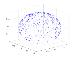
(a) $\kappa=1$

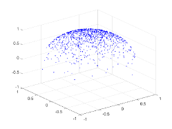
(b) $\kappa=5$

(c) $\kappa=20$

Figure 1: The illustration of the von Mises-Fisher distribution with $\bm{\mu}=[0,0,1]^{\top}$ and $\kappa=1,~{}5,~{}20$, respectively.

The parameter $d$ is the spatial dimension. In the case $d=2$, the von Mises-Fisher distribution degenerates to the von Mises distribution. And when $d=3$, it is called the Fisher distribution. We set $d=4$ which is corresponding to the unit quaternion. Then, we can build our model by the maximum likelihood estimator (MLE) or minimizing the negative log-likelihood:

$$\underset{\{\tilde{q}_{i}\}\in\mathbb{U},\{\bm{t}_{i}\}\in\mathbb{R}^{3}}{\min}\sum_{(i,j)\in\mathcal{E}}-\log l(\tilde{q}_{ij})-\log l(\bm{t}_{ij}),$$

where $l(\tilde{q}_{ij})$ and $l(\bm{t}_{ij})$ are likelihood functions defined by:

$$l(\tilde{q}_{ij}) =c_{4}(\kappa)\exp(\kappa\left\langle[1,0,0,0],\tilde{q}_{j}^{*}\tilde{q}_{i}\tilde{q}_{ij}\right\rangle),$$

$$l(\bm{t}_{ij}) =\frac{1}{(2\pi)^{3/2}|\Omega_{1}|^{1/2}}\exp\left(-\frac{1}{2}\|\bm{t}_{ij}-R_{i}^{\top}(\bm{t}_{j}-\bm{t}_{i})\|_{\Omega_{1}^{-1}}^{2}\right),$$

respectively. The negative log-likelihood for $\bm{t}_{ij}$ with Gaussian distributions is

$$-\log l(\bm{t}_{ij})=\frac{1}{2}\|\bm{t}_{ij}-R_{i}^{\top}(\bm{t}_{j}-\bm{t}_{i})\|_{\Omega_{1}^{-1}}^{2}+const,$$

where $\|\bm{x}\|_{\Omega}^{2}=\bm{x}^{\top}\Omega\bm{x}$. The negative log-likelihood for $\tilde{q}_{ij}$ with vMF distributions is

$$-\log l(\tilde{q}_{ij}) =-\kappa\left\langle[1,0,0,0],\tilde{q}_{\epsilon}\right\rangle+const$$

$$=-\kappa\left\langle[1,0,0,0],\tilde{q}_{j}^{*}\tilde{q}_{i}\tilde{q}_{ij}\right\rangle+const$$

$$=\frac{\kappa}{2}\|\tilde{q}_{j}^{*}\tilde{q}_{i}\tilde{q}_{ij}-1\|^{2}+const,$$

where the last equality follows from the fact that $\tilde{q}_{j}^{*}\tilde{q}_{i}\tilde{q}_{ij}$ is still a unit quaternion.

Based on the assumptions of noise and Lemma II.1, we can get the following optimization problem:

$$\underset{\{\tilde{q}_{i}\},\{\bm{t}_{i}\}}{\min} ~{}\sum_{(i,j)\in\mathcal{E}}\|\tilde{t}_{j}-\tilde{t}_{i}-\tilde{q}_{i}\tilde{t}_{ij}\tilde{q}_{i}^{*}\|_{\Omega_{2}}^{2}+\|\tilde{q}_{j}^{*}\tilde{q}_{i}\tilde{q}_{ij}-1\|_{\kappa I_{4}}^{2},$$

$$\operatorname{s.t.}{}{} ~{}\tilde{q}_{i}\in\mathbb{U},~{}\bm{t}_{i}\in\mathbb{R}^{3},~{}i=1,2,\dots,n,$$

where $\Omega_{2}=\left(\begin{array}[]{cc}c&0\\ 0&\Omega_{1}^{-1}\end{array}\right)$, and $c>0$ is an arbitrary scalar. By generalizing the covariance matrix $\Omega_{1}$ and concentration parameters $\kappa$, we propose our PGO model in the following:

$$\underset{\{\tilde{q}_{i}\},\{\bm{t}_{i}\}}{\min}~{}\sum_{(i,j)\in\mathcal{E}}\|\tilde{t}_{j}-\tilde{t}_{i}-\tilde{q}_{i}\tilde{t}_{ij}\tilde{q}_{i}^{*}\|_{\Sigma_{1}}^{2}+\|\tilde{q}_{j}^{*}\tilde{q}_{i}\tilde{q}_{ij}-1\|_{\Sigma_{2}}^{2},$$

$$\operatorname{s.t.}~{}~{}~{}\tilde{q}_{i}\in\mathbb{U},~{}\bm{t}_{i}\in\mathbb{R}^{3},~{}i=1,2,\dots,n,$$ (1)

where $\Sigma_{1}$, $\Sigma_{2}\in\mathcal{S}_{+}^{n}$ are positive semi-definite matrices. $\tilde{t}_{i}=[0,\bm{t}_{i}]$ is a pure quaternion. The model (1) is an unconstrained quartic polynomial optimization problem on manifold. With the development of manifold optimization, many algorithms with convergence guarantees can deal with the model (1), such as proximal Riemannian gradient method [54], Riemannian conjugate gradient method [55], and Riemannian Newton method [56]. We refer the readers to [57] for more details.

By exploiting the structure of model (1), we focus on the splitting method, whose subproblems are usually easier to solve. With respect to the variable $\bm{t}_{i}$, model (1) constitutes a quadratic optimization problem for which an explicit solution can be directly computed. With respect to variable $\tilde{q}_{i}$, the optimization problem is quartic, which may make the model difficult to solve. By introducing auxiliary variables $\tilde{p}_{i}$, $i=1,\dots,n$, we can get an equivalent model of (1):

$$\underset{\{\tilde{p}_{i}\},\{\tilde{q}_{i}\},\{\bm{t}_{i}\}}{\min} ~{}\sum_{(i,j)\in\mathcal{E}}\|\tilde{t}_{j}-\tilde{t}_{i}-\tilde{q}_{i}\tilde{t}_{ij}\tilde{p}_{i}^{*}\|_{\Sigma_{1}}^{2}+\|\tilde{p}_{j}^{*}\tilde{q}_{i}\tilde{q}_{ij}-1\|_{\Sigma_{2}}^{2},$$ (2)

$$\operatorname{s.t.}{} \tilde{p}_{i}=\tilde{q}_{i},~{}\tilde{p}_{i}\in\mathbb{U},~{}\tilde{q}_{i}\in\mathbb{R}^{4},~{}\bm{t}_{i}\in\mathbb{R}^{3},~{}i=1,\dots,n.$$

When considering the variables separately, the model (2) is reformulated to a multi-linear least square problem, whose subproblems are easier to solve than that of the nonlinear least square problem (1). The variables $\tilde{p}_{i}$ and $\tilde{q}_{i}$ in the objective function are coupled, while each individual variable retains linearity and convexity. Using the alternating update strategy, it can be seen in the next section that the subproblems have closed-form solutions, and can also be solved in parallel corresponding to the structure of the directed graph $\mathcal{E}$, which will greatly improve the algorithm efficiency.

IV Proximal Linearized Riemannian ADMM

In this section, we propose a proximal linearized Riemannian ADMM algorithm to solve PGO model (2).

Let $\tilde{\bm{p}}=(\tilde{p}_{1},\tilde{p}_{2},\dots,\tilde{p}_{n})\in\mathbb{U}^{n}$, $\tilde{\bm{q}}=(\tilde{q}_{1},\tilde{q}_{2},\dots,\tilde{q}_{n})\in\mathbb{R}^{4n}$, and $\bm{t}=(\bm{t}_{1},\bm{t}_{2},\dots,\bm{t}_{n})\in\mathbb{R}^{3n}$, where $\mathbb{U}^{n}$ represents the Cartesian product of $n$ unit quaternion sets. We define

$$f(\tilde{\bm{p}},\tilde{\bm{q}},\bm{t}) =\sum_{(i,j)\in\mathcal{E}}\|\tilde{t}_{j}-\tilde{t}_{i}-\tilde{q}_{i}\tilde{t}_{ij}\tilde{p}_{i}^{*}\|_{\Sigma_{1}}^{2},$$ (3)

$$g(\tilde{\bm{p}},\tilde{\bm{q}}) =\sum_{(i,j)\in\mathcal{E}}\|\tilde{p}_{j}^{*}\tilde{q}_{i}\tilde{q}_{ij}-1\|_{\Sigma_{2}}^{2}.$$ (4)

Then the augmented Lagrangian function of PGO model (2) is

$$\mathcal{L}_{\beta}(\tilde{\bm{p}},\tilde{\bm{q}},\bm{t},\bm{\lambda}) =f(\tilde{\bm{p}},\tilde{\bm{q}},\bm{t})+g(\tilde{\bm{p}},\tilde{\bm{q}})$$ (5)

$$+ \sum_{i=1}^{n}\left\{\delta_{\mathbb{U}}(\tilde{p}_{i})-\left\langle\bm{\lambda}_{i},\tilde{p}_{i}-\tilde{q}_{i}\right\rangle+\frac{\beta}{2}\|\tilde{p}_{i}-\tilde{q}_{i}\|^{2}\right\},$$

where $\bm{\lambda}\in\mathbb{R}^{4n}$ is the Lagrange multiplier and $\beta>0$ is a penalty parameter. The function $\delta_{\mathbb{U}}(\cdot)$ is the indicator function of $\mathbb{U}$ which is defined as

$$\delta_{\mathbb{U}}(\tilde{p}):=\left\{\begin{aligned} &0,\qquad\text{if}~{}\tilde{p}\in\mathbb{U},\\ &+\infty,~{}\text{otherwise}.\end{aligned}\right.$$

The iterative scheme of classical ADMM is given by

$$\tilde{\bm{p}}^{k+1}=\mathop{\arg\min}\limits_{\tilde{\bm{p}}\in\mathbb{U}^{n}}\mathcal{L}_{\beta}(\tilde{\bm{p}},\tilde{\bm{q}}^{k},\bm{t}^{k},\bm{\lambda}^{k}),$$ (6a)

$$\tilde{\bm{q}}^{k+1}=\mathop{\arg\min}\limits_{\tilde{\bm{q}}}\mathcal{L}_{\beta}(\tilde{\bm{p}}^{k+1},\tilde{\bm{q}},\bm{t}^{k},\bm{\lambda}^{k}),$$ (6b)

$$\bm{t}^{k+1}=\mathop{\arg\min}\limits_{\bm{t}}\mathcal{L}_{\beta}(\tilde{\bm{p}}^{k+1},\tilde{\bm{q}}^{k+1},\bm{t},\bm{\lambda}^{k}),$$ (6c)

$$\bm{\lambda}^{k+1}=\bm{\lambda}^{k}-\beta(\tilde{\bm{p}}^{k+1}-\tilde{\bm{q}}^{k+1}).$$ (6d)

In the above algorithm, the optimization subproblem (6b) and (6c) can be solved efficiently. However, because of the manifold constraints, there is no closed-form solution for (6a).

The linearized technique can help us overcome this difficulty and get a closed-form solution. In [58, 59], the authors linearized the whole augmented Lagrangian function and obtained easier subproblems. However, this may result in the slow convergence. Instead, we only use the linearization of $f$ and $g$, and keep the quadratic term $\|\tilde{p}_{i}-\tilde{q}_{i}\|^{2}$. Consequently, the linearized augmented Lagrangian function about $\tilde{\bm{p}}$ is defined as

$$\mathcal{L}_{\beta}^{k}(\tilde{\bm{p}},\tilde{\bm{q}}^{k}, \bm{t}^{k},\bm{\lambda}^{k})\!=\!f(\tilde{\bm{p}}^{k},\tilde{\bm{q}}^{k},\bm{t}^{k})\!+\!\left\langle\nabla_{\tilde{\bm{p}}}f(\tilde{\bm{p}}^{k},\tilde{\bm{q}}^{k},\bm{t}^{k}),\tilde{\bm{p}}\!-\!\tilde{\bm{p}}^{k}\right\rangle$$

$$+ g(\tilde{\bm{p}}^{k},\tilde{\bm{q}}^{k})+\left\langle\nabla_{\tilde{\bm{p}}}g(\tilde{\bm{p}}^{k},\tilde{\bm{q}}^{k}),\tilde{\bm{p}}-\tilde{\bm{p}}^{k}\right\rangle$$

$$+ \sum_{i=1}^{n}\left\{\delta_{\mathbb{U}}(\tilde{p}_{i})\!-\!\left\langle\bm{\lambda}_{i}^{k},\tilde{p}_{i}\!-\!\tilde{q}_{i}^{k}\right\rangle\!+\!\frac{\beta}{2}\|\tilde{p}_{i}\!-\!\tilde{q}_{i}^{k}\|^{2}\right\}.$$ (7)

Furthermore, an extra proximal term [60] not only can guarantee the uniqueness of the solution, but also provide a quantifiable descending of augmented Lagrangian function, which will help us analyze the convergence.

Finally, the iterative scheme of proximal linearized ADMM is given by

$$\tilde{\bm{p}}^{k+1}=\mathop{\arg\min}\limits_{\tilde{\bm{p}}\in\mathbb{U}^{n}}\mathcal{L}_{\beta}^{k}(\tilde{\bm{p}},\tilde{\bm{q}}^{k},\bm{t}^{k},\bm{\lambda}^{k})\!+\!\frac{1}{2}\|\tilde{\bm{p}}-\tilde{\bm{p}}^{k}\|_{H_{1}}^{2},$$ (8a)

$$\tilde{\bm{q}}^{k+1}=\mathop{\arg\min}\limits_{\tilde{\bm{q}}}\mathcal{L}_{\beta}(\tilde{\bm{p}}^{k+1},\tilde{\bm{q}},\bm{t}^{k},\bm{\lambda}^{k})\!+\!\frac{1}{2}\|\tilde{\bm{q}}-\tilde{\bm{q}}^{k}\|_{H_{2}}^{2},$$ (8b)

$$\bm{t}^{k+1}=\mathop{\arg\min}\limits_{\bm{t}}\mathcal{L}_{\beta}(\tilde{\bm{p}}^{k+1},\tilde{\bm{q}}^{k+1},\bm{t},\bm{\lambda}^{k})\!+\!\frac{1}{2}\|\bm{t}-\bm{t}^{k}\|_{H_{3}}^{2},$$ (8c)

$$\bm{\lambda}^{k+1}=\bm{\lambda}^{k}-\beta(\tilde{\bm{p}}^{k+1}-\tilde{\bm{q}}^{k+1}),$$ (8d)

where $H_{1}$, $H_{2}$, $H_{3}\succ 0$ are positive definite matrices with block diagonal structures. Here, $\frac{1}{2}\|\tilde{\bm{p}}-\tilde{\bm{p}}^{k}\|_{H_{1}}^{2}$ can be split as $\frac{1}{2}\sum_{i=1}^{n}\|\tilde{p}_{i}-\tilde{p}_{i}^{k}\|_{H_{1,i}}^{2}$. In other words, each block of $H_{1}$ is still a diagonal matrix with the form $H_{1,i}=\tau_{1,i}I_{4}$. We assume $H_{2}$ has similar structures.

IV-A Subproblems

In this section, we give the closed-form solutions to the subproblems (8a)-(8c) and an algorithm framework in parallel.

First of all, we partition the given directed graph $\mathcal{G}=(\mathcal{V},\mathcal{E})$ according to the vertices. We define $\mathcal{E}_{i}^{in}=\{(l,i)\in\mathcal{E}\}$ for all $l\in\mathcal{V}$, and $\mathcal{E}_{i}^{out}=\{(i,j)\in\mathcal{E}\}$ for all $j\in\mathcal{V}$. In other words, $\mathcal{E}_{i}^{in}$ represents all directed edges that pointing to vertex $i$, while $\mathcal{E}_{i}^{out}$ is the opposite. Then we have the properties that

$$\mathcal{E}=\bigcup_{i\in\mathcal{V}}\left(\mathcal{E}_{i}^{in}\cup\mathcal{E}_{i}^{out}\right),$$

$$\mathcal{E}_{i}^{in}\cap\mathcal{E}_{i}^{out}=\varnothing,\text{ for all }i\in\mathcal{V},$$

$$\mathcal{E}_{i}^{in}\cap\mathcal{E}_{j}^{in}=\varnothing,\text{ for all }i\neq j.$$

For the $\tilde{\bm{p}}$-subproblem, according to Lemma II.2, we can transform the multiplication between two quaternions into the multiplication between a matrix and a vector, and rewrite the functions $f,g$ in (3) and (4) as

$$f(\tilde{\bm{p}},\tilde{\bm{q}},\bm{t}) =\sum_{(i,j)\in\mathcal{E}}\|M(\tilde{q}_{i})M(\tilde{t}_{ij})D\tilde{p}_{i}-(\tilde{t}_{j}-\tilde{t}_{i})\|_{\Sigma_{1}}^{2},$$ (9)

$$g(\tilde{\bm{p}},\tilde{\bm{q}}) =\sum_{(i,j)\in\mathcal{E}}\|W(\tilde{q}_{ij})W(\tilde{q}_{i})\tilde{p}_{j}-1\|_{\Sigma_{2}}^{2}.$$ (10)

where the matrix $D=\text{diag}(1,-1,-1,-1)$ is a diagonal matrix of size $4\times 4$. The gradient of functions $f,g$ can be calculated as

$$\nabla_{\tilde{p}_{i}}f(\tilde{\bm{p}},\tilde{\bm{q}},\bm{t}) \!=\!\!\!\!\sum_{(i,j)\in\mathcal{E}_{i}^{out}}\!\!\!\!2DM(\tilde{t}_{ij})^{\!\top\!}M(\!\tilde{q}_{i}\!)^{\!\top\!}\Sigma_{1}\left(M(\tilde{q}_{i})M(\tilde{t}_{ij})D\tilde{p}_{i}\!-\!(\tilde{t}_{j}\!-\!\tilde{t}_{i})\right),$$

$$\nabla_{\tilde{p}_{i}}g(\tilde{\bm{p}},\tilde{\bm{q}}) \!=\!\sum_{(l,i)\in\mathcal{E}_{i}^{in}}2W(\tilde{q}_{i})^{\top}W(\tilde{q}_{ij})^{\top}\Sigma_{2}\left(W(\tilde{q}_{ij})W(\tilde{q}_{i})\tilde{p}_{j}-1\right).$$

The subproblem (8a) of $\tilde{\bm{p}}$ can be written as

$$\tilde{\bm{p}}^{k+1} \!=\!\mathop{\arg\min}\limits_{\tilde{\bm{p}}\in\mathbb{U}^{n}}\sum_{i=1}^{n}\left\{\left\langle\nabla_{\tilde{p}_{i}}f(\tilde{\bm{p}}^{k},\tilde{\bm{q}}^{k},\bm{t}^{k})\!+\!\nabla_{\tilde{p}_{i}}g(\tilde{\bm{p}}^{k},\tilde{\bm{q}}^{k}),\tilde{p}_{i}\right\rangle\right.$$

$$\quad+\left.\frac{\beta}{2}\|\tilde{p}_{i}-(\tilde{q}_{i}^{k}+\frac{1}{\beta}\bm{\lambda}_{i}^{k})\|^{2}+\frac{1}{2}\|\tilde{p}_{i}-\tilde{p}_{i}^{k}\|_{H_{1,i}}^{2}\right\}.$$

Since $\tilde{p}_{i}$ are fully separable, we can update them in parallel. For $i=1,2,\dots,n$, we have

$$\tilde{p}_{i}^{k+1} =\operatorname{Proj}_{\mathbb{U}}\left((\beta I_{4}{}+H_{1,i})^{-1}\left(\beta\tilde{q}_{i}^{k}+\bm{\lambda}_{i}^{k}+H_{1,i}\tilde{p}_{i}^{k}\right.\right.$$ (11)

$$\quad\left.\left.-\nabla_{\tilde{p}_{i}}f(\tilde{\bm{p}}^{k},\tilde{\bm{q}}^{k},\bm{t}^{k})-\nabla_{\tilde{p}_{i}}g(\tilde{\bm{p}}^{k},\tilde{\bm{q}}^{k})\right)\right),$$

where the operator $\operatorname{Proj}_{\mathbb{U}}(\bm{x})=\frac{\bm{x}}{\|\bm{x}\|}$ is the projection on $\mathbb{U}$ when $x$ is non-zero.

The subproblem (8b) can be written as

$$\tilde{\bm{q}}^{k+1} =\mathop{\arg\min}\limits_{\tilde{\bm{q}}\in\mathbb{R}^{4n}}\sum_{(i,j)\in\mathcal{E}}\|W(\tilde{p}_{i}^{k+1})^{\top}W(\tilde{t}_{ij})\tilde{q}_{i}-(\tilde{t}_{j}^{k}-\tilde{t}_{i}^{k})\|_{\Sigma_{1}}^{2}$$

$$\quad+\|W(\tilde{q}_{ij})M(\tilde{p}_{j}^{k+1})^{\top}\tilde{q}_{i}-1\|_{\Sigma_{2}}^{2}.$$

$$\quad+\sum_{i=1}^{n}\left\{\frac{\beta}{2}\|\tilde{q}_{i}-(\tilde{p}_{i}^{k+1}-\frac{1}{\beta}\bm{\lambda}_{i}^{k})\|^{2}+\frac{1}{2}\|\tilde{q}_{i}-\tilde{q}_{i}^{k}\|_{H_{2,i}}^{2}\right\}.$$

Similarly, we can update $\tilde{q}_{i}$ in parallel. For $i=1,2,\dots,n$, we have

$$\tilde{q}_{i}^{k+1}=\left(\sum_{(i,j)\in\mathcal{E}_{i}^{out}}\!\!\!2\left\{G_{1,ij}^{\top}\Sigma_{1}G_{1,ij}\!+\!G_{2,ij}^{\top}\Sigma_{2}G_{2,ij}\right\}\!+\!\beta I_{4}\!+\!H_{2,i}\right)^{-1}$$

$$\!\!\left(\sum_{(i,j)\in\mathcal{E}_{i}^{out}}\!\!\!2\left\{G_{1,ij}^{\top}\Sigma_{1}(\tilde{t}_{j}^{k}\!-\!\tilde{t}_{i}^{k})\!+\!G_{2,ij}^{\top}\Sigma_{2}1\right\}\!+\!\beta\tilde{p}_{i}^{k+1}\!-\!\bm{\lambda}_{i}^{k}\!+\!H_{2,i}\tilde{q}_{i}^{k}\right),$$ (12)

where $G_{1,ij}=W(\tilde{p}_{i}^{k+1})^{\top}W(\tilde{t}_{ij})$ and $G_{2,ij}=W(\tilde{q}_{ij})M(\tilde{p}_{j}^{k+1})^{\top}$.

Then, denote

$$\Sigma_{1}=\left(\begin{array}[]{*{20}{c}}\sigma_{11}&\bm{\sigma}_{12}^{\top}\\ \bm{\sigma}_{21}&\hat{\Sigma}_{1}\end{array}\right).$$

For the $\bm{t}$-subproblem, there is

$$\bm{t}^{k+1} =\mathop{\arg\min}\limits_{\bm{t}\in\mathbb{R}^{3n}}f(\tilde{\bm{p}}^{k+1},\tilde{\bm{q}}^{k+1},\bm{t})+\frac{1}{2}\|\bm{t}-\bm{t}^{k}\|_{H_{3}}^{2}$$

$$=\mathop{\arg\min}\limits_{\bm{t}\in\mathbb{R}^{3n}}\!\!\!\sum_{(i,j)\in\mathcal{E}}\!\!\!\|\tilde{t}_{j}\!-\!\tilde{t}_{i}\!-\!\tilde{q}_{i}^{k+1}\tilde{t}_{ij}(\tilde{p}_{i}^{k+1})^{*}\!\|_{\Sigma_{1}}^{2}\!+\!\frac{1}{2}\!\|\bm{t}\!-\!\bm{t}^{k}\|_{H_{3}}^{2}$$

$$=\mathop{\arg\min}\limits_{\bm{t}\in\mathbb{R}^{3n}}\sum_{(i,j)\in\mathcal{E}}\|Q_{ij}\bm{t}-\bm{s}_{ij}^{k+1}\|_{\hat{\Sigma}_{1}}^{2}+\frac{1}{2}\|\bm{t}-\bm{t}^{k}\|_{H_{3}}^{2}$$

$$=\mathop{\arg\min}\limits_{\bm{t}\in\mathbb{R}^{3n}}\|Q\bm{t}-\bm{s}^{k+1}\|_{I_{m}\otimes{\hat{\Sigma}_{1}}}^{2}+\frac{1}{2}\|\bm{t}-\bm{t}^{k}\|_{H_{3}}^{2},$$ (13)

where $\tilde{s}_{ij}^{k+1}=\tilde{q}_{i}^{k+1}\tilde{t}_{ij}(\tilde{p}_{i}^{k+1})^{*}$ and $\bm{s}_{ij}^{k+1}$ is the imaginary part of $\tilde{s}_{ij}^{k+1}$. $Q_{ij}\in\mathbb{R}^{3\times 3n}$ is a block matrix consisting of three-order square matrices where the $i$-th block is $-I_{3}$, the $j$-th block is $I_{3}$ and the others are all zero. The last equality is a compact form corresponding to the edges of $\mathcal{E}$ in which $Q\in\mathbb{R}^{3m\times 3n}$ is a matrix and $\bm{s}^{k+1}\in\mathbb{R}^{3m}$ is a vector. $\otimes$ denotes the Kronecker product. The minimizer of (8c) is given explicitly by

$$\bm{t}^{k+1}\!=\!\left(2Q^{\top}(I_{m}\otimes{\hat{\Sigma}_{1}})Q+H_{3}\right)^{-1}\!\left(2Q^{\top}(I_{m}\otimes{\hat{\Sigma}_{1}})\bm{s}^{k+1}\!+\!H_{3}\bm{t}^{k}\right).$$ (14)

Now, we are ready to formally present our algorithm. The proximal linearized Riemannian ADMM for solving the PGO model (2) can be described in Algorithm 1.

Algorithm 1 Proximal Linearized Riemannian ADMM (PieADMM) for solving PGO Model (2).

Input: $\mathcal{G}=(\mathcal{V},\mathcal{E})$, $\tilde{q}_{ij}\in\mathbb{U}$, $\bm{t}_{ij}\in\mathbb{R}^{3}$ for all $(i,j)\in\mathcal{E}$, $\beta>0$, $H_{1},~{}H_{2},~{}H_{3}\succ 0$ and initial points $\tilde{\bm{q}}^{1}\in\mathbb{U}^{n}$, $\bm{t}^{1}\in\mathbb{R}^{3n}$, ${\bm{\lambda}}^{1}\in\mathbb{R}^{4n}$. Set $k=1$.

1:  while stopping criteria is not satisfied do

2:     Compute $\tilde{p}_{i}^{k+1}$ for $i=1,\dots,n$ by (11);

3:     Compute $\tilde{q}_{i}^{k+1}$ for $i=1,\dots,n$ by (12);

4:     Compute $\bm{t}^{k+1}$ by (14) ;

5:     $\bm{\lambda}^{k+1}=\bm{\lambda}^{k}-\beta(\tilde{\bm{p}}^{k+1}-\tilde{\bm{q}}^{k+1})$;

6:     $k=k+1$;

7:  end while

Output: $\tilde{\bm{p}}^{k+1}\in\mathbb{U}^{n}$ and $\bm{t}^{k+1}\in\mathbb{R}^{3n}$.

V Convergence Analysis

The PGO model is a nonconvex nonseparable optimization problem with linear equality and manifold constraints, which is difficult to find a global minimum from arbitrary initial points. By introducing the first-order optimality condition (Section V-A), we can prove that our PieADMM algorithm converges to an $\epsilon$-stationary solution with limited number of iterations (Section V-B), which can also guide us in choosing parameters.

V-A First-Order Optimality Conditions

In this section, we give the first-order optimality condition and $\epsilon$-stationary solution of PGO model (2). The relevant basis can be found in the “Appendix A".

Theorem V.1

(Optimality Conditions) If there exists a Lagrange multiplier $\bm{\lambda}^{*}$ such that

$$\left\{\begin{aligned} &0\in\operatorname{Proj}_{T_{\tilde{\bm{p}}^{*}}\mathbb{U}^{n}}\left(\nabla_{\tilde{\bm{p}}}f(\tilde{\bm{p}}^{*},\tilde{\bm{q}}^{*},\bm{t}^{*})\!+\!\nabla_{\tilde{\bm{p}}}g(\tilde{\bm{p}}^{*},\tilde{\bm{q}}^{*})\!-\!\bm{\lambda}^{*}\right)\!+\!N_{\mathbb{U}^{n}}(\tilde{\bm{p}}^{*}),\\ &0=\nabla_{\tilde{\bm{q}}}f(\tilde{\bm{p}}^{*},\tilde{\bm{q}}^{*},\bm{t}^{*})+\nabla_{\tilde{\bm{q}}}g(\tilde{\bm{p}}^{*},\tilde{\bm{q}}^{*})+\bm{\lambda}^{*},\\ &0=\nabla_{\bm{t}}f(\tilde{\bm{p}}^{*},\tilde{\bm{q}}^{*},\bm{t}^{*}),\\ &0=\tilde{\bm{p}}^{*}-\tilde{\bm{q}}^{*},\end{aligned}\right.$$ (15)

then $(\tilde{\bm{p}}^{*},\tilde{\bm{q}}^{*},\bm{t}^{*})$ is a stationary point of the PGO model (2).

Proof:

Let $\Omega=\left\{(\tilde{\bm{p}},\tilde{\bm{q}},\bm{t})\in\mathbb{U}^{n}\times\mathbb{R}^{4n}\times\mathbb{R}^{3n}\mid\tilde{\bm{p}}=\tilde{\bm{q}}\right\}$, and $X=\mathbb{U}^{n}\times\mathbb{R}^{4n}\times\mathbb{R}^{3n}$ in Lemma (A.2), we can get (15). ∎

Hence, an $\epsilon$-stationary solution of PGO model (2) can be naturally defined as follows.

Definition V.1

($\epsilon$-stationary solution) Solution $(\tilde{\bm{p}}^{*},\tilde{\bm{q}}^{*},\bm{t}^{*})$ is said to be an $\epsilon$-stationary solution of PGO model (2) if there exists a Lagrange multiplier $\bm{\lambda}^{*}$ such that

$$\left\{\begin{aligned} &\operatorname{dist}\left(\operatorname{Proj}_{T_{\tilde{\bm{p}}^{*}}\mathbb{U}^{n}}\left(-\nabla_{\tilde{\bm{p}}}f(\tilde{\bm{p}}^{*},\tilde{\bm{q}}^{*},\bm{t}^{*})-\nabla_{\tilde{\bm{p}}}g(\tilde{\bm{p}}^{*},\tilde{\bm{q}}^{*})+\bm{\lambda}^{*}\right),\right.\\ &\qquad\left.N_{\mathbb{U}^{n}}(\tilde{\bm{p}}^{*})\right)\leq\epsilon,\\ &\|\nabla_{\tilde{\bm{q}}}f(\tilde{\bm{p}}^{*},\tilde{\bm{q}}^{*},\bm{t}^{*})+\nabla_{\tilde{\bm{q}}}g(\tilde{\bm{p}}^{*},\tilde{\bm{q}}^{*})+\bm{\lambda}^{*}\|\leq\epsilon,\\ &\|\nabla_{\bm{t}}f(\tilde{\bm{p}}^{*},\tilde{\bm{q}}^{*},\bm{t}^{*})\|\leq\epsilon,\\ &\|\tilde{\bm{p}}^{*}-\tilde{\bm{q}}^{*}\|\leq\epsilon.\end{aligned}\right.$$ (16)

V-B Iteration Complexity

In this section, we establish the global convergence of our proximal linearized Riemannian ADMM algorithm. In addition, we also show the iteration complexity of $O(1/\epsilon^{2})$ to reach an $\epsilon$-stationary solution. We provide the proofs of this section in the “Appendix B".

First of all, we summarize the properties of our PGO model in Proposition V.1.

Proposition V.1

The functions $f(\tilde{\bm{p}},\tilde{\bm{q}},\bm{t})$ and $g(\tilde{\bm{p}},\tilde{\bm{q}})$ in PGO model (2) satisfy the following properties:

1. $f(\tilde{\bm{p}},\tilde{\bm{q}},\bm{t})$ and $g(\tilde{\bm{p}},\tilde{\bm{q}})$ are all bounded from below in the feasible region. We denote the lower bounds by

   $$f^{*}=\inf_{\tilde{\bm{p}}\in\mathbb{U}^{n},\tilde{\bm{q}}\in\mathbb{R}^{4n},\bm{t}\in\mathbb{R}^{3n}}f(\tilde{\bm{p}},\tilde{\bm{q}},\bm{t}),$$

   and

   $$g^{*}=\inf_{\tilde{\bm{p}}\in\mathbb{U}^{n},\tilde{\bm{q}}\in\mathbb{R}^{4n}}g(\tilde{\bm{p}},\tilde{\bm{q}}).$$

2. For any fixed $\tilde{\bm{q}},\bm{t}$, the partial gradient $\nabla_{\tilde{\bm{p}}}f(\tilde{\bm{p}},\tilde{\bm{q}},\bm{t})$ is globally Lipschitz with constant $L_{f,\tilde{\bm{p}}}(\tilde{\bm{q}})>0$, that is

   $$\|\nabla_{\tilde{\bm{p}}}f(\tilde{\bm{p}}_{1},\tilde{\bm{q}},\bm{t})-\nabla_{\tilde{\bm{p}}}f(\tilde{\bm{p}}_{2},\tilde{\bm{q}},\bm{t})\|\leq L_{f,\tilde{\bm{p}}}(\tilde{\bm{q}})\|\tilde{\bm{p}}_{1}-\tilde{\bm{p}}_{2}\|,$$

   for any $\tilde{\bm{p}_{1}},\tilde{\bm{p}_{2}}\in\mathbb{R}^{4n}$, or equivalently,

   $$f(\tilde{\bm{p}_{1}},\tilde{\bm{q}},\bm{t}) \leq f(\tilde{\bm{p}_{2}},\tilde{\bm{q}},\bm{t})+\left\langle\nabla_{\tilde{\bm{p}}}f(\tilde{\bm{p}_{2}},\tilde{\bm{q}},\bm{t}),\tilde{\bm{p}_{1}}-\tilde{\bm{p}_{2}}\right\rangle$$ (17)

   $$+\frac{L_{f,\tilde{\bm{p}}}(\tilde{\bm{q}})}{2}\|\tilde{\bm{p}}_{1}-\tilde{\bm{p}}_{2}\|^{2},$$

   for any $\tilde{\bm{p}_{1}},\tilde{\bm{p}_{2}}\in\mathbb{R}^{4n}$. In addition, $\nabla_{\tilde{\bm{q}}}f(\tilde{\bm{p}},\tilde{\bm{q}},\bm{t})$, $\nabla_{\bm{t}}f(\tilde{\bm{p}},\tilde{\bm{q}},\bm{t}),\nabla_{\tilde{\bm{p}}}g(\tilde{\bm{p}},\tilde{\bm{q}})$, and $\nabla_{\tilde{\bm{q}}}g(\tilde{\bm{p}},\tilde{\bm{q}})$ are also globally Lipschitz with constant $L_{f,\tilde{\bm{q}}}(\tilde{\bm{p}}),L_{f,\bm{t}},L_{g,\tilde{\bm{p}}}(\tilde{\bm{q}})$, and $L_{g,\tilde{\bm{q}}}(\tilde{\bm{p}})$, respectively.

3. If $\tilde{\bm{q}}$ lies in a bounded subset, then the Lipschitz constants of the partial gradient $\nabla_{\tilde{\bm{p}}}f(\tilde{\bm{p}},\tilde{\bm{q}},\bm{t})$ and $\nabla_{\tilde{\bm{p}}}g(\tilde{\bm{p}},\tilde{\bm{q}})$ have uniform upper bounds, respectively, i.e.,

   $$\sup_{\tilde{\bm{q}}}L_{f,\tilde{\bm{p}}}(\tilde{\bm{q}})\leq L_{f,\tilde{\bm{p}}}\quad \text{and}\quad\sup_{\tilde{\bm{q}}}L_{g,\tilde{\bm{p}}}(\tilde{\bm{q}})\leq L_{g,\tilde{\bm{p}}},$$

   and if $\tilde{\bm{p}}$ lies in a bounded subset, we also have

   $$\sup_{\tilde{\bm{p}}}L_{f,\tilde{\bm{q}}}(\tilde{\bm{p}})\leq L_{f,\tilde{\bm{q}}}\quad \text{and}\quad\sup_{\tilde{\bm{p}}}L_{g,\tilde{\bm{q}}}(\tilde{\bm{p}})\leq L_{g,\tilde{\bm{q}}}.$$

4. The gradient of $f(\tilde{\bm{p}},\tilde{\bm{q}},\bm{t})$ is Lipschitz continuous on bounded subset of $\mathbb{R}^{4n}\times\mathbb{R}^{4n}\times\mathbb{R}^{3n}$ with Lipschitz constant $L_{f}>0$, i.e., for any $(\tilde{\bm{p}}_{1},\tilde{\bm{q}}_{1},\bm{t}_{1})$ and $(\tilde{\bm{p}}_{2},\tilde{\bm{q}}_{2},\bm{t}_{2})\in\mathbb{R}^{4n}\times\mathbb{R}^{4n}\times\mathbb{R}^{3n}$, it holds that

   $$\|\nabla f(\tilde{\bm{p}}_{1},\tilde{\bm{q}}_{1},\bm{t}_{1}) -\nabla f(\tilde{\bm{p}}_{2},\tilde{\bm{q}}_{2},\bm{t}_{2})\|$$ (18)

   $$\leq L_{f}\|(\tilde{\bm{p}}_{1}-\tilde{\bm{p}}_{2},\tilde{\bm{q}}_{1}-\tilde{\bm{q}}_{2},\bm{t}_{1}-\bm{t}_{2})\|.$$

   Similarly, the gradient of $g(\tilde{\bm{p}},\tilde{\bm{q}})$ is Lipschitz continuous with Lipschitz constant $L_{g}>0$.

Before presenting the main results, we show the first-order optimality conditions of each subproblem, which is fundamental to the following analysis:

$$0=\operatorname{dist}\left(\operatorname{Proj}_{T_{\tilde{\bm{p}}^{k+1}}\mathbb{U}^{n}}\left(\nabla_{\tilde{\bm{p}}}f(\tilde{\bm{p}}^{k},\tilde{\bm{q}}^{k},\bm{t}^{k})\!+\!\nabla_{\tilde{\bm{p}}}g(\tilde{\bm{p}}^{k},\tilde{\bm{q}}^{k})\right.\right.$$

$$\qquad\!\!\left.\left.\!-\!\bm{\lambda}^{k}\!+\!\beta(\tilde{\bm{p}}^{k+1}-\tilde{\bm{q}}^{k})\!+\!H_{1}(\tilde{\bm{p}}^{k+1}-\tilde{\bm{p}}^{k})\right),\!-\!N_{\mathbb{U}^{n}}(\tilde{\bm{p}}^{k+1})\right),$$ (19a)

$$0=\nabla_{\tilde{\bm{q}}}f(\tilde{\bm{p}}^{k+1},\tilde{\bm{q}}^{k+1},\bm{t}^{k})+\nabla_{\tilde{\bm{q}}}g(\tilde{\bm{p}}^{k+1},\tilde{\bm{q}}^{k+1})+\bm{\lambda}^{k}$$

$$\qquad-\beta(\tilde{\bm{p}}^{k+1}-\tilde{\bm{q}}^{k+1})+H_{2}(\tilde{\bm{q}}^{k+1}-\tilde{\bm{q}}^{k}),$$ (19b)

$$0=\nabla_{\bm{t}}f(\tilde{\bm{p}}^{k+1},\tilde{\bm{q}}^{k+1},\bm{t}^{k+1})+H_{3}(\bm{t}^{k+1}-\bm{t}^{k}).$$ (19c)

Then, we estimate the upper bound of iterative residuals of dual variable in the following Lemma.

Lemma V.1

Let $\{(\tilde{\bm{p}}^{k},\tilde{\bm{q}}^{k},\bm{t}^{k},\bm{\lambda}^{k})\}$ be the sequence generated by Algorithm 1 which is assumed to be bounded, then

$$\|\bm{\lambda}^{k+1}-\bm{\lambda}^{k}\|$$

$$\leq 4(L_{f}^{2}+L_{g}^{2})\|\tilde{\bm{p}}^{k+1}-\tilde{\bm{p}}^{k}\|^{2}+4L_{f}^{2}\|\bm{t}^{k}-\bm{t}^{k-1}\|^{2}$$

$$+ 4\|\tilde{\bm{q}}^{k+1}-\tilde{\bm{q}}^{k}\|_{(L_{f}^{2}+L_{g}^{2})I+H_{2}^{\top}H_{2}}^{2}+4\|\tilde{\bm{q}}^{k}-\tilde{\bm{q}}^{k-1}\|_{H_{2}^{\top}H_{2}}^{2}.$$

Now we define the following merit function, which will play a crucial role in our analysis:

$$\Phi^{k}\!=\!\mathcal{L}_{\beta}(\tilde{\bm{p}}^{k},\tilde{\bm{q}}^{k},\bm{t}^{k},\bm{\lambda}^{k}\!)\!+\!\|\tilde{\bm{q}}^{k}-\tilde{\bm{q}}^{k-1}\|_{\frac{4}{\beta}H_{2}^{\top}H_{2}}^{2}\!+\!\|\bm{t}^{k}\!-\!\bm{t}^{k-1}\|_{\frac{4}{\beta}L_{f}^{2}I}^{2}.$$

For the ease of analysis, we also define

$$P_{1}: =\frac{1}{2}(H_{1}-L_{f,\tilde{\bm{p}}}I-L_{g,\tilde{\bm{p}}}I)-\frac{4}{\beta}(L_{f}^{2}+L_{g}^{2})I,$$

$$P_{2}: =\frac{1}{2}H_{2}-\frac{4}{\beta}(L_{f}^{2}+L_{g}^{2})I-\frac{8}{\beta}H_{2}^{\top}H_{2},$$

$$P_{3}: =\frac{1}{2}H_{3}-\frac{4}{\beta}L_{f}^{2}I,$$

and

$$P:=\left({\begin{array}[]{*{20}{c}}{{P_{1}}}&0&0\\ 0&{{P_{2}}}&0\\ 0&0&{{P_{3}}}\end{array}}\right),\qquad\bm{w}:=\left({\begin{array}[]{*{20}{c}}\tilde{\bm{p}}\\ \tilde{\bm{q}}\\ \bm{t}\end{array}}\right).$$ (26)

Next, we prove that $\{\Phi^{k}\}$ is bounded from below in Lemma V.2 and monotonically nonincreasing in Lemma V.3.

Lemma V.2

Let $\{(\tilde{\bm{p}}^{k},\tilde{\bm{q}}^{k},\bm{t}^{k},\bm{\lambda}^{k})\}$ be the sequence generated by Algorithm 1 which is assumed to be bounded. If $\beta>\frac{8}{7}(L_{f,\tilde{\bm{q}}}+L_{g,\tilde{\bm{q}}})$, then $\Phi^{k+1}$ is bounded from below, i.e.,

$$\Phi^{k+1}\geq f^{*}+g^{*},\quad\forall~{}k\geq 0.$$

Lemma V.3

Let $\{(\tilde{\bm{p}}^{k},\tilde{\bm{q}}^{k},\bm{t}^{k},\bm{\lambda}^{k})\}$ be the sequence generated by Algorithm 1, which is assumed to be bounded and $H_{i},i=1,2,3$, satisfy

$$H_{1}\succ L_{f,\tilde{\bm{p}}}I+L_{g,\tilde{\bm{p}}}I,~{}H_{2}\succ 0,~{}\text{and}~{}H_{3}\succ 0.$$

If

$$\beta >\max\left\{\frac{8(L_{f}^{2}+L_{g}^{2})}{\sigma_{\min}(H_{1})-L_{f,\tilde{\bm{p}}}-L_{g,\tilde{\bm{p}}}},\right.$$ (27)

$$\qquad\left.\frac{8(L_{f}^{2}+L_{g}^{2})+16\sigma_{\max}^{2}(H_{2})}{\sigma_{\min}(H_{2})},\frac{8L_{f}^{2}}{\sigma_{\min}(H_{3})}\right\},$$

we have

$$\Phi^{k}-\Phi^{k+1} \geq\|\bm{w}^{k+1}-\bm{w}^{k}\|_{P}^{2},$$ (28)

and the right-hand side is non-negative.

Now we are ready to establish the iteration complexity of Algorithm 1 for finding an $\epsilon$-stationary solution of PGO model (2). For the ease of analysis, we define

$$\kappa_{1} :=\frac{4}{\beta^{2}}(L_{f}^{2}+L_{g}^{2}+\sigma_{\max}^{2}(H_{2})),$$

$$\kappa_{2} :=\sigma_{\max}^{2}(H_{3}),$$

$$\kappa_{3} :=\max\{2L_{f}^{2},2\sigma_{\max}^{2}(H_{2})\},$$

$$\kappa_{4} :=(L_{f}+L_{g}+\beta+\sigma_{\max}(H_{1}))^{2},$$

and

$$\nu: =\sigma_{\min}(P)$$

$$=\min\left\{\frac{1}{2}(\sigma_{\min}(H_{1})-L_{f,\tilde{\bm{p}}}-L_{g,\tilde{\bm{p}}})-\frac{4}{\beta}(L_{f}^{2}+L_{g}^{2}),\right.$$

$$\left.\frac{1}{2}\sigma_{\min}(H_{2})\!-\!\frac{4}{\beta}(L_{f}^{2}+L_{g}^{2})\!-\!\frac{8}{\beta}\sigma_{\max}^{2}(H_{2}),~{}\frac{1}{2}\sigma_{\min}(H_{3})\!-\!\frac{4}{\beta}L_{f}^{2}\right\}.$$

Theorem V.2

Suppose that the sequence $\{(\tilde{\bm{p}}^{k},\tilde{\bm{q}}^{k},\bm{t}^{k},\bm{\lambda}^{k})\}$ is generated by Algorithm 1, $H_{i},i=1,2,3$, satisfy

$$H_{1}\succ L_{f,\tilde{\bm{p}}}I+L_{g,\tilde{\bm{p}}}I,~{}H_{2}\succ 0,~{}\text{and}~{}H_{3}\succ 0,$$

and $\beta$ satisfies

$$\beta >\max\left\{\frac{4}{3}(L_{f,\tilde{\bm{q}}}+L_{g,\tilde{\bm{q}}}),\frac{8(L_{f}^{2}+L_{g}^{2})}{\sigma_{\min}(H_{1})-L_{f,\tilde{\bm{p}}}-L_{g,\tilde{\bm{p}}}},\right.$$

$$\qquad\left.\frac{8(L_{f}^{2}+L_{g}^{2})+16\sigma_{\max}^{2}(H_{2})}{\sigma_{\min}(H_{2})},\frac{8L_{f}^{2}}{\sigma_{\min}(H_{3})}\right\}.$$ (29)

Then, we can find an $\epsilon$-stationary solution $(\tilde{\bm{p}}^{\hat{k}},\tilde{\bm{q}}^{\hat{k}},\bm{t}^{\hat{k}},\bm{\lambda}^{\hat{k}})$ of PGO model (2), where $\bm{w}^{\hat{k}}=(\tilde{\bm{p}}^{\hat{k}},\tilde{\bm{q}}^{\hat{k}},\bm{t}^{\hat{k}})$ be the first iteration that satisfies

$$\theta_{\hat{k}}: =\|\bm{w}^{\hat{k}}-\bm{w}^{\hat{k}-1}\|^{2}+\|\bm{w}^{\hat{k}-1}-\bm{w}^{\hat{k}-2}\|^{2}$$

$$\leq\epsilon^{2}/\max\{\kappa_{1},\kappa_{2},\kappa_{3},\kappa_{4}\}.$$

Moreover, $\hat{k}$ is no more than

$$T:=\bigg{\lceil}\frac{2\max\{\kappa_{1},\kappa_{2},\kappa_{3},\kappa_{4}\}}{\nu\epsilon^{2}}(\Phi^{1}-f^{*}-g^{*})\bigg{\rceil}.$$

Remark V.1

Since $\mathbb{U}$ is a unit sphere, $T_{\tilde{\bm{p}}_{i}^{k+1}}\mathbb{U}$ is a linear space and $N_{\mathbb{U}}(\tilde{\bm{p}}_{i}^{k+1})$ is an orthogonal complement space of $T_{\tilde{\bm{p}}_{i}^{k+1}}\mathbb{U}$. Therefore, we have $\bm{s}^{k+1}=0$ which can help us simplify the proof in Theorem V.2. Without loss of generality, the iteration complexity in Theorem V.2 still holds for arbitrary manifold constraints.

VI Numerical experiments

In this section, we evaluate the effective of PieADMM for augmented unit quaternion model (2) on different 3D pose graph datasets. As a basis for comparison, we also evaluate the performance of the manifold-based Gauss-Newton (mG-N) method and manifold-based Levenberg-Marquardt (mL-M) method [20], in which the equation is solved taking advantage of sparsity. All experiments were performed on an Intel i7-10700F CPU desktop computer with 16GB of RAM and MATLAB R2022b.

VI-A Synthetic datasets

We test the algorithms on two synthetic datasets: (a) Circular ring, which is a single sloop with a radius of 2 and odometric edges. The constraints of the closed loop are formed by the first point coincident with the last point. The observations are scarce, which would be challenging to restore the true poses. (b) Cube dataset, in which the robot travels on a $2\times 2\times 2$ grid world and random loop closures are added between nearby nodes with probability $p_{cube}$. The total number of vertices is $n=\hat{n}^{3}$ where $\hat{n}$ is the number of nodes on each side of the cube, and the expectation of the number of edges is $\mathbb{E}(m)=2(2\hat{n}^{3}-3\hat{n}^{2}+1)p_{cube}+\hat{n}^{3}-1$. As the observation probability $p_{cube}$ increases, the recovery becomes more accurate. However, the increase in the number of edges also leads to the growth in the amount of computation when updating each vertex and $t$-subproblem.

The noisy relative pose measurements are generated by

$$\bm{t}_{ij} =R_{i}^{\top}(\bm{t}_{j}-\bm{t}_{i})+\bm{t}_{\epsilon},~{}\text{where}~{}\bm{t}_{\epsilon}\sim~{}\mathcal{N}(0,\sigma_{t}^{2}I_{3})$$

$$\tilde{q}_{ij} =\tilde{q}_{i}^{*}\tilde{q}_{j}\tilde{q}_{\epsilon},\quad\quad\quad\quad~{}~{}\text{where}~{}\tilde{q}_{\epsilon}\sim~{}\text{vMF}([1,0,0,0],\frac{1}{2}\sigma_{r}^{2}),$$

where $(\tilde{q}_{i},\bm{t}_{i})$, $i=1,2,\dots,n$, are true poses. $\sigma_{t}$ and $\sigma_{r}$ represent the noise level of translation and rotation, respectively. We measure the quality of restoration by the relative error (Rel.Err.) and Normalized Root Mean Square Error (NRMSE), which are respectively defined as

$$\operatorname{Rel.Err.} =\frac{\|\tilde{\bm{q}}-\tilde{\bm{q}}_{0}\|+\|\bm{t}-\bm{t}_{0}\|}{\|\tilde{\bm{q}}_{0}\|+\|\bm{t}_{0}\|},$$

$$\operatorname{NRMSE} =\frac{\|\tilde{\bm{q}}-\tilde{\bm{q}}_{0}\|+\|\bm{t}-\bm{t}_{0}\|}{(\max(\bm{t})-\min(\bm{t}))\sqrt{n}},$$

where $(\tilde{\bm{q}},\bm{t})$ is the restored pose and $(\tilde{\bm{q}}_{0},\bm{t}_{0})$ is the true pose. In order to measure the accuracy of the optimal solution obtained by PieADMM, we adopt the residual defined by

$$R^{k+1} \!=\!\frac{1}{\beta}\|\bm{\lambda}^{k+1}\!-\!\bm{\lambda}^{k}\|^{2}\!+\!\beta\left(\|\tilde{\bm{q}}^{k+1}\!-\!\tilde{\bm{q}}^{k}\|^{2}\!+\!\|\bm{t}^{k+1}\!-\!\bm{t}^{k}\|^{2}\right).$$

When $R^{k+1}$ converges to zero,

$$\|\tilde{\bm{p}}^{k+1}-\tilde{\bm{p}}^{k}\|$$

$$= \|\tilde{\bm{p}}^{k+1}-\tilde{\bm{q}}^{k+1}+\tilde{\bm{q}}^{k+1}-\tilde{\bm{q}}^{k}+\tilde{\bm{q}}^{k}-\tilde{\bm{p}}^{k}\|$$

$$\leq \|\tilde{\bm{p}}^{k+1}-\tilde{\bm{q}}^{k+1}\|+\|\tilde{\bm{q}}^{k+1}-\tilde{\bm{q}}^{k}\|+\|\tilde{\bm{q}}^{k}-\tilde{\bm{p}}^{k}\|$$

$$= \frac{1}{\beta}\left(\|\bm{\lambda}^{k+1}-\bm{\lambda}^{k}\|^{2}+\|\bm{\lambda}^{k}-\bm{\lambda}^{k-1}\|^{2}\right)+\|\tilde{\bm{q}}^{k+1}-\tilde{\bm{q}}^{k}\|$$

also converges to zero. Comparing (19a) - (19c) with Theorem V.1, we have $\{(\tilde{\bm{p}}^{k+1},\tilde{\bm{q}}^{k+1},\bm{t}^{k+1},\bm{\lambda}^{k+1})\}$ converges to an $\epsilon$-stationary solution.

Figure 2: The trajectory of circular ring datasets with $n=100$, $m=100$, $\sigma_{r}=0.01$ and $\sigma_{t}=0.05$. The blue one is the real trajectory and the black one is the noisy trajectory. The other three dotted lines are the recovered trajectory by different algorithms.

Accordingly, the stopping criterion of mG-N and mL-M is defined by relative decrease of objective function value as

$$R^{k+1}=\frac{F(x^{k})-F(x^{k+1})}{F(x^{k+1})}.$$

We terminate the solvers when iteration residual $R^{k+1}<tol$ or the maximum number of iterations $MaxIter$ is reached.

In the experiments of synthetic datasets, we set the noise level of translation part $\sigma_{t}\in(0.01,0.3)$, and the magnitude of noise of rotation part with $\sigma_{r}\in(0.01,0.2)$. The parameters $H_{1},~{}H_{2},~{}H_{3}\succ 0$ and step size $\beta>0$ satisfy Theorem V.2. We also set $tol=10^{-4}$ and $MaxIter=300$ for PieADMM, and $tol=10^{-5}$ and $MaxIter=50$ for mG-N or mL-M, respectively. In addition, we also test odometric guess and chordal [12] initialization methods (henceforth referred to as ‘odo’ and ‘chord’) in our experiments. Without additional instructions, the default initialization is the chordal initialization. Results are averaged over $5$ runs.

First, we test the circular ring datasets with $n=100$, $m=100$ under different algorithms. Fig. 2 shows the overhead view trajectory when $\sigma_{r}=0.01$, $\sigma_{t}=0.05$ and chordal initialization is adopted, and the three methods converge to the same solution in visual. We also have tested odometric guess initialization techniques. Since the recovered trajectories almost overlap and it is difficult to observe the difference, we omit them. Instead, we report the optimization process in Fig. 3 which records the downward trend of Rel.Err and NRMSE along with CPU time under different methods and initialization techniques. Since our PieADMM is able to update in parallel for each vertex, it can converge more quickly than others. Moreover, the chordal initialization can give an estimation of translation after updating the rotation, which provide a more accurate initial point than others. Under this initialization, our PieADMM can converge to a solution with lower relative error. The PieADMM with odometric guess initialization often not as accurate as the first several steps of mG-N, but as the iteration continues, it can achieve slightly better performance. Thus, we take the chordal initialization as a standard initialization technique in the next experiments.

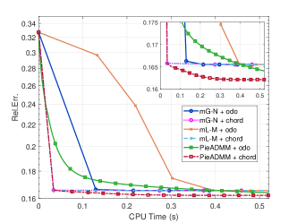
(a)

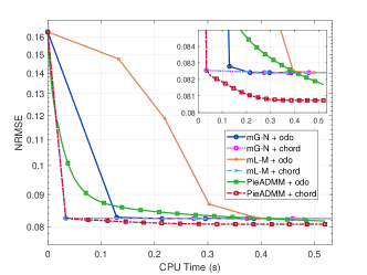
(b)

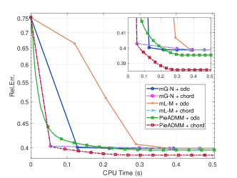
(c)

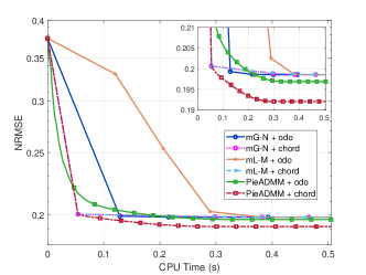
(d)

Figure 3: Performance of the three methods versus CPU time for circular ring datasets with $n=100$, $m=100$ under different initialization techniques . The noise level of the first row is $\sigma_{r}=0.01$ and $\sigma_{t}=0.05$, and the second row is $\sigma_{r}=0.03$ and $\sigma_{t}=0.1$.

Then, we compare these algorithms under additional noise levels and list the numerical results about Rel.Err, NRMSE and CPU time in Table II. We see that PieADMM costs less time and achieves better result.

TABLE II: Numerical results of different noise level of circular ring datasets with $m=n=100$, $m=100$.

		mG-N			mL-M			PieADMM
$\sigma_{r}$	$\sigma_{t}$	Rel.Err.	NRMSE	Time (s)	Rel.Err.	NRMSE	Time (s)	Rel.Err.	NRMSE	Time (s)
0.01	0.01	0.089	0.0443	0.31	0.089	0.0443	0.52	0.083	0.0413	0.16
	0.05	0.166	0.0824	0.32	0.166	0.0824	0.50	0.164	0.0814	0.18
	0.1	0.263	0.1310	0.32	0.263	0.1310	0.50	0.263	0.1309	0.15
	0.15	0.361	0.1795	0.32	0.361	0.1795	0.52	0.357	0.1778	0.37
	0.2	0.457	0.2277	0.40	0.457	0.2277	0.50	0.454	0.2263	0.35
0.03	0.01	0.236	0.1177	0.32	0.236	0.1177	0.50	0.233	0.1160	0.21
	0.05	0.306	0.1522	0.32	0.306	0.1523	0.50	0.304	0.1512	0.21
	0.1	0.399	0.1986	0.32	0.399	0.1986	0.51	0.398	0.1980	0.22
	0.15	0.492	0.2449	0.40	0.492	0.2449	0.51	0.489	0.2436	0.24
	0.2	0.584	0.2906	0.40	0.584	0.2906	0.59	0.583	0.2903	0.28
0.05	0.01	0.389	0.1938	0.32	0.389	0.1938	0.50	0.381	0.1895	0.28
	0.05	0.453	0.2255	0.32	0.453	0.2256	0.50	0.446	0.2220	0.28
	0.1	0.540	0.2690	0.40	0.540	0.2691	0.50	0.537	0.2672	0.28
	0.15	0.628	0.3127	0.40	0.628	0.3127	0.51	0.626	0.3115	0.28
	0.2	0.714	0.3555	0.40	0.714	0.3555	0.58	0.712	0.3547	0.28

We also test the impact of the number of poses $n$. In fact, since we limit the range of robot’s trajectory, the same level noise will cause a bigger impact when the number of vertices $n$ increase. Therefore, when comparing the influence of data size with different $n$, we use relative noise level as an unified standard, which means $\sigma_{r}=100\times\sigma_{r}^{rel}/n$ and $\sigma_{t}=100\times\sigma_{t}^{rel}/n$. The result is shown in Fig. 4. Fig. 4a and 4b show that the performance of PieADMM are flat, and sometimes slightly better, than the other two methods. However, the increasing of running time of PieADMM is much slower than them, see Fig. 4c. It is because that the scale of $n$ almost does not affect the cost of the rotation subproblems, which can be computed in parallel. Moreover, the translation subproblem concerns only matrix multiplication, and does not depend on the inverse of the matrix.

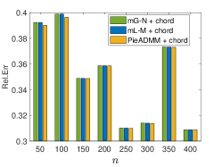
(a)

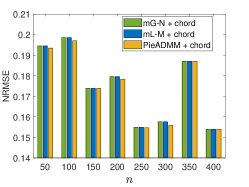
(b)

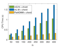
(c)

Figure 4: Performance of the three methods for circular ring datasets under different number of poses $n$. The relative noise level is $\sigma_{r}^{rel}=0.03$ and $\sigma_{t}^{rel}=0.1$.

For cube datasets, let $\sigma_{t}=\sigma_{t}^{rel}/\hat{n}$ where $\sigma_{t}^{rel}$ represent the relative noise level of translation. We first consider two examples with $\hat{n}=5$ or $8$, $\sigma_{r}=0.1,~{}\sigma_{t}^{rel}=0.1$ and $p_{cube}=0.3$. Fig. 5a and 5d shows the real trajectory, in which the blue lines are produced by motions and the red dotted lines are generated by observations. Fig. 5b, 5c and 5e, 5f are the noisy and recovered trajectory corresponding to different $\hat{n}$, respectively. The downward trends of Rel.Err along with CPU time are shown in Fig. 6, in which we omitted the top half of the image to highlight details. Since the PGO model is non-convex, and PieADMM is a non-monotonic algorithm, the curves may oscillate. However, it always converges to the solution with higher precision in less time.

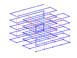
(a) Real trajectory

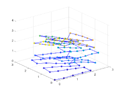
(b) Noisy trajectory

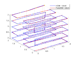
(c) Recovered trajectory

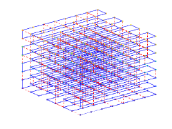
(d) Real trajectory

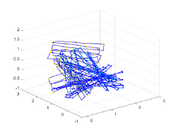
(e) Noisy trajectory

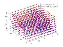
(f) Recovered trajectory

Figure 5: The comparison of cube trajectory, where the first row is $\hat{n}=5$ and the second row is $\hat{n}=8$, respectively. The color change of the vertices indicates the direction of the trajectory.

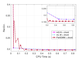
(a) $\hat{n}=5$

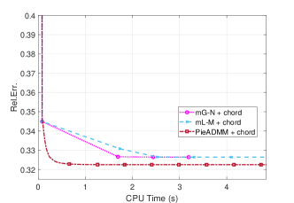
(b) $\hat{n}=8$

Figure 6: Performance of the three methods versus CPU time for cube datasets with $\hat{n}=5$ or $8$.

We also choose $\hat{n}$ from $2$ to $10$ and show the numerical results in Table III. Fig. 7a indicates the relationship between the number of edges and vertices of the cube datasets, and Fig. 7b and 7c illustrate the the upward trend of speed along with $\hat{n}$. The growth of cost of mG-N and mL-M are both cubic, and the growth of PieADMM is slower.

TABLE III: Numerical results of different $\hat{n}$ of cube datasets with $\sigma_{r}=0.1,~{}\sigma_{t}^{rel}=0.1$ and $p_{cube}=0.3$ or $0.7$.

		mG-N			mL-M			PieADMM
$\hat{n}$	$m$	Rel.Err.	NRMSE	Time (s)	Rel.Err.	NRMSE	Time (s)	Rel.Err.	NRMSE	Time (s)
$p_{cube}=0.3$
2	12	0.0803	0.1062	0.11	0.0803	0.1062	0.14	0.0791	0.1047	0.04
3	46	0.0854	0.1046	0.22	0.0854	0.1046	0.32	0.0848	0.1039	0.09
4	109	0.1596	0.1900	0.42	0.1596	0.1900	0.60	0.1576	0.1875	0.21
5	233	0.1969	0.2309	0.78	0.1969	0.2309	1.19	0.1955	0.2292	0.44
6	413	0.2343	0.2723	1.03	0.2343	0.2722	1.98	0.2342	0.2715	0.52
7	645	0.3083	0.3560	1.66	0.3083	0.3560	3.23	0.3074	0.3546	1.05
8	1024	0.3264	0.3752	2.37	0.3264	0.3752	4.82	0.3225	0.3708	1.66
9	1462	0.4312	0.4940	3.39	0.4312	0.4940	6.84	0.4309	0.4890	1.96
10	2025	0.6305	0.7205	4.52	0.6306	0.7205	9.48	0.6237	0.7127	2.22
$p_{cube}=0.7$
2	14	0.0540	0.0714	0.12	0.0540	0.0714	0.16	0.0539	0.0713	0.05
3	69	0.0614	0.0752	0.31	0.0614	0.0752	0.42	0.0614	0.0752	0.11
4	180	0.1338	0.1593	0.63	0.1338	0.1593	0.92	0.1262	0.1503	0.22
5	362	0.1244	0.1458	0.89	0.1244	0.1458	1.70	0.1177	0.1380	0.46
6	647	0.1542	0.1792	1.47	0.1542	0.1792	2.88	0.1521	0.1767	0.72
7	1096	0.2631	0.3038	2.43	0.2631	0.3038	4.87	0.2499	0.2885	1.41
8	1650	0.3212	0.3692	3.61	0.3212	0.3692	7.34	0.3068	0.3527	2.01
9	2418	0.2340	0.2681	5.12	0.2340	0.2681	10.68	0.2236	0.2562	2.58
10	3347	0.4295	0.4908	6.96	0.4295	0.4908	14.49	0.4268	0.4876	3.11

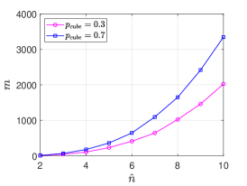
(a) number of edges

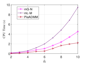
(b) $p_{cube}=0.3$

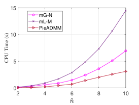
(c) $p_{cube}=0.7$

Figure 7: The trend of the numbers of edges and CPU time along with $\hat{n}$ with $\sigma_{r}=0.1,~{}\sigma_{t}^{rel}=0.1$ and $p_{cube}=0.3$ or $0.7$.

VI-B SLAM benchmark datasets

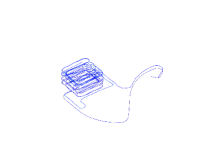
(a)

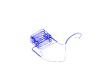
(b)

(c)

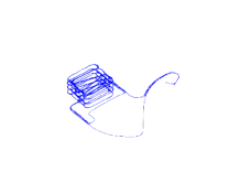
(d)

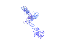
(e)

(f)

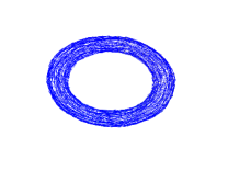
(g)

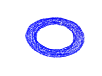
(h)

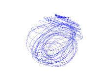
(i)

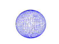
(j)

(k)

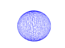
(l)

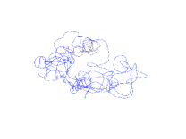
(m)

(n)

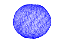
(o)

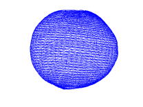
(p)

Noised data          mG-N           mL-M            PieADMM

Figure 8: The results of SLAM benchmark datasets in visual. The rows are the different data sets of garage, torus, sphere $1$ and sphere $2$, respectively. From the left column to the right column are the corrupted data and the recovered results by mG-N, mL-M, and PieADMM, respectively.

In this section, we test some popular 3D SLAM datasets. The garage dataset is a large-scale real-world example, and the other three (sphere $1$, sphere $2$ and torus) are common datasets used to compare performance. Different from sphere1 dataset, the larger noise is added to sphere2 dataset. We also use chordal initialization technique to compute an initial point for all methods. Fig. 8 shows the results of trajectory in visual, and the corresponding numerical results are listed in Table IV. It is worth noting that our model of rotation is based on the vMF distribution rather than the traditional Gaussian distribution, so the recovered solution is not the same, and it does not make sense to compare objective function values or gradients. We show the CPU time in the table, which indicates that PieADMM converges faster than mG-N and mL-M.

TABLE IV: The numerical results of SLAM benchmark datasets.

			CPU Time (s)
datasets	$n$	$m$	mG-N	mL-M	PieADMM
garage	1661	6275	17.31	32.24	14.37
sphere $1$	2500	4949	14.14	24.07	11.05
sphere $2$	2200	8647	24.08	38.02	17.95
torus	5000	9048	26.17	49.21	21.81

VII Conclusions

Pose graph optimization in SLAM is a special non-convex optimization, in which the variables are usually lies in $se(3)$ with nonlinear objective function, or a special Euclidean group with orthogonal constraints. The complex model makes it difficult to find a global solution.

In this paper, we propose a new non-convex pose graph optimization model based on augmented unit quaternion and von Mises-Fisher distribution, which is a large-scale quartic polynomial optimization on unit spheres. By introducing auxiliary variables, we reformulated it into a multi-quadratic polynomial optimization, multi-linear least square problem. Then we introduced a proximal linearized Riemannian ADMM for PGO model, in which the subproblems are simple projection problems, and can be solved in parallel corresponding to the structure of the directed graph, which greatly improve the efficiency. Then, based on the Lipschitz gradient continuity assumption which our PGO model satisfies and the first-order optimality conditions on manifolds, we establish the iteration complexity of $O(1/\epsilon^{2})$ for finding an $\epsilon$-stationary solution. The numerical experiments on two synthetic datasets with different data scales and noise level and four 3D SLAM benchmark datasets verify the effectiveness of our method.

Appendix A

We now add some definitions and lemmas which will be used in the following proofs. The concepts related to manifolds are shown in Appendix A.1 and we use spherical manifolds as a specific example. The optimization theories over manifolds are shown in Appendix A.2.

A.1 Manifolds

Suppose $\mathcal{M}$ is a differentiable manifold, then for any $x\in\mathcal{M}$, there exists a chart $(U,\varphi)$ in which $U$ is an open set with $x\in U\subseteq\mathcal{M}$ and $\phi$ is a homeomorphism between $U$ and an open set $\varphi(U)$ in Euclidean space. This coordinate transform enables us to locally treat a manifold as a Euclidean space. Next, we show the definition of tangent space which can help us get a linearized approximation around a point.

Definition A.1

(Tangent Space) Let $\mathcal{M}$ be a subset of a linear space, For all $x\in\mathcal{M}$, the tangent space is defined by

$$T_{x}\mathcal{M}=\left\{\gamma^{\prime}(0)\mid\gamma:I\rightarrow\mathcal{M}~{}\text{is smooth and}~{}\gamma(0)=x\right\},$$

where $I$ is any open interval containing zeros. That is, $v\in T_{x}\mathcal{M}$ if and only if there exists a smooth curve on $\mathcal{M}$ passing through $x$ with velocity $v$.

Define the set of all functions differentiable at point $x$ to be $\mathcal{F}_{x}$. An alternative but more general way of defining tangent space is by viewing a tangent vector $v\in T_{x}\mathcal{M}$ as an operator mapping $f\in\mathcal{F}_{x}$ to $v[f]\in\mathbb{R}$, which satisfies $v[f]=\frac{d(f(\gamma(t)))}{dt}\big{|}_{t=0}$. In other words, $v[f]$ computes the directional derivative of $f$ at $x$ along direction $v$. The tangent bundle of a manifold $\mathcal{M}$ is the disjoint union of the tangent spaces of $\mathcal{M}$, i.e.,

$$T\mathcal{M}=\{(x,v):x\in\mathcal{M}~{}\text{and}~{}v\in T_{x}\mathcal{M}\}.$$

Definition A.2

(Differential) The differential of $F:\mathcal{M}_{1}\rightarrow\mathcal{M}_{2}$ at the point $x\in\mathcal{M}_{1}$ is the linear map $DF(x):T_{x}\mathcal{M}_{1}\rightarrow T_{F(x)}\mathcal{M}_{2}$ defined by:

$$DF(x)[v]=\frac{d}{dt}F(\gamma(t))\bigg{|}_{t=0}=(F\circ\gamma)^{\prime}(0),$$

where $\gamma$ is a smooth curve on $\mathcal{M}_{2}$ passing through $x$ at $t=0$ with velocity $v$, and it satisfies

$$(DF(x)[v])[f]=v[f\circ F],~{}\text{for all}~{}v\in T_{x}\mathcal{M}_{1},~{}\text{and}~{}\forall f\in\mathcal{F}_{F(x)}.$$

Definition A.3

(Riemannian Manifold) A Riemannian manifold is a manifold which equip each tangent space of itself with a Riemannian metric $\left\langle\cdot,\cdot\right\rangle_{x}$ on $\mathcal{M}$ , and the metric varies smoothly with $x$.

When $\mathcal{M}$ is an embedded submanifolds of a linear space, $T_{x}\mathcal{M}$ coincides with the linear subspace. Furthermore, let $\left\langle\cdot,\cdot\right\rangle$ be the Euclidean metric on the linear space, the metric on $\mathcal{M}$ defined at each $x$ by restriction, $\left\langle u,v\right\rangle_{x}=\left\langle u,v\right\rangle$ for $u,v\in T_{x}\mathcal{M}$, is a Riemannian metric. At this point, we call $\mathcal{M}$ a Riemannian submanifold. Let $\mathcal{M}_{1}$, $\mathcal{M}_{2}$ be two Riemannian submanifolds, $\mathcal{M}_{1}\times\mathcal{M}_{2}$ is also a Riemannian submanifold with tangent spaces given by

$$T_{(x_{1},x_{2})}(\mathcal{M}_{1}\times\mathcal{M}_{2})=T_{x_{1}}\mathcal{M}_{1}\times T_{x_{2}}\mathcal{M}_{2}.$$

Definition A.4

(Riemannian Gradient) Let $f\in\mathcal{F}_{x}$. The Riemannian gradient of $f$ is the vector field $\operatorname{grad}f$ on $\mathcal{M}$ uniquely defined by the following identities:

$$\forall(x,v)\in T\mathcal{M},\quad Df(x)[v]=\left\langle v,\operatorname{grad}f(x)\right\rangle_{x}.$$

For an $m$-dimensional Riemannian submanifold $\mathcal{M}$, by defining $v=\gamma^{\prime}(0)$ and $v[f]=\left\langle\gamma^{\prime}(0),\nabla f(x)\right\rangle$, we have

$$\operatorname{grad}f(x)=\operatorname{Proj}_{T_{x}\mathcal{M}}(\nabla f(x)),$$

where $\operatorname{Proj}_{T_{x}\mathcal{M}}$ is the Euclidean projection operator onto the subspace $T_{x}\mathcal{M}$. Let $(U,\varphi)$ be a chart at $x\in\mathcal{M}$, then there exists a set of basis vectors $\{\bm{a}_{i}\}_{i=1}^{m}$ of $T_{x}\mathcal{M}$, such that for $v=\sum_{i=1}^{m}v_{i}\bm{a}_{i}$, we have

$$\hat{v}=D\varphi(x)[v]=(v_{1},\dots,v_{m}),\quad\hat{f}=f\circ\varphi,\quad\hat{x}=f(x),$$

where $\hat{o}$ denote the Euclidean counterpart of an object $o$ in $\mathcal{M}$. If we define the Gram matrix $G_{x}(i,j)=\left\langle\bm{a}_{i},\bm{a}_{j}\right\rangle_{x}$, then $\left\langle u,v\right\rangle_{x}=\hat{u}^{\top}G_{x}\hat{v}$.

When we regard the unit quaternion $\mathbb{U}$ as a sphere $\mathcal{S}^{3}$ embedded in $\mathbb{R}^{4}$, it is a Riemannian submanifold with the inherited metric $\left\langle u,v\right\rangle_{x}=\left\langle u,v\right\rangle=u^{\top}v$ and tangent space

$$T_{x}\mathbb{U}=\{v\in\mathbb{R}^{4}:x^{\top}v=0\}.$$

The Riemannian gradient of $f\in\mathcal{F}_{x}$ is

$$\operatorname{grad}f(x)=(I_{4}-xx^{\top})\nabla f(x).$$

A.2 Optimization theory over manifolds

Let $C$ be a nonempty closed subset in $\mathbb{R}^{n}$ and $x\in C$, the tangent cone is defined by $T_{C}(x):=\left\{y:\exists t_{k}\downarrow 0,x_{k}\rightarrow x,y_{k}\rightarrow y,~{}\text{s.t.}~{}x_{k}=x+t_{k}y_{k}\in C\right\}$. The normal cone is the dual cone of $-T_{C}(x)$ or the polar of $T_{C}(x)$, which is defined as $N_{C}(x):=\left\{z:z^{\top}y\leq 0,\forall y\in T_{C}(x)\right\}$. Suppose $S$ is a closed subset on the Riemannian manifold $\mathcal{M},(U,\varphi)$ is a chart at point $x\in S$, then by using coordinate transform , the Riemannian tangent cone can be defined as

$$T_{S}(x):=[D\varphi(x)]^{-1}\left[T_{\varphi(S\cap U)}(\varphi(x))\right].$$

Consequently, the Riemannian normal cone (see [61]) can be computed by

$$N_{S}(x)=[D\varphi(x)]^{-1}\left[G_{x}^{-1}N_{\varphi(U\cap S)}(\varphi(x))\right].$$

Lemma A.1

[50] Consider the following optimization problem over a manifold:

$$\min~{}f(x)\quad\text{s.t.}~{}x\in S\subset\mathcal{M},$$ (30)

$x^{*}$ is a stationary point if it satisfies

$$0\in\partial f(x^{*})+N_{S}(x^{*}).$$

where $\partial f$ is the Riemannian Clarke subdifferential defined in [61]. If f is differentiable, then the first-order optimality condition reduces to

$$-\operatorname{grad}f(x^{*})\in N_{S}(x^{*}),$$

or, equivalently

$$0=\operatorname{dist}(-\operatorname{grad}f(x^{*}),N_{S}(x^{*})).$$

If there exists equality constraints in problem (30), i.e. the feasible set can be described as $S=\Omega\cap X$, where $\Omega=\{x\in\mathcal{M}\mid c_{i}(x)=0,i=1,\dots m\}$ and $X$ is an nonempty bounded set. Then we have the following lemma:

Lemma A.2

[50] Suppose that $x^{*}\in\mathcal{M}$, $c_{i}(x^{*})=0,i=1,\dots m$, and

$$0\in\partial f(x^{*})+N_{\Omega}(x^{*})+N_{X}(x^{*}),$$ (31)

where

$$N_{\Omega}\left(x^{*}\right)=\left\{\sum_{i=1}^{m}\lambda_{i}\operatorname{grad}c_{i}\left(x^{*}\right)\mid\lambda\in\mathbb{R}^{m}\right\},$$

then $x^{*}$ is a stationary solution of problem (30).

Appendix B

We now show the proofs that are omitted from the paper.

Proof:

(a). Due to the non-negativity of $2$-norm, we have $f^{*}\geq 0,~{}g^{*}\geq 0$.

(b). We can rewrite the function $f$ as

$$f(\tilde{\bm{p}},\tilde{\bm{q}},\bm{t}) \!=\sum_{i=1}^{n}\sum_{(i,j)\in\mathcal{E}_{i}^{out}}\!\!\!\|M(\tilde{q}_{i})M(\tilde{t}_{ij})D\tilde{p}_{i}-(\tilde{t}_{j}-\tilde{t}_{i})\|_{\Sigma_{1}}^{2}.$$

Then, we have

$$\nabla_{\tilde{p}_{i}}f(\tilde{\bm{p}},\tilde{\bm{q}},\bm{t})$$

$$\!=\!\!\!\!\sum_{(i,j)\in\mathcal{E}_{i}^{out}}\!\!\!\!(M(\tilde{q}_{i})M(\tilde{t}_{ij})D)^{\!\top\!}\Sigma_{1}\left[M(\tilde{q}_{i})M(\tilde{t}_{ij})D\tilde{p}_{i}\!-\!(\tilde{t}_{j}\!-\!\tilde{t}_{i})\right],$$

and

$$\nabla_{\tilde{p}_{i}}^{2}f(\tilde{\bm{p}},\tilde{\bm{q}},\bm{t})\!=\!\!\!\sum_{(i,j)\in\mathcal{E}_{i}^{out}}\!\!\!(M(\tilde{q}_{i})M(\tilde{t}_{ij})D)^{\!\top\!}\Sigma_{1}M(\tilde{q}_{i})M(\tilde{t}_{ij})D.$$

It follows from Lemma II.2, and we have

$$\sigma_{\max}(\nabla_{\tilde{p}_{i}}^{2}f(\tilde{\bm{p}},\tilde{\bm{q}},\bm{t}))$$

$$\quad\leq\sigma_{\max}(\Sigma_{1})\sum_{(i,j)\in\mathcal{E}_{i}^{out}}\|\tilde{q}_{i}\|^{2}\|\tilde{t}_{ij}\|^{2}:=L_{f,\tilde{p}_{i}}(\tilde{\bm{q}}).$$ (32)

Let $L_{f,\tilde{\bm{p}}}(\tilde{\bm{q}}):=\max_{i}\{L_{f,\tilde{p}_{i}}(\tilde{\bm{q}})\}$, it is trivial that

$$\sigma_{\max}(\nabla_{\tilde{\bm{p}}}^{2}f(\tilde{\bm{p}},\tilde{\bm{q}},\bm{t}))\leq L_{f,\tilde{\bm{p}}}(\tilde{\bm{q}}),$$

which implies that our result holds. From (13), we obtain

$$f(\tilde{\bm{p}},\tilde{\bm{q}},\bm{t})=\|Q\bm{t}-\bm{s}\|_{I_{m}\otimes{\hat{\Sigma}_{1}}}^{2}+c(\tilde{\bm{p}},\tilde{\bm{q}}),$$

and $Q$ does not depend on $\tilde{\bm{p}}$, $\tilde{\bm{q}}$. The globally Lipschitz constants of $\nabla_{\bm{t}}f(\tilde{\bm{p}},\tilde{\bm{q}},\bm{t})$ is not hard to verify. The other globally Lipschitz constants are proven analogously.

(c). From (32), the result can be founded obviously.

(d). The result comes from that $\nabla f(\tilde{\bm{p}},\tilde{\bm{q}},\bm{t})$ is continuous and well defined on the closure of any bounded subset. The proof is completed. ∎

Proof:

Combining (19b) and (8d), we have

$$\bm{\lambda}^{k+1}\!=\!\!-\!\nabla_{\tilde{\bm{q}}}f(\tilde{\bm{p}}^{k+1},\tilde{\bm{q}}^{k+1},\bm{t}^{k})\!-\!\nabla_{\tilde{\bm{q}}}g(\tilde{\bm{p}}^{k+1},\tilde{\bm{q}}^{k+1})\!-\!H_{2}(\tilde{\bm{q}}^{k+1}-\tilde{\bm{q}}^{k}).$$ (33)

Hence,

$$\|\bm{\lambda}^{k+1}-\bm{\lambda}^{k}\|^{2}$$

$$\leq 4\|\nabla_{\tilde{\bm{q}}}f(\tilde{\bm{p}}^{k+1},\tilde{\bm{q}}^{k+1},\bm{t}^{k})-\nabla_{\tilde{\bm{q}}}f(\tilde{\bm{p}}^{k},\tilde{\bm{q}}^{k},\bm{t}^{k-1})\|^{2}$$

$$\quad+4\|\nabla_{\tilde{\bm{q}}}g(\tilde{\bm{p}}^{k+1},\tilde{\bm{q}}^{k+1})-\nabla_{\tilde{\bm{q}}}g(\tilde{\bm{p}}^{k},\tilde{\bm{q}}^{k})\|^{2}$$

$$\quad+4\|H_{2}(\tilde{\bm{q}}^{k+1}-\tilde{\bm{q}}^{k})\|^{2}+4\|H_{2}(\tilde{\bm{q}}^{k}-\tilde{\bm{q}}^{k-1})\|^{2}$$

$$\leq 4(L_{f}^{2}+L_{g}^{2})\|\tilde{\bm{p}}^{k+1}-\tilde{\bm{p}}^{k}\|^{2}+4L_{f}^{2}\|\bm{t}^{k}-\bm{t}^{k-1}\|^{2}$$

$$\quad+4\|\tilde{\bm{q}}^{k+1}-\tilde{\bm{q}}^{k}\|_{(L_{f}^{2}+L_{g}^{2})I+H_{2}^{\top}H_{2}}^{2}+4\|\tilde{\bm{q}}^{k}-\tilde{\bm{q}}^{k-1}\|_{H_{2}^{\top}H_{2}}^{2},$$

where the last inequality follows from (18). ∎

Proof:

It follows from (33), we have

$$\Phi^{k+1}$$

$$=f(\tilde{\bm{p}}^{k+1},\tilde{\bm{q}}^{k+1},\bm{t}^{k+1})+g(\tilde{\bm{p}}^{k+1},\tilde{\bm{q}}^{k+1})-\left\langle\bm{\lambda}^{k+1},\tilde{\bm{p}}^{k+1}-\tilde{\bm{q}}^{k+1}\right\rangle$$

$$\quad+\frac{\beta}{2}\|\tilde{\bm{p}}^{k+1}\!-\!\tilde{\bm{q}}^{k+1}\|^{2}\!+\!\|\tilde{\bm{q}}^{k+1}\!-\!\tilde{\bm{q}}^{k}\|_{\frac{4}{\beta}H_{2}^{\top}H_{2}}^{2}\!+\!\|\bm{t}^{k+1}-\bm{t}^{k}\|_{\frac{4}{\beta}L_{f}^{2}I}^{2}$$

$$=f(\tilde{\bm{p}}^{k+1},\tilde{\bm{q}}^{k+1},\bm{t}^{k+1})+g(\tilde{\bm{p}}^{k+1},\tilde{\bm{q}}^{k+1})+\frac{\beta}{2}\|\tilde{\bm{p}}^{k+1}-\tilde{\bm{q}}^{k+1}\|^{2}$$

$$\quad+\left\langle\nabla_{\tilde{\bm{q}}}f(\tilde{\bm{p}}^{k+1},\tilde{\bm{q}}^{k+1},\bm{t}^{k+1})+\nabla_{\tilde{\bm{q}}}g(\tilde{\bm{p}}^{k+1},\tilde{\bm{q}}^{k+1}),\tilde{\bm{p}}^{k+1}-\tilde{\bm{q}}^{k+1}\right\rangle$$

$$\quad+\left\langle\nabla_{\tilde{\bm{q}}}f(\tilde{\bm{p}}^{k+1},\tilde{\bm{q}}^{k+1},\bm{t}^{k})\!-\!\nabla_{\tilde{\bm{q}}}f(\tilde{\bm{p}}^{k+1},\tilde{\bm{q}}^{k+1},\bm{t}^{k+1}),\tilde{\bm{p}}^{k+1}\!-\!\tilde{\bm{q}}^{k+1}\right\rangle$$

$$\quad+\left\langle H_{2}(\tilde{\bm{q}}^{k+1}-\tilde{\bm{q}}^{k}),\tilde{\bm{p}}^{k+1}-\tilde{\bm{q}}^{k+1}\right\rangle$$

$$\quad+\|\tilde{\bm{q}}^{k+1}-\tilde{\bm{q}}^{k}\|_{\frac{4}{\beta}H_{2}^{\top}H_{2}}^{2}+\|\bm{t}^{k+1}-\bm{t}^{k}\|_{\frac{4}{\beta}L_{f}^{2}I}^{2}.$$

Since

$$\left\langle\nabla_{\tilde{\bm{q}}}f(\tilde{\bm{p}}^{k+1},\tilde{\bm{q}}^{k+1},\bm{t}^{k})\!-\!\nabla_{\tilde{\bm{q}}}f(\tilde{\bm{p}}^{k+1},\tilde{\bm{q}}^{k+1},\bm{t}^{k+1}),\tilde{\bm{p}}^{k+1}\!-\!\tilde{\bm{q}}^{k+1}\right\rangle$$

$$\geq-\frac{4}{\beta}\|\nabla_{\tilde{\bm{q}}}f(\tilde{\bm{p}}^{k+1},\tilde{\bm{q}}^{k+1},\bm{t}^{k})-\nabla_{\tilde{\bm{q}}}f(\tilde{\bm{p}}^{k+1},\tilde{\bm{q}}^{k+1},\bm{t}^{k+1})\|^{2}$$

$$\quad-\frac{\beta}{16}\|\tilde{\bm{p}}^{k+1}-\tilde{\bm{q}}^{k+1}\|^{2}$$

$$\geq-\frac{4L_{f}^{2}}{\beta}\|\bm{t}^{k+1}-\bm{t}^{k}\|^{2}-\frac{\beta}{16}\|\tilde{\bm{p}}^{k+1}-\tilde{\bm{q}}^{k+1}\|^{2},$$

and

$$\left\langle H_{2}(\tilde{\bm{q}}^{k+1}-\tilde{\bm{q}}^{k}),\tilde{\bm{p}}^{k+1}-\tilde{\bm{q}}^{k+1}\right\rangle$$

$$\geq-\frac{4}{\beta}\|\tilde{\bm{q}}^{k+1}-\tilde{\bm{q}}^{k}\|_{H_{2}^{\top}H_{2}}^{2}-\frac{\beta}{16}\|\tilde{\bm{p}}^{k+1}-\tilde{\bm{q}}^{k+1}\|^{2},$$

and the partial gradients $\nabla_{\tilde{\bm{q}}}f(\tilde{\bm{p}},\tilde{\bm{q}},\bm{t}),\nabla_{\tilde{\bm{q}}}g(\tilde{\bm{p}},\tilde{\bm{q}})$ are globally Lipschitz which satisfy (17), we can get

$$\Phi^{k+1} \geq f(\tilde{\bm{p}}^{k+1},\tilde{\bm{p}}^{k+1},\bm{t}^{k+1})+g(\tilde{\bm{p}}^{k+1},\tilde{\bm{p}}^{k+1})$$

$$\quad+\left(\frac{3\beta}{8}-\frac{L_{f,\tilde{\bm{q}}}}{2}-\frac{L_{g,\tilde{\bm{q}}}}{2}\right)\|\tilde{\bm{p}}^{k+1}-\tilde{\bm{q}}^{k+1}\|^{2}$$

$$\geq f^{*}+g^{*},$$

when $\beta>\frac{4}{3}(L_{f,\tilde{\bm{q}}}+L_{g,\tilde{\bm{q}}})$. The proof is completed. ∎

Proof:

From the subproblem (8a), we have

$$\mathcal{L}_{\beta}(\tilde{\bm{p}}^{k},\tilde{\bm{q}}^{k},\bm{t}^{k},\bm{\lambda}^{k})=\mathcal{L}_{\beta}^{k}(\tilde{\bm{p}}^{k},\tilde{\bm{q}}^{k},\bm{t}^{k},\bm{\lambda}^{k})$$

$$\geq\mathcal{L}_{\beta}^{k}(\tilde{\bm{p}}^{k+1},\tilde{\bm{q}}^{k},\bm{t}^{k},\bm{\lambda}^{k})+\frac{1}{2}\|\tilde{\bm{p}}^{k+1}-\tilde{\bm{p}}^{k}\|_{H_{1}}^{2}$$

$$\geq f(\tilde{\bm{p}}^{k+1},\tilde{\bm{q}}^{k},\bm{t}^{k})-\frac{L_{f,\tilde{\bm{p}}}}{2}\|\tilde{\bm{p}}^{k+1}-\tilde{\bm{p}}^{k}\|^{2}$$

$$\quad+g(\tilde{\bm{p}}^{k+1},\tilde{\bm{q}}^{k})-\frac{L_{g,\tilde{\bm{p}}}}{2}\|\tilde{\bm{p}}^{k+1}-\tilde{\bm{p}}^{k}\|^{2}$$

$$\quad-\left\langle\bm{\lambda}^{k},\tilde{\bm{p}}^{k+1}\!-\!\tilde{\bm{q}}^{k}\right\rangle\!+\!\frac{\beta}{2}\|\tilde{\bm{p}}^{k+1}\!-\!\tilde{\bm{q}}^{k}\|^{2}\!+\!\frac{1}{2}\|\tilde{\bm{p}}^{k+1}\!-\!\tilde{\bm{p}}^{k}\|_{H_{1}}^{2}$$

$$=\mathcal{L}_{\beta}(\tilde{\bm{p}}^{k+1},\tilde{\bm{q}}^{k},\bm{t}^{k},\bm{\lambda}^{k})+\frac{1}{2}\|\tilde{\bm{p}}^{k+1}-\tilde{\bm{p}}^{k}\|_{H_{1}-L_{f,\tilde{\bm{p}}}I-L_{g,\tilde{\bm{p}}}I}^{2},$$ (34)

where the second inequality follows from (7) and (17). From the subproblem (8b) and (8c), we obtain

$$\mathcal{L}_{\beta}(\tilde{\bm{p}}^{k+1},\tilde{\bm{q}}^{k},\bm{t}^{k},\bm{\lambda}^{k})-\mathcal{L}_{\beta}(\tilde{\bm{p}}^{k+1},\tilde{\bm{q}}^{k+1},\bm{t}^{k+1},\bm{\lambda}^{k})$$

$$\geq\frac{1}{2}\|\tilde{\bm{q}}^{k+1}-\tilde{\bm{q}}^{k}\|_{H_{2}}^{2}+\frac{1}{2}\|\bm{t}^{k+1}-\bm{t}^{k}\|_{H_{3}}^{2}.$$ (35)

Moreover, according to (8d),

$$\mathcal{L}_{\beta}(\tilde{\bm{p}}^{k+1},\tilde{\bm{q}}^{k+1},\bm{t}^{k+1},\bm{\lambda}^{k}) -\mathcal{L}_{\beta}(\tilde{\bm{p}}^{k+1},\tilde{\bm{q}}^{k+1},\bm{t}^{k+1},\bm{\lambda}^{k+1})$$

$$=-\frac{1}{\beta}\|\bm{\lambda}^{k+1}-\bm{\lambda}^{k}\|^{2}.$$ (36)

Combining (34)-(36) and Lemma V.1 yields that

$$~{}\mathcal{L}_{\beta}(\tilde{\bm{p}}^{k},\tilde{\bm{q}}^{k},\bm{t}^{k},\bm{\lambda}^{k})-\mathcal{L}_{\beta}(\tilde{\bm{p}}^{k+1},\tilde{\bm{q}}^{k+1},\bm{t}^{k+1},\bm{\lambda}^{k+1})$$

$$\geq\frac{1}{2}\|\tilde{\bm{p}}^{k+1}-\tilde{\bm{p}}^{k}\|_{H_{1}-L_{f,\tilde{\bm{p}}}I-L_{g,\tilde{\bm{p}}}I}^{2}+\frac{1}{2}\|\tilde{\bm{q}}^{k+1}-\tilde{\bm{q}}^{k}\|_{H_{2}}^{2}$$

$$\quad+\frac{1}{2}\|\bm{t}^{k+1}-\bm{t}^{k}\|_{H_{3}}^{2}-\frac{1}{\beta}\|\bm{\lambda}^{k+1}-\bm{\lambda}^{k}\|^{2}$$

$$\geq\|\tilde{\bm{p}}^{k+1}-\tilde{\bm{p}}^{k}\|_{\frac{1}{2}(H_{1}-L_{f,\tilde{\bm{p}}}I-L_{g,\tilde{\bm{p}}}I)-\frac{4}{\beta}(L_{f}^{2}+L_{g}^{2})I}^{2}$$

$$\quad+\|\bm{t}^{k+1}-\bm{t}^{k}\|_{\frac{1}{2}H_{3}}^{2}-\|\bm{t}^{k}-\bm{t}^{k-1}\|_{\frac{4}{\beta}L_{f}^{2}I}^{2}$$

$$\quad+\|\tilde{\bm{q}}^{k+1}-\tilde{\bm{q}}^{k}\|_{\frac{1}{2}H_{2}-\frac{4}{\beta}(L_{f}^{2}+L_{g}^{2})I-\frac{4}{\beta}H_{2}^{\top}H_{2}}^{2}$$

$$\quad-\|\tilde{\bm{q}}^{k}-\tilde{\bm{q}}^{k-1}\|_{\frac{4}{\beta}H_{2}^{\top}H_{2}}^{2},$$

which implies that

$$\Phi^{k} -\Phi^{k+1}$$

$$\geq\|\tilde{\bm{p}}^{k+1}-\tilde{\bm{p}}^{k}\|_{P_{1}}^{2}+\|\tilde{\bm{q}}^{k+1}-\tilde{\bm{q}}^{k}\|_{P_{2}}^{2}+\|\bm{t}^{k+1}-\bm{t}^{k}\|_{P_{3}}^{2}.$$

It is not hard to verify that when $\beta$ satisfies (27), $\{\Phi^{k}\}$ is monotonically nonincreasing. The proof is completed. ∎

Proof:

By summing (28) over $k=1,2,\dots,T$, we have

$$\Phi^{1}-\Phi^{T+1}\geq\sum_{k=1}^{T}\|\bm{w}^{k+1}-\bm{w}^{k}\|_{P}^{2}\geq\nu\sum_{k=1}^{T}\|\bm{w}^{k+1}-\bm{w}^{k}\|^{2},$$

which implies

$$\min_{2\leq k\leq T+1}\theta_{k}\leq\frac{1}{T}\sum_{k=2}^{T+1}\theta_{k}$$

$$=\frac{1}{T}\sum_{k=2}^{T+1}\|\bm{w}^{k+1}-\bm{w}^{k}\|^{2}+\frac{1}{T}\sum_{k=1}^{T}\|\bm{w}^{k+1}-\bm{w}^{k}\|^{2}$$

$$\leq\frac{1}{\nu T}(\Phi^{1}+\Phi^{2}-\Phi^{T+1}-\Phi^{T+2})\leq\frac{2}{\nu T}(\Phi^{1}-f^{*}-g^{*}).$$ (37)

By Lemma V.1,

$$\|\tilde{\bm{p}}^{k+1}-\tilde{\bm{q}}^{k+1}\|^{2}=\frac{1}{\beta^{2}}\|\bm{\lambda}^{k+1}-\bm{\lambda}^{k}\|^{2}$$

$$\leq\frac{4}{\beta^{2}}\left\{(L_{f}^{2}+L_{g}^{2})\|\tilde{\bm{p}}^{k+1}-\tilde{\bm{p}}^{k}\|^{2}+L_{f}^{2}\|\bm{t}^{k}-\bm{t}^{k-1}\|^{2}\right.$$

$$\quad\left.+\|\tilde{\bm{q}}^{k+1}-\tilde{\bm{q}}^{k}\|_{(L_{f}^{2}+L_{g}^{2})I+H_{2}^{\top}H_{2}}^{2}+\|\tilde{\bm{q}}^{k}-\tilde{\bm{q}}^{k-1}\|_{H_{2}^{\top}H_{2}}^{2}\right\}$$

$$\leq\kappa_{1}\theta_{k}.$$ (38)

According to (19c),

$$\|\nabla_{\bm{t}}f(\tilde{\bm{p}}^{k+1},\tilde{\bm{q}}^{k+1},\bm{t}^{k+1})\|^{2}=\|H_{3}(\bm{t}^{k+1}-\bm{t}^{k})\|^{2}\leq\kappa_{2}\theta_{k}.$$ (39)

From (19b), we have

$$\|\nabla_{\tilde{\bm{q}}}f(\tilde{\bm{p}}^{k+1},\tilde{\bm{q}}^{k+1},\bm{t}^{k+1})+\nabla_{\tilde{\bm{q}}}g(\tilde{\bm{p}}^{k+1},\tilde{\bm{q}}^{k+1})+\bm{\lambda}^{k+1}\|^{2}$$

$$\leq\|\nabla_{\tilde{\bm{q}}}f(\tilde{\bm{p}}^{k+1},\tilde{\bm{q}}^{k+1},\bm{t}^{k+1})-\nabla_{\tilde{\bm{q}}}f(\tilde{\bm{p}}^{k+1},\tilde{\bm{q}}^{k+1},\bm{t}^{k})$$

$$\quad-H_{2}(\tilde{\bm{q}}^{k+1}-\tilde{\bm{q}}^{k})\|^{2}$$

$$\leq 2L_{f}^{2}\|\bm{t}^{k+1}-\bm{t}^{k}\|^{2}+2\|\tilde{\bm{q}}^{k+1}-\tilde{\bm{q}}^{k}\|_{H_{2}^{\top}H_{2}}^{2}$$

$$\leq\kappa_{3}\theta_{k}.$$ (40)

From the first-order optimality conditions of $\tilde{\bm{p}}$-subproblem (19a), there exists some $\bm{s}^{k+1}\in N_{\mathbb{U}^{n}}(\tilde{\bm{p}}^{k+1})$ such that

$$\operatorname{Proj}_{T_{\tilde{\bm{p}}^{k+1}}\mathbb{U}^{n}}\left(\nabla_{\tilde{\bm{p}}}f(\tilde{\bm{p}}^{k},\tilde{\bm{q}}^{k},\bm{t}^{k})+\nabla_{\tilde{\bm{p}}}g(\tilde{\bm{p}}^{k},\tilde{\bm{q}}^{k})-\bm{\lambda}^{k}\right.$$

$$\quad\left.+\beta(\tilde{\bm{p}}^{k+1}-\tilde{\bm{q}}^{k})+H_{1}(\tilde{\bm{p}}^{k+1}-\tilde{\bm{p}}^{k})\right)+\bm{s}^{k+1}=0$$

which implies that $\bm{s}^{k+1}\in T_{\tilde{\bm{p}}^{k+1}}\mathbb{U}^{n}$. Therefore, we have

$$\operatorname{dist}\left(\operatorname{Proj}_{T_{\tilde{\bm{p}}^{k+1}}\mathbb{U}^{n}}\left\{-\nabla_{\tilde{\bm{p}}}f(\tilde{\bm{p}}^{k+1},\tilde{\bm{q}}^{k+1},\bm{t}^{k+1})\right.\right.$$

$$\quad\left.\left.-\nabla_{\tilde{\bm{p}}}g(\tilde{\bm{p}}^{k+1},\tilde{\bm{q}}^{k+1})+\bm{\lambda}^{k+1}\right\},N_{\mathbb{U}^{n}}(\tilde{\bm{p}}^{k+1})\right)$$

$$\leq\left\|\operatorname{Proj}_{T_{\tilde{\bm{p}}^{k+1}}\mathbb{U}^{n}}\left\{-\nabla_{\tilde{\bm{p}}}f(\tilde{\bm{p}}^{k+1},\tilde{\bm{q}}^{k+1},\bm{t}^{k+1})\right.\right.$$

$$\quad\left.\left.-\nabla_{\tilde{\bm{p}}}g(\tilde{\bm{p}}^{k+1},\tilde{\bm{q}}^{k+1})+\bm{\lambda}^{k+1}\right\}-\bm{s}^{k+1}\right\|$$

$$\leq\left\|-\nabla_{\tilde{\bm{p}}}f(\tilde{\bm{p}}^{k+1},\tilde{\bm{q}}^{k+1},\bm{t}^{k+1})-\nabla_{\tilde{\bm{p}}}g(\tilde{\bm{p}}^{k+1},\tilde{\bm{q}}^{k+1})\right.$$

$$\quad\left.+\nabla_{\tilde{\bm{p}}}f(\tilde{\bm{p}}^{k},\tilde{\bm{q}}^{k},\bm{t}^{k})+\nabla_{\tilde{\bm{p}}}g(\tilde{\bm{p}}^{k},\tilde{\bm{q}}^{k})\right.$$

$$\quad\left.+\beta(\tilde{\bm{q}}^{k+1}-\tilde{\bm{q}}^{k})+H_{1}(\tilde{\bm{p}}^{k+1}-\tilde{\bm{p}}^{k})\right\|$$

$$\leq\left\|\nabla_{\tilde{\bm{p}}}f(\tilde{\bm{p}}^{k+1},\tilde{\bm{q}}^{k+1},\bm{t}^{k+1})-\nabla_{\tilde{\bm{p}}}f(\tilde{\bm{p}}^{k},\tilde{\bm{q}}^{k},\bm{t}^{k})\right\|$$

$$\quad+\left\|\nabla_{\tilde{\bm{p}}}g(\tilde{\bm{p}}^{k+1},\tilde{\bm{q}}^{k+1})-\nabla_{\tilde{\bm{p}}}g(\tilde{\bm{p}}^{k},\tilde{\bm{q}}^{k})\right\|$$

$$\quad+\left\|\beta(\tilde{\bm{q}}^{k+1}-\tilde{\bm{q}}^{k})\right\|+\left\|H_{1}(\tilde{\bm{p}}^{k+1}-\tilde{\bm{p}}^{k})\right\|$$

$$\leq(L_{f}+L_{g}+\beta+\sigma_{\max}(H_{1}))\|\bm{w}^{k+1}-\bm{w}^{k}\|$$

$$\leq\sqrt{\kappa_{4}\theta_{k}},$$ (41)

where the second inequality follows the nonexpansive of projection operator and (8d). Combining (37)-(41), we can get the upper bound of iteration complexity of Algorithm 1. The proof is completed. ∎

Xin Chen received the B.S. degree from the Department of Mathematics of Jilin University, Changchun, China, in 2020. He is currently pursuing the Ph.D. degree with the School of Mathematical Sciences, Beihang University, Beijing, China. His research interests include the splitting algorithms for large-scale non-convex optimization problems and its applications in simultaneous localization and mapping and multi-dimensional data processing.

Chunfeng Cui is currently a tenure-track professor at the School of Mathematical Sciences, Beihang University. Her research interests include optimization theory and algorithms, tensor computations, dual quaternion and their applications. She has published more than 20 papers in journals and conferences such as SIAM series and IEEE series. She received her B.S. and Ph.D. degrees from Jilin University and Chinese Academy of Sciences, respectively. After graduating with a Ph.D., she worked as a postdoctoral researcher at City University of Hong Kong and University of California, Santa Barbara. In 2019, she won the Zhongjiaqing Mathematics Award of the Chinese Mathematical Society.

Deren Han is currently a professor, doctoral supervisor, and the dean of the School of Mathematical Sciences, Beihang University. He received the B.S. and Ph.D. degrees at Nanjing University, China, in 1997 and 2002, respectively. His research mainly focuses on numerical methods for large-scale optimization problems and variational inequality problems, as well as their applications in transportation planning and magnetic resonance imaging. He has published more than 150 papers in journals and conferences, and won the Youth Operations Research Award of Operations Research Society of China, the Second prize of Science and Technology Progress of Jiangsu Province and other awards. He has presided over the National Science Fund for Distinguished Young Scholars and other projects. Professor Deren Han also serves as the editorial board member of Numerical Computation and Computer Applications, Journal of the Operations Research Society of China, Journal of Global Optimization, Asia-Pacific Journal of Operational Research.

Liqun Qi is currently an Emeritus Professor of Applied Mathematics at the Hong Kong Polytechnic University and a professor at Hangzhou Dianzi University. He has published 390 papers in international journals. He established the superlinear convergence theory of semi-smooth Newton method and the global convergence theory of smooth newton method, and won the first prize of science and technology of Operations Research Society of China in 2010. Professor Liqun Qi’s papers are widely used in the world. He was listed as the most Cited Mathematicians in 2003-2010 and again in 2018, 2019, 2020 and 2021, respectively. Professor Liqun Qi serves as editor-in-chief or editorial board member of ten international magazines. Professor Liqun Qi published two monographs on tensor theory in 2017 and 2018 by SIAM and Springer Press, respectively.

References

- [1] C. Cadena, L. Carlone, H. Carrillo, Y. Latif, D. Scaramuzza, J. Neira, I. Reid, and J. J. Leonard, “Past, present, and future of simultaneous localization and mapping: Toward the robust-perception age,” IEEE Transactions on robotics, vol. 32, no. 6, pp. 1309–1332, 2016.
- [2] R. Smith, M. Self, and P. Cheeseman, “Estimating uncertain spatial relationships in robotics,” Autonomous robot vehicles, pp. 167–193, 1990.
- [3] A. J. Davison, I. D. Reid, N. D. Molton, and O. Stasse, “Monoslam: Real-time single camera SLAM,” IEEE transactions on pattern analysis and machine intelligence, vol. 29, no. 6, pp. 1052–1067, 2007.
- [4] W. Hess, D. Kohler, H. Rapp, and D. Andor, “Real-time loop closure in 2D lidar SLAM,” in 2016 IEEE international conference on robotics and automation (ICRA). IEEE, 2016, pp. 1271–1278.
- [5] S. Weiss and R. Siegwart, “Real-time metric state estimation for modular vision-inertial systems,” in 2011 IEEE international conference on robotics and automation. IEEE, 2011, pp. 4531–4537.
- [6] H. Durrant-Whyte and T. Bailey, “Simultaneous localization and mapping: part I,” IEEE Robotics Automation Magazine, vol. 13, no. 2, pp. 99–110, 2006.
- [7] A. Jurić, F. Kendeš, I. Marković, and I. Petrović, “A comparison of graph optimization approaches for pose estimation in slam,” in 2021 44th International Convention on Information, Communication and Electronic Technology (MIPRO). IEEE, 2021, pp. 1113–1118.
- [8] F. Lu and E. Milios, “Globally consistent range scan alignment for environment mapping,” Autonomous robots, vol. 4, pp. 333–349, 1997.
- [9] M. Montemerlo, S. Thrun, D. Koller, B. Wegbreit et al., “FastSLAM: A factored solution to the simultaneous localization and mapping problem,” Aaai/iaai, vol. 593598, 2002.
- [10] S. Thrun, Y. Liu, D. Koller, A. Y. Ng, Z. Ghahramani, and H. Durrant-Whyte, “Simultaneous localization and mapping with sparse extended information filters,” The international journal of robotics research, vol. 23, no. 7-8, pp. 693–716, 2004.
- [11] D. Wilbers, C. Merfels, and C. Stachniss, “A comparison of particle filter and graph-based optimization for localization with landmarks in automated vehicles,” in 2019 Third IEEE International Conference on Robotic Computing (IRC). IEEE, 2019, pp. 220–225.
- [12] L. Carlone, R. Tron, K. Daniilidis, and F. Dellaert, “Initialization techniques for 3D SLAM: A survey on rotation estimation and its use in pose graph optimization,” in 2015 IEEE international conference on robotics and automation (ICRA). IEEE, 2015, pp. 4597–4604.
- [13] E. Olson, J. Leonard, and S. Teller, “Fast iterative alignment of pose graphs with poor initial estimates,” in Proceedings 2006 IEEE International Conference on Robotics and Automation, 2006. ICRA 2006. IEEE, 2006, pp. 2262–2269.
- [14] G. Grisetti, C. Stachniss, and W. Burgard, “Nonlinear constraint network optimization for efficient map learning,” IEEE Transactions on Intelligent Transportation Systems, vol. 10, no. 3, pp. 428–439, 2009.
- [15] F. Dellaert and M. Kaess, “Square root SAM: Simultaneous localization and mapping via square root information smoothing,” The International Journal of Robotics Research, vol. 25, no. 12, pp. 1181–1203, 2006.
- [16] M. Kaess, A. Ranganathan, and F. Dellaert, “iSAM: Incremental smoothing and mapping,” IEEE Transactions on Robotics, vol. 24, no. 6, pp. 1365–1378, 2008.
- [17] M. Kaess, H. Johannsson, R. Roberts, V. Ila, J. J. Leonard, and F. Dellaert, “iSAM2: Incremental smoothing and mapping using the Bayes tree,” The International Journal of Robotics Research, vol. 31, no. 2, pp. 216–235, 2012.
- [18] G. Grisetti, R. Kümmerle, C. Stachniss, and W. Burgard, “A tutorial on graph-based SLAM,” IEEE Intelligent Transportation Systems Magazine, vol. 2, no. 4, pp. 31–43, 2010.
- [19] D. M. Rosen, M. Kaess, and J. J. Leonard, “An incremental trust-region method for robust online sparse least-squares estimation,” in 2012 IEEE International Conference on Robotics and Automation. IEEE, 2012, pp. 1262–1269.
- [20] R. Wagner, O. Birbach, and U. Frese, “Rapid development of manifold-based graph optimization systems for multi-sensor calibration and SLAM,” in 2011 IEEE/RSJ International Conference on Intelligent Robots and Systems. IEEE, 2011, pp. 3305–3312.
- [21] R. Kümmerle, G. Grisetti, H. Strasdat, K. Konolige, and W. Burgard, “G2o: A general framework for graph optimization,” in 2011 IEEE International Conference on Robotics and Automation, 2011, pp. 3607–3613.
- [22] J. Cheng, J. Kim, Z. Jiang, and W. Che, “Dual quaternion-based graphical SLAM,” Robotics and Autonomous Systems, vol. 77, pp. 15–24, 2016.
- [23] M. Liu, S. Huang, G. Dissanayake, and H. Wang, “A convex optimization based approach for pose SLAM problems,” in 2012 IEEE/RSJ International Conference on Intelligent Robots and Systems, 2012, pp. 1898–1903.
- [24] D. M. Rosen, C. DuHadway, and J. J. Leonard, “A convex relaxation for approximate global optimization in simultaneous localization and mapping,” in 2015 IEEE International Conference on Robotics and Automation (ICRA). IEEE, 2015, pp. 5822–5829.
- [25] L. Carlone, D. M. Rosen, G. Calafiore, J. J. Leonard, and F. Dellaert, “Lagrangian duality in 3D SLAM: Verification techniques and optimal solutions,” in 2015 IEEE/RSJ International Conference on Intelligent Robots and Systems (IROS). IEEE, 2015, pp. 125–132.
- [26] D. M. Rosen, L. Carlone, A. S. Bandeira, and J. J. Leonard, “SE-Sync: A certifiably correct algorithm for synchronization over the special euclidean group,” The International Journal of Robotics Research, vol. 38, no. 2-3, pp. 95–125, 2019.
- [27] T. Fan and T. Murphey, “Generalized proximal methods for pose graph optimization,” in The International Symposium of Robotics Research. Springer, 2019, pp. 393–409.
- [28] R. I. Hartley, J. Trumpf, Y. Dai, and H. Li, “Rotation averaging,” International Journal of Computer Vision, vol. 103, pp. 267–305, 2012.
- [29] L. Qi, X. Wang, and C. Cui, “Augmented quaternion and augmented unit quaternion optimization,” Accepted by Communications in Mathematical Sciences, 2024.
- [30] S. Sra, “A short note on parameter approximation for von Mises-Fisher distributions: and a fast implementation of ,” Computational Statistics, vol. 27, pp. 177–190, 2012.
- [31] S. Boyd, N. Parikh, E. Chu, B. Peleato, and J. Eckstein., “Distributed optimization and statistical learning via the alternating direction method of multipliers,” Foundations and Trends in Machine Learning, vol. 3, no. 1, pp. 1–122, 2011.
- [32] D. Han, “A survey on some recent developments of alternating direction method of multipliers,” Journal of the Operations Research Society of China, pp. 1–52, 2022.
- [33] J. B. Kuipers, Quaternions and rotation sequences: a primer with applications to orbits, aerospace, and virtual reality. Princeton university press, 1999.
- [34] Z. Chen, C. Ling, L. Qi, and H. Yan, “A regularization-patching dual quaternion optimization method for solving the hand-eye calibration problem,” Journal of Optimization Theory and Applications, pp. 1–23, 2024.
- [35] Y. Peng, A. Ganesh, J. Wright, W. Xu, and Y. Ma, “RASL: Robust alignment by sparse and low-rank decomposition for linearly correlated images,” IEEE transactions on pattern analysis and machine intelligence, vol. 34, no. 11, pp. 2233–2246, 2012.
- [36] M. Tao and X. Yuan, “Recovering low-rank and sparse components of matrices from incomplete and noisy observations,” SIAM Journal on Optimization, vol. 21, no. 1, pp. 57–81, 2011.
- [37] Z. Wen, C. Yang, X. Liu, and S. Marchesini, “Alternating direction methods for classical and ptychographic phase retrieval,” Inverse Problems, vol. 28, no. 11, p. 115010, 2012.
- [38] L. Yang, T. K. Pong, and X. Chen, “Alternating direction method of multipliers for nonconvex background/foreground extraction,” arXiv preprint arXiv:1506.07029, vol. 1, no. 5, p. 5, 2015.
- [39] R. Glowinski and A. Marroco, “Sur l’approximation, par éléments finis d’ordre un, et la résolution, par pénalisation-dualité d’une classe de problèmes de dirichlet non linéaires,” ESAIM: Mathematical Modelling and Numerical Analysis-Modélisation Mathématique et Analyse Numérique, vol. 9, no. R2, pp. 41–76, 1975.
- [40] D. Gabay and B. Mercier, “A dual algorithm for the solution of nonlinear variational problems via finite element approximation,” Computers Mathematics with Applications, vol. 2, no. 1, pp. 17–40, 1976.
- [41] D. Han and X. Yuan, “Local linear convergence of the alternating direction method of multipliers for quadratic programs,” SIAM Journal on numerical analysis, vol. 51, no. 6, pp. 3446–3457, 2013.
- [42] X. Cai, D. Han, and X. Yuan, “On the convergence of the direct extension of ADMM for three-block separable convex minimization models with one strongly convex function,” Computational Optimization and Applications, vol. 66, no. 1, pp. 39–73, 2017.
- [43] C. Chen, B. He, Y. Ye, and X. Yuan, “The direct extension of ADMM for multi-block convex minimization problems is not necessarily convergent,” Mathematical Programming, vol. 155, no. 1, pp. 57–79, 2016.
- [44] T. Lin, S. Ma, and S. Zhang, “On the global linear convergence of the ADMM with multiblock variables,” SIAM Journal on Optimization, vol. 25, no. 3, pp. 1478–1497, 2015.
- [45] K. Guo, D. Han, and T. Wu, “Convergence of alternating direction method for minimizing sum of two nonconvex functions with linear constraints,” International Journal of Computer Mathematics, vol. 94, no. 8, pp. 1653–1669, 2017.
- [46] A. Themelis and P. Patrinos, “Douglas–Rachford splitting and admm for nonconvex optimization: tight convergence results,” SIAM Journal on Optimization, vol. 30, no. 1, pp. 149–181, 2020.
- [47] M. Hong, Z.-Q. Luo, and M. Razaviyayn, “Convergence analysis of alternating direction method of multipliers for a family of nonconvex problems,” SIAM Journal on Optimization, vol. 26, no. 1, pp. 337–364, 2016.
- [48] C. Chen, M. Li, X. Liu, and Y. Ye, “Extended ADMM and BCD for nonseparable convex minimization models with quadratic coupling terms: convergence analysis and insights,” Mathematical Programming, vol. 173, pp. 37–77, 2019.
- [49] Y. Cui, X. Li, D. Sun, and K.-C. Toh, “On the convergence properties of a majorized alternating direction method of multipliers for linearly constrained convex optimization problems with coupled objective functions,” Journal of Optimization Theory and Applications, vol. 169, pp. 1013–1041, 2016.
- [50] J. Zhang, S. Ma, and S. Zhang, “Primal-dual optimization algorithms over Riemannian manifolds: an iteration complexity analysis,” Mathematical Programming, vol. 184, no. 1-2, pp. 445–490, 2020.
- [51] J. Li, S. Ma, and T. Srivastava, “A Riemannian ADMM,” arXiv preprint arXiv:2211.02163, 2022.
- [52] R. A. Fisher, “Dispersion on a sphere,” Proceedings of the Royal Society of London. Series A. Mathematical and Physical Sciences, vol. 217, no. 1130, pp. 295–305, 1953.
- [53] K. Hornik and B. Grün, “On maximum likelihood estimation of the concentration parameter of von Mises-Fisher distributions,” Computational statistics, vol. 29, pp. 945–957, 2014.
- [54] D. Gabay, “Minimizing a differentiable function over a differential manifold,” Journal of Optimization Theory and Applications, vol. 37, pp. 177–219, 1982.
- [55] S. T. Smith, “Optimization techniques on Riemannian manifolds,” Fields Institute Communications, vol. 3, 1994.
- [56] J. Hu, A. Milzarek, Z. Wen, and Y. Yuan, “Adaptive quadratically regularized Newton method for Riemannian optimization,” SIAM Journal on Matrix Analysis and Applications, vol. 39, no. 3, pp. 1181–1207, 2018.
- [57] J. Hu, X. Liu, Z. Wen, and Y. Yuan, “A brief introduction to manifold optimization,” Journal of the Operations Research Society of China, vol. 8, pp. 199–248, 2020.
- [58] Y. Ouyang, Y. Chen, G. Lan, and E. Pasiliao Jr, “An accelerated linearized alternating direction method of multipliers,” SIAM Journal on Imaging Sciences, vol. 8, no. 1, pp. 644–681, 2015.
- [59] X. Gao, B. Jiang, and S. Zhang, “On the information-adaptive variants of the admm: an iteration complexity perspective,” Journal of Scientific Computing, vol. 76, pp. 327–363, 2018.
- [60] B. He, L.-Z. Liao, D. Han, and H. Yang, “A new inexact alternating directions method for monotone variational inequalities,” Mathematical Programming, vol. 92, pp. 103–118, 2002.
- [61] W. Yang, L. Zhang, and R. Song, “Optimality conditions for the nonlinear programming problems on Riemannian manifolds,” Pacific Journal of Optimization, vol. 10, no. 2, pp. 415–434, 2014.