Doubly Adaptive Importance Sampling

Abstract

We propose an adaptive importance sampling scheme for Gaussian approximations of intractable posteriors. Optimization-based approximations like variational inference can be too inaccurate while existing Monte Carlo methods can be too slow. Therefore, we propose a hybrid where, at each iteration, the Monte Carlo effective sample size can be guaranteed at a fixed computational cost by interpolating between natural-gradient variational inference and importance sampling. The amount of damping in the updates adapts to the posterior and guarantees the effective sample size. Gaussianity enables the use of Stein’s lemma to obtain gradient-based optimization in the highly damped variational inference regime and a reduction of Monte Carlo error for undamped adaptive importance sampling. The result is a generic, embarrassingly parallel and adaptive posterior approximation method. Numerical studies on simulated and real data show its competitiveness with other, less general methods.

Keywords: Adaptive Monte Carlo; Embarrassingly parallel computing; Gaussian posterior approximation; Natural-gradient variational inference; Stein’s lemma

1 Introduction

It is common in several modelling settings to encounter distributions that are only known up to proportionality. Some examples are models characterized by an intractable likelihood, complex prior specifications or general non-conjugate Bayesian models. The goal of this work is to propose a novel approach to approximate a $\mathbb{R}^{d}$-valued probability distribution $\pi$ for which the normalizing constant is unknown in closed form. Although the distribution $\pi$ can be approximated by numerical integration in low-dimensional settings, the problem is typically challenging in higher dimensions due to the curse of dimensionality. Popular approximation schemes include optimization-based methods such as Laplace approximation, variational inference (VI, Blei et al., 2017) and expectation propagation (EP, Minka, 2001), as well as Monte Carlo (MC) approaches such as Markov chain MC, (adaptive) importance sampling (IS, Bugallo et al., 2017) or sequential Monte Carlo (SMC, Del Moral et al., 2006). However, optimization-based approximations are often too inaccurate while MC can be computationally too expensive. This motivates hybrid approaches that blend features of optimization and MC methods (Jerfel et al., 2021). We propose a novel hybrid method that adaptively interpolates between the computational speed and approximate nature of VI (Khan and Nielsen, 2018) and the accuracy and computational cost of IS.

The task of approximating a density known only up to proportionality typically arises in Bayesian statistics, where intractable posterior distributions are commonly encountered. Let $x\in\mathbb{R}^{d}$ indicate a $d$-dimensional parameter vector and $y\in\mathbb{R}^{n}$ be the data, so that $\ell(y\!\mid\!x)$ provides the model likelihood. Let $p_{0}$ be the prior distribution of the parameter $x$ and $p_{y}$ the marginal density of $y$. Then, by Bayes’ rule, the posterior distribution of $x$ given $y$ is obtained as $\pi(x)=\ell(y\!\mid\!x)\,p_{0}(x)/p_{y}(y)$, where we indicate the distributions and the corresponding densities with the same symbols. The normalizing constant $p_{y}(y)$ of the posterior density $\pi$ is often intractable and cumbersome to approximate in high-dimensional settings, such as Bayesian inverse problems (Stuart, 2010).

We devise an adaptive IS (AIS) scheme that iteratively adapts a proposal distribution by matching sufficient statistics while concurrently adapting an annealed version of the target distribution. The annealed version of the target distribution is obtained through a damping mechanism that guarantees a target effective sample size (ESS) used for quantifying the MC error. In particular, the damping parameter, which specifies the annealing at each iteration of the algorithm, is obtained by numerically solving a fixed lower bound on the ESS. The two types of adaptation motivate the name doubly adaptive importance sampling (DAIS). The proposed approach is based on IS and can consequently easily leverage parallel computations and modern compute environments. For concreteness, we mainly focus on Gaussian proposals although the methodology can be adapted to more general scenarios. In the Gaussian setting, we use Stein’s lemma to build a variance reduction scheme that significantly enhances the robustness of the proposed method.

We set the proposed methodology in the context of variational inference (VI). In its most common form, VI determines an approximating distribution $q$ by minimizing the Kullback-Leibler (KL) divergence $\mathrm{KL}{\left(\,q\,\|\,\pi\,\right)}$ of $\pi$ from $q$ over a tractable family of distributions. The quantity $\mathrm{KL}{\left(\,q\,\|\,\pi\,\right)}$, often referred to as the reverse KL divergence, involves an expectation with respect to the tractable approximating distribution $q$. While it is relatively straightforward to implement VI, the use of the reverse KL divergence is known to often yield an approximating distribution $q$ with lower variance than $\pi$ (Minka, 2005; Li and Turner, 2016; Jerfel et al., 2021) and thus overconfident Bayesian inference. Minimizing the forward KL divergence $\mathrm{KL}{\left(\,\pi\,\|\,q\,\right)}$ can mitigate these issues but is typically computationally challenging since it involves an expectation with respect to the intractable distribution $\pi$. Linking both extremes, the $\alpha$-divergence $\mathrm{K}_{\alpha}{\left(\,\pi\,\|\,q\,\right)}$ (Amari, 1985; Minka, 2005; Li and Turner, 2016) interpolates between the reverse and the forward KL divergences using the parameter $\alpha$. We show that the fixed points of DAIS’ iterative procedure can be described as a stationary point of the functional $q\mapsto\mathrm{K}_{\alpha}{\left(\,\pi\,\|\,q\,\right)}$ for a parameter $0<\alpha<1$ related to the amount of damping used within our method. The proposed adaptive damping scheme thus produces an automatic trade-off between minimizing the computationally more convenient reverse KL divergence and the forward KL divergence, which yields more accurate approximations. Finally, we establish that in the limit of maximally damped updates (i.e. slow updates), our method corresponds to minimizing the reverse KL divergence $\mathrm{KL}{\left(\,q\,\|\,\pi\,\right)}$ with a natural-gradient descent scheme.

The rest of this article is organized as follows. Section 2 introduces DAIS. Section 3 discusses related work. Section 4 analyses the link with natural-gradient VI and $\alpha$-divergence. Section 5 presents empirical results. Section 6 concludes.

2 Doubly Adaptive Importance Sampling

2.1 Algorithm Setting and Notation

We consider a target distribution $\pi(dx)=\pi(x)dx$ on $\mathbb{R}^{d}$ with strictly positive and continuously differentiable density $\pi(x)$ with respect to the Lebesgue measure $dx$. We constrain ourselves to building Gaussian approximations of $\pi$, although parts of our development also apply to other families of approximating distributions, as discussed in Section 6. DAIS iteratively builds a sequence of Gaussian approximations to the target distribution $\pi$. At iteration $t\geq 1$, the current Gaussian approximation is denoted by $q_{t}\equiv\mathcal{N}\left(\mu_{t},\Gamma_{t}\right)$ for a mean vector $\mu_{t}\in\mathbb{R}^{d}$ and positive-definite covariance matrix $\Gamma_{t}\in\mathbb{S}^{d}$. DAIS requires the log-target density $\log\pi(x)$ to be known up to an additive constant and its gradient $\nabla\!_{x}\log\pi(x)$ to be efficiently evaluated.

Throughout the article, we denote expectations with respect to a distribution $\eta(dx)$ by $\mathbb{E}_{\eta}[\varphi(X)]=\int\varphi(x)\,\eta(dx)$. For two vectors $u,v\in\mathbb{R}^{d}$, we indicate their inner product by $\left<u,v\right>=\sum\limits_{i=1}^{d}u_{i}v_{i}$, and their outer product by $u\otimes v\equiv u\,v^{\top}\in\mathbb{R}^{d\times d}$. For two vector-valued functions $U:\mathbb{R}^{d}\to\mathbb{R}^{d_{U}}$ and $V:\mathbb{R}^{d}\to\mathbb{R}^{d_{V}}$, and an $\mathbb{R}^{d}$-valued random variable $X$ with distribution $\eta(dx)$, the covariance matrix between the random variables $U(X)$ and $V(X)$ is denoted as $\mathrm{cov}_{\eta}[U(X),V(X)]\in\mathbb{R}^{d_{U}\times d_{V}}$. The subspace of $d$-dimensional symmetric matrices is denoted by $\mathbb{S}^{d}$. Finally, the KL divergence between two probability distributions $p\ll q$ is defined as $\mathrm{KL}{\left(\,p\,\|\,q\,\right)}=\mathbb{E}_{p}[\log\{(dp/dq)(X)\}]$.

2.2 Adaptive Gaussian Approximations

We can assess the quality of the approximation to the target distribution $\pi(x)$ by measuring the closeness of the two probability distributions. This can be done in different ways, such as minimizing the forward or reverse KL divergences. These divergences measure closeness differently. DAIS builds a Gaussian approximation $q_{\star}$ to the target distribution whose first two moments are matched to those of $\pi$. This corresponds to minimizing the forward KL,

$$q_{\star}\;=\;\mathrm{argmin}\;{\left\{\mathrm{KL}{\left(\,\pi\,\|\,q\,\right)}\;:\;q\in\mathcal{Q}_{\mathrm{gauss}}\right\}},$$ (1)

where $\mathcal{Q}_{\mathrm{gauss}}$ denotes the exponential family of Gaussian distributions. This objective is desirable in a Bayesian setting as the posterior mean and covariance are often of interest.

The DAIS procedure is initialized from a user-specified Gaussian approximation $q_{1}=\mathcal{N}\left(\mu_{1},\Gamma_{1}\right)$. Approaches for setting the initial approximation include using (a Gaussian approximation to) the prior distribution, or a Laplace approximation to the target distribution $\pi$, although more sophisticated procedures are possible.

Given the current approximation $q_{t}$, an improved Gaussian approximation $q_{t+1}$ is obtained by evaluating the first two moments of an annealed distribution $q_{t,\varepsilon_{t}}$ that interpolates between the current Gaussian distribution $q_{t}$ and the target distribution $\pi$. The intermediate distribution, defined as $q_{t,\varepsilon_{t}}(x)\propto q_{t}^{1-\varepsilon_{t}}(x)\,\pi^{\varepsilon_{t}}(x)$, is coined the damped target density in analogy with damped expectation propagation (EP) (Vehtari et al., 2020, Section 5.2). The parameter $0<\varepsilon_{t}<1$ is referred to as the damping parameter and we have that

$$q_{t,\varepsilon_{t}}(x)\propto q_{t}(x)\,e^{\varepsilon_{t}\Phi_{t}(x)}\qquad\textrm{for}\qquad\Phi_{t}(x)=\log\pi(x)-\log q_{t}(x).$$ (2)

The function $\Phi_{t}:\mathbb{R}^{d}\to\mathbb{R}$ captures the discrepancy between the current approximation $q_{t}$ and the target distribution $\pi$. Since DAIS only requires the gradient of $\Phi_{t}$, the target distribution can be specified up to a multiplicative constant. The first two moments $\mu_{t,\varepsilon_{t}}=\mathbb{E}_{q_{t,\varepsilon_{t}}}[X]$ and $\Gamma_{t,\varepsilon_{t}}=\mathrm{cov}_{q_{t,\varepsilon_{t}}}[X]\in\mathbb{S}^{d}$ of the damped target density $q_{t,\varepsilon_{t}}$ can be expressed as perturbations of the current parameters $\mu_{t}$ and $\Gamma_{t}$:

$$\left\{\begin{aligned} \mu_{t,\varepsilon_{t}}&=\mu_{t}+\varepsilon_{t}\,\mathbf{G}_{\mu}(q_{t},\varepsilon_{t})\\ \Gamma_{t,\varepsilon_{t}}&=\Gamma_{t}+\varepsilon_{t}\,\mathbf{G}_{\Gamma}(q_{t},\varepsilon_{t})\end{aligned}\right.\quad\text{where}\quad\left\{\begin{aligned} \mathbf{G}_{\mu}(q_{t},\varepsilon_{t})&=\mathbb{E}_{q_{t,\varepsilon_{t}}}[\Gamma_{t}\nabla\Phi_{t}(X)]\in\mathbb{R}^{d}\\ \mathbf{G}_{\Gamma}(q_{t},\varepsilon_{t})&=\mathrm{cov}_{q_{t,\varepsilon_{t}}}[\Gamma_{t}\nabla\Phi_{t}(X),X]\in\mathbb{S}^{d}.\end{aligned}\right.$$ (3)

The proof of the identities in (3) is presented in Section 2.3 and Appendix LABEL:ap:Stein. Furthermore, Section 4 connects the quantities $\mathbf{G}_{\mu}(q_{t},\varepsilon_{t})$ and $\mathbf{G}_{\Gamma}(q_{t},\varepsilon_{t})$ to the (negative) natural gradients of both the functionals $q_{t}\mapsto\mathrm{KL}{\left(\,q_{t}\,\|\,\pi\,\right)}$ and $q_{t}\mapsto\mathrm{KL}{\left(\,\pi\,\|\,q_{t}\,\right)}$.

Since both $\mathbf{G}_{\mu}(q_{t},\varepsilon_{t})$ and $\mathbf{G}_{\Gamma}(q_{t},\varepsilon_{t})$ are expressed as expectations with respect to the damped target density $q_{t,\varepsilon_{t}}$, these quantities can be estimated as $\widehat{\mathbf{G}}_{\mu}(q_{t},\varepsilon_{t})$ and $\widehat{\mathbf{G}}_{\Gamma}(q_{t},\varepsilon_{t})$ with self-normalized IS with $S\geq 1$ samples generated from a proposal distribution $\overline{q}_{t}(dx)$. In all our experiments we opt for the simple choice $\overline{q}_{t}(dx)=q_{t}(dx)$, although more robust alternatives (e.g. multivariate $t$-distribution with location $\mu_{t}$ and scale $\Gamma_{t}$) are possible, and methods for regularizing the IS weights could be applied (Vehtari et al., 2024).

The damping parameter $0<\varepsilon_{t}\leq 1$ that controls the closeness of the intermediate distribution $q_{t,\varepsilon_{t}}$ to the target distribution $\pi$ is chosen adaptively so that the ESS is above a user-specified threshold $1<N_{\mathrm{ESS}}<S$. Given $S$ samples $x_{t,1:S}=(x_{t,1},\ldots,x_{t,S})$ from the proposal distribution $q_{t}$, the associated ESS is computed as:

$$\mathrm{ESS}(W^{\varepsilon}_{t,1:S})=\frac{\big{(}\sum_{s}W^{\varepsilon}_{t,s}\big{)}^{2}}{\sum_{s}(W^{\varepsilon}_{t,s})^{2}}\qquad\text{with}\qquad W^{\varepsilon}_{t,s}=\frac{q_{t,\varepsilon}(x_{t,s})}{q_{t}(x_{t,s})}.$$ (4)

Since $\varepsilon\mapsto\mathrm{ESS}(W^{\varepsilon}_{t,1:S})$ is a continuous and decreasing function of $0<\varepsilon\leq 1$ (Beskos et al., 2016, Lemma 3.1), the optimal damping parameter at iteration $t$ can efficiently be computed with a standard root-finding method such as the bisection method, solving:

$$\varepsilon_{t}=\max\Big{\{}\varepsilon\in(0,1]\;:\;\mathrm{ESS}(W^{\varepsilon}_{t,1:S})\geq N_{\mathrm{ESS}}\Big{\}}.$$ (5)

As explained in Section 4, the quantities $\mathbf{G}_{\mu}(q_{t},\varepsilon_{t})$ and $\mathbf{G}_{\Gamma}(q_{t},\varepsilon_{t})$ can heuristically be thought of as (natural) gradients. This motivates the updates

$$\left\{\begin{aligned} \mu_{t+1}&=\mu_{t}+\zeta_{t}\,\widehat{\mathbf{G}}_{\mu}(q_{t},\varepsilon_{t})\\ \Gamma_{t+1}&=\Gamma_{t}+\zeta_{t}\,\widehat{\mathbf{G}}_{\Gamma}(q_{t},\varepsilon_{t})\end{aligned}\right.$$ (6)

for a sequence of learning rates $\zeta_{t}>0$. The choice $\zeta_{t}=\varepsilon_{t}$ corresponds to matching the first two moments of $q_{t+1}$ to the (estimate of) the first two moments of the damped target distribution $q_{t,\varepsilon_{t}}$. Since $\widehat{\mathbf{G}}_{\mu}(q_{t},\varepsilon_{t})\in\mathbb{R}^{d}$ and $\widehat{\mathbf{G}}_{\Gamma}(q_{t},\varepsilon_{t})\in\mathbb{S}^{d}$ are only stochastic estimates, for improved robustness, we advocate choosing $\zeta_{t}=\gamma\,\varepsilon_{t}$ for a parameter $0<\gamma\leq 1$.

In the event that the updated covariance $\Gamma_{t}+\zeta_{t}\,\widehat{\mathbf{G}}_{\Gamma}(q_{t},\varepsilon_{t})$ is not positive-definite, standard post-processing methods can be used for transforming the estimate into a positive-definite version of it. Possible approaches include setting the negative eigenvalues to small positive numbers. A more principled approach consists in reducing the damping parameter $\varepsilon_{t}$. Since the computational bottleneck generally lies in the evaluation of the target density $\pi$, recomputing the mean and covariance estimates for a reduced damping parameter $\varepsilon_{t}$ is generally computationally straightforward since no additional evaluation of the target density $\pi$ is necessary.

2.3 Control Variate for Gaussian Perturbations

Since $q_{t,\varepsilon_{t}}$ is a perturbation of the current Gaussian approximation $q_{t}$, estimating the moments $\mu_{t,\varepsilon_{t}}$ and $\Gamma_{t,\varepsilon_{t}}$ from scratch is statistically suboptimal. Instead, we derive update equations using Stein’s (1972) identity: for a probability density $p(x)$ on $\mathbb{R}^{d}$ and a continuously differentiable test function $\varphi:\mathbb{R}^{d}\to\mathbb{R}^{d}$, we have that (Oates et al., 2017, Proposition 2)

$$\mathbb{E}_{p}{\left[{\left(\left<\nabla\log p,\varphi\right>+\mathrm{div}\varphi\right)}(X)\right]}=0$$ (7)

Equation (7) follows from an integration by parts that is justified under mild growth and regularity assumptions (Mira et al., 2013; Oates et al., 2017). As derived in Appendix LABEL:ap:Stein, applying (7) to the annealed density $q_{t,\varepsilon_{t}}$ and appropriate test functions gives:

$$\mathbb{E}_{q_{t,\varepsilon_{t}}}[X] =\mu_{t}+\varepsilon_{t}\,\Gamma_{t}\,\mathbb{E}_{q_{t,\varepsilon_{t}}}{\left[\nabla\Phi_{t}(X)\right]}$$ (8a)

$$\mathrm{cov}_{q_{t,\varepsilon_{t}}}[X] =\Gamma_{t}+\varepsilon_{t}\,\Gamma_{t}\,\mathrm{cov}_{q_{t,\varepsilon_{t}}}[\nabla\Phi_{t}(X),X].$$ (8b)

These identities show that, given knowledge of $\mu_{t}$ and $\Gamma_{t}$, the first two moments of $q_{t,\varepsilon_{t}}$ can be estimated with a root-mean-square error (RMSE) of order $\varepsilon_{t}/\sqrt{S}$ as $\varepsilon_{t}\to 0$ when using $S$ samples (Owen, 2013) to estimate the right-hand sides of (8). A standard IS procedure that estimates these two quantities from scratch (i.e. without exploiting knowledge of $\mu_{t}$ and $\Gamma_{t}$) would typically lead to a RMSE of order $1/\sqrt{S}$ as $\varepsilon_{t}\to 0$, i.e. the MC error does not vanish as $\varepsilon_{t}\to 0$. Furthermore, when $q_{t}$ is a good approximation to the target distribution $\pi$, which is expected as the DAIS procedure progresses, the discrepancy function $\Phi_{t}$ and its gradient typically become small, leading to improved robustness.

We conclude this section by illustrating the statistical advantages of estimating the first two moments $\mu_{t,\varepsilon_{t}}$ and $\Gamma_{t,\varepsilon_{t}}$ of $q_{t,\varepsilon_{t}}$ through (8) when compared to a naive IS estimation of these two quantities. For this purpose, we consider a tractable setting where $q_{t}=\mathcal{N}(0,\mathrm{I}_{d})$ is a standard isotropic distribution of dimension $d=10$ and the target distribution is also Gaussian $\pi=\mathcal{N}\left(m,\Sigma\right)$ with mean $m=(1,\ldots,1)$ and covariance $\Sigma$ with $\Sigma_{i,j}=0.9+0.1\,{\delta(i=j)}$. Figure 1 reports, as a function of $\varepsilon_{t}$, the RMSE quantities $\mathbb{E}[\|\widehat{\mu}_{t,\varepsilon_{t}}-\mu_{t,\varepsilon_{t}}\|^{2}]^{1/2}$ and $\mathbb{E}[\|\widehat{\Gamma}_{t,\varepsilon_{t}}-\Gamma_{t,\varepsilon_{t}}\|_{\mathrm{F}}^{2}]^{1/2}$, where $\|M\|_{\mathrm{F}}^{2}=\sum M_{i,j}^{2}$ is the squared Frobenius norm of the matrix $M$. The RMSEs are approximated with $10^{2}$ independent experiments and the IS estimates use $S=10^{2}$ particles.

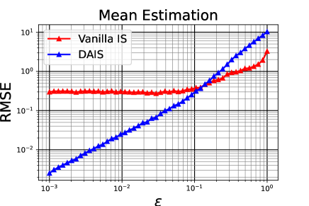
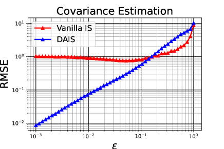
Figure 1: Estimation of $\widehat{\mu}_{t,\varepsilon_{t}}$ and $\widehat{\Gamma}_{t,\varepsilon_{t}}$ as a function of $\varepsilon_{t}$ with standard self-normalized IS and with DAIS based on (3) with $S=10^{2}$ particles. The proposal $q_{t}=\mathcal{N}(0,\mathbf{1}_{D})$ is a standard isotropic distribution in dimension $D=10$ and the target distribution is also Gaussian $\pi=\mathcal{N}(m,\Sigma)$ with mean $m=(1,\ldots,1)\in\mathbb{R}^{D}$ and covariance $\Sigma\in\mathbb{S}^{D}$ with $\Sigma_{i,j}=0.9+0.1\,\delta(i=j)$.

2.4 Monitoring Convergence

In challenging settings where the target distribution departs significantly from Gaussianity, running DAIS with a fixed number of IS particles $S$ per iteration produces a sequence of damping parameters $\varepsilon_{t}$ that does not eventually converge to one. Furthermore, it is typically not feasible to reliably estimate the forward KL divergence $\mathrm{KL}{\left(\,\pi\,\|\,q_{t}\,\right)}$ with MC methods. Instead, experiments suggest monitoring the damping parameter $\varepsilon_{t}$ defined in (5). Although the trajectory $t\mapsto\varepsilon_{t}$ is typically noisy and not necessarily increasing, we observe that the damping parameter eventually (and often rapidly) reaches a stationary regime, indicating convergence. For monitoring convergence, another option is tracking the Evidence Lower BOund

$$\mathrm{ELBO}(q_{t})=\int_{x}\log{\left\{\frac{\overline{\pi}(x)}{q_{t}(x)}\right\}}\,q_{t}(x)\,dx$$ (9)

where $\pi(x)=\overline{\pi}(x)/Z$ for an unknown normalization constant $Z>0$. Producing an estimate $\widehat{\mathrm{ELBO}}$ of (9) with importance sampling is straightforward since all quantities necessary for its evaluation would have typically already been evaluated while running the DAIS algorithm.

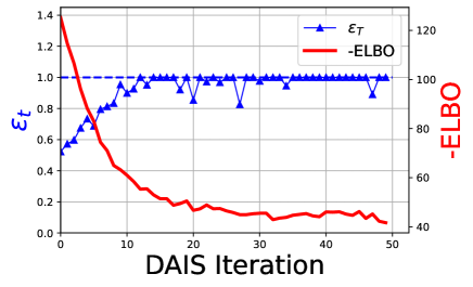
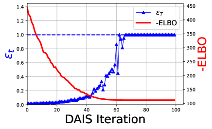
Figure 2: Tracking of the damping parameter $\varepsilon_{t}$ and (estimate of) the negative $\mathrm{ELBO}$ for monitoring convergence. (Left) $2$-dimensional target $\pi(x)\propto{\exp[-\{x_{2}-\mathcal{F}(x_{1})\}^{2}/(2\sigma^{2})]}\,p_{0}(x_{1},x_{2})$ with $\mathcal{F}(x)=1+\sin(2x)$ and $p_{0}(x_{1},x_{2})$ the density of a standard Gaussian density in $\mathbb{R}^{2}$. (Right) $d=100$ dimensional Gaussian target distribution with mean $\mu=(1,\ldots,1)\in\mathbb{R}^{d}$ and covariance $\Gamma_{i,j}=0.9+0.1\,\delta(i=j)$.

Figure 2 displays the trajectories of $t\mapsto\varepsilon_{t}$ and $t\mapsto-\widehat{\mathrm{ELBO}}(q_{t})$ when DAIS is used for approximating the following two target densities: (i) a $d=2$ dimensional density $\pi(x_{1},x_{2})$ defined as $\pi(x_{1},x_{2})/p_{0}(x_{0},x_{1})\propto{\exp[-\{x_{2}-\mathcal{F}(x_{1})\}^{2}/(2\sigma^{2})]}$ for $\sigma=0.1$, non-linear function $\mathcal{F}(x)=1+\sin(2x)$ and standard Gaussian prior density $p_{0}(x_{0},x_{1})$; (ii) a $d=100$ dimensional Gaussian distribution with mean $\mu=(1,\ldots,1)\in\mathbb{R}^{d}$ and covariance $\Gamma_{i,j}=0.9+0.1\,\delta(i=j)$. In both cases, DAIS is started from a standard multivariate Gaussian distribution, i.e. $\mu_{1}=0_{d\times 1}$ and $\Gamma_{1}=\mathrm{I}_{d}$. Figure 2 shows that monitoring either the damping parameter $\varepsilon_{t}\in(0,1]$ or the ELBO leads to roughly the same conclusion. In this paper, we monitor $\varepsilon_{t}$ as detailed in Appendix LABEL:ap:term_cond and use learning rate $\zeta_{t}=\varepsilon_{t}$. The resulting scheme is summarized in Algorithm 1.

Algorithm 1 Doubly adaptive importance sampling

1. Initialize the algorithm with $q_{1}\equiv\mathcal{N}(\mu_{1},\Gamma_{1})$.

2. For $t=1,2,\dots$ until $\varepsilon_{t}=1$ or some other stopping criterion:

   1. Sample $x_{s}\sim q_{t}\equiv\mathcal{N}\left(\mu_{t},\Gamma_{t}\right)$ independently for $s=1,\dots,S$.

   2. For a damping parameter $\varepsilon$, the unnormalized importance weights are:
      $w_{ts}(\varepsilon)=\exp\{\varepsilon\,\Phi_{t}(x_{s})\}$
      and the ESS is then:
      $\mathrm{ESS}_{t}(\varepsilon)=\{\sum_{s=1}^{S}w_{ts}(\varepsilon)\}^{2}/\sum_{s=1}^{S}w_{ts}^{2}(\varepsilon)$

      For a given threshold $1<N_{\text{ESS}}<S$, update the damping parameter $\varepsilon$:

      $\begin{array}[]{ll}\varepsilon_{t}=1,&\text{if }\;\mathrm{ESS}_{t}(1)\geq N_{\mathrm{ESS}}\\ \varepsilon_{t}=\max\left\{\varepsilon\in(0,1):\mathrm{ESS}_{t}(\varepsilon)\geq N_{\mathrm{ESS}}\right\},&\text{if }\;\mathrm{ESS}_{t}(1)<N_{\mathrm{ESS}}\end{array}$

   3. Compute $q_{t+1}\equiv\mathcal{N}(\mu_{t+1},\Gamma_{t+1})$ using the samples $x_{s}$ weighted by $w_{ts}(\varepsilon_{t})$:

      1. Set $\mu_{t+1}$ equal to an IS estimate of the right-hand side of (8a).

      2. Set $\Gamma_{t+1}$ equal to an IS estimate of the right-hand side of (8b).

3. Return the final Gaussian $q_{t+1}$ as the approximation to the target distribution $\pi$.

3 Related Work

We now provide an overview of existing posterior approximation approaches, in order to contextualise the proposed approach DAIS and highlight relevant connections.

3.1 Methods Based on Importance Sampling

We start by reviewing AIS (Bugallo et al., 2017) with Gaussian proposal distributions to approximate the target $\pi$. AIS is firstly initialized to $q_{1}$, a Gaussian distribution with mean $\mu_{1}$ and covariance $\Gamma_{1}$, for instance obtained from the prior distribution or from an initial approximation to the target $\pi$. Then, the proposal $q_{t+1}$ at each iteration is determined via the IS approximation to $\pi$ from the previous iteration. That is, $\mu_{t+1}$ and $\Gamma_{t+1}$ are chosen so that $q_{t+1}$ is closer to $\pi$, resulting in a more accurate IS approximation.

AIS (Bugallo et al., 2017) and DAIS iteratively improve $q_{t}$ via moment matching. A novelty of DAIS is in the choice of the new parameters $\mu_{t+1}$ and $\Gamma_{t+1}$ in (3), which is based on an application of Stein’s lemma. Another difference from previous AIS schemes is the adaptation of the IS target in the ultimate iteration to guarantee ESS. Elvira et al. (2015) propose an AIS approach that, like ours, uses the gradient of the target $\pi$. Though, their gradient appears due to gradient ascent while ours derives from moment matching with Stein’s lemma. Ryu and Boyd (2015) derive an AIS scheme via stochastic gradient descent on the MC error resulting from a proposal $q_{t}$. They use a single importance sample to move from $q_{t}$ to $q_{t+1}$ and then use all samples across iterations to estimate posterior quantities. In contrast, DAIS uses multiple samples but only from one iteration at a time.

Smoothing of IS weights, of which the damping in DAIS is a special case, has been employed in IS (e.g. Koblents and Míguez, 2013; Vehtari et al., 2024) and in AIS (Paananen et al., 2021). Most similarly to DAIS, Koblents and Míguez (2013) base their decision whether to temper the weights on ESS, though they do not adapt the amount of tempering to the target. Like DAIS but with a different smoothing method, Paananen et al. (2021) use a stopping criterion based on the regularity of the weights to determine the number of AIS iterations. Their proposal distributions, arising from specific tasks such as Bayesian cross-validation, are complicated while DAIS considers Gaussian proposals with a focus on approximating the posterior mean and covariance of the target distribution.

Similarly to DAIS, SMC (Del Moral et al., 2006) and annealed IS (Neal, 2001) adapt the target and proposal across iterations. Moreover, automatic tempering using ESS is also used in adaptive SMC (e.g. Chopin and Papaspiliopoulos, 2020, Algorithm 17.3). In these methods, proposals are discrete distributions based on reweighted, resampled or rejuvenated particles while DAIS adapts a Gaussian proposal.

3.2 Optimization-based Methods

Moment matching is fundamental to EP (Minka, 2001) and expectation consistent approximate inference (Opper and Winther, 2005). These methods usually entail such matching iteratively across factors of the target density $\pi$. That is, expectations are propagated across a Bayesian network. This contrasts with our matching, which uses all of $\pi$ at once, e.g. $\mu_{t+1}=\mathbb{E}_{q_{t,\varepsilon_{t}}}[X]$. Disregarding this discrepancy, the damped moment matching of DAIS is equivalent to damping in EP (Vehtari et al., 2020, Section 5.2) and to the $\alpha$-divergence minimization scheme in Equation (18) of Minka (2005). Like DAIS, the EP methods by Wiegerinck and Heskes (2003), Minka (2004) and Hernández-Lobato et al. (2016) minimize the $\alpha$-divergence. The updates in (3) involve taking the expectation, or smoothing, of gradients. Dehaene (2016) links smoothed gradients to EP and minimization of $\alpha$-divergence.

Prangle and Viscardi (2022) consider the same damped target $q_{t,\varepsilon_{t}}$, also based on ESS, while iteratively updating an IS proposal $q_{t}$ as in DAIS. Differences include that $q_{t}$ is not a Gaussian distribution but a normalizing flow and that $q_{t}$ is updated via gradient descent for the objective $\mathrm{KL}{\left(\,q_{t,\varepsilon_{t}}\,\|\,q_{t+1}\,\right)}$. DAIS updates $q_{t}$ through moment matching, e.g. $\mu_{t+1}=\mathbb{E}_{q_{t,\varepsilon_{t}}}[X]$, which directly targets the minimizer of $\mathrm{KL}{\left(\,q_{t,\varepsilon_{t}}\,\|\,q_{t+1}\,\right)}$.

There is a VI literature on improving variational objectives and approximating families via MC (e.g. Li and Turner, 2016; Ruiz and Titsias, 2019) including IS (e.g. Domke and Sheldon, 2018; Wang et al., 2018) and AIS (Han and Liu, 2017; Jerfel et al., 2021). DAIS constitutes a substantially different hybrid between VI and MC as it performs AIS that happens to recover natural-gradient VI via damping as $\varepsilon_{t}\to 0$ (see Section 4). Some VI methods (e.g. Li and Turner, 2016) replace the reverse KL divergence by $\alpha$-divergence, which DAIS effectively also minimizes (see Section 4). Importantly, DAIS, derived as AIS instead of a change in VI objective, yields principled adaption of $\alpha=\varepsilon_{t}$. In this context, Wang et al. (2018) consider adaptation of the divergence based on tail probabilities of importance weights. Yao et al. (2018) evaluate the accuracy of VI using IS. Liu and Wang (2016) use Stein’s lemma for VI. They minimize the reverse KL divergence via a functional gradient descent derived from the Stein discrepancy. Han and Liu (2017) expand that Stein VI method to use AIS.

As in DAIS, recent works by Modi et al. (2023) and Cai et al. (2024) propose an alternative VI approach where, under a Gaussian $q_{t}$, variational parameters are updated using closed-form equations suitable for handling full covariance matrices. In particular, the approach by Modi et al. (2023) is based on the minimization of the forward KL divergence under the additional constraint of score matching (i.e. the matching of the gradient of the logarithm of the variational density to the target), while Cai et al. (2024) minimize a score-based divergence. Cai et al. (2024) show how the first approach can be recovered as limiting case of the second one. In contrast to DAIS, these methods do not control MC error.

4 Analysis of DAIS

Implementing the DAIS algorithm with learning rate $\zeta_{t}=\varepsilon_{t}$ corresponds to iteratively matching, up to MC variability, the first two moments of the damped target density $q_{t,\varepsilon}$ to the ones of the next Gaussian approximation $q_{t+1}$. This demonstrates that the algorithm does not depend on the mean-covariance parametrization of the Gaussian family, and that any other parametrization would lead to exactly the same sequence of Gaussian approximations. This remark motivates the connections described in this section between the proposed DAIS algorithm and the natural-gradient descent method (Amari, 1998).

While the standard gradient is the steepest descent direction when the usual Euclidean distance is used, the natural gradient is the steepest descent direction in the space of distributions where distance is measured by the KL divergence (Martens, 2020). In particular, natural-gradient flows are parametrization invariant. In the Gaussian setting of this article, the natural-gradient flow for minimizing a loss function $\mathcal{L}(\mu,\Gamma)$ over the space of Gaussian distributions $q\in\mathcal{Q}_{\mathrm{gauss}}$ is

$$\left\{\begin{aligned} \frac{d\mu}{dt}&=-\Gamma\,\nabla_{\mu}\mathcal{L}\\ \frac{d\Gamma^{-1}}{dt}&=2\,\nabla_{\Gamma}\mathcal{L}\\ \end{aligned}\right.\qquad\Longleftrightarrow\qquad\left\{\begin{aligned} \frac{d\mu}{dt}&=-\Gamma\,\nabla_{\!\mu}\mathcal{L}\equiv-\widetilde{\nabla}_{\!\mu}\mathcal{L}\\ \frac{d\Gamma}{dt}&=-2\,\Gamma{\left(\nabla_{\Gamma}\mathcal{L}\right)}\Gamma\equiv-\widetilde{\nabla}_{\Gamma}\mathcal{L},\end{aligned}\right.$$ (10)

where $\widetilde{\nabla}_{\mu}\mathcal{L}=\Gamma\,\nabla_{\mu}\mathcal{L}$ and $\widetilde{\nabla}_{\Gamma}\mathcal{L}=2\,\Gamma{\left(\nabla_{\Gamma}\mathcal{L}\right)}\Gamma$ denote the natural gradient with respect to the mean and covariance parameters, respectively. A derivation of (10) can be found in Khan et al. (2017) and the equivalence between these two formulations follows from the chain rule. Since $\nabla_{\Gamma}\mathbb{E}_{q}[\varphi(X)]=\tfrac{1}{2}\,\mathbb{E}_{q}[\nabla_{xx}\varphi(X)]$ for any test function $\varphi:\mathbb{R}^{d}\to\mathbb{R}$ (Opper and Archambeau, 2009, Equation (A.3)), standard algebraic manipulations show that the forward (Fwd) and reverse (Rev) KL divergences satisfy:

$$\textrm{(Rev)}: \left\{\begin{aligned} \nabla_{\mu}\mathrm{KL}{\left(\,q\,\|\,\pi\,\right)}&=-\mathbb{E}_{q}[\nabla_{x}\log\pi(X)]\\ \nabla_{\Gamma}\mathrm{KL}{\left(\,q\,\|\,\pi\,\right)}&=\frac{1}{2}\left(-\mathbb{E}_{q}[\nabla^{2}_{xx}\log\pi(X)]-\Gamma^{-1}\right)\end{aligned}\right.$$ (11)

$$\textrm{(Fwd)}: \left\{\begin{aligned} \nabla_{\mu}\mathrm{KL}{\left(\,\pi\,\|\,q\,\right)}&=-\Gamma^{-1}\,\mathbb{E}_{\pi}[(X-\mu)]\\ \nabla_{\Gamma}\mathrm{KL}{\left(\,\pi\,\|\,q\,\right)}&=-\frac{1}{2}\,\mathbb{E}_{\pi}[\Gamma^{-1}(X-\mu)\otimes(X-\mu)\Gamma^{-1}-\Gamma^{-1}].\end{aligned}\right.$$ (12)

It follows that the natural-gradient flow for minimizing the forward and reverse KL divergences are given by

$$\textrm{(Rev)}:\left\{\begin{aligned} \frac{d\mu}{dt}&=\Gamma\,\mathbb{E}_{q}[\nabla_{x}\log\pi(X)]\\ \frac{d\Gamma}{dt}&=\Gamma\,\mathbb{E}_{q}[\nabla^{2}_{xx}\log\pi(X)]\,\Gamma+\Gamma\end{aligned}\right.\qquad\textrm{(Fwd)}:\left\{\begin{aligned} \frac{d\mu}{dt}&=\mathbb{E}_{\pi}[(X-\mu)]\\ \frac{d\Gamma}{dt}&=\mathbb{E}_{\pi}[(X-\mu)\otimes(X-\mu)]-\Gamma.\end{aligned}\right.$$ (13)

Since $q_{t,\varepsilon_{t}}$ converges to $q_{t}=\mathcal{N}(\mu,\Gamma)$ as $\varepsilon_{t}\to 0$ and $\nabla\Phi_{t}(x)=\nabla\log\pi(x)+\Gamma^{-1}(x-\mu)$, the quantities $\mathbf{G}_{\mu}(q_{t},\varepsilon_{t})=\mathbb{E}_{q_{t,\varepsilon_{t}}}[\Gamma\,\nabla\Phi_{t}(X)]$ and $\mathbf{G}_{\Gamma}(q_{t},\varepsilon_{t})=\mathrm{cov}_{q_{t,\varepsilon_{t}}}[\Gamma\,\nabla\Phi_{t}(X),X]$ defined in (3) satisfy

$$\left\{\begin{aligned} \lim_{\varepsilon_{t}\to 0}\mathbf{G}_{\mu}(q_{t},\varepsilon_{t})&=\Gamma\mathbb{E}_{q_{t}}[\,\nabla_{x}\log\pi(X)]=-\widetilde{\nabla}_{\mu}\mathrm{KL}{\left(\,q_{t}\,\|\,\pi\,\right)}\\ \lim_{\varepsilon_{t}\to 0}\mathbf{G}_{\Gamma}(q_{t},\varepsilon_{t})&=\Gamma\,\mathbb{E}_{q_{t}}[\nabla^{2}_{xx}\log\pi(X)]\,\Gamma+\Gamma=-\widetilde{\nabla}_{\Gamma}\mathrm{KL}{\left(\,q_{t}\,\|\,\pi\,\right)}.\end{aligned}\right.$$ (14)

The second equality follows from an integration by parts (or Stein’s lemma). Equation (14) shows that, in the limit of small damping parameter $\varepsilon_{t}\to 0$, the DAIS method can be understood as a natural-gradient descent for minimizing the reverse KL divergence. Furthermore, since $q_{t,\varepsilon_{t}}$ converges to $\pi$ as $\varepsilon_{t}\to 1$, the definitions $\mu_{t,\varepsilon_{t}}=\mu_{t}+\varepsilon_{t}\,\mathbf{G}_{\mu}(q_{t},\varepsilon_{t})$ and $\Gamma_{t,\varepsilon_{t}}=\Gamma_{t}+\varepsilon_{t}\,\mathbf{G}_{\Gamma}(q_{t},\varepsilon_{t})$ show that

$$\left\{\begin{aligned} \lim_{\varepsilon_{t}\to 1}\mathbf{G}_{\mu}(q_{t},\varepsilon_{t})&=\mu_{\pi}-\mu=-\widetilde{\nabla}_{\mu}\mathrm{KL}{\left(\,\pi\,\|\,q_{t}\,\right)}\\ \lim_{\varepsilon_{t}\to 1}\mathbf{G}_{\Gamma}(q_{t},\varepsilon_{t})&=\Gamma_{\pi}-\Gamma=-\widetilde{\nabla}_{\Gamma}\mathrm{KL}{\left(\,\pi\,\|\,q_{t}\,\right)}-(\mu_{\pi}-\mu)\otimes(\mu_{\pi}-\mu)\end{aligned}\right.$$ (15)

where $\mu_{\pi}=\mathbb{E}_{\pi}[X]$ and $\Gamma_{\pi}=\mathrm{cov}_{\pi}(X,X)$. Equation (15) establishes a connection between DAIS and the natural-gradient flow for minimizing the forward KL, whose global minimizer is indeed given by the Gaussian distribution with first two moments matching those of the target distribution $\pi$.

To conclude this section, we characterize the limiting distribution obtained by the DAIS methodology. For this purpose, assume that the DAIS algorithm has converged towards an approximating distribution $q_{\infty}=\mathcal{N}(\mu_{\infty},\Gamma_{\infty})$ with final damping parameter $0<\varepsilon_{\infty}<1$. The moment matching conditions mean that

$$\mathbb{E}_{q_{\infty}}[T(X)]\;=\;\mathbb{E}_{q_{\infty,\varepsilon_{\infty}}}[T(X)]$$ (16)

where $q_{\infty,\varepsilon_{\infty}}(x)\propto q_{\infty}^{1-\varepsilon_{\infty}}(x)\,\pi^{\varepsilon_{\infty}}(x)$. In the identity above, $T:\mathbb{R}^{d}\to\mathbb{R}^{d+d(d+1)/2}$ equals $T(x)=(x_{i},x_{i}x_{j})_{i\leq j}$, representing the sufficient statistic vector for a $d$-dimensional Gaussian distribution in its natural parametrization. Recall that the Gaussian family can be parametrized as $q_{\lambda}(x)=\exp(\left<\lambda,T(x)\right>)/Z(\lambda)$ for natural parameter $\lambda\in\Lambda\subset\mathbb{R}^{d+d(d+1)/2}$ and associated normalizing constant $Z(\lambda)>0$. We remark that the following can be generalized to any natural exponential family. Condition (16) describes the stationary points of the $\alpha$-divergence functional $\lambda\mapsto\mathrm{K}_{\alpha}{\left(\,\pi\,\|\,q_{\lambda}\,\right)}$ (Hernández-Lobato et al., 2016) which Amari (1985) defines as

$$\mathrm{K}_{\alpha}{\left(\,\pi\,\|\,q_{\lambda}\,\right)}=\frac{1}{\alpha(1-\alpha)}{\left[1-\int_{\mathcal{X}}{\left\{\frac{d\pi}{dq_{\lambda}}(x)\right\}}^{\alpha}q_{\lambda}(dx)\right]}$$ (17)

The result follows by showing that

$$\nabla_{\lambda}\mathrm{K}_{\alpha}{\left(\,\pi\,\|\,q_{\lambda}\,\right)}=\frac{Z(\lambda,\alpha)}{\alpha}{\left(\mathbb{E}_{q_{\lambda,\alpha}}[T(X)]-\mathbb{E}_{q_{\lambda}}[T(X)]\right)}$$ (18)

where $Z(\lambda,\alpha)=\int\pi(x)^{\alpha}\,q^{1-\alpha}_{\lambda}(x)\,dx$. Consequently, (16) shows that the limiting Gaussian distribution $q_{\infty}$ is a stationary point of the $\alpha$-divergence functional $\lambda\mapsto\mathrm{K}_{\alpha}{\left(\,\pi\,\|\,q_{\lambda}\,\right)}$ when choosing $\alpha=\varepsilon_{\infty}$. Since $\mathrm{K}_{\alpha}{\left(\,\pi\,\|\,q\,\right)}\to\mathrm{KL}{\left(\,\pi\,\|\,q\,\right)}$ as $\alpha\to 1$ and $\mathrm{K}_{\alpha}{\left(\,\pi\,\|\,q\,\right)}\to\mathrm{KL}{\left(\,\pi\,\|\,q\,\right)}$ as $\alpha\to 0$, this result further indicates that large update parameters $\varepsilon_{t}$ are to be favoured since minimizing $\mathrm{KL}{\left(\,\pi\,\|\,q_{t}\,\right)}$ is preferred over minimizing $\mathrm{KL}{\left(\,q_{t}\,\|\,\pi\,\right)}$.

5 Applications

This section compares the performance of DAIS with other approximations. Additionally, Appendix LABEL:ap:inverse considers an inverse problem where, without any problem-specific adjustments or reduced approximation accuracy, DAIS is faster than an approximation that exploits the structure of the problem. We use the Python package JAX (Bradbury et al., 2018) for automatic differentiation to obtain $\nabla\!_{x}\Phi_{t}(x)$ and for parallelization of importance samples across 32 CPU cores.

5.1 Two-dimensional Synthetic Examples

As a first example, we consider two bivariate distributions from Ruiz and Titsias (2019) as their low dimensionality allows for easy inspection of approximations. Specifically, we consider the banana-shaped target distribution

$$\pi(x)\propto\mathcal{N}{\left\{\begin{pmatrix}x_{1}\\ x_{2}+x_{1}^{2}+1\end{pmatrix}\middle|\ 0,\begin{pmatrix}1&0.9\\ 0.9&1\end{pmatrix}\right\}}$$ (19)

and the mixture of two Gaussian distributions

$$\pi(x)=0.3\,\mathcal{N}{\left\{x\,\middle|\ \begin{pmatrix}0.8\\ 0.8\end{pmatrix},\begin{pmatrix}1&0.8\\ 0.8&1\end{pmatrix}\right\}}+0.7\,\mathcal{N}{\left\{x\,\middle|\ \begin{pmatrix}-2\\ -2\end{pmatrix},\begin{pmatrix}1&-0.6\\ -0.6&1\end{pmatrix}\right\}}$$ (20)

visualised in Figure 3.

Figure 3: The banana-shaped and mixture densities in greyscale with mean (dot) and 95% credible regions (ellipse) of the corresponding Gaussian approximations overlaid. The Gaussian approximations have their moments equal to the exact moments (black, dotted), the DAIS estimates (blue, solid) and the VI estimates (red, dashed).

We approximate these distributions using Gaussian proposals. As a baseline Gaussian approximation, we compute the exact mean and covariance by numerical integration. Algorithm 1 provides an approximation with importance sample size $S=10^{5}$ and $N_{\mathrm{ESS}}=10^{3}$. With these values, DAIS finishes with $\varepsilon_{t}=1$ in 3 and 2 iterations for the banana-shaped and the mixture distribution, respectively. Appendix LABEL:ap:2D_eps considers a lower sample size $S$ resulting in a final $\varepsilon_{t}$ less than one. For comparison, we run VI with the same full covariance Gaussian distribution as DAIS uses. Specifically, we minimize the reverse KL divergence $\mathrm{KL}{\left(\,q_{t}\,\|\,\pi\,\right)}$ via gradient descent.

Figure 3 summarizes the results. DAIS captures the mean and covariance of the target distribution $\pi$ more accurately than VI. In particular, the DAIS approximation for the mixture distribution is virtually indistinguishable from the exact mean and covariance. This shows the benefit of minimizing $\mathrm{KL}{\left(\,\pi\,\|\,q_{t}\,\right)}$ instead of $\mathrm{KL}{\left(\,q_{t}\,\|\,\pi\,\right)}$. The covariance underestimation by DAIS for the banana-shaped distribution is likely due to the ESS estimator in Step 2b of Algorithm 1 underestimating MC error (Elvira et al., 2022). Additionally, the results in Appendix LABEL:ap:2D_eps where $\varepsilon_{t}<1$ are in line with the fact that the adaptation of $\varepsilon_{t}$ interpolates between moment matching and VI.

5.2 Logistic Regression

Lastly, we apply DAIS to the four logistic regression examples from Section 4.2.1 of Ong et al. (2018). Each data set consists of a binary response $y_{i}\in\{-1,1\}$ and a $d$-dimensional feature vector $a_{i}\in\mathbb{R}^{d}$ for $1\leq i\leq n$ where $n$ is the number of cases. Then, the likelihood is $\ell(y\!\mid\!x)=\prod_{i=1}^{n}1/\{1+\exp(-y_{i}\left<a_{i},x\right>)\}$ where $x$ is the coefficient vector. The prior on $x$ is $p_{0}=\mathcal{N}(0,10\,\mathrm{I}_{d})$ such that the posterior follows as $\pi(x)\propto\mathcal{N}\left(x\!\mid\!0,10\,\mathrm{I}_{d}\right)\ell(y\!\mid\!x)$.

The data involved are binarized versions of the spam, krkp, ionosphere and mushroom data from the UCI Machine Learning Repository (Dua and Graff, 2017). The binarization follows Gelman et al. (2008, Section 5.1). First, any continuous attributes are discretized using the method from Fayyad and Irani (1993). Then, the resulting set of categorical attributes are encoded using dummy variables with the most frequent category as baseline. These dummy variables plus an intercept constitute the $d$ predictors considered. The resulting problem dimensionalities are summarized in Table 1.

Table 1: Number of cases, number of categorical and continuous attributes, resulting number of predictors $d$, importance sample size $S$, number of iterations and computation time in seconds of DAIS for the logistic regression examples.

Data name	Cases	Categorical	Continuous	$d$	$S$	Iterations	Time
Spam	4,601	57	0	105	$10^{4}$	4	11s
Krkp	3,196	0	36	38	$2\cdot 10^{3}$	3	5.8s
Ionosphere	351	32	0	111	$5\cdot 10^{5}$	6	170s
Mushroom	8,124	0	22	96	$2\cdot 10^{5}$	8	319s

Algorithm 1 with $N_{\mathrm{ESS}}=10^{3}$ approximates the mean and covariance of $\pi$. The posterior mode $\mu_{1}=\arg\max_{x}\pi(x)$ and the inverse Hessian of the negative log-density $\Gamma_{1}=\{-\nabla^{2}U(\mu_{1})\}^{-1}$ provide the initial approximation $q_{1}=\mathcal{N}(\mu_{1},\Gamma_{1})$. Importance sample sizes $S$ are as in Table 1. They are chosen to ensure that DAIS ultimately needs no damping ($\varepsilon_{t}=1$). Table 1 also lists computation times and number of DAIS iterations. The computation times refer to wall time or actual time. The total CPU time, which is the sum of the times spent on DAIS by each CPU core, is higher due to parallelization. The relative difference is most extreme for the mushroom data which took 5 minutes while CPU time was 1 hour. To assess approximation accuracy, we run Hamiltonian MC using the Python package Mici (Graham, 2020) for 100,000 iterations, of which 10,000 are burn-in iterations.

Figure 4: Scatter plots of the DAIS estimates versus the Hamiltonian MC estimates of the posterior means and standard deviations for the logistic regression examples.

Figure 4 shows that DAIS provides highly accurate estimates of posterior moments. In general, the DAIS estimates are more accurate than those from mean-field VI in Figure LABEL:fig:uci_VI in Supplementary Material and doubly stochastic VI (Titsias and Lázaro-Gredilla, 2014) as shown in Figure 6 of Ong et al. (2018). To explore the effect of reduced MC error from (8) on the approximation of $\pi$, Figure LABEL:fig:uci_no_Stein in Supplementary Material is the same as Figure 4 except that it does not use (8). Comparing these figures reveals that (8) indeed improves approximation accuracy.

6 Discussion

We propose a novel iterative approach to the approximation of the posterior distribution in general Bayesian models. The methodology is based on producing a sequence of Gaussian distributions whose moments match those of a damped target distribution, thus adapting to the target. This sequence is identified by exploiting Stein’s lemma, which provides an updating rule for two consecutive sets of moments. The moments are computed via importance sampling while damping of the target is used to control the effective sample size (ESS) of the samples in the importance sampling. The adaptation guarantees that the ESS is above a pre-specified threshold, which controls MC error, and provides a trade-off between minimizing the reverse and forward KL divergences based on computational constraints. We call the method doubly adaptive importance sampling (DAIS). DAIS is a general methodology and competitive with methods that are more tailored to a problem-specific posterior.

DAIS inherits certain limitations from IS. Firstly, high dimensionality typically results in too low ESS for IS to be feasible and translates to exceedingly high damping in DAIS. Also, a large number of samples $S$ requires considerable computer memory. Additionally, the Gaussianity of the proposals $q_{t}$ limits how accurately DAIS can approximate the target $\pi$. To go beyond this limitation, $\pi$ can be approximated by the importance-weighted samples from the last iteration of DAIS. The approximation can be made arbitrarily accurate by increasing the number of samples $S$ in this last iteration. Additionally, importance weights from multiple iterations of DAIS can be combined to approximate $\pi$ as in Equation (17) of Bugallo et al. (2017), especially if the amount of damping $\varepsilon_{t}$ is nearly constant over these iterations.

Another avenue for increasing accuracy is going beyond Gaussianity for $q_{t}$. The Gaussian constraint enables the MC error reduction in (8). Other aspects of DAIS such as its adaptation and the analysis in Section 4 do not require Gaussianity. Moreover, Lin et al. (2019) extend Stein’s lemma beyond Gaussian distributions to mixtures of an exponential family, potentially enabling MC error reduction similar to (8) for more general $q_{t}$. As such, ideas behind DAIS can be used with non-Gaussian approximating distributions.

SUPPLEMENTARY MATERIAL

Supplement:

Derivation of Equation (8), discussion of the stopping criterion used in Algorithm 1 and additional empirical results. (.pdf file)

Code:

Scripts that produce the empirical results are available at https://github.com/thiery-lab/dais. (GitHub repository)

References

- Amari (1985) Amari, S. (1985). Differential-Geometrical Methods in Statistics. Lecture Notes in Statistics. New York, NY: Springer. Chapter 3.
- Amari (1998) Amari, S. (1998). Natural gradient works efficiently in learning. Neural Computation 10(2), 251–276.
- Beskos et al. (2016) Beskos, A., A. Jasra, N. Kantas, and A. Thiery (2016). On the convergence of adaptive sequential Monte Carlo methods. The Annals of Applied Probability 26(2), 1111–1146.
- Blei et al. (2017) Blei, D. M., A. Kucukelbir, and J. D. McAuliffe (2017). Variational inference: A review for statisticians. Journal of the American Statistical Association 112(518), 859–877.
- Bradbury et al. (2018) Bradbury, J., R. Frostig, P. Hawkins, M. J. Johnson, C. Leary, D. Maclaurin, and S. Wanderman-Milne (2018). JAX: composable transformations of Python+NumPy programs. http://github.com/google/jax.
- Bugallo et al. (2017) Bugallo, M. F., V. Elvira, L. Martino, D. Luengo, J. Miguez, and P. M. Djuric (2017). Adaptive importance sampling: The past, the present, and the future. IEEE Signal Processing Magazine 34(4), 60–79.
- Cai et al. (2024) Cai, D., C. Modi, L. Pillaud-Vivien, C. C. Margossian, R. M. Gower, D. M. Blei, and L. K. Saul (2024). Batch and match: black-box variational inference with a score-based divergence. arXiv:2402.14758v1.
- Chopin and Papaspiliopoulos (2020) Chopin, N. and O. Papaspiliopoulos (2020). An Introduction to Sequential Monte Carlo. Springer Series in Statistics. Springer Nature Switzerland.
- Dehaene (2016) Dehaene, G. P. (2016). Expectation propagation performs a smoothed gradient descent. arXiv:1612.05053v1.
- Del Moral et al. (2006) Del Moral, P., A. Doucet, and A. Jasra (2006). Sequential Monte Carlo samplers. Journal of the Royal Statistical Society: Series B (Statistical Methodology) 68(3), 411–436.
- Domke and Sheldon (2018) Domke, J. and D. R. Sheldon (2018). Importance weighting and variational inference. In Advances in Neural Information Processing Systems, Volume 31. Curran Associates, Inc.
- Dua and Graff (2017) Dua, D. and C. Graff (2017). UCI Machine Learning Repository. University of California, Irvine, School of Information and Computer Sciences, http://archive.ics.uci.edu/ml.
- Elvira et al. (2015) Elvira, V., L. Martino, D. Luengo, and J. Corander (2015). A gradient adaptive population importance sampler. In 2015 IEEE International Conference on Acoustics, Speech and Signal Processing (ICASSP), pp. 4075–4079. IEEE.
- Elvira et al. (2022) Elvira, V., L. Martino, and C. P. Robert (2022). Rethinking the effective sample size. International Statistical Review 90(3), 525–550.
- Fayyad and Irani (1993) Fayyad, U. M. and K. B. Irani (1993). Multi-interval discretization of continuous-valued attributes for classification learning. In Proceedings of the Thirteenth International Joint Conference on Artificial Intelligence, Vol. 2, pp. 1022–1027.
- Gelman et al. (2008) Gelman, A., A. Jakulin, M. G. Pittau, and Y. Su (2008). A weakly informative default prior distribution for logistic and other regression models. The Annals of Applied Statistics 2(4), 1360–1383.
- Graham (2020) Graham, M. M. (2020). Mici: Manifold Markov chain Monte Carlo methods in Python. https://github.com/matt-graham/mici.
- Han and Liu (2017) Han, J. and Q. Liu (2017). Stein variational adaptive importance sampling. In Proceedings of the Thirty-Third Conference on Uncertainty in Artificial Intelligence, UAI 2017, Sydney, Australia, August 11-15, 2017. AUAI Press.
- Hernández-Lobato et al. (2016) Hernández-Lobato, J., Y. Li, M. Rowland, T. Bui, D. Hernández-Lobato, and R. Turner (2016). Black-box -divergence minimization. In Proceedings of The 33rd International Conference on Machine Learning, Volume 48 of Proceedings of Machine Learning Research, New York, NY, pp. 1511–1520. PMLR.
- Jerfel et al. (2021) Jerfel, G., S. Wang, C. Wong-Fannjiang, K. A. Heller, Y. Ma, and M. I. Jordan (2021). Variational refinement for importance sampling using the forward Kullback-Leibler divergence. In Proceedings of the Thirty-Seventh Conference on Uncertainty in Artificial Intelligence, Volume 161 of Proceedings of Machine Learning Research, pp. 1819–1829. PMLR.
- Khan et al. (2017) Khan, M. E., W. Lin, V. Tangkaratt, Z. Liu, and D. Nielsen (2017). Variational adaptive-Newton method for explorative learning. In Advances in Approximate Bayesian Inference. NIPS 2017 Workshop.
- Khan and Nielsen (2018) Khan, M. E. and D. Nielsen (2018). Fast yet simple natural-gradient descent for variational inference in complex models. In 2018 International Symposium on Information Theory and Its Applications (ISITA), pp. 31–35. IEEE.
- Koblents and Míguez (2013) Koblents, E. and J. Míguez (2013). A population Monte Carlo scheme with transformed weights and its application to stochastic kinetic models. Statistics and Computing 25(2), 407–425.
- Li and Turner (2016) Li, Y. and R. E. Turner (2016). Rényi divergence variational inference. In Advances in Neural Information Processing Systems, Volume 29. Curran Associates, Inc.
- Lin et al. (2019) Lin, W., M. E. Khan, and M. Schmidt (2019). Stein’s lemma for the reparameterization trick with exponential family mixtures. arXiv:1910.13398v1.
- Liu and Wang (2016) Liu, Q. and D. Wang (2016). Stein variational gradient descent: A general purpose Bayesian inference algorithm. In Advances in Neural Information Processing Systems 29. Curran Associates, Inc.
- Martens (2020) Martens, J. (2020). New insights and perspectives on the natural gradient method. Journal of Machine Learning Research 21, 146.
- Minka (2004) Minka, T. (2004). Power EP. Technical Report MSR-TR-2004-149, Microsoft Research Ltd., Cambridge, UK.
- Minka (2005) Minka, T. (2005). Divergence measures and message passing. Technical Report MSR-TR-2005-173, Microsoft Research Ltd., Cambridge, UK.
- Minka (2001) Minka, T. P. (2001). Expectation propagation for approximate Bayesian inference. In Proceedings of the Seventeenth Conference on Uncertainty in Artificial Intelligence, pp. 362–369.
- Mira et al. (2013) Mira, A., R. Solgi, and D. Imparato (2013). Zero variance Markov chain Monte Carlo for Bayesian estimators. Statistics and Computing 23(5), 653–662.
- Modi et al. (2023) Modi, C., R. Gower, C. Margossian, Y. Yao, D. Blei, and L. Saul (2023). Variational inference with Gaussian score matching. In Advances in Neural Information Processing Systems 36. Curran Associates, Inc.
- Neal (2001) Neal, R. M. (2001). Annealed importance sampling. Statistics and Computing 11(2), 125–139.
- Oates et al. (2017) Oates, C. J., M. Girolami, and N. Chopin (2017). Control functionals for Monte Carlo integration. Journal of the Royal Statistical Society: Series B (Statistical Methodology) 79(3), 695–718.
- Ong et al. (2018) Ong, V. M.-H., D. J. Nott, and M. S. Smith (2018). Gaussian variational approximation with a factor covariance structure. Journal of Computational and Graphical Statistics 27(3), 465–478.
- Opper and Archambeau (2009) Opper, M. and C. Archambeau (2009). The variational Gaussian approximation revisited. Neural Computation 21(3), 786–792.
- Opper and Winther (2005) Opper, M. and O. Winther (2005). Expectation consistent approximate inference. Journal of Machine Learning Research 6, 2177–2204.
- Owen (2013) Owen, A. B. (2013). Monte Carlo Theory, Methods and Examples. https://artowen.su.domains/mc/.
- Paananen et al. (2021) Paananen, T., J. Piironen, P.-C. Bürkner, and A. Vehtari (2021). Implicitly adaptive importance sampling. Statistics and Computing 31(2), 16.