General Approach on Shadow Radius and Photon Spheres in Asymptotically Flat Spacetimes and the Impact of Mass-Dependent Variations
Abstract
Recent observations of black hole shadows have revolutionized our ability to probe gravity in extreme environments. This manuscript presents a novel analytic method to calculate, in leading-order terms, the key parameters of photon sphere and shadow radius. This method offers advantages for complex metrics where traditional approaches are cumbersome. We further explore the impact of black hole mass on the photon sphere radius, providing insights into black hole interactions with their surroundings. Our findings contribute significantly to black hole physics and gravity under extreme conditions. By leveraging future advancements in observations, such as the next-generation Event Horizon Telescope (ngEHT), this work paves the way for even more precise tests of gravity near black holes.
pacs:
95.30.Sf, 04.70.-s, 97.60.Lf, 04.50.KdI INTRODUCTION
The groundbreaking observations of black hole shadows have ushered in a new era for probing gravity in extreme environments. In the 1970s, physicist James Bardeen introduced the idea of a black hole shadow, which has since become a major focus in astrophysics research Bardeen (1968). This shadow forms because light bends around the black hole, creating a dark area against the background of bright surrounding matter Luminet (1979); Falcke et al. (2000). By studying this shadow, scientists can learn more about black holes, including their mass, spin, and the structure of spacetime nearby. Recent advances in observation, like very-long-baseline interferometry (VLBI) and the Event Horizon Telescope (EHT), have enabled direct imaging of the shadow of the supermassive black holes at the center of the M87 and and Sgr A* galaxies Akiyama et al. (2019, 2022). This has opened up new opportunities to test theories about gravity and the nature of black holes Bronzwaer and Falcke (2021); Vagnozzi et al. (2023); Vertogradov and Övgün (2024); Perlick et al. (2015); Virbhadra (2024); Adler and Virbhadra (2022); Virbhadra (2022); Virbhadra and Keeton (2008); Virbhadra and Ellis (2000); Virbhadra et al. (1998); Yang et al. (2024); Zakharov (2022, 2023); Alloqulov et al. (2024); Abdujabbarov et al. (2016); Atamurotov et al. (2013); Abdujabbarov et al. (2015); Abdikamalov et al. (2019); Abdujabbarov et al. (2015); Vagnozzi et al. (2020); Claudel et al. (2001); Hod (2020, 2013a, 2013b, 2023a, 2023b); Khoo and Ong (2016); Decanini et al. (2010); Pantig et al. (2022); Shoom (2017); Konoplya and Zhidenko (2021); Kuang and Övgün (2022); Bronnikov et al. (2021); Paithankar and Kolekar (2023); Konoplya et al. (2016); Johannsen and Psaltis (2011); Cardoso et al. (2014); Konoplya and Zhidenko (2019); Qiao (2022); Kokkotas et al. (2017); Hennigar et al. (2018); Konoplya et al. (2020); Aratore et al. (2024); Tsupko (2022); Cederbaum and Galloway (2016); Johannsen (2013); Teo (2003); Okyay and Övgün (2022); Lu and Lyu (2020); Younsi et al. (2016); Tsupko and Bisnovatyi-Kogan (2020); Tsukamoto et al. (2014); Ghosh et al. (2023); Övgün et al. (2024); Adair et al. (2020); Tsukamoto (2018); Gómez and Valageas (2024); Shaikh et al. (2019); Lambiase et al. (2023); Karshiboev et al. (2024); Rayimbaev et al. (2023); Mustafa et al. (2022); Pantig et al. (2023); Pantig and Övgün (2023); Kumaran and Övgün (2023); Çimdiker et al. (2023); Puliçe et al. (2023); Övgün et al. (2018); Heydarzade and Vertogradov (2023); Allahyari et al. (2020); Pedrotti and Vagnozzi (2024).
While General Relativity (GR) has successfully described many astronomical observations with high precision, there are compelling reasons to consider extending this framework. The theory has faced challenges in predicting phenomena such as the accelerating expansion of the Universe, the existence of dark matter, and its compatibility with quantum field theory. On the other hand, the direct observation of supermassive black holes offers a unique opportunity to test and constrain modifications to GR in their vicinity. Future projects like the Next Generation Event Horizon Telescope (ngEHT), which plans to incorporate satellites to increase baseline and image resolution, will provide even more precise measurements of supermassive black holes properties Tiede et al. (2022); Ayzenberg et al. (2023), such as spin. These observations will be crucial for testing alternative theories of gravity and improving our understanding of the fundamental forces governing the universe.
The photon sphere, also referred to as the circular photon orbit or light ring, and the shadow radius play crucial roles in the field of black hole physics Perlick and Tsupko (2022). These quantities are central to the examination of particle trajectories, gravitational lensing effects Ishihara et al. (2016); Kudo and Asada (2022), and optical phenomena related to black holes. Following the EHT Collaboration’s landmark observations of highly detailed black hole images, interest in studying photon spheres and black hole shadows has surged within the physics and astronomy communities. Traditionally, these values are determined through calculations involving the effective potential governing the motion of test particles within a black hole’s spacetime. However, in certain scenarios, deriving analytic results can be exceedingly challenging, necessitating the use of numerical calculations. In this paper, we present a novel approach for determining the photon sphere and shadow radius in leading order terms.
On the other hand, comprehending the impact of mass on black hole characteristics, especially the radius of the photon sphere, holds paramount importance for advancing our understanding of black hole physics in realistic scenarios, particularly in the context of accretion processes around black holes where accretion refers to the process by which matter, such as gas, dust, or other material, is drawn in and accumulates around a massive object due to the object’s gravitational pull Tan (2023); Koga et al. (2022); Solanki and Perlick (2022); Mishra et al. (2019); Rodríguez et al. (2024); Bambi (2017); Shcherbakov et al. (2012); Psaltis (2019); Cunha et al. (2018); Ayzenberg and Yunes (2018); Wang et al. (2018); Cunha and Herdeiro (2018); Cunha et al. (2015, 2017a, 2017b); Lima et al. (2021); Cunha et al. (2017c). When it comes to black holes, accretion is a crucial phenomenon that occurs when matter from a surrounding disk or cloud falls toward the black hole. As this matter spirals inward, it forms an accretion disk—a structure of rapidly orbiting material that emits energy, often in the form of X-rays, as it is heated by friction and other processes. The mass of a black hole determines its gravitational pull, dictating where light is trapped in spacetime. Studying how the photon sphere radius changes with mass can reveal valuable insights into how black holes interact with their surroundings.
This paper has two primary aims. The first is to introduce a novel analytic method for calculating the photon sphere and shadow radius in leading-order terms. This method is particularly valuable for understanding the properties of metrics where standard methods are not applicable. The second aim is to investigate how the mass of a black hole influences the radius of its photon sphere. By studying the variation of the photon sphere radius with mass, we seek to comprehend how a black hole’s gravitational field is impacted by its mass-dependent characteristics. This work has the potential to enhance our understanding of black hole physics and to contribute significantly to our knowledge of gravity in extreme environments.
This work is structured as follows: In Section II, we introduce a novel general approach for calculating the photon sphere and shadow radius. We then provide several illustrative examples. Section III outlines a method for estimating the change in the radius of a photon sphere with mass and applies this method to a selection of examples. Finally, we conclude with a summary in Section IV.
II GENERAL APPROACH FOR ASYMPTOTICALLY FLAT METRIC
We consider the asymptotically flat spherically-symmetric spacetime in the form
| (1) |
where is a lapse function and is the metric on the unit two-sphere. We can extend the concept of expanding the photon sphere, where we express it as a Schwarzschild solution with small corrections, to the metric function. By considering a metric that approaches flat spacetime at infinity, we can expand it using negative powers of a small parameter
| (2) |
The parameters represent the differences between a given metric and the Schwarzschild metric. The spacetime described by Equation (1) is static and spherically symmetric. Along null geodesics, which describe the paths of light rays, there are two constants of motion: the energy per unit mass and the angular momentum per unit mass . In the equatorial plane, where , these constants of motion can be expressed as follows:
| (3) |
where is an affine parameter. By using condition for null geodesics , one obtains the radial component in the form
| (4) |
where is an effective potential. The radius of a photon sphere should satisfy the following two conditions
| (5) |
The second condition (5) give for the lapse function (2)
| (6) |
This algebraic equation has roots. However, we are interested only in maximal real root of the equation (6) which has small diviation from and we will consider only this case111We assume, that ..
Theorem (Photon Sphere): In order to estimate the influence on the radius of a photon sphere, we assume the radius of a photon sphere to be in the form
(7)
substituting it into the defining equation (6) and expanding it up to order , we obtain for the relation:
(8)
Therefore, whether the radius increases or decreases depends on the sign of : a positive sign leads to a decrease (as in the Reissner-Nordstrom case), while a negative sign corresponds to an increase.
Now, we estimate how the radius of a shadow changes. We can write
| (9) |
By using the fact that at the condition is held, we can rewrite (9) as
| (10) |
Assuming lapse function in the form (2), using the radius in the form (7), neglecting terms of order , we arrive, after some algebraic calculations at
Theorem (Shadow Radius):
(11)
where
(12)
The equation (11) defines the radius of a black hole shadow for an arbitrary asymptotically flat spacetime. The visible angular size of a shadow which can be seen by an observer far from black hole, i.e. ( is a distance between an observer and black hole.) is given by (for asymptotically flat spacetimes Vagnozzi et al. (2023)
| (13) |
| (14) |
B employing the first-order WKB formula and expanding the values for as a series of , it is also possible to determine the quasinormal modes in the eikonal regime Churilova (2019):
| (15) |
II.1 Example: Reissner-Nordstrom Black Hole
We first give the example of Reissner-Nordstrom black hole. The metric function for Reissner-Nordstrom black hole solutions is:
| (16) |
where is the black hole’s charge. Using the Eq.2, we can obtain the coefficient for for magnetically charged black hole as
| (17) |
In order to estimate the influence on the radius of a photon sphere, we assume the radius of a photon sphere using the general approach:
| (18) |
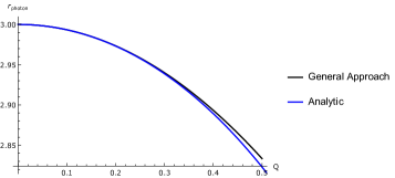
Note that analytic result of photon sphere of Reissner-Nordstrom black hole is
| (19) |
In the Fig. 1, it is seen how change of affect the photon sphere. It is evident that for small values of , the two approaches align closely.
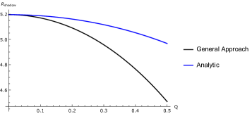
Now, we estimate how the radius of a shadow changes. The shadow radius for the Reissner-Nordstrom black hole is calculated using the general approach as:
| (20) |
Note that analytic result of shadow radius for the Reissner-Nordstrom black hole is
| (21) |
where
In the Fig. 2, it is seen how change of affect the shadow radius of Reissner-Nordstrom black hole using two different method. It is observed that for small values of , the two approaches are in agreement.
II.2 Example: Bardeen Black Hole
Bardeen introduced an exact black hole solution in 1968 Bardeen (1968); Vagnozzi et al. (2023) that does not exhibit singularities at its origin, meaning that the curvature scalar does not tend to infinity. The line element describing the Bardeen regular black hole can be expressed as follows:
| (22) |
Here, represents the mass, and denotes the monopole charge of a self-gravitating magnetic field sourced by non-linear electrodynamics.
The function can be approximated asymptotically as
| (23) |
Using the Eq.2, we can obtain the coefficient for Bardeen black hole as
| (24) |
In order to estimate the influence on the radius of a photon sphere, we assume the radius of a photon sphere
| (25) |
In the Fig. it is seen how change of affect the photon sphere.
Now, we estimate how the radius of a shadow changes. The shadow radius for the Bardeen black hole is calculated using the general approach as:
| (26) |
The shadow radius of the Bardeen black hole decreases as the monopole charge increases.
II.3 Example: Magnetically charged Einstein-Euler-Heisenberg Black Hole
Another example is the magnetically charged black hole solutions derived from the Einstein-Euler-Heisenberg nonlinear electrodynamics, which represents a low-energy limit of Born-Infeld electrodynamics. The metric function for magnetically charged black hole solutions within this theory is given by Allahyari et al. (2020):
| (27) |
where signifies the black hole’s magnetic charge, a defining characteristic, while represents the coupling parameter in the Einstein-Euler-Heisenberg nonlinear electrodynamics (NLED), as outlined in Equation (27). Notably, for , magnetic charges exceeding are allowable.
Utilizing Equation (2), we can derive the coefficient for magnetically charged black holes as:
| (28) | |||
| (29) |
In order to estimate the influence on the radius of a photon sphere, we assume the radius of a photon sphere
| (30) |
Now, we estimate how the radius of a shadow changes. The shadow radius for magnetically charged black hole is calculated using the general approach as:
| (31) |
The photon sphere and shadow radius of the magnetically charged black hole decreases as the magnetic charge increases.
III ESTIMATION HOW RADIUS OF A PHOTON SPHERE CHANGES WITH MASS
In this section, we find a method to estimate how radius of a photon sphere changes with mass. For this purpose we consider general static spherically symmetric spacetime in Eddington-Finkelstein coordinates
| (32) |
This spacetime is supported with anisotropic energy-momentum tensor of the form
| (33) |
The radial component of the four-vector tangent to null geodesic is given by
| (34) |
Where is an effective potential and and are energy and angular momentum respectively. To find unstable photon orbit, one needs to satisfy two conditions (5). The second condition gives us a equation
| (35) |
Now, we will find out how a radius of photon sphere changes if we consider small change of mass of a black hole. For this purpose, we introduce small dimensionless parameter and the mass of black hole becomes . Where corresponds to accretion and to radiation processes respectively. We write the effective potential in the form
| (36) |
For simplicity, we introduce two new functions
| (37) |
Then the second condition (5) gives
| (38) |
Now we assume that the radius of a photon sphere is given by
| (39) |
where is the radius of a photon sphere before accretion or radiation processes. Substituting (39) into (38) and expanding it with respect to alpha we find
| (40) |
Substituting (III) into (40) and evaluating it on the photon sphere, we find
| (41) |
The dominant energy condition demands . From (III), we can write which gives us the dominator of (41) as . From (35), we know that . Thus we have in the denominator of (41) .
In the paper Hod (2020), it was proved that the radius of a photon sphere should be at least , where is the event horizon location. If we substitute it and use the fact that then we find that denominator of (41) less than 1. This fact allows us to state that is always positive.
Theorem (Photon Sphere and Mass):
This implies a direct relationship between the mass and the radius of the photon sphere: as the mass increases, the radius of the photon sphere also increases; conversely, if the mass decreases, so does the radius of the photon sphere .
We can show in the same manner that even we consider the equation of state then this condition is held for an arbitrary .
The mass function depends upon several parameters which describe a black hole.
For example in Reissner-Nordstrom case it depends on both constant mass and electric charge . It may happen, that by increases the mass of black hole and electric charge the radius of photon sphere can decrease. As an example let’s consider the Reissner-Nordstrom spacetime in which mass function is given by
| (42) |
And we consider small positive change in mass and electrical charge by and , where and are small positive constants. By substituting these changes into the mass function (42) and expanding it with respect to and , we arrive at
| (43) |
By choosing parameters and we can make two last terms be negative. It means that we increases mass parameter but decreases the mass function which means that the radius of a photon sphere and shadow decrease.
Now, we shall prove that it is possible only when the weak energy condition is violated. For this purpose, we should understand the nature of parameters and . We consider the accretion or radiating processes. It means that the spacetime should be dynamical one. We write it in the form
| (44) |
Where is the mass function of both time and radial coordinate and depending on ingoing or outgoing flux respectively. The mass function change is described by component of energy-momentum tensor, which reads
| (45) |
In order to satisfy the weak energy condition this flux must be positive which means for accretion and negative for radiation . However, the mass function depends on parameters and which should vary in time, i.e. they should be the functions of time. We consider the accretion process, i.e. . It means
| (46) |
Comparing this expression with , we find
| (47) |
If the mass function decreases it means that decreases which violate weak energy condition.
We prove it only for two parameters but this can be extended for an arbitrary amount of parameters.
We can state it as a theorem.
Theorem:
If the mass of a black hole increases while the weak energy condition holds, the size of the black hole’s shadow also increases.
III.1 Example: Hairy Schwarzschild Black Hole
Our first example is the hairy Schwarzschild black hole, obtained through gravitational decoupling as described in the paper by Ovalle et al. Ovalle et al. (2021). It has the lapse function and the mass function has the following form
| (48) |
and
| (49) |
Here, is the mass of a black hole, is coupling constant and is related to a primary hair. We consider changes in mass and primary hair as
| (50) |
We can write the mass function up to order , as
| (51) |
and
| (52) |
As one can see, under some conditions, the new mass function might be less than , i.e. the radius of a photon sphere decreases despite the mass of a black hole grows. However, it might happen only if .
III.2 Example: Kiselev Black Hole
Kiselev black hole Kiselev (2003) is explicit example that the radius of a photon sphere might decrease while the mass of a black hole grows. The Kiselev solution has the lapse and mass functions of the form
| (53) |
and
| (54) |
Here is a black hole mass, is a cosmological parameter and is a parameter of equation of state. We consider only positive values of . In this case, the cosmological parameter should be always negative. We consider the positive changes of mass and cosmological parameters
| (55) |
In this case as
| (56) |
and one can write it
| (57) |
With negative one can always find such and that .
III.3 Example: Magnetically charged Einstein-Euler-Heisenberg Black Hole
Another example is the magnetically charged black hole solutions within this theory, as described in Allahyari et al. (2020)
| (58) |
where denotes the magnetic charge of the black hole, representing a distinct attribute, while signifies the coupling parameter in the Einstein-Euler-Heisenberg nonlinear electrodynamics (NLED), as detailed in Eq. (58). It’s noteworthy that for , magnetic charges exceeding are admissible.
The metric function for magnetically charged black hole solutions can also be expressed in the following form:
| (59) |
where the function , in this case, is given by:
| (60) |
On the other hand we can also estimate how radius of a photon sphere changes with mass
Here is a black hole mass. and is the magnetic charge which is always positive. We consider the positive changes of mass and charge parameters
| (61) |
In this case as
| (62) | |||
which can be written as
| (63) |
With negative one can always find such and that .
III.4 Example: Black holes in MOdified Gravity (scalar-tensor-vector gravity)
Last example is the black holes in Modified Gravity (MOG black hole) proposed by Moffat in Ref. Moffat (2006), commonly known as scalar-tensor-vector gravity. In this scenario, the metric function describing the resulting black hole solution is given by Moffat (2015).
| (64) |
where the function , in this case, is given by:
| (65) |
Here, is a parameter governing the strength of the effective gravitational coupling , representing a universal hair.
Here is a black hole mass. and is a constant. We consider the positive changes of mass and charge parameters
| (66) |
In this case as
| (67) |
then we rewrite it
| (68) |
With negative one can always find such and that .
IV CONCLUSIONS
A shadow is a critical aspect of a black hole, providing valuable insights into its structure. Modern imaging techniques have enabled us to observe these shadows, prompting a deeper investigation into their characteristics, particularly regarding the influence of various black hole properties like accretion, radiation, and other parameters. Understanding the shadow is pivotal for validating or refuting black hole models. Furthermore, shadows are not exclusive to black holes; other compact objects like wormholes and naked singularities can also cast shadows, offering a means to probe these enigmatic entities Heydarzade and Vertogradov (2023); Shaikh et al. (2019). Shadows also serve as a tool to test the nature of the objects obscured behind them. However, due to the often complex spacetime structures, analytical calculations of photon spheres or shadows are frequently unfeasible, necessitating the use of numerical methods to study their properties.
In this study, we present a novel method for determining the radius of a photon sphere and shadow in any asymptotically flat spherically symmetric spacetime. Our method facilitates a straightforward comparison of photon sphere and shadow radii with those of a Schwarzschild black hole, providing valuable insights into the gravitational effects of various spacetime geometries. We validate our approach by applying it to several well-known examples, demonstrating its efficacy.
Moreover, we address a significant question regarding the shadow of a dynamical black hole. In scenarios involving accretion and radiation processes, the mass of the black hole and the surrounding spacetime geometry evolve dynamically. However, the absence of a timelike Killing vector in dynamical spacetimes poses challenges in reducing the second-order equations of motion to first-order ones. Consequently, numerical methods or the identification of additional symmetries become necessary. In this paper, we take initial steps towards analytically understanding shadows and photon spheres in dynamical spacetimes, focusing specifically on the accretion process.
We show that variations in the mass function of the black hole correlate with changes in the radius of the photon sphere. However, it is crucial to distinguish between the mass function and the actual mass of the black hole, as the former depends on various parameters such as radius and mass. We illustrate this distinction with an example involving the accretion of charged particles, where despite an increase in mass, the radius of the photon sphere decreases due to a higher rate of electrical charge accumulation relative to mass. We rigorously prove, as a theorem, that such scenarios occur only when the weak energy condition is violated. This theorem lays the groundwork for the future development of analytical methods for calculating shadows cast by dynamical black holes, promising advancements in our understanding of these complex phenomena.
Looking towards the future, our work lays the groundwork for further advancements in the field. The next-generation Event Horizon Telescope (ngEHT) promises even more precise tests of gravity near black holes. By continuously leveraging advancements in observational technology, we can refine our understanding of black holes, ultimately leading to a deeper grasp of the fundamental forces governing the universe.
Acknowledgements.
V. Vertogradov thanks the Basis Foundation (grant number 23-1-3-33-1) for the financial support. A. Ö. would like to acknowledge the contribution of the COST Action CA21106 - COSMIC WISPers in the Dark Universe: Theory, astrophysics and experiments (CosmicWISPers) and the COST Action CA22113 - Fundamental challenges in theoretical physics (THEORY-CHALLENGES). We also thank TUBITAK and SCOAP3 for their support.References
- Bardeen (1968) J Bardeen, “Non-singular general-relativistic gravitational collapse, in proceedings of the international conference gr5,” Tbilisi, USSR 174 (1968).
- Luminet (1979) J. P. Luminet, “Image of a spherical black hole with thin accretion disk,” Astron. Astrophys. 75, 228–235 (1979).
- Falcke et al. (2000) Heino Falcke, Fulvio Melia, and Eric Agol, “Viewing the shadow of the black hole at the galactic center,” Astrophys. J. Lett. 528, L13 (2000), arXiv:astro-ph/9912263 .
- Akiyama et al. (2019) Kazunori Akiyama et al. (Event Horizon Telescope), “First M87 Event Horizon Telescope Results. I. The Shadow of the Supermassive Black Hole,” Astrophys. J. Lett. 875, L1 (2019), arXiv:1906.11238 [astro-ph.GA] .
- Akiyama et al. (2022) Kazunori Akiyama et al. (Event Horizon Telescope), “First Sagittarius A* Event Horizon Telescope Results. I. The Shadow of the Supermassive Black Hole in the Center of the Milky Way,” Astrophys. J. Lett. 930, L12 (2022), arXiv:2311.08680 [astro-ph.HE] .
- Bronzwaer and Falcke (2021) Thomas Bronzwaer and Heino Falcke, “The Nature of Black Hole Shadows,” Astrophys. J. 920, 155 (2021), arXiv:2108.03966 [astro-ph.HE] .
- Vagnozzi et al. (2023) Sunny Vagnozzi et al., “Horizon-scale tests of gravity theories and fundamental physics from the Event Horizon Telescope image of Sagittarius A,” Class. Quant. Grav. 40, 165007 (2023), arXiv:2205.07787 [gr-qc] .
- Vertogradov and Övgün (2024) Vitalii Vertogradov and Ali Övgün, “Analyzing the Influence of Geometrical Deformation on Photon Sphere and Shadow Radius: A New Analytical Approach – Part I: Spherically Symmetric Spacetimes,” (2024), arXiv:2404.04046 [gr-qc] .
- Perlick et al. (2015) Volker Perlick, Oleg Yu. Tsupko, and Gennady S. Bisnovatyi-Kogan, “Influence of a plasma on the shadow of a spherically symmetric black hole,” Phys. Rev. D 92, 104031 (2015), arXiv:1507.04217 [gr-qc] .
- Virbhadra (2024) K. S. Virbhadra, “Images Distortion Hypothesis,” (2024), arXiv:2402.17190 [gr-qc] .
- Adler and Virbhadra (2022) Stephen L. Adler and K. S. Virbhadra, “Cosmological constant corrections to the photon sphere and black hole shadow radii,” Gen. Rel. Grav. 54, 93 (2022), arXiv:2205.04628 [gr-qc] .
- Virbhadra (2022) K. S. Virbhadra, “Distortions of images of Schwarzschild lensing,” Phys. Rev. D 106, 064038 (2022), arXiv:2204.01879 [gr-qc] .
- Virbhadra and Keeton (2008) K. S. Virbhadra and C. R. Keeton, “Time delay and magnification centroid due to gravitational lensing by black holes and naked singularities,” Phys. Rev. D 77, 124014 (2008), arXiv:0710.2333 [gr-qc] .
- Virbhadra and Ellis (2000) K. S. Virbhadra and George F. R. Ellis, “Schwarzschild black hole lensing,” Phys. Rev. D 62, 084003 (2000), arXiv:astro-ph/9904193 .
- Virbhadra et al. (1998) K. S. Virbhadra, D. Narasimha, and S. M. Chitre, “Role of the scalar field in gravitational lensing,” Astron. Astrophys. 337, 1–8 (1998), arXiv:astro-ph/9801174 .
- Yang et al. (2024) Yi Yang, Dong Liu, Ali Övgün, Gaetano Lambiase, and Zheng-Wen Long, “Black hole surrounded by the pseudo-isothermal dark matter halo,” Eur. Phys. J. C 84, 63 (2024), arXiv:2308.05544 [gr-qc] .
- Zakharov (2022) Alexander F. Zakharov, “Constraints on a Tidal Charge of the Supermassive Black Hole in M87* with the EHT Observations in April 2017,” Universe 8, 141 (2022), arXiv:2108.01533 [gr-qc] .
- Zakharov (2023) Alexander F. Zakharov, “Constraints on black hole charges in M87* and Sgr A* with the EHT observations,” (2023) arXiv:2305.15446 [gr-qc] .
- Alloqulov et al. (2024) Mirzabek Alloqulov, Farruh Atamurotov, Ahmadjon Abdujabbarov, Bobomurat Ahmedov, and Vokhid Khamidov, “Shadow and weak gravitational lensing for Ellis-Bronnikov wormhole,” Chin. Phys. C 48, 025104 (2024).
- Abdujabbarov et al. (2016) Ahmadjon Abdujabbarov, Muhammed Amir, Bobomurat Ahmedov, and Sushant G. Ghosh, “Shadow of rotating regular black holes,” Phys. Rev. D 93, 104004 (2016), arXiv:1604.03809 [gr-qc] .
- Atamurotov et al. (2013) Farruh Atamurotov, Ahmadjon Abdujabbarov, and Bobomurat Ahmedov, “Shadow of rotating non-Kerr black hole,” Phys. Rev. D 88, 064004 (2013).
- Abdujabbarov et al. (2015) A. A. Abdujabbarov, L. Rezzolla, and B. J. Ahmedov, “A coordinate-independent characterization of a black hole shadow,” Mon. Not. Roy. Astron. Soc. 454, 2423–2435 (2015), arXiv:1503.09054 [gr-qc] .
- Abdikamalov et al. (2019) Askar B. Abdikamalov, Ahmadjon A. Abdujabbarov, Dimitry Ayzenberg, Daniele Malafarina, Cosimo Bambi, and Bobomurat Ahmedov, “Black hole mimicker hiding in the shadow: Optical properties of the metric,” Phys. Rev. D 100, 024014 (2019), arXiv:1904.06207 [gr-qc] .
- Vagnozzi et al. (2020) Sunny Vagnozzi, Cosimo Bambi, and Luca Visinelli, “Concerns regarding the use of black hole shadows as standard rulers,” Class. Quant. Grav. 37, 087001 (2020), arXiv:2001.02986 [gr-qc] .
- Claudel et al. (2001) Clarissa-Marie Claudel, K. S. Virbhadra, and G. F. R. Ellis, “The Geometry of photon surfaces,” J. Math. Phys. 42, 818–838 (2001), arXiv:gr-qc/0005050 .
- Hod (2020) Shahar Hod, “Lower bound on the radii of black-hole photonspheres,” Phys. Rev. D 101, 084033 (2020), arXiv:2012.03962 [gr-qc] .
- Hod (2013a) Shahar Hod, “Spherical null geodesics of rotating Kerr black holes,” Phys. Lett. B 718, 1552–1556 (2013a), arXiv:1210.2486 [gr-qc] .
- Hod (2013b) Shahar Hod, “Marginally bound (critical) geodesics of rapidly rotating black holes,” Phys. Rev. D 88, 087502 (2013b), arXiv:1707.05680 [gr-qc] .
- Hod (2023a) Shahar Hod, “Lower bound on the radii of light rings in traceless black-hole spacetimes,” JHEP 12, 178 (2023a), arXiv:2311.17462 [gr-qc] .
- Hod (2023b) Shahar Hod, “Lower bound on the time-to-mass ratio of closed circular motions around spinning and charged naked singularities,” Eur. Phys. J. C 83, 177 (2023b).
- Khoo and Ong (2016) Fech Scen Khoo and Yen Chin Ong, “Lux in obscuro: Photon Orbits of Extremal Black Holes Revisited,” Class. Quant. Grav. 33, 235002 (2016), [Erratum: Class.Quant.Grav. 34, 219501 (2017)], arXiv:1605.05774 [gr-qc] .
- Decanini et al. (2010) Yves Decanini, Antoine Folacci, and Bernard Raffaelli, “Unstable circular null geodesics of static spherically symmetric black holes, Regge poles and quasinormal frequencies,” Phys. Rev. D 81, 104039 (2010), arXiv:1002.0121 [gr-qc] .
- Pantig et al. (2022) Reggie C. Pantig, Leonardo Mastrototaro, Gaetano Lambiase, and Ali Övgün, “Shadow, lensing, quasinormal modes, greybody bounds and neutrino propagation by dyonic ModMax black holes,” Eur. Phys. J. C 82, 1155 (2022), arXiv:2208.06664 [gr-qc] .
- Shoom (2017) Andrey A. Shoom, “Metamorphoses of a photon sphere,” Phys. Rev. D 96, 084056 (2017), arXiv:1708.00019 [gr-qc] .
- Konoplya and Zhidenko (2021) R. A. Konoplya and A. Zhidenko, “Shadows of parametrized axially symmetric black holes allowing for separation of variables,” Phys. Rev. D 103, 104033 (2021), arXiv:2103.03855 [gr-qc] .
- Kuang and Övgün (2022) Xiao-Mei Kuang and Ali Övgün, “Strong gravitational lensing and shadow constraint from M87* of slowly rotating Kerr-like black hole,” Annals Phys. 447, 169147 (2022), arXiv:2205.11003 [gr-qc] .
- Bronnikov et al. (2021) Kirill A. Bronnikov, Roman A. Konoplya, and Thomas D. Pappas, “General parametrization of wormhole spacetimes and its application to shadows and quasinormal modes,” Phys. Rev. D 103, 124062 (2021), arXiv:2102.10679 [gr-qc] .
- Paithankar and Kolekar (2023) Kajol Paithankar and Sanved Kolekar, “Black hole shadow and acceleration bounds for spherically symmetric spacetimes,” Phys. Rev. D 108, 104042 (2023), arXiv:2305.07444 [gr-qc] .
- Konoplya et al. (2016) Roman Konoplya, Luciano Rezzolla, and Alexander Zhidenko, “General parametrization of axisymmetric black holes in metric theories of gravity,” Phys. Rev. D 93, 064015 (2016), arXiv:1602.02378 [gr-qc] .
- Johannsen and Psaltis (2011) Tim Johannsen and Dimitrios Psaltis, “A Metric for Rapidly Spinning Black Holes Suitable for Strong-Field Tests of the No-Hair Theorem,” Phys. Rev. D 83, 124015 (2011), arXiv:1105.3191 [gr-qc] .
- Cardoso et al. (2014) Vitor Cardoso, Paolo Pani, and Joao Rico, “On generic parametrizations of spinning black-hole geometries,” Phys. Rev. D 89, 064007 (2014), arXiv:1401.0528 [gr-qc] .
- Konoplya and Zhidenko (2019) R. A. Konoplya and A. Zhidenko, “Analytical representation for metrics of scalarized Einstein-Maxwell black holes and their shadows,” Phys. Rev. D 100, 044015 (2019), arXiv:1907.05551 [gr-qc] .
- Qiao (2022) Chen-Kai Qiao, “Curvatures, photon spheres, and black hole shadows,” Phys. Rev. D 106, 084060 (2022), arXiv:2208.01771 [gr-qc] .
- Kokkotas et al. (2017) K. Kokkotas, R. A. Konoplya, and A. Zhidenko, “Non-Schwarzschild black-hole metric in four dimensional higher derivative gravity: analytical approximation,” Phys. Rev. D 96, 064007 (2017), arXiv:1705.09875 [gr-qc] .
- Hennigar et al. (2018) Robie A. Hennigar, Mohammad Bagher Jahani Poshteh, and Robert B. Mann, “Shadows, Signals, and Stability in Einsteinian Cubic Gravity,” Phys. Rev. D 97, 064041 (2018), arXiv:1801.03223 [gr-qc] .
- Konoplya et al. (2020) R. A. Konoplya, A. F. Zinhailo, and Z. Stuchlik, “Quasinormal modes and Hawking radiation of black holes in cubic gravity,” Phys. Rev. D 102, 044023 (2020), arXiv:2006.10462 [gr-qc] .
- Aratore et al. (2024) Fabio Aratore, Oleg Yu. Tsupko, and Volker Perlick, “Constraining spherically symmetric metrics by the gap between photon rings,” (2024), arXiv:2402.14733 [gr-qc] .
- Tsupko (2022) Oleg Yu. Tsupko, “Shape of higher-order images of equatorial emission rings around a Schwarzschild black hole: Analytical description with polar curves,” Phys. Rev. D 106, 064033 (2022), arXiv:2208.02084 [gr-qc] .
- Cederbaum and Galloway (2016) Carla Cederbaum and Gregory J. Galloway, “Uniqueness of photon spheres in electro-vacuum spacetimes,” Class. Quant. Grav. 33, 075006 (2016), arXiv:1508.00355 [math.DG] .
- Johannsen (2013) Tim Johannsen, “Photon Rings around Kerr and Kerr-like Black Holes,” Astrophys. J. 777, 170 (2013), arXiv:1501.02814 [astro-ph.HE] .
- Teo (2003) Edward Teo, “Spherical Photon Orbits Around a Kerr Black Hole,” Gen. Rel. Grav. 35, 1909–1926 (2003).
- Okyay and Övgün (2022) Mert Okyay and Ali Övgün, “Nonlinear electrodynamics effects on the black hole shadow, deflection angle, quasinormal modes and greybody factors,” JCAP 01, 009 (2022), arXiv:2108.07766 [gr-qc] .
- Lu and Lyu (2020) H. Lu and Hong-Da Lyu, “Schwarzschild black holes have the largest size,” Phys. Rev. D 101, 044059 (2020), arXiv:1911.02019 [gr-qc] .
- Younsi et al. (2016) Ziri Younsi, Alexander Zhidenko, Luciano Rezzolla, Roman Konoplya, and Yosuke Mizuno, “New method for shadow calculations: Application to parametrized axisymmetric black holes,” Phys. Rev. D 94, 084025 (2016), arXiv:1607.05767 [gr-qc] .
- Tsupko and Bisnovatyi-Kogan (2020) Oleg Yu. Tsupko and Gennady S. Bisnovatyi-Kogan, “First analytical calculation of black hole shadow in McVittie metric,” Int. J. Mod. Phys. D 29, 2050062 (2020), arXiv:1912.07495 [gr-qc] .
- Tsukamoto et al. (2014) Naoki Tsukamoto, Zilong Li, and Cosimo Bambi, “Constraining the spin and the deformation parameters from the black hole shadow,” JCAP 06, 043 (2014), arXiv:1403.0371 [gr-qc] .
- Ghosh et al. (2023) Rajes Ghosh, Selim Sk, and Sudipta Sarkar, “Hairy black holes: Nonexistence of short hairs and a bound on the light ring size,” Phys. Rev. D 108, L041501 (2023), arXiv:2306.14193 [gr-qc] .
- Övgün et al. (2024) Ali Övgün, Reggie C. Pantig, and Ángel Rincón, “Shadow and greybody bounding of a regular scale-dependent black hole solution,” Annals Phys. 463, 169625 (2024), arXiv:2402.14190 [gr-qc] .
- Adair et al. (2020) Connor Adair, Pablo Bueno, Pablo A. Cano, Robie A. Hennigar, and Robert B. Mann, “Slowly rotating black holes in Einsteinian cubic gravity,” Phys. Rev. D 102, 084001 (2020), arXiv:2004.09598 [gr-qc] .
- Tsukamoto (2018) Naoki Tsukamoto, “Black hole shadow in an asymptotically-flat, stationary, and axisymmetric spacetime: The Kerr-Newman and rotating regular black holes,” Phys. Rev. D 97, 064021 (2018), arXiv:1708.07427 [gr-qc] .
- Gómez and Valageas (2024) Gabriel Gómez and Patrick Valageas, “Constraining Self-interacting Scalar Field Dark Matter From the Black Hole Shadow of the Event Horizon Telescope,” (2024), arXiv:2403.08988 [astro-ph.CO] .
- Shaikh et al. (2019) Rajibul Shaikh, Prashant Kocherlakota, Ramesh Narayan, and Pankaj S. Joshi, “Shadows of spherically symmetric black holes and naked singularities,” Mon. Not. Roy. Astron. Soc. 482, 52–64 (2019), arXiv:1802.08060 [astro-ph.HE] .
- Lambiase et al. (2023) Gaetano Lambiase, Leonardo Mastrototaro, Reggie C. Pantig, and Ali Ovgun, “Probing Schwarzschild-like black holes in metric-affine bumblebee gravity with accretion disk, deflection angle, greybody bounds, and neutrino propagation,” JCAP 12, 026 (2023), arXiv:2309.13594 [gr-qc] .
- Karshiboev et al. (2024) Khurshid Karshiboev, Farruh Atamurotov, Ahmadjon Abdujabbarov, Ali Övgün, and Anvar Reyimberganov, “Exploring the shadow of a rotating charged ModMax black hole,” Commun. Theor. Phys. 76, 025401 (2024).
- Rayimbaev et al. (2023) Javlon Rayimbaev, Reggie C. Pantig, Ali Övgün, Ahmadjon Abdujabbarov, and Durmuş Demir, “Quasiperiodic oscillations, weak field lensing and shadow cast around black holes in Symmergent gravity,” Annals Phys. 454, 169335 (2023), arXiv:2206.06599 [gr-qc] .
- Mustafa et al. (2022) Ghulam Mustafa, Farruh Atamurotov, Ibrar Hussain, Sanjar Shaymatov, and Ali Övgün, “Shadows and gravitational weak lensing by the Schwarzschild black hole in the string cloud background with quintessential field*,” Chin. Phys. C 46, 125107 (2022), arXiv:2207.07608 [gr-qc] .
- Pantig et al. (2023) Reggie C. Pantig, Ali Övgün, and Durmuş Demir, “Testing symmergent gravity through the shadow image and weak field photon deflection by a rotating black hole using the M87∗ and Sgr. results,” Eur. Phys. J. C 83, 250 (2023), arXiv:2208.02969 [gr-qc] .
- Pantig and Övgün (2023) Reggie C. Pantig and Ali Övgün, “Black Hole in Quantum Wave Dark Matter,” Fortsch. Phys. 71, 2200164 (2023), arXiv:2210.00523 [gr-qc] .
- Kumaran and Övgün (2023) Yashmitha Kumaran and Ali Övgün, “Shadow and deflection angle of asymptotic, magnetically-charged, non-singular black hole,” Eur. Phys. J. C 83, 812 (2023), arXiv:2306.04705 [gr-qc] .
- Çimdiker et al. (2023) İlim İrfan Çimdiker, Ali Övgün, and Durmuş Demir, “Thin accretion disk images of the black hole in symmergent gravity,” Class. Quant. Grav. 40, 184001 (2023), arXiv:2308.03947 [gr-qc] .
- Puliçe et al. (2023) Beyhan Puliçe, Reggie C. Pantig, Ali Övgün, and Durmuş Demir, “Constraints on charged symmergent black hole from shadow and lensing,” Class. Quant. Grav. 40, 195003 (2023), arXiv:2308.08415 [gr-qc] .
- Övgün et al. (2018) Ali Övgün, İzzet Sakallı, and Joel Saavedra, “Shadow cast and Deflection angle of Kerr-Newman-Kasuya spacetime,” JCAP 10, 041 (2018), arXiv:1807.00388 [gr-qc] .
- Heydarzade and Vertogradov (2023) Yaghoub Heydarzade and Vitalii Vertogradov, “Dynamical Photon Spheres in Charged Black Holes and Naked Singularities,” (2023), arXiv:2311.08930 [gr-qc] .
- Allahyari et al. (2020) Alireza Allahyari, Mohsen Khodadi, Sunny Vagnozzi, and David F. Mota, “Magnetically charged black holes from non-linear electrodynamics and the Event Horizon Telescope,” JCAP 02, 003 (2020), arXiv:1912.08231 [gr-qc] .
- Pedrotti and Vagnozzi (2024) Davide Pedrotti and Sunny Vagnozzi, “See the lightning, hear the thunder: quasinormal modes-shadow correspondence for rotating regular black holes,” (2024), arXiv:2404.07589 [gr-qc] .
- Tiede et al. (2022) Paul Tiede, Michael D. Johnson, Dominic W. Pesce, Daniel C. M. Palumbo, Dominic O. Chang, and Peter Galison, “Measuring Photon Rings with the ngEHT,” Galaxies 10, 111 (2022), arXiv:2210.13498 [astro-ph.HE] .
- Ayzenberg et al. (2023) D. Ayzenberg et al., “Fundamental Physics Opportunities with the Next-Generation Event Horizon Telescope,” (2023), arXiv:2312.02130 [astro-ph.HE] .
- Perlick and Tsupko (2022) Volker Perlick and Oleg Yu. Tsupko, “Calculating black hole shadows: Review of analytical studies,” Phys. Rept. 947, 1–39 (2022), arXiv:2105.07101 [gr-qc] .
- Ishihara et al. (2016) Asahi Ishihara, Yusuke Suzuki, Toshiaki Ono, Takao Kitamura, and Hideki Asada, “Gravitational bending angle of light for finite distance and the Gauss-Bonnet theorem,” Phys. Rev. D 94, 084015 (2016), arXiv:1604.08308 [gr-qc] .
- Kudo and Asada (2022) Ryuya Kudo and Hideki Asada, “Nondivergent deflection of light around a photon sphere of a compact object,” Phys. Rev. D 105, 084014 (2022), arXiv:2201.01946 [gr-qc] .
- Tan (2023) Hai Siong Tan, “Shadows of Kerr–Vaidya-like black holes,” Class. Quant. Grav. 40, 195010 (2023), arXiv:2301.04967 [gr-qc] .
- Koga et al. (2022) Yasutaka Koga, Nobuyuki Asaka, Masashi Kimura, and Kazumasa Okabayashi, “Dynamical photon sphere and time evolving shadow around black holes with temporal accretion,” Phys. Rev. D 105, 104040 (2022), arXiv:2202.00201 [gr-qc] .
- Solanki and Perlick (2022) Jay Solanki and Volker Perlick, “Photon sphere and shadow of a time-dependent black hole described by a Vaidya metric,” Phys. Rev. D 105, 064056 (2022), arXiv:2201.03274 [gr-qc] .
- Mishra et al. (2019) Akash K. Mishra, Sumanta Chakraborty, and Sudipta Sarkar, “Understanding photon sphere and black hole shadow in dynamically evolving spacetimes,” Phys. Rev. D 99, 104080 (2019), arXiv:1903.06376 [gr-qc] .
- Rodríguez et al. (2024) Benito Rodríguez, Javier Chagoya, and C. Ortiz, “Shadows of black holes in dynamical Chern-Simons modified gravity,” (2024), arXiv:2403.13062 [gr-qc] .
- Bambi (2017) Cosimo Bambi, “Testing black hole candidates with electromagnetic radiation,” Rev. Mod. Phys. 89, 025001 (2017), arXiv:1509.03884 [gr-qc] .
- Shcherbakov et al. (2012) Roman V. Shcherbakov, Robert F. Penna, and Jonathan C. McKinney, “Sagittarius A* Accretion Flow and Black Hole Parameters from General Relativistic Dynamical and Polarized Radiative Modeling,” Astrophys. J. 755, 133 (2012), arXiv:1007.4832 [astro-ph.HE] .
- Psaltis (2019) Dimitrios Psaltis, “Testing General Relativity with the Event Horizon Telescope,” Gen. Rel. Grav. 51, 137 (2019), arXiv:1806.09740 [astro-ph.HE] .
- Cunha et al. (2018) Pedro V. P. Cunha, Carlos A. R. Herdeiro, and Maria J. Rodriguez, “Does the black hole shadow probe the event horizon geometry?” Phys. Rev. D 97, 084020 (2018), arXiv:1802.02675 [gr-qc] .
- Ayzenberg and Yunes (2018) Dimitry Ayzenberg and Nicolas Yunes, “Black Hole Shadow as a Test of General Relativity: Quadratic Gravity,” Class. Quant. Grav. 35, 235002 (2018), arXiv:1807.08422 [gr-qc] .
- Wang et al. (2018) Mingzhi Wang, Songbai Chen, and Jiliang Jing, “Shadows of Bonnor black dihole by chaotic lensing,” Phys. Rev. D 97, 064029 (2018), arXiv:1710.07172 [gr-qc] .
- Cunha and Herdeiro (2018) Pedro V. P. Cunha and Carlos A. R. Herdeiro, “Shadows and strong gravitational lensing: a brief review,” Gen. Rel. Grav. 50, 42 (2018), arXiv:1801.00860 [gr-qc] .
- Cunha et al. (2015) Pedro V. P. Cunha, Carlos A. R. Herdeiro, Eugen Radu, and Helgi F. Runarsson, “Shadows of Kerr black holes with scalar hair,” Phys. Rev. Lett. 115, 211102 (2015), arXiv:1509.00021 [gr-qc] .
- Cunha et al. (2017a) Pedro V. P. Cunha, Carlos A. R. Herdeiro, Burkhard Kleihaus, Jutta Kunz, and Eugen Radu, “Shadows of Einstein–dilaton–Gauss–Bonnet black holes,” Phys. Lett. B 768, 373–379 (2017a), arXiv:1701.00079 [gr-qc] .
- Cunha et al. (2017b) Pedro V. P. Cunha, Carlos A. R. Herdeiro, and Eugen Radu, “Fundamental photon orbits: black hole shadows and spacetime instabilities,” Phys. Rev. D 96, 024039 (2017b), arXiv:1705.05461 [gr-qc] .
- Lima et al. (2021) Haroldo C. D. Lima, Junior., Luís C. B. Crispino, Pedro V. P. Cunha, and Carlos A. R. Herdeiro, “Can different black holes cast the same shadow?” Phys. Rev. D 103, 084040 (2021), arXiv:2102.07034 [gr-qc] .
- Cunha et al. (2017c) Pedro V. P. Cunha, Emanuele Berti, and Carlos A. R. Herdeiro, “Light-Ring Stability for Ultracompact Objects,” Phys. Rev. Lett. 119, 251102 (2017c), arXiv:1708.04211 [gr-qc] .
- Churilova (2019) M. S. Churilova, “Analytical quasinormal modes of spherically symmetric black holes in the eikonal regime,” Eur. Phys. J. C 79, 629 (2019), arXiv:1905.04536 [gr-qc] .
- Ovalle et al. (2021) J. Ovalle, R. Casadio, E. Contreras, and A. Sotomayor, “Hairy black holes by gravitational decoupling,” Phys. Dark Univ. 31, 100744 (2021), arXiv:2006.06735 [gr-qc] .
- Kiselev (2003) V. V. Kiselev, “Quintessence and black holes,” Class. Quant. Grav. 20, 1187–1198 (2003), arXiv:gr-qc/0210040 .
- Moffat (2006) J. W. Moffat, “Scalar-tensor-vector gravity theory,” JCAP 03, 004 (2006), arXiv:gr-qc/0506021 .
- Moffat (2015) J. W. Moffat, “Black Holes in Modified Gravity (MOG),” Eur. Phys. J. C 75, 175 (2015), arXiv:1412.5424 [gr-qc] .