Towards Classical Software Verification using Quantum Computers

Abstract

We explore the possibility of accelerating the formal verification of classical programs with a quantum computer.

A common source of security flaws stems from the existence of common programming errors like use after free, null-pointer dereference, or division by zero. To aid in the discovery of such errors, we try to verify that no such flaws exist.

In our approach, for some code snippet and undesired behaviour, a SAT instance is generated, which is satisfiable precisely if the behavior is present in the code. It is in turn converted to an optimization problem, that is solved on a quantum computer. This approach holds the potential of an asymptotically polynomial speedup.

Minimal examples of common errors, like out-of-bounds and overflows, but also synthetic instances with special properties, specific number of solutions, or structure, are tested with different solvers and tried on a quantum device.

We use the near-standard Quantum Approximation Optimisation Algorithm, an application of the Grover algorithm, and the Quantum Singular Value Transformation to find the optimal solution, and with it a satisfying assignment.

I Introduction

Software testing represents a critical phase in the software development lifecycle, ensuring the reliability, security, and proper functioning of software systems. Proper software verification and validation also provide a lot of potential for cost savings, especially when applied early in the software development process. By identifying and correcting flaws before they can propagate through later stages of development or, worse, into deployed systems, organizations can avoid the exorbitant costs associated with post-deployment fixes, not to mention the potential for harm to users and damage to the organization’s reputation.

Especially for systems with a high cost of failure, like the control software for critical infrastructure or software for medical devices, the importance of rigorous testing cannot be overstated. One tragic example highlighting the potential consequences of inadequate software testing is the Therac-25 incident, where flaws in the software controlling a radiation therapy machine led to patient fatalities and injuries [1]. This incident underscores not just the need for thorough software testing but also for methods that can guarantee correctness and safety. Among these methods, formal verification emerges as a powerful approach, offering mathematical proofs of correctness that traditional testing methods cannot.

Formal verification methods apply mathematical models to verify the correctness of software with respect to a formal specification of its intended behavior. This includes the inputs it will receive, the outputs it should (or must never) produce, and the rules governing its behavior, where the first and last point can usually be derived from the software’s source code while specifying the outputs relates to the software’s functional (or security) requirements. A typical specification, for example for a banking transaction system, could be that the balance of an account should never become negative after a transaction. Another example of a more low-level security-relevant specification is guaranteeing that no memory outside the bounds of an array is accessed. There is a variety of techniques and tools available that build a suitable abstract model from the source code and specification of properties that need to be verified. Symbolic execution engines, e.g. [2], often result in a Satisfiability Modulo Theory (SMT) problems [3], other approaches are based on reachability in the code’s so-called Control Flow Graph (CFG) [4], which allows a more abstract view of programs.

Being able to formally proof properties of code is a huge advantage, however, the application of formal verification and model checking is not without its challenges. Rice’s theorem [5], a fundamental result in computer science, asserts that if a property does not hold for all or no program, no algorithm exist, that can correctly decide for all possible programs, if the property holds or not. This theorem sets a theoretical limit on the capabilities of formal verification, implying that we must severely restrict ourselves concerning the possible properties we wish to certify. A well-known corollary of this is the famous halting problem [6] which is undecidable.

Moreover, the computational demands of formal verification are significant. Even if a verification problem is decidable, it is very often also NP-hard. Intuitively, this can also be understood considering that every decision node in the CFG potentially doubles the amount of paths that need to be checked.

Here, quantum computing might help to solve these types of problems more efficiently in the future. In the following paper, we evaluate different possible approaches and quantum algorithms towards this goal. To that end, we introduce an end-to-end pipeline all the way from code snippets to the solution of the satisfiability problem corresponding to the desired verification task.

Our approach starts with a file of C-code and takes the following steps, also depicted in Figure 1 on page 1.

1. The checked properties are specified as flags for the converter.

2. A SAT formula, that is precisely satisfiable if a problematic input exists, is generated.

3. The formula is manipulated classically, to optimize its number of variables, depth, or logical operations.

4. An optimization problem is generated from the resulting formula.

5. The optimal solution is found with the help of a quantum device.

Different solvers are used and more are planned for future work.

Figure 1: Overview of the full process

In summary, our contributions are as follows:

• A technique to transform a SAT instance to a QUBO with a guaranteed gap between possible values and a minimum depending on the satisfiability of the instance.

• An end-to-end implementation of the full verification task from a C-file to the guarantee of a flaw or its likely absence.

• The Initial assessment of three different approaches to solving the resulting optimization problem with a quantum algorithm.

I-A Structure

We start in Section III with some intuition as to how these formulae are constructed and how we generate them. Section IV explores the construction of the optimization problem from the formula. As the last step, we see in Section V, how we solve the optimization problem with the use of a quantum computer. With this, we present our performed experiments and compare how the used solvers perform on specific instances in Section VI.

II Related Work

The exploration of quantum computing in software verification is a novel endeavor that seeks to harness quantum mechanics to improve the efficiency of verifying classical software systems. To date, the majority of related research has focused on problems such as quantum circuit verification or software verification with classical computers. However, there has been a gap in the literature when it comes to applying quantum computing to classical software verification tasks.

To work with large systems, one approach is to divide the whole system into individual components. By handling these components as modules, with special compositional algorithms, it is possible to handle much larger state spaces. For an introduction to compositional methods and a survey of used algorithms see [7].

Even perfect protection from errors is worthless, if it is not applied in practice, may it be for the cost in time and resources or because only a specialised expert could use the techniques. At least one study exists, where the practicality of formal verification results is evaluated, see [8].

A large theoretical field is Model Checking, to some degree a generalization of the satisfiability problem. A common approach for formal verification is to formulate the considered properties logically and checking if a model, here input, exists for the code and negated property. See the book [9] for a quite recent overview of model checking, program verification, static analysis and more.

While not directly related to classical software verification, Quantum Circuit Verification does have many similarities to it. See [10], where a way to model quantum circuits is explored. Such a model can than be handled like the classical case, allowing the properties and behaviors of quantum circuits to be verified.

With all its theoretical works, there is also an abundance of tools for different verification tasks, like formal methods, statics analysis and testing, a survey can be found in [11].

There are different approaches to software verification, that theorists strive to unify. For this goal, multiple frameworks can be defined, where each has different strengths and weaknesses. One such framework, together with a survey of multiple verification tasks, is presented in [12].

The work in this paper represents the first practical attempt to apply quantum computing to accelerate the verification of classical software systems, to the best of our knowledge. By building upon the existing theoretical frameworks and leveraging the unique computational capabilities of quantum machines, this research aims to open a new frontier in software verification.

III Generating a SAT instance

In this section, we turn the question of whether some property holds for our code, into a logical formula.

III-A Introduction to Satisfiability of Different Logics

The Satisfiability Problem (SAT) asks for a given boolean formula if there exists an assignment of its variables that satisfies the formula. They are built from variables that can take the values $\mathrm{TRUE}$ or $\mathrm{FALSE}$, and the operators $\land$ AND, $\lor$ OR, and $\neg$ NOT.

This problem is known to be NP-complete, see [13], which makes it computationally expensive to solve, but also of great interest to be solved.

We can restrict the input to a special form, the Conjunctive Normal Form (CNF). For $n\in\mathbb{N}$ variables $X_{1},\ldots,X_{n}$ and some $1\leq k\leq n$, we call

$$\bigvee_{j=1}^{k}L_{j}$$

a clause, where $L_{j}=X_{J^{\prime}}$ or $L_{j}=\neg X_{j^{\prime}}$ is called a literal of the variable $j^{\prime}$. Here, the $L_{j}$ are restricted to contain pairwise different variables, otherwise the clause can be simplified by $X\lor X=X$ and $X\lor\neg X=\mathrm{TRUE}$. A formula is in CNF, if it is a conjunction of pairwise different clauses over its variables. For $1\leq l\leq 2^{n}$, it is of the form

$$\bigwedge_{i=1}^{l}\bigvee_{j=1}^{k_{i}}L_{ij}$$

where the clauses are never proper sub-clauses of each other.

Every formula can be converted to this form with polynomial overhead, so we can assume the input to already be given in CNF.

While this problem is already hard, it is logically quite restrictive. It is equivalent to asking if the same formula $\varphi(x_{1},\ldots,x_{n})$, where every variable is bound by an existential quantifier $\exists x_{1}\ldots\exists x_{n}\varphi(x_{1},\ldots,x_{n})$, is equivalent to $\mathrm{TRUE}$. Allowing the quantifiers to be universal $\forall$ as well, makes the problem much harder, PSPACE-complete to be precise, as shown in [14].

Even this extension is not enough for our problems. In this very general setting of a general program and some property of interest, even richer logics would be necessary. Not only does the need to express integers and their arithmetic arise, but we also need stronger quantifiers to express unconditional recursive calls. This leads to Symbolic Model Theory (SMT), and higher order logic, like second-order logic. Since these concepts will not be used in this work, but only referenced as a problem, no further introduction is needed and left for future work.

III-B Expressing the Existence of Errors as a Formula

By formally verifying software, we mean proving that some defined property holds for every input to the software. Typical properties of interest are related to run time or general software errors, such as no buffer ever overflowing or a function output always being inside a valid range. Such a property excludes many possibilities for a potential attacker to exploit the system and ensures that the program behaves as expected even for unaccounted inputs.

For many properties of interest, this can be rephrased to a reachability problem of specific bad states, and, equivalently, if one specific state is reachable. This is possible if the property can be checked locally, like an Out of Bounds error with known bounds. By checking if the bound is respected, the program flow can be split into normal and erroneous behavior. For this, the Control Flow Graph (CFG) is often considered. This graph encodes different code regions as vertices and the transitions between them as edges. In this case, a special error state is added, where all the erroneous paths lead.

As a minimal example, see the tiny C-Program with an Out of Bounds error and a possible CFG in Figure 2 on page 2.

⬇ int main(void) { int buf[1]; int i = 1; buf[i] = 0; return 0; } $\Longrightarrow$

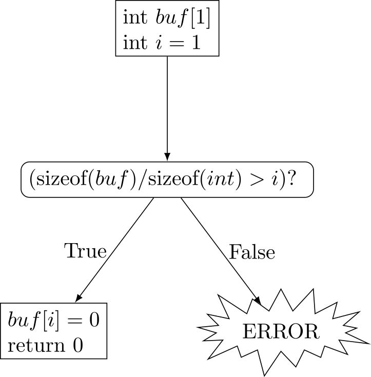
Figure 2: Minimal Out of Bounds error and a possible CFG with a single error state.

The program flow is augmented to lead into one specific error state, in case the check fails. All (and only) the erroneous paths will lead to this new state, so precisely the undesired executions will reach it. This is done for all errors, reducing the question of the existence of errors to the reachability of this one state.

How the logical expression is obtained from the CFG is a problem of its own. Every vertex in the CFG is assigned a formula, that corresponds to the operation its corresponding code performed. So is every edge, except that the formula encodes if the corresponding transition is taken in the code. All these formulae are now combined to get a potentially higher-order formula. This explanation should give some intuition to the procedure, see [15] and [16] for a much more complete explanation.

We point out again that the resulting formula might contain integers and could even be of higher order. To handle these problems, we must generally make restricting assumptions. Integers can be upper- and lower-bound, and higher-order operators can be bound with further assumptions about the possible models. With these assumptions, it is no longer possible to find all solutions, only the ones allowed by these restrictions. This means that our process will only find valid solutions, making it correct, but if no solution is found, one might still exist, so it is no longer complete. This is not surprising, otherwise we could do the impossible and solve the Halting problem by constructing a program that for the input $f,x$ evaluates $f(x)$, followed by a single error state. The error state is reached if and only if $f$ holds for input $x$.

As an example for some reasonable restrictions, we might assume that used integers are formed by $64$ bits and the maximum recursive depth is $2^{512}$. This restricts the function to a finite number of possible states, which might be a huge number of possibilities, but finite, turning the problem solvable.

For this work, the conversion is performed by existing tools, concretely CBMC [17], where the output is always a SAT instance. CBMC can be configured to what errors it checks for and performs the needed modifications automatically. Other tools, such as Seahorn [18], were considered and some are planned to be used in future work.

The resulting SAT formula is in CNF form and parsed with PySMT [19]. This allows Z3 [20], a symbolic logic as well as SAT solver, to be called directly, so all its simplification and conversion abilities can easily be used. Simplified formulae should only be smaller, so even if they are too large to fit on a QC before they get simplified, they might after. Conversions are useful to test different formulations of the same formula. They might result in different optimization problems, where one is easier to solve than the others.

IV Generating the Optimization Problem

The Quadratic Unconstrained Binary Optimization (QUBO) formulation is particularly fitting for quantum computing, because it naturally maps binary variables and objective functions into the language of qubits and quantum gates.

A QUBO is given by

$$\operatorname*{argmin}_{x\in\{0,1\}^{n}}x^{T}Qx+c$$

for $Q\in\mathbb{R}^{n\times n}$ and $c\in\mathbb{R}$. This formulation nicely maps to the Ising model, see [21] for details, that in turn can be easily mapped to some hardware. This close relation to potential hardware made them very popular, for a great overview see [22].

Note that this can be seen as a quadratic polynomial with the variables $x_{1},\ldots x_{n}$, where the linear terms are in the diagonal of $Q$.

A general Quadratic Program (QP) has a few differences. Its variables are not restricted to binary values, but are instead real numbers. The second big difference is, that we are not just interested in any minimum, but only the ones that fulfill additional constraints. They are of the form

$$Ax\geq C$$

for $A\in\mathbb{R}^{k\times n}$ and $C\in\mathbb{R}^{k}$ with $k\in\mathbb{N}$ the number of constraints. Here $\geq$ is meant to hold component-wise.

If we restrict the variables to the integers, we get an Integer Quadratic Program (IQP) and by allowing both real and integer values, we get a Mixed Integer Quadratic Program (MIQP).

IV-A Satisfiability as Optimum in a Quadratic Program

To convert a logical formula into an IQP, we have to map its logical structure to an arithmetic equivalent. This has to be done carefully to keep all valid assignments, but also not introduce new ones. The easiest examples are the negation $\neg x$, which corresponds to subtraction $1-x$, and the disjunction $x\land y$, that easily maps to multiplication $x\cdot y$. In this approach, We can see that we already get problems with a conjunction of three variables $x\land y\land z$. It would result in $x\cdot y\cdot z$, a cubic polynomial. To avoid higher degrees, we have to introduce an additional variable $t$ and carefully design a polynomial to represent $t=x\cdot y$, by also adding $t\cdot z$, we can represent the formula only with quadratic terms.

A direct way to encode a logical expression in a QP is to include it as a constraint. For instance, the formula $\bigwedge_{j}x_{j}$ could be included as $\sum_{j}x_{j}\geq 1$. A negation can be directly included by the substitution $x\mapsto 1-x$, which shows how clauses might be enforced to hold. Since a conjunction can be realized by enforcing all its arguments to hold, we can already represent any formula in CNF as an IQP, by restricting the variables to be binary $0\leq x\leq 1$ as well.

This would work, but to get a QUBO, we must encode the constraints into the objective, the standard way is to do this as penalties. For constraint $\sum_{j=1}^{k}a_{j}x_{j}\geq c$ where $k\in\mathbb{N}$ and $a_{j},c\in\mathbb{R}\;\forall 1\leq j\leq k$, this is done as follows. By introducing a slack variable $s\in\mathbb{N}$, we can reformulate it into an equality.

$$\sum_{j}a_{j}x_{j}\geq c\iff\exists s\geq 0\colon\sum_{j}a_{j}x_{j}=c+s$$

Now, to get the penalty, we square the difference of both sides and multiply it by some weight $M>0$. This leads to

$$M\left(\sum_{j}a_{j}x_{j}-c-s\right)^{2}=0$$

which is added to the objective function.

For $M\to\infty$, only solutions satisfying the constraint can have a finite objective. At the same time, a large $M$ means that all other factors will get relatively close to zero after normalizing. This means even higher precision will be needed to find a proper solution. A large enough $M$ will have to be found for the concrete problem as well, the smallest possible is preferred.

The introduced slack variables have to be dealt with as well. Since they are not binary, but natural numbers, we have to approximate them with weighted sums of binary variables. This will use even more variables and needs an upper limit for the slack variables as well.

IV-B Satisfiability by Unconstrained Optimization Problems

To get around some of these problems, especially the slack variables, we will directly encode the formula in the objective function. We will consider any SAT formula and not just CNF, therefor our construction must be able to handle logical operators, but also the sub-formulae they take as arguments.

To do this, we have to map the logical operators to arithmetic expressions. Since we are searching for satisfying assignments, the arithmetic expressions will be chosen to have their minima at precisely the satisfying assignments. Our goal is to construct a QUBO, so quadratic polynomials will be used in our case.

By constructing the minima of all our polynomials to be at zero, we ensure that the minimum of the sum over them is bounded from below by zero. This minimum can only be reached, if all sub-expressions reach their minimum at the same time. By introducing additional variables that represent the sub-formulae, we construct a polynomial for every operator and take the sum over them. If an assignment reaches a minimum of zero, the assignment is satisfying and all extra variables are assigned to represent their sub-formula by construction. Conversely, a satisfying assignment can be extended with the extra variables to form a minimum of zero for every expression.

We start with the base case of a single variable $x$. The optimization problem also has a corresponding variable $x$. By adding $1-x$ to the objective, the minimum of zero will now be reached for $x=1$ and its value is one for $x=0$. Similar for $\neg x$ with $x$ as the objective.

To encode a full formula, we recursively go over its structure. In a recursion step, we formulate expressions that are minimized if some new variable $r$ takes the logical result of the desired formula. We therefore introduce expressions, that "assign" a variable to a sub-formula, e.g. $x:=a\lor b$. To clarify this step, assume we want to process the formula $f_{1}\diamond f_{2}$ for some logical operator $\diamond$. The result of this expression is supposed to be taken by a variable $r$, so we wish to encode $r:=f_{1}\diamond f_{2}$ in the objective. Two variables, $a$ and $b$, are introduced and recursively handled to take the value of the corresponding sub-formula $a:=f_{1},b:=f_{2}$. The objective can now only reach zero if $a$ and $b$ hold the truth value of $f_{1}$ and $f_{2}$, respectively. Now we need to implement the expression $r:=a\diamond b$, which depends on $\diamond$ and must be carefully constructed, and add it to the objective. By adding $1-r$ as well, we could make the satisfying assignments of the given formula the minimum of our objective function. If we do not need the value $r$ as a sub-expression, this can be simplified, by dropping the variable $r$ and encoding the value of $f_{1}\diamond f_{2}$ directly in the objective.

This leaves us with the construction of fitting polynomials. They must be at most quadratic, so we only consider coefficients for quadratic, linear, and constant terms. To find them, we start with the following prototype

$$\left(\alpha_{a}a+\alpha_{b}b+\alpha_{1}\right)r+\beta_{a}a+\beta_{b}b+\beta_{ab}ab+\beta_{1}$$

for $\alpha_{a},\alpha_{b},\alpha_{1},\beta_{a},\beta_{b},\beta_{ab},\beta_{1}\in\mathbb{R}$.

The coefficients will be constrained by the formula they shall represent. If the result should be zero for an assignment of $a$ and $b$, we have to make sure that the coefficient of $r$ will be positive. By also ensuring that it is negative if $r$ should be one, the polynomial will be minimized as desired. This results in four inequalities for the $\alpha$, and by setting the $\beta$ correctly, we always get a minimum of zero.

As an example, we will do it for $r:=a\lor b$. The possible assignments of $a$, $b$ and possible polynomials are collected in Table I on page I.

Table I: All possible assignments of $\lor$ and the possible polynomial.

$a$	$b$	$a\lor b$	$r:=a\lor b$
$0$	$0$	$0$	$\alpha_{1}r+\beta_{1}$
$1$	$0$	$1$	$\left(\alpha_{a}+\alpha_{1}\right)r+\beta_{a}+\beta_{1}$
$0$	$1$	$1$	$\left(\alpha_{b}+\alpha_{1}\right)r+\beta_{b}+\beta_{1}$
$1$	$1$	$1$	$\left(\alpha_{a}+\alpha_{b}+\alpha_{1}\right)r+\beta_{a}+\beta_{b}+\beta_{ab}+\beta_{1}$

If we consider $a,b$ fixed, we can place the minimum of the polynomial that only depends on $r$, by choosing the coefficient of $r$ to be positive or negative. This results in four inequalities.

$$0<\alpha_{1}$$

$$0>\alpha_{a}+\alpha_{1}$$

$$0>\alpha_{b}+\alpha_{1}$$

$$0>\alpha_{a}+\alpha_{b}+\alpha_{1}$$

The concrete values are not important, as long as the inequalities all hold. The $\beta$ values can now be used, to move the minima to zero.

Our polynomials are listed in Table II on page II. The coefficients are chosen as whole numbers, because this has the nice side effect of enforcing a gap for the possible objective values, meaning the optimum reaches zero or is at least one. There might be other interesting choices and they could even be chosen differently for deeper recursion steps. They could also be weighted, allowing for use-cases where not necessarily all, but as many constraints as possible are supposed to hold.

Table II: Polynomials that are minimal if and only if $r$ takes the resulting value.

Formula	Polynomial
$r:=\neg a$	$\left(2a-1\right)r+1-a$
$r:=a\land b$	$\left(3-2a-2b\right)r+ab$
$r:=a\lor b$	$\left(1-2a-2b\right)r+a+b+ab$

As a side note, not all boolean functions are expressible this way. For instance, it is not possible to calculate the exclusive or $\oplus$ this way. Using the previous procedure results in contradicting inequalities. A simple way to deal with this is to substitute the expression with a logically equivalent one, that is expressible as a polynomial.

$$a\oplus b\iff(a\lor b)\land(\neg a\lor\neg b)$$

This does introduce two more variables in the recursive step, to handle the two disjunctions. There is still the possibility of only one more variable, which is possible and will now be constructed. For this, one can use a polynomial that has only one more free variable $t$, which we use to represent $t:=a\lor b$, but there are other possibilities. For this, we add $M(1-2a-2b)t$ for $0<M\in\mathbb{R}$, where $M$ is chosen to enforce that all minima are as desired. Following the procedure from before gives us the Table III on page III.

Table III: All possible assignments of XOR with an additional variable $t:=a\lor b$ and the possible polynomial.

$a$	$b$	$a\oplus b$	$r:=a\oplus b$
$0$	$0$	$0$	$\alpha_{1}r+\beta_{1}$
$1$	$0$	$1$	$\left(\alpha_{a}+\alpha_{t}+\alpha_{1}\right)r+\beta_{a}+\beta_{t}+\beta_{1}$
$0$	$1$	$1$	$\left(\alpha_{b}+\alpha_{t}+\alpha_{1}\right)r+\beta_{b}+\beta_{t}+\beta_{1}$
$1$	$1$	$0$	$\left(\alpha_{a}+\alpha_{b}+\alpha_{t}+\alpha_{1}\right)r$ $+\beta_{a}+\beta_{b}+\beta_{ab}+\beta_{t}+\beta_{1}$

These polynomials in $r$ are used, similar to before, to construct the coefficient of $r$, a term to move the minimum to zero, and one to ensure that the free variable $t$ does represent $a\lor b$.

$$(1+2a+2b-4t)r$$

$$+a+b-2ab$$

$$+M\left[(1-2a-2b)t+a+b+ab\right]$$

It remains to ensure, that $M$ is chosen large enough, such that the desired values of $t$ actually lead to the minimum. For this, we look at Table IV on page IV.

Table IV: The possible reachable values for different $t$.

$a$	$b$	$a\oplus b$	$a\lor b$	$t=0$	$t=1$
$0$	$0$	$0$	$0$	$r$	$-3r+M$
$1$	$0$	$1$	$1$	$3r+1+M$	$-r+1$
$0$	$1$	$1$	$1$	$3r+1+M$	$-r+1$
$1$	$1$	$0$	$1$	$5r+3M$	$r$

We can extract three inequalities because one appears twice, because of the symmetry of $\oplus$. They are the entries where $t\neq a\lor b$, which we have to ensure to be non negative in every case. For $r\in\{0,1\}$ it must hold that

$$0<-3r+M$$

$$0<3r+1+M$$

$$0<5r+3M$$

to ensure that assignments of $t$ can only result in a minimum if $t=a\lor b$.

We get $3<M\implies M=4$ as the minimal integer choice, resulting in

$$(1+2a+2b-4t)r+(4-8a-8b)t+5a+5b+2ab.$$

There are two more points to be made for efficiency reasons. Since negation has such a simple form, it can be included in the next higher layer easily, simply by substituting $x$ with $1-x$.

If the expression is not a sub-formula, so it is the top-formula, we do not need its value for the recursive step, we only need to ensure, that the assignment is satisfying. This is very similar to before, only that our prototype has one less variable.

$$\alpha_{a}a+\alpha_{b}b+\alpha_{ab}ab+\alpha_{1}.$$

This results in the coefficients seen in Table V on page V.

Table V: Polynomials that are minimal if the formula is true.

Formula	Polynomial
$\neg a$	$a$
$a\land b$	$-ab+1$
$a\lor b$	$-a-b+ab+1$
$a\to b$	$a-ab$

IV-C Conjunctive Normal Form

In our case, we can simplify the construction further, since we are guaranteed to receive an instance in CNF.

$$\bigwedge_{1\leq j\leq k}\bigvee_{1\leq i\leq n_{j}}L_{ij}$$

This allows for a smarter construction with fewer additional variables.

We must ensure that all clauses hold, so their value must be one. This can easily be enforced for all of them without extra variables by

$$k-\sum_{j=1}^{k}C_{j}$$

which reaches zero, precisely if all $k$ clauses have a value of one.

At the same time, negation can directly be encoded, leaving only the disjunctions to be taken care of. To encode $\bigvee_{1\leq i\leq n}L_{i}$, we simply use the recursive method from before.

For this schema, we get $\sum_{j=1}^{n}\max\{0,n_{j}-2\}$ extra variables.

V Finding the Optimum

Different to usual optimisation of looking for the optimal solution, we only care if the optimal value is zero or higher. This precisely corresponds to the checked problem appearing for some input, turning the decision problem into an optimisation one. While it would technically be possible to gain such an input from an optimal solution, some steps for this are not trivial, and will be left for future work. For this work, we only care if a flaw appears in the code or not.

We explore three approaches to search for an optimal solution.

QAOA

Our first approach is the Quantum Approximation Optimization Algorithm (QAOA), see [23], provided by Qiskit as a subroutine. It is somewhat of a current standard approach and has shown promising results in other applications.

Grover

Another way is to use Grover Amplification for all solutions below a threshold, see [24]. Since Grover has a quadratic advantage in its regime, we hope to find it here as well. This special version guesses the minimum and searches with an indicator function. It tries to perform a binary search for the smallest cutoff $\mu$, such that the oracle $[\![x^{T}Qx\geq\mu]\!]$ still has solutions. This version has to guess both the minimum and the number of solutions, which shows in its memory need and long simulation times. A comparison will be made in Section VI.

Eigenvalue Filter

Our last approach employs the Quantum Singular Value Transformation (QSVT), see [25] and [26], together with a polynomial to filter a specific range of singular values, see [27]. We follow a procedure shown in [28]. By only letting the values with value zero pass, only the solution space remains. If it is not satisfiable, post-selection leaves no result. The specific approach will be described in greater detail. Since the QSVT was shown to incorporate nearly all the major quantum algorithms, we wanted to use it for optimization as well.

V-A Eigenvalue Filter by QSVT

As we showed at the end of Section IV, it is possible to enforce all satisfying assignments to take the value zero, while all unsatisfying ones have at least a value of one. This was done by choosing the coefficients as whole numbers to enforce the gap, and by choosing the linear terms correctly, the minimum is at zero as well.

To find satisfying assignments, we only need to search for the ones with a value less than one, or less than $c$ for any $0<c<1$. Since we will have to work with imperfect operations, we will search for values less than a half, giving us the most tolerance. This can be done with the help of QSVT by applying an approximation to a threshold function. By setting the threshold at one-half, we amplify the inputs with value zero, the satisfying assignments, and suppress the ones with higher value, the unsatisfying ones. Should there be a satisfying assignment, then we will measure it with high probability. If we end up measuring a none satisfying assignment under perfect conditions, we could conclude that no satisfying one can exist and the formula is unsatisfiable.

QSVT allows one to apply a polynomial $p\colon[-1,1]\to[-1,1]$ to the singular values of any matrix $A\in\mathbb{R}^{n\times m}$ with $\|A\|\leq 1$, and applies the resulting matrix to the current state, up to post-selection on an ancilla qubit.

The general architecture are alternating layers of controlled rotations that depend on $p$, and operators encoding $A$. After $\deg(p)+1$ layers, the operation $p(A)$ is performed, up to the post-selection of an additional qubit. For details, see [25] or [26].

We start by constructing a circuit that encodes our QUBO. Given that we try to minimize $x^{T}Qx+c$, we perform three steps to construct a fitting unitary $U$. To the authors knowledge, there are no assumptions we can make about $Q$. We therefore take a very general approach, that might not be efficient for some possible instances.

The QUBO is first formulated in the Ising Model, see [21]. This results in a Hermitian matrix $H$ with

$$H\left|x\right\rangle=(x^{T}Qx+c)\left|x\right\rangle$$

for all base states $\left|x\right\rangle$. We can find an upper bound to the highest singular value by maximizing the sub-formulae and summing over them, which we call $M$. This allows us to scale the singular values into the valid region $[0,1]$, by the factor $\delta:=M^{-2}$. It is squared, since singular values are the square of the eigenvalues, in the case of real values.

Now an overview and the last step:

1. Construct $H$ from $Q,c$.

2. $A:=\delta H$. With $\delta\|H\|\leq 1$ to scale into $[0,1]$.

3. Construct a unitary $U$ with upper left block $A$.

   $$U:=\begin{pmatrix}A&\sqrt{I-AA^{\dagger}}\\ \sqrt{I-A^{\dagger}A}&-A^{\dagger}\\ \end{pmatrix}$$

From this resulting $U$, a quantum circuit will be constructed and used as part of the QSVT.

Next, we need to decide what polynomial to apply. Since the gap was between zero and one before, it is between one and $\delta$ now. So we want a function that maps zero to one and all values $\geq\delta$ to zero. This is a partial function that depends on the scaling $\delta$. To make it suitable to be used by QSVT, we make it symmetric and get the following partial function.

$$[0,1]\to[0,1],\,x\mapsto\begin{dcases*}1&if $x=0$\\[4.30554pt] 0&if $|x|\geq\delta$\end{dcases*}$$

With the idea that every operation is imperfect, we could extend the values to the yet undefined parts and arbitrarily assign the value at $\delta/2$ to one. This results in the complete function $\left\lceil\frac{\delta}{2}-|x|\right\rceil$, which we will consider as reference, but not approximate directly.

We will use the polynomials from [27] as approximations for our partial function. They fit our needs and were shown to even be optimal for some measure. They are defined by

$$F_{2d,\delta}(x):=\frac{T_{d}\left(2\frac{x^{2}-\delta^{2}}{1-\delta^{2}}-1\right)}{T_{d}\left(\frac{-2\delta^{2}}{1-\delta^{2}}-1\right)}$$

where $2d$ is the degree of the resulting polynomial, $\delta$ is the gap and $T_{d}(x)=\cos\left(d\arccos(x)\right)$ is the Chebyshev polynomial of the first kind. Some examples for different degrees with gap $\delta=\frac{1}{3}$ are depicted in Figure 3 on page 3.

Figure 3: The used filters with different degree at $\delta=\frac{1}{3}$.

To visualize how usable the approximation is, we introduce the following measure for a function $f$ and gap $\delta$.

$$\mu_{f}(\delta):=\frac{2}{\pi}\arctan\left(\ln\left(\frac{|f(0)|}{\max_{j=1}^{\lfloor\delta^{-1}\rfloor}|f(j\delta)|}\right)\right)$$

It measures how much a solution is amplified, compared to any non-solution. This uses the fact that for our construction, values can only be multiples of the gap. Since the number of possible solutions grows exponentially, the logarithm is taken, so it represents how large the problem can be in the number of variables to still get a bounded success probability. To enforce an upper bound, while not changing values around zero, a rescaled $\arctan$ is used as well.

An overview of different gaps and approximation degrees is depicted in Figure 4 on page 4.

Figure 4: Heatmap of the quality of the approximation for the gap $\delta$ given by the x-axis with degree $d$ given by the y-axis, according to the explained measure $\mu_{F_{d,\delta}}(\delta)$. Only the dark green part is actually usable, which lies inside a numerically stable part with large gap.

When we have a tighter gap, we also need a higher degree, and even for simple examples, the needed degree turns out to grow too fast. At the same time, calculating the approximations for a degree over 36, becomes numerically very unstable. In Figure 5 on page 5 are the approximations for $\delta=\frac{1}{10}$, where they were still numerically stable and a little beyond.

Figure 5: The used filters with different degree at $\delta=\frac{1}{10}$.

We see that none of them is usable for our purpose. They all amplify non-solutions too much. For small degree approximations, the peak around zero is not tight enough and amplifies assignments "close" to solutions, the ones that only break a few constraints and have a value beyond the gap. A higher degree does tighten the peak, but because of numerical instabilities, the worst assignments near the border start to get amplified as well. Performing the calculation with higher precision would be an option, but this was not done since the used libraries did not provide it. Reimplementing the calculations in an efficient, stable, and precise way is not trivial and is left for further research.

It is surprising how fast numerical issues become significant for the QSVT. While it was clear that more complex formulae would need more precision and therefore a higher degree, it was not expected to become unachievable so early. Even a non-perfect approximation can be useful though. While non-optimal assignments are measured, as long as the valid ones are amplified enough to make up a constant probability, we can still use this method with enough repetitions.

VI Experiments

Table VI on page VI contains an overview of all tested error types.

Table VI: Used examples of software errors.

Type of Error	Code	Description
⬇ int buf[1]; buf[1] = 0;		Memory accessed outside of valid array bounds.
⬇ short s = 1024; char c = (char) s;		A number is converted into a smaller type, that is unable to hold the original value.
⬇ float i = 1 / 0;		One possible arithmetic error, with possibly following undefined behavior.
⬇ void *p = malloc(1); p = 0;		Memory is allocated, but the address forgotten before it is freed.
⬇ float i = 0.0 / 0.0;		A NaN is produced, which should not happen in well-defined program arithmetic.
⬇ int k = 0x7FFFFFFF; k += 1;		Integer is set to the maximum value and then incremented.
⬇ int *p = 0; int i = *p;		The null-pointer is created and dereferenced.

While they look different, many turn out to lead to the same logical expression, resulting in a reduction of solved optimization problems. More complex examples were tried, but even slightly larger code snippets can very easily generate huge SAT instances with hundreds or even thousands of variables. Especially loops in the CFG result in too many variables to be handled by QC. It is also impossible to tell how large the SAT for a code snippet becomes, without performing the conversion.

To allow us to have optimization problems of easier to control sizes, some additional synthetic SAT instances were created. They are inspired by our minimal software errors, arithmetic, and conditional program flow, or were chosen because of special logical properties. Creating them synthetically, allows us to enforce a specific number of variables. The used examples are listed in Table VII on page VII.

Table VII: Synthetic SAT instances.

Name	#Variables	Formula	Description
Addition	4	$a+b=2c+d$	The sum of the first two has to equal the last two variables.
Program Flow	6	$(a=b=c)\land(d+e+f>1)$	Hypothetical program flow.
Indicator	4	$2a+b>2c+d$	Value of the first two must be larger than the second two.
OR	$n$	$\bigwedge_{j=1}^{n}x_{j}$	Logical OR.
XOR	$n$	$\bigoplus_{j=1}^{n}x_{j}$	Logical XOR.
Unique	6	$\sum_{j=0}^{6}2^{j}x_{j}=42$	Formula with single satisfying assignment.
Semi-Unique	8	$\sum_{j=0}^{6}2^{j}x_{j}=42\lor\sum_{j=0}^{6}2^{j}x_{j}=69$	Precisely two satisfying assignment.

Note that the number of variables counts the binary variables of the logical formula, not the variables in the corresponding optimization problem. This number will likely be higher and corresponds to the needed number of qubits.

None of the tested Examples include loops, function calls, or any other kind of jump, only conditional branches are present. This allows the resulting formula to be very simple. All tried programs with more complex program flow ended in significantly oversized problems with thousands of variables. To convert such a more general program, the path that led to a branching is important, and must be encoded in the formula. This makes the formula grow significantly in the number of variables, number of operators and even complexity.

See Table VIII on page VIII for an overview of our performed experiments.

Table VIII: Results of performed Experiments, grouped by resulting optimization problem. Gap, rate, and degree are the gap for QSVT, the success probability of a single shot, and the degree of the used approximation for QSVT. Unless specified otherwise, QAOA, Grover, and QSVT were run on a simulator and, QAOA and Grover were run on hardware as well.

Instance	#Variables	Gap	Rate	Degree	Result
Out of Bounds, Invalid Conversion, Division by Zero, Memory Leak, Not a Number, Overflow and Null-Pointer Dereferencing	17	N/A	N/A	N/A	Too large for QSVT implementation. Simulator: QAOA and Grover succeeded. Hardware: Grover failed and QAOA got min $2.0$.
Addition	14	N/A	N/A	N/A	Too large for QSVT implementation. All others succeeded.
Program Flow, Indicator	10	0.0049	0.008	12	All succeeded.
OR(3)	4	0.1622	0.456	32	Too large for QSVT implementation. All others succeeded.
XOR(2)	2	0.7071	0.497	32	All succeeded.
XOR(3)	7	0.0190	0.029	32	All succeeded.
Unique	6	0.0386	0.017	32	All succeeded.
Semi-Unique	8	0.0234	0.008	12	All succeeded.

Note that the provided gap is the best possible and the success rate of QSVT means how likely it is for a single shot to get an optimal result.

All instances up to 12 variables worked with every solver for a simulated back-end. The larger ones did also succeed but sometimes took significantly longer. While the QSVT approach did also find the solution, problems with a gap below $\frac{1}{10}$ had a very small chance to find a satisfying assignment and therefore needed many retries.

We want to provide an empirical example of how the degree influences the success rate. For the indicator experiment, the instance with the lowest success rate, the rate improved from $0.004$ to $0.008$ when the degree was increased from ten to twelve. Further increases turned out to be very demanding on the simulator in terms of memory and did not succeed.

A 27 qubit IBM Quantum System One "ibmq_ehningen" with Falcon r5.11 architecture and no error mitigation techniques besides the defaults of the sampler primitive was also used for some calculations. Specifically, the QAOA and Grover Solvers were tried, because the QSVT solver was not ready at the time the access was possible. We got mostly similar results on the quantum computer, the only difference was for the largest instance with 17 variables. Here, QAOA got a sub-optimal solution and the process was not complete for the Grover Solver. The Grover procedure refines its indicator function to get closer to the optimal result. We expect that too much memory, in terms of ancillary qubits, was needed at some point for the indicator function.

VII Conclusion

As expected, the process is possible and always returns the correct result, even in a noisy setting. However, the returned result is correct, but not complete, so only a probabilistic certification is possible. It can only guarantee the absence of the error, precisely as much as that the actual minimum is found. For any noisy device, we can only push the probability that an existing error is found, but never guarantee that it will be found by this approach.

All solvers face similar challenges in slightly different ways. They all need significantly longer, once the gap gets smaller. The Grover approach did stick out as taking the longest and needing the most memory. Whereas the QSVT application was limited by the precision of the classical calculations. Here, the approximations of higher degrees started to show errors from the numerical instability of the process. QAOA, the third approach, did struggle with the needed precision. For small gaps, the needed repetitions to converge to a result increases, considering a limited runtime, this might result in suboptimal solutions.

While the results did match on real hardware, it took many shots, to actually get them. The resulting distributions look barely better than random noise.

We have shown that moving the verification step to a quantum computer is efficiently possible. From this we can conclude, that an improvement to optimization in QC over classical computing, would also be possible to be reapplied to software verification. The practicality is at the moment very limited. While the numerical problems can be dealt with, the noise on actual hardware is a major issue. Should error corrected Quantum Computing arise, a performance improvement would be possible as well.

VII-A Future Work

There are many research directions for possible future work and some high-level points are now listed.

One nice goal is the generalization to SMT formulae. This would allow us to drop the restricting assumptions about the system, allowing for more generally applicable results.

The inclusion of Seahorn [18], means that every LLVM language can be taken as input and any local property, that can be defined by assertions in the code, can be tested.

While tried to make reasonable choices for our encoding, others might have advantages we did not expect, like fitting well on specific hardware architectures or resulting few variables for some interesting class of instances. Testing different hardware and simulators with different encodings could be a fruitful approach.

Since QUBO is nearly a native formulation for the annealing paradigm, the use of a quantum annealer and how well different encodings of the satisfiability problem fit on the annealer architecture could show what problems are well suited for QC in general.

A way to save on qubits could be the inclusion of Random Access Coding (RAC) [29], at the cost of more repetition and post processing. This coding allows up to three variables to be encoded in one qubit, but needs repeated measurements to extract them all. How much memory can actually be saved depends on the interactions of the variables and could be looked into further.

References

- [1] N.G. Leveson and C.S. Turner “An investigation of the Therac-25 accidents” In Computer 26.7 Institute of ElectricalElectronics Engineers (IEEE), 1993, pp. 18–41 DOI: 10.1109/mc.1993.274940
- [2] Cristian Cadar, Daniel Dunbar and Dawson Engler “Klee: Unassisted and Automatic Generation of High-Coverage Tests for Complex Systems Programs” In Proceedings of the 8th Usenix Conference on Operating Systems Design and Implementation, OSDI’08 San Diego, California: USENIX Association, 2008, pp. 209–224
- [3] Clark W. Barrett, Roberto Sebastiani, Sanjit A. Seshia and Cesare Tinelli “Handbook of Satisfiability” Master and use copy. Digital master created according to Benchmark for Faithful Digital Reproductions of Monographs and Serials, Version 1. Digital Library Federation, December 2002 In Handbook of Satisfiability, Frontiers in artificial intelligence and applications 0922-6389 v. 185 Amsterdam: IOS Press, 2011 URL: https://api.semanticscholar.org/CorpusID:12067495
- [4] Frances E. Allen “Control Flow Analysis” In ACM SIGPLAN Notices 5.7 Association for Computing Machinery (ACM), 1970, pp. 1–19 DOI: 10/b6q4m9
- [5] H.. Rice “Classes of recursively enumerable sets and their decision problems” In Transactions of the American Mathematical Society 74.2 American Mathematical Society (AMS), 1953, pp. 358–366 DOI: 10.1090/s0002-9947-1953-0053041-6
- [6] A.. Turing “On Computable Numbers, with an Application to the Entscheidungs Problcm. Proceedings of the London Mathematical Society, 2 S. Vol. 42 (1936–1937), Pp. 230–265.” In The Journal of Symbolic Logic 2.1 Cambridge University Press (CUP), 1937, pp. 42–43 DOI: 10/d8n42j
- [7] Robi Malik, Sahar Mohajerani and Martin Fabian “A Survey on Compositional Algorithms for Verification and Synthesis in Supervisory Control” In Discrete Event Dynamic Systems 33.3 Springer ScienceBusiness Media LLC, 2023, pp. 279–340 DOI: 10/gsnjqn
- [8] Arut Prakash Kaleeswaran, Arne Nordmann, Thomas Vogel and Lars Grunske “A User Study for Evaluation of Formal Verification Results and Their Explanation at Bosch” In Empirical Software Engineering 28.5 Springer ScienceBusiness Media LLC, 2023 DOI: 10/gtpnbk
- [9] Dirk Beyer and Andreas Podelski “Software Model Checking: 20 Years And beyond” In Principles of Systems Design Springer Nature Switzerland, 2022, pp. 554–582 DOI: 10/gtpm9r
- [10] Mingsheng Ying “Model Checking for Verification of Quantum Circuits” arXiv, 2021 DOI: 10/gtpm94
- [11] Nickolas Davis et al. “Software Verification Toolkit (svt): Survey on Available Software Verification Tools and Future Direction”, 2022 DOI: 10/gtpm97
- [12] Stefan Riedmaier, Benedikt Danquah, Bernhard Schick and Frank Diermeyer “Unified Framework and Survey for Model Verification, Validation and Uncertainty Quantification” In Archives of Computational Methods in Engineering 28.4 Springer ScienceBusiness Media LLC, 2020, pp. 2655–2688 DOI: 10/gtpm93
- [13] Stephen A. Cook “The complexity of theorem-proving procedures” In Proceedings of the Third Annual ACM Symposium on Theory of Computing, STOC ’71 Shaker Heights, Ohio, USA: Association for Computing Machinery, 1971, pp. 151–158 DOI: 10.1145/800157.805047
- [14] Michael R. Garey and David S. Johnson “Computers and Intractability”, A @series of books in the mathematical sciences New York [u.a]: Freeman, 2009
- [15] Edmund M. Clarke et al. “Model Checking”, The cyber-physical systems series Cambridge, Massachusetts: The MIT Press, 2018 URL: https://books.google.de/books?id=OJV5DwAAQBAJ
- [16] Daniel Kroening and Ofer Strichman “Decision Procedures an Algorithmic Point of View” Springer Berlin / Heidelberg, 2017
- [17] Edmund Clarke, Daniel Kroening and Flavio Lerda “A Tool for Checking Ansi-C Programs” In Tools and Algorithms for the Construction and Analysis of Systems (tacas 2004) 2988, Lecture Notes in Computer Science Springer, 2004, pp. 168–176 URL: https://www.cs.cmu.edu/~svc/papers/view-publications-ckl2004.html
- [18] Arie Gurfinkel, Temesghen Kahsai, Anvesh Komuravelli and Jorge A. Navas “The SeaHorn Verification Framework” In Computer Aided Verification Springer International Publishing, 2015, pp. 343–361 DOI: 10/gf4cmd
- [19] Marco Gario and Andrea Micheli “Pysmt: A Solver-Agnostic Library for Fast Prototyping of Smt-Based Algorithms” In Smt Workshop 2015, 2015
- [20] Leonardo Moura and Nikolaj Bjørner “Z3: An Efficient Smt Solver” In 2008 Tools and Algorithms for Construction and Analysis of Systems Springer, Berlin, Heidelberg, 2008, pp. 337–340 URL: https://www.microsoft.com/en-us/research/publication/z3-an-efficient-smt-solver/
- [21] Andrew Lucas “Ising Formulations of Many Np Problems” In Aip. Conf. Proc. 2, 2014 DOI: 10/gddjsh
- [22] “The Quadratic Unconstrained Binary Optimization Problem” Springer International Publishing, 2022 DOI: 10/gsjc23
- [23] Bryce Fuller et al. “Approximate Solutions of Combinatorial Problems Via Quantum Relaxations” arXiv, 2021 DOI: 10/grxrns
- [24] Austin Gilliam, Stefan Woerner and Constantin Gonciulea “Grover Adaptive Search for Constrained Polynomial Binary Optimization” In Quantum 5, 428 (2021) 5 Verein zur Forderung des Open Access Publizierens in den Quantenwissenschaften, 2019, pp. 428 DOI: 10.22331/q-2021-04-08-428
- [25] Ewin Tang and Kevin Tian “A CS guide to the quantum singular value transformation” arXiv, 2023 DOI: 10.48550/ARXIV.2302.14324
- [26] András Gilyén “Quantum Singular Value Transformation & Its Algorithmic Applications”, 2019 URL: https://api.semanticscholar.org/CorpusID:196183627
- [27] Lin Lin and Yu Tong “Optimal Polynomial Based Quantum Eigenstate Filtering with Application to Solving Quantum Linear Systems” In Quantum 4, 361 (2020) 4 Verein zur Forderung des Open Access Publizierens in den Quantenwissenschaften, 2019, pp. 361 DOI: 10/gtmtzg
- [28] John M. Martyn, Zane M. Rossi, Andrew K. Tan and Isaac L. Chuang “Grand Unification of Quantum Algorithms” In PRX Quantum 2 American Physical Society, 2021, pp. 040203 DOI: 10/gnpx8n
- [29] Andris Ambainis, Debbie Leung, Laura Mancinska and Maris Ozols “Quantum Random Access Codes with Shared Randomness” arXiv:0810.2937 [quant-ph] type: article, 2009 DOI: 10/grzghz