Efficient bound preserving and asymptotic preserving semi-implicit schemes for the fast reaction–diffusion system

Yu Zhao  , Zhennan Zhou Corresponding author.School of Mathematics, Statistics and Mechanics, Beijing University of Technology, Beijing, 100124, P.R.China.
E-mail: y.zhao@bjut.edu.cnInstitute for Theoretical Sciences, Westlake University, Hangzhou, Zhejiang Province, 310030, P.R.China.
E-mail: zhouzhennan@westlake.edu.cn
Abstract

We consider a special type of fast reaction–diffusion systems in which the coefficients of the reaction terms of the two substances are much larger than those of the diffusion terms while the diffusive motion to the substrate is negligible. Specifically speaking, the rate constants of the reaction terms are O(1/ϵ)𝑂1italic-ϵO(1/\epsilon) while the diffusion coefficients are O(1)𝑂1O(1) where the parameter ϵitalic-ϵ\epsilon is small. When the rate constants of the reaction terms become highly large, i.e. ϵitalic-ϵ\epsilon tends to 0, the singular limit behavior of such a fast reaction–diffusion system is inscribed by the Stefan problem with latent heat, which brings great challenges in numerical simulations. In this paper, we adopt a semi-implicit scheme, which is first-order accurate in time and can accurately approximate the interface propagation even when the reaction becomes extremely fast, that is to say, the parameter ϵitalic-ϵ\epsilon is sufficiently small. The scheme satisfies the positivity, bound preserving properties and has L2superscript𝐿2L^{2} stability and the linearized stability results of the system. For better performance on numerical simulations, we then construct a semi-implicit Runge–Kutta scheme which is second-order accurate in time. Numerous numerical tests are carried out to demonstrate the properties, such as the order of accuracy, positivity and bound preserving, the capturing of the sharp interface with various ϵitalic-ϵ\epsilon and to simulate the dynamics of the substances and the substrate, and to explore the heat transfer process, such as solid melting or liquid solidification in two dimensions.

Keywords. Fast reaction, Stefan problem, multi-scale time scales, semi-implicit method.

AMS subject classification. 35Q92, 65M06, 65M12, 92E20.

1 Introduction

The reaction–diffusion equations are a class of partial differential equations that describe the dynamics of a system in which some quantity, such as the concentration of a chemical, diffuses through space while undergoing some kind of reaction including a chemical reaction. Such equations have a wide range of promising applications to describe phenomena arising from natural and social sciences, such as the population dynamics [17], the chemical reactions [16, 31], the neuronal responses [13, 15] and the enterprise competition [33]. The fast reaction–diffusion system is a special case of reaction–diffusion systems in which the strength of the reaction term of chemical substances is much greater than that of the diffusion term. It has been widely applied to describe cancer, wound healing, and the regeneration of tissues and bones, and has aroused great research interest in the fields of medicine and biology [25]. For instance, as for the penetration of radiolabeling antibodies into tumor tissues, the penetration rate of antibodies is very slow due to their large size, while antibodies attach to antigens and react quickly, so the whole process can be described by a fast reaction–diffusion system [12].

In this work, we shall be concerned with a special type of fast reaction–diffusion systems, in which there are two reactants and one substrate. In such systems, the two reactants’ dynamics in concentration are determined by both the regular diffusion and fast reactions, while the evolution of the substrate’s concentration is governed only by its fast reaction. The rate constants of the reactions are O(1/ϵ)𝑂1italic-ϵO(1/\epsilon) and the diffusion coefficients are O(1)𝑂1O(1) where the parameter ϵitalic-ϵ\epsilon is sufficiently small. Specifically, we consider the following semi-linear equations:

tuϵd1Δuϵsubscript𝑡subscript𝑢italic-ϵsubscript𝑑1Δsubscript𝑢italic-ϵ\displaystyle\partial_{t}u_{\epsilon}-d_{1}\Delta u_{\epsilon} =1ϵuϵ[vϵ+λ(1pϵ)],xd,t>0,formulae-sequenceabsent1italic-ϵsubscript𝑢italic-ϵdelimited-[]subscript𝑣italic-ϵ𝜆1subscript𝑝italic-ϵformulae-sequence𝑥superscript𝑑𝑡0\displaystyle=-\frac{1}{\epsilon}u_{\epsilon}\left[v_{\epsilon}+\lambda\left(1-p_{\epsilon}\right)\right],~{}~{}x\in\mathbb{R}^{d},~{}~{}t>0, (1)
tvϵd2Δvϵsubscript𝑡subscript𝑣italic-ϵsubscript𝑑2Δsubscript𝑣italic-ϵ\displaystyle\partial_{t}v_{\epsilon}-d_{2}\Delta v_{\epsilon} =1ϵvϵ(uϵ+λpϵ),absent1italic-ϵsubscript𝑣italic-ϵsubscript𝑢italic-ϵ𝜆subscript𝑝italic-ϵ\displaystyle=-\frac{1}{\epsilon}v_{\epsilon}\left(u_{\epsilon}+\lambda p_{\epsilon}\right), (2)
tpϵsubscript𝑡subscript𝑝italic-ϵ\displaystyle\partial_{t}p_{\epsilon} =1ϵ[(1pϵ)uϵvϵpϵ],absent1italic-ϵdelimited-[]1subscript𝑝italic-ϵsubscript𝑢italic-ϵsubscript𝑣italic-ϵsubscript𝑝italic-ϵ\displaystyle=\frac{1}{\epsilon}\left[\left(1-p_{\epsilon}\right)u_{\epsilon}-v_{\epsilon}p_{\epsilon}\right], (3)

where uϵ=uϵ(x,t)subscript𝑢italic-ϵsubscript𝑢italic-ϵ𝑥𝑡u_{\epsilon}=u_{\epsilon}(x,t) and vϵ=vϵ(x,t)subscript𝑣italic-ϵsubscript𝑣italic-ϵ𝑥𝑡v_{\epsilon}=v_{\epsilon}(x,t) represent the concentrations of the two reactants and pϵ=pϵ(x,t)subscript𝑝italic-ϵsubscript𝑝italic-ϵ𝑥𝑡p_{\epsilon}=p_{\epsilon}(x,t) represents the concentration of the substrate with xd𝑥superscript𝑑x\in\mathbb{R}^{d} indicating the location and t>0𝑡0t>0 indicating the time [11, 28]. λ>0𝜆0\lambda>0 is a constant, and d1,d2>0subscript𝑑1subscript𝑑20d_{1},d_{2}>0 are the diffusion coefficients of the two reactants. The initial condition of the equations (1)-(3) is

uϵ(x,0)=uϵ0(x),vϵ(x,0)=vϵ0(x),pϵ(x,0)=pϵ0(x),formulae-sequencesubscript𝑢italic-ϵ𝑥0superscriptsubscript𝑢italic-ϵ0𝑥formulae-sequencesubscript𝑣italic-ϵ𝑥0superscriptsubscript𝑣italic-ϵ0𝑥subscript𝑝italic-ϵ𝑥0superscriptsubscript𝑝italic-ϵ0𝑥\displaystyle u_{\epsilon}(x,0)=u_{\epsilon}^{0}(x),\quad v_{\epsilon}(x,0)=v_{\epsilon}^{0}(x),\quad p_{\epsilon}(x,0)=p_{\epsilon}^{0}(x), (4)

where uϵ0(x),vϵ0(x)superscriptsubscript𝑢italic-ϵ0𝑥superscriptsubscript𝑣italic-ϵ0𝑥u_{\epsilon}^{0}(x),v_{\epsilon}^{0}(x) and pϵ0(x)superscriptsubscript𝑝italic-ϵ0𝑥p_{\epsilon}^{0}(x) are given.

Following [28], there are several main properties for the fast reaction–diffusion system (1)-(4): non-negativity, upper bound preserving and limit behavior describing.

  • Bound preserving.
    With the non-negative initial data satisfying uniform upper bounds in ϵitalic-ϵ\epsilon, i.e.

    0uϵ0(x)uϵ0L(d),0vϵ0(x)vϵ0L(d),0pϵ0(x)1,formulae-sequence0superscriptsubscript𝑢italic-ϵ0𝑥subscriptnormsuperscriptsubscript𝑢italic-ϵ0superscript𝐿superscript𝑑0superscriptsubscript𝑣italic-ϵ0𝑥subscriptnormsuperscriptsubscript𝑣italic-ϵ0superscript𝐿superscript𝑑0superscriptsubscript𝑝italic-ϵ0𝑥1\displaystyle 0\leq u_{\epsilon}^{0}(x)\leq\|u_{\epsilon}^{0}\|_{L^{\infty}(\mathbb{R}^{d})},\quad 0\leq v_{\epsilon}^{0}(x)\leq\|v_{\epsilon}^{0}\|_{L^{\infty}(\mathbb{R}^{d})},\quad 0\leq p_{\epsilon}^{0}(x)\leq 1, (5)

    there is a weak solution of the system (1)-(4) satisfying for all x𝑥x and t𝑡t

    0uϵuϵ0L(d),0vϵvϵ0L(d),0pϵ1.formulae-sequence0subscript𝑢italic-ϵsubscriptnormsuperscriptsubscript𝑢italic-ϵ0superscript𝐿superscript𝑑0subscript𝑣italic-ϵsubscriptnormsuperscriptsubscript𝑣italic-ϵ0superscript𝐿superscript𝑑0subscript𝑝italic-ϵ1\displaystyle 0\leq u_{\epsilon}\leq\|u_{\epsilon}^{0}\|_{L^{\infty}(\mathbb{R}^{d})},\quad 0\leq v_{\epsilon}\leq\|v_{\epsilon}^{0}\|_{L^{\infty}(\mathbb{R}^{d})},\quad 0\leq p_{\epsilon}\leq 1.
  • The limit behavior of the system (1)-(4) is described by the Stefan problem.
    Under the assumption (5), one expects to find the strong limits u=u(x,t)0,v=v(x,t)0formulae-sequence𝑢𝑢𝑥𝑡0𝑣𝑣𝑥𝑡0u=u(x,t)\geq 0,v=v(x,t)\geq 0 and 0p=p(x,t)10𝑝𝑝𝑥𝑡10\leq p=p(x,t)\leq 1 of the solutions uϵ,vϵsubscript𝑢italic-ϵsubscript𝑣italic-ϵu_{\epsilon},v_{\epsilon} and pϵsubscript𝑝italic-ϵp_{\epsilon} as ϵitalic-ϵ\epsilon tends to 00 in the system (1)-(4). This implies that the limits u,v𝑢𝑣u,v and p𝑝p satisfy

    v=0,p=1,if u>0,u=0,p=0,if v>0,p[0,1],if u=v=0.formulae-sequence𝑣0𝑝1if 𝑢0formulae-sequence𝑢0𝑝0if 𝑣0𝑝01if 𝑢𝑣0\displaystyle\begin{array}[]{ll}v=0,~{}~{}p=1,&\text{if~{}~{}}u>0,\\ u=0,~{}~{}p=0,&\text{if~{}~{}}v>0,\\ p\in[0,1],&\text{if~{}~{}}u=v=0.\end{array} (9)

    Let wϵ=uϵvϵ+λpϵsubscript𝑤italic-ϵsubscript𝑢italic-ϵsubscript𝑣italic-ϵ𝜆subscript𝑝italic-ϵw_{\epsilon}=u_{\epsilon}-v_{\epsilon}+\lambda p_{\epsilon} and w=uv+λp𝑤𝑢𝑣𝜆𝑝w=u-v+\lambda p, then the limit w𝑤w of wϵsubscript𝑤italic-ϵw_{\epsilon} solves the problem

    twΔB(w)=0,xn,t>0,formulae-sequencesubscript𝑡𝑤Δ𝐵𝑤0formulae-sequence𝑥superscript𝑛𝑡0\displaystyle\partial_{t}w-\Delta B(w)=0,~{}~{}x\in\mathbb{R}^{n},~{}~{}t>0, (10)

    where B()𝐵B(\cdot) is a nonlinear diffusion function defined by

    B(w):={d2w,if w<0,0,if 0wλ,d1(wλ),if w>λ.assign𝐵𝑤casessubscript𝑑2𝑤if 𝑤00if 0𝑤𝜆subscript𝑑1𝑤𝜆if 𝑤𝜆\displaystyle B(w):=\left\{\begin{array}[]{ll}d_{2}w,&\text{if~{}~{}}w<0,\\ 0,&\text{if~{}~{}}0\leq w\leq\lambda,\\ d_{1}(w-\lambda),&\text{if~{}~{}}w>\lambda.\end{array}\right. (14)

    The equation (10) is called the Stefan problem with λ𝜆\lambda representing the latent heat. w𝑤w in the Stefan problem (10) is called the enthalpy function of a substance, a thermodynamic state function that describes the total energy content of a system at a constant pressure, and B(w)𝐵𝑤B(w) is referred to as the temperature of the substance. The expression (10) describes the relationship between the temperature and enthalpy of the substance.

As the limit of the fast reaction–diffusion system (1)-(4) when ϵitalic-ϵ\epsilon tends to 0, the Stefan problem portrays the heat transfer process in the material undergoing a phase change. In the heat transfer process, the movement velocity of the interface between different phases of the substance is inscribed by the Stefan condition [26, 10]. The Stefan problem is named after the Austrian physicist Josef Stefan, who first proposed the problem in the 19th century [29]. And such a problem has wild applications in various fields, such as materials science, thermodynamics, and geophysics. It is commonly used to study the solidification and melting of metals, the freezing and thawing of soil, and the behavior of sea ice. Nowadays the Stefan problem has received great attentions in the ice accumulation problem on an aircraft and inspired by this, an enthalpy-based modeling framework to quantify uncertainty in Stefan problems with an injection boundary is developed in [34].

In terms of numerics, many efforts have been devoted to solving general reaction–diffusion equations and the Stefan problem respectively. With respect to a reaction–diffusion equation, various numerical methods have been developed to approximate the solutions. Among them, the time-stepping methods mainly include explicit schemes, semi-implicit schemes [23], fully implicit schemes [24], explicit-implicit schemes [8, 20, 14, 32] and exponential time difference schemes [19, 6, 18], etc. Regarding the numerical discretization in space, the main focus is on the finite difference method, the finite element method [23], and the non-standard finite difference method [1, 27], etc. With respect to the Stefan problem, it is a challenging problem to solve it either analytically or numerically due to the moving interface, singularities and nonlinearities. Wherein accurately capturing the movement of the sharp interface between different phases has been the focus and main difficulty. The study of numerical methods for approximating the solution and capturing the sharp interface has attracted extensive attention from many researchers. Depending on the different ways of tracking the sharp interface, numerical simulation methods of the Stefan problem are broadly categorized into two directions. One is to discretize the moving boundary problem directly based on the interface’s movement velocity inscribed by the Stefan condition, such as fixed-grid finite difference methods [21, 4] and moving-grid finite difference methods [21, 2]. The other approach is to capture the interface’s movement process implicitly by or based on enthalpy methods [4, 7, 2, 9, 22, 30, 5, 34].

It is a challenging problem to find a class of efficient numerical methods that can simulate both such a fast reaction–diffusion system (1)-(4) and its limit behavior which is described by the Stefan problem (10) as ϵitalic-ϵ\epsilon tends to 0 in spite of the existing works in either direction. To be specific, the difficulty lies in several factors, including non-negativity, upper-bound preserving, stiffness, nonlinearity, parameter sensitivity, asymptotic preserving, etc. Therefore we aim to develop a class of efficient schemes for this type of fast reaction–diffusion system, which can not only overcome the stiffness and nonlinearity and have the non-negativity preserving and bound preserving properties on the numerical side based on the physical meaning and analytical properties of the continuum model, but also capture the limit behavior of the Stefan problem when ϵitalic-ϵ\epsilon in the numerical scheme tends to 0.

In this work, we will adopt a semi-implicit scheme, that is of first-order accuracy in time. Such a scheme not only satisfies the non-negativity and upper-bound preserving properties at the discrete level, but also has the stability results. And it can accurately capture the interface propagation even with extremely fast reactions. We will also construct a semi-implicit Runge–Kutta scheme which is second-order accurate in time following the methodology presented in [3]. In addition, we perform numerical simulations of concentrations of the substances in chemical reactions, predictions of enthalpy function’s behaviors in the Stefan problem and capture of sharp interfaces, thus showing strong promise for practical simulations of realistic scientific problems and providing much understanding of the nature of the mathematics behind the problem of aircraft ice accumulation.

The rest of the paper is organized as follows. In section 2, we first consider the semi-implicit treatment to the fast reaction–diffusion system (1)-(4) which is of first-order accuracy in time, and prove that such a semi-discrete semi-implicit scheme satisfies the non-negativity preserving, bound preserving properties. Moreover, L2superscript𝐿2L^{2} stability results of our scheme and the stability results of the corresponding scheme to the linearized system of (1)-(4) are given. Then error estimates of the scheme about the reactivity coefficients are provided. At last, we construct a fully-discrete semi-implicit finite difference scheme. A semi-implicit Runge–Kutta scheme which is second-order accurate in time is outlined in section 3. In section 4 we verify the properties of our numerical methods with numerous test examples, such as numerical accuracy, non-negativity and bound preserving, and the capturing of the sharp interface with various ϵitalic-ϵ\epsilon. Additionally, specified numerical tests are carried out with care to make simulations of the dynamics of the substances and substrate in chemical reactions and to demonstrate the processes of melting or solidification. Some concluding remarks are made in section 5.

2 Semi-implicit scheme and analysis

In this section, to avoid the use of nonlinear solvers and improve the stability, we apply a semi-implicit strategy on the fast reaction–diffusion system (1)-(4) and propose the semi-implicit numerical schemes with the first-order convergence in time. And the numerical analysis of our scheme is presented in the following part.

2.1 Semi-implicit treatment

To avoid solving nonlinear equations required by a fully implicit scheme, we focus on the semi-implicit strategy. When discretizing the equations (1)-(3) in time, to improve the stability, we treat the diffusion terms in equations (1)-(2) implicitly. Then for the sake of computational simplicity and decoupling of solutions, u𝑢u in equation (1), v𝑣v in equation (2) and p𝑝p in equation (3) are treated implicitly while the latest values are used for the other variables in each equation. Hence when discretizing the equations (1)-(3) in time, we adopt the following semi-implicit treatment to obtain the semi-discrete scheme

pn+1pnτsuperscript𝑝𝑛1superscript𝑝𝑛𝜏\displaystyle\frac{p^{n+1}-p^{n}}{\tau} =1ϵ[(1pn+1)unvnpn+1],absent1italic-ϵdelimited-[]1superscript𝑝𝑛1superscript𝑢𝑛superscript𝑣𝑛superscript𝑝𝑛1\displaystyle=\frac{1}{\epsilon}\left[\left(1-p^{n+1}\right)u^{n}-v^{n}p^{n+1}\right], (15)
un+1unτd1Δun+1superscript𝑢𝑛1superscript𝑢𝑛𝜏subscript𝑑1Δsuperscript𝑢𝑛1\displaystyle\frac{u^{n+1}-u^{n}}{\tau}-d_{1}\Delta u^{n+1} =1ϵun+1[vn+λ(1pn+1)],absent1italic-ϵsuperscript𝑢𝑛1delimited-[]superscript𝑣𝑛𝜆1superscript𝑝𝑛1\displaystyle=-\frac{1}{\epsilon}u^{n+1}\left[v^{n}+\lambda\left(1-p^{n+1}\right)\right], (16)
vn+1vnτd2Δvn+1superscript𝑣𝑛1superscript𝑣𝑛𝜏subscript𝑑2Δsuperscript𝑣𝑛1\displaystyle\frac{v^{n+1}-v^{n}}{\tau}-d_{2}\Delta v^{n+1} =1ϵvn+1(un+1+λpn+1),absent1italic-ϵsuperscript𝑣𝑛1superscript𝑢𝑛1𝜆superscript𝑝𝑛1\displaystyle=-\frac{1}{\epsilon}v^{n+1}\left(u^{n+1}+\lambda p^{n+1}\right), (17)

where un,vn,pnsuperscript𝑢𝑛superscript𝑣𝑛superscript𝑝𝑛u^{n},v^{n},p^{n} are the approximation solutions to equations (1)-(3) at t=tn:=nτ𝑡subscript𝑡𝑛assign𝑛𝜏t=t_{n}:=n\tau with τ>0𝜏0\tau>0 being the temporal size and n=0,1,𝑛01n=0,1,\cdots. Here in order to simplify the expression of the formulas, we drop the index ϵitalic-ϵ\epsilon, and the same applies in the rest of the paper. We would like to highlight that such a semi-implicit treatment results in many numerical advantages, and we start by listing some desired properties of the semi-discrete scheme (15)-(17) in the following.

Lemma 2.1 (Bound preserving).

If the condition (5) holds for the initial data, the semi-discrete scheme (15)-(17) satisfies the non-negativity and upper-bound preserving properties.

Proof.

Assume that 0unuϵ0L(d)0superscript𝑢𝑛subscriptnormsuperscriptsubscript𝑢italic-ϵ0superscript𝐿superscript𝑑0\leq u^{n}\leq\|u_{\epsilon}^{0}\|_{L^{\infty}(\mathbb{R}^{d})}, 0vnvϵ0L(d)0superscript𝑣𝑛subscriptnormsuperscriptsubscript𝑣italic-ϵ0superscript𝐿superscript𝑑0\leq v^{n}\leq\|v_{\epsilon}^{0}\|_{L^{\infty}(\mathbb{R}^{d})} and 0pn10superscript𝑝𝑛10\leq p^{n}\leqslant 1, (15) leads that

0pn+1=pn+τϵun1+τϵ(un+vn)1+τϵun1+τϵun+τϵvn1.0superscript𝑝𝑛1superscript𝑝𝑛𝜏italic-ϵsuperscript𝑢𝑛1𝜏italic-ϵsuperscript𝑢𝑛superscript𝑣𝑛1𝜏italic-ϵsuperscript𝑢𝑛1𝜏italic-ϵsuperscript𝑢𝑛𝜏italic-ϵsuperscript𝑣𝑛1\displaystyle 0\leqslant p^{n+1}=\frac{p^{n}+\frac{\tau}{\epsilon}u^{n}}{1+\frac{\tau}{\epsilon}\left(u^{n}+v^{n}\right)}\leqslant\frac{1+\frac{\tau}{\epsilon}u^{n}}{1+\frac{\tau}{\epsilon}u^{n}+\frac{\tau}{\epsilon}v^{n}}\leq 1. (18)

Rewrite (16) as

n+1un+1=un,superscript𝑛1superscript𝑢𝑛1superscript𝑢𝑛\displaystyle\mathcal{L}^{n+1}u^{n+1}=u^{n},

where we define the linear operator n+1:=[1+τϵ(vn+λ(1pn+1))]d1τΔassignsuperscript𝑛1delimited-[]1𝜏italic-ϵsuperscript𝑣𝑛𝜆1superscript𝑝𝑛1subscript𝑑1𝜏Δ\mathcal{L}^{n+1}:=\left[1+\frac{\tau}{\epsilon}\left(v^{n}+\lambda\left(1-p^{n+1}\right)\right)\right]\mathcal{I}-d_{1}\tau\Delta with \mathcal{I} is the identity operator. The coefficient 1+τϵ(vn+λ(1pn+1))1𝜏italic-ϵsuperscript𝑣𝑛𝜆1superscript𝑝𝑛11+\frac{\tau}{\epsilon}\left(v^{n}+\lambda\left(1-p^{n+1}\right)\right) in L𝐿L is not smaller than 1 by the assumption vn0superscript𝑣𝑛0v^{n}\geq 0 and the double inequality (18) and then combined with the properties of the operator ΔΔ-\Delta, one has that all eigenvalues of the operator n+1superscript𝑛1\mathcal{L}^{n+1} are not smaller than 1. Hence

0un+1=n+11ununuϵ0L(d),0superscript𝑢𝑛1superscriptsuperscript𝑛11superscript𝑢𝑛superscript𝑢𝑛subscriptnormsuperscriptsubscript𝑢italic-ϵ0superscript𝐿superscript𝑑\displaystyle 0\leqslant u^{n+1}={\mathcal{L}^{n+1}}^{-1}u^{n}\leqslant u^{n}\leq\|u_{\epsilon}^{0}\|_{L^{\infty}(\mathbb{R}^{d})},

where n+11superscriptsuperscript𝑛11{\mathcal{L}^{n+1}}^{-1} is the inverse operator of n+1superscript𝑛1\mathcal{L}^{n+1}. And the proofs for the non-negativity and upper-bound preserving properties of v𝑣v are similar to u𝑢u, which we omit here. Hence we conclude that the semi-discrete scheme (15)-(17) satisfies the non-negativity and upper-bound preserving properties. ∎

Lemma 2.2 (L2superscript𝐿2L^{2} stability).

If the condition (5) and L2superscript𝐿2L^{2} stability hold for the initial data, the solutions unsuperscript𝑢𝑛u^{n} and vnsuperscript𝑣𝑛v^{n} of the semi-discrete scheme (15)-(17) have the L2superscript𝐿2L^{2} stability.

Proof.

Assume that unL2(d)subscriptnormsuperscript𝑢𝑛superscript𝐿2superscript𝑑\|u^{n}\|_{L^{2}\left(\mathbb{R}^{d}\right)} exists. Multiplying un+1superscript𝑢𝑛1u^{n+1} to (16) and integrating x𝑥x over dsuperscript𝑑\mathbb{R}^{d}, one has

d(un+1)2dxdunun+1dxd1τdun+1Δun+1dx=τϵd(un+1)2[vn+λ(1pn+1)]dx.subscriptsuperscript𝑑superscriptsuperscript𝑢𝑛12differential-d𝑥subscriptsuperscript𝑑superscript𝑢𝑛superscript𝑢𝑛1differential-d𝑥subscript𝑑1𝜏subscriptsuperscript𝑑superscript𝑢𝑛1Δsuperscript𝑢𝑛1differential-d𝑥𝜏italic-ϵsubscriptsuperscript𝑑superscriptsuperscript𝑢𝑛12delimited-[]superscript𝑣𝑛𝜆1superscript𝑝𝑛1differential-d𝑥\displaystyle\int_{\mathbb{R}^{d}}\left(u^{n+1}\right)^{2}\,\mathrm{d}x-\int_{\mathbb{R}^{d}}u^{n}u^{n+1}\,\mathrm{d}x-d_{1}\tau\int_{\mathbb{R}^{d}}u^{n+1}\Delta u^{n+1}\,\mathrm{d}x=-\frac{\tau}{\epsilon}\int_{\mathbb{R}^{d}}\left(u^{n+1}\right)^{2}\left[v^{n}+\lambda\left(1-p^{n+1}\right)\right]\,\mathrm{d}x.

By using Cauchy inequality, integration by parts and Lemma 2.1, one gets that

12un+1L2(d)212unL2(d)212superscriptsubscriptnormsuperscript𝑢𝑛1superscript𝐿2superscript𝑑212superscriptsubscriptnormsuperscript𝑢𝑛superscript𝐿2superscript𝑑2\displaystyle\frac{1}{2}\|u^{n+1}\|_{L^{2}\left(\mathbb{R}^{d}\right)}^{2}-\frac{1}{2}\|u^{n}\|_{L^{2}\left(\mathbb{R}^{d}\right)}^{2} un+1L2(d)2dunun+1dxabsentsuperscriptsubscriptnormsuperscript𝑢𝑛1superscript𝐿2superscript𝑑2subscriptsuperscript𝑑superscript𝑢𝑛superscript𝑢𝑛1differential-d𝑥\displaystyle\leq\|u^{n+1}\|_{L^{2}\left(\mathbb{R}^{d}\right)}^{2}-\int_{\mathbb{R}^{d}}u^{n}u^{n+1}\,\mathrm{d}x
=d1un+1L2(d)2τϵd(un+1)2[vn+λ(1pn+1)]dxabsentsubscript𝑑1superscriptsubscriptnormsuperscript𝑢𝑛1superscript𝐿2superscript𝑑2𝜏italic-ϵsubscriptsuperscript𝑑superscriptsuperscript𝑢𝑛12delimited-[]superscript𝑣𝑛𝜆1superscript𝑝𝑛1differential-d𝑥\displaystyle=-d_{1}\|\nabla u^{n+1}\|_{L^{2}\left(\mathbb{R}^{d}\right)}^{2}-\frac{\tau}{\epsilon}\int_{\mathbb{R}^{d}}\left(u^{n+1}\right)^{2}\left[v^{n}+\lambda\left(1-p^{n+1}\right)\right]\,\mathrm{d}x
0,absent0\displaystyle\leq 0,

which leads that the solution un+1superscript𝑢𝑛1u^{n+1} of the semi-discrete scheme (15)-(17) has the L2superscript𝐿2L^{2} stability and the same goes for vn+1superscript𝑣𝑛1v^{n+1}. ∎

Lemma 2.1 and Lemma 2.2 tell us that the semi-discrete semi-implicit scheme (15)-(17) is not only solved without a nonlinear solver, but also maintains the properties of the solutions of the fast reaction–diffusion system (1)-(4), including the non-negativity, upper-bound preserving properties and the L2superscript𝐿2L^{2} stability results. When considering the fully discrete scheme, the effect of the boundary conditions will be studied as well.

In addition, we mention that at the continuum level, the linearized system which is obtained by expanding the continuum model (1)-(3) at the limiting solutions (9) is stable. And the linearized system is written in the following form

tsDΔs=J(s)s.𝑡𝑠𝐷Δ𝑠𝐽superscript𝑠𝑠\displaystyle\frac{\partial}{\partial t}s-D\Delta s=J\left(s^{*}\right)s. (19)

In the linearized system (19), s=(u,v,p)𝑠superscript𝑢𝑣𝑝s=\left(u,v,p\right)^{\prime}, and s=(u,v,p)superscript𝑠superscriptsuperscript𝑢superscript𝑣superscript𝑝s^{*}=\left(u^{*},v^{*},p^{*}\right)^{\prime} is assumed as the limiting solution of the original semi-linear system (1)-(3) as ϵ0italic-ϵ0\epsilon\to 0, i.e.

s={s1:=(0,v,0),if u=0,v>0,s2:=(u,0,1),if u>0,v=0,s3:=(0,0,p1),p1[0,1],if u=0,v=0,superscript𝑠casesassignsubscriptsuperscript𝑠1superscript0superscript𝑣0formulae-sequenceif 𝑢0𝑣0assignsubscriptsuperscript𝑠2superscriptsuperscript𝑢01formulae-sequenceif 𝑢0𝑣0formulae-sequenceassignsubscriptsuperscript𝑠3superscript00subscript𝑝1subscript𝑝101formulae-sequenceif 𝑢0𝑣0\displaystyle s^{*}=\left\{\begin{array}[]{ll}s^{*}_{1}:=\left(0,v^{*},0\right)^{\prime},&\text{if~{}~{}}u=0,v>0,\\ s^{*}_{2}:=\left(u^{*},0,1\right)^{\prime},&\text{if~{}~{}}u>0,v=0,\\ s^{*}_{3}:=\left(0,0,p_{1}\right)^{\prime},~{}~{}p_{1}\in[0,1],&\text{if~{}~{}}u=0,v=0,\\ \end{array}\right. (23)

with u0superscript𝑢0u^{*}\neq 0 and v0superscript𝑣0v^{*}\neq 0, w=(uu,vv,pp):=(u,v,p)𝑤superscript𝑢superscript𝑢𝑣superscript𝑣𝑝superscript𝑝assignsuperscript𝑢𝑣𝑝w=\left(u-u^{*},v-v^{*},p-p^{*}\right)^{\prime}:=(u,v,p)^{\prime}, the coefficient matrix D𝐷D and the Jacobi matrix J𝐽J in (19) are given as

D:=[d1d20],assign𝐷delimited-[]subscript𝑑1missing-subexpressionmissing-subexpressionmissing-subexpressionsubscript𝑑2missing-subexpressionmissing-subexpressionmissing-subexpression0\displaystyle D:=\left[\begin{array}[]{ccc}d_{1}&&\\ &d_{2}&\\ &&0\end{array}\right], (27)

and

J(s)=1ϵ[vλ(1p)uλuv(u+λp)λv1pp(u+v)].𝐽superscript𝑠1italic-ϵdelimited-[]superscript𝑣𝜆1superscript𝑝superscript𝑢𝜆superscript𝑢superscript𝑣superscript𝑢𝜆superscript𝑝𝜆superscript𝑣1superscript𝑝superscript𝑝superscript𝑢superscript𝑣\displaystyle J(s^{*})=\frac{1}{\epsilon}\left[\begin{array}[]{ccc}-v^{*}-\lambda(1-p^{*})&-u^{*}&\lambda u^{*}\\ -v^{*}&-(u^{*}+\lambda p^{*})&-\lambda v^{*}\\ 1-p^{*}&-p^{*}&-(u^{*}+v^{*})\end{array}\right]. (31)

Next, we show that when applying the semi-discrete semi-implicit strategy we mentioned before to the linearized system (19), the stability result holds at the semi-discrete level, that is to say, such a semi-discrete semi-implicit strategy does not generate unstable spatial modes.

Lemma 2.3 (Stability near the limit behavior for the linearized setting).

For the linearized version (19) of the system (1)-(3), the semi-discrete semi-implicit scheme is stable near the limiting solution (23).

Proof.

After applying the semi-discrete semi-implicit strategy to the linearized system (19), one has

pn+1pnτ=J(s)31un+J(s)32vn+J(s)33pn+1,superscript𝑝𝑛1superscript𝑝𝑛𝜏𝐽subscriptsuperscript𝑠31superscript𝑢𝑛𝐽subscriptsuperscript𝑠32superscript𝑣𝑛𝐽subscriptsuperscript𝑠33superscript𝑝𝑛1\displaystyle\frac{p^{n+1}-p^{n}}{\tau}=J(s^{*})_{31}u^{n}+J(s^{*})_{32}v^{n}+J(s^{*})_{33}p^{n+1},
un+1unτd1Δun=J(s)11un+1+J(s)12vn+J(s)13pn+1,superscript𝑢𝑛1superscript𝑢𝑛𝜏subscript𝑑1Δsuperscript𝑢𝑛𝐽subscriptsuperscript𝑠11superscript𝑢𝑛1𝐽subscriptsuperscript𝑠12superscript𝑣𝑛𝐽subscriptsuperscript𝑠13superscript𝑝𝑛1\displaystyle\frac{u^{n+1}-u^{n}}{\tau}-d_{1}\Delta u^{n}=J(s^{*})_{11}u^{n+1}+J(s^{*})_{12}v^{n}+J(s^{*})_{13}p^{n+1},
vn+1vnτd2Δvn=J(s)21un+1+J(s)22vn+1+J(s)23pn+1,superscript𝑣𝑛1superscript𝑣𝑛𝜏subscript𝑑2Δsuperscript𝑣𝑛𝐽subscriptsuperscript𝑠21superscript𝑢𝑛1𝐽subscriptsuperscript𝑠22superscript𝑣𝑛1𝐽subscriptsuperscript𝑠23superscript𝑝𝑛1\displaystyle\frac{v^{n+1}-v^{n}}{\tau}-d_{2}\Delta v^{n}=J(s^{*})_{21}u^{n+1}+J(s^{*})_{22}v^{n+1}+J(s^{*})_{23}p^{n+1},

or equivalently,

pn+1pnτsuperscript𝑝𝑛1superscript𝑝𝑛𝜏\displaystyle\frac{p^{n+1}-p^{n}}{\tau} =1ϵ[(1p)unpvn(u+v)pn+1],absent1italic-ϵdelimited-[]1superscript𝑝superscript𝑢𝑛superscript𝑝superscript𝑣𝑛superscript𝑢superscript𝑣superscript𝑝𝑛1\displaystyle=\frac{1}{\epsilon}[(1-p^{*})u^{n}-p^{*}v^{n}-(u^{*}+v^{*})p^{n+1}], (32)
un+1unτd1Δunsuperscript𝑢𝑛1superscript𝑢𝑛𝜏subscript𝑑1Δsuperscript𝑢𝑛\displaystyle\frac{u^{n+1}-u^{n}}{\tau}-d_{1}\Delta u^{n} =1ϵ[(v+λ(1p))un+1uvn+λupn+1],absent1italic-ϵdelimited-[]superscript𝑣𝜆1superscript𝑝superscript𝑢𝑛1superscript𝑢superscript𝑣𝑛𝜆superscript𝑢superscript𝑝𝑛1\displaystyle=\frac{1}{\epsilon}\left[-(v^{*}+\lambda(1-p^{*}))u^{n+1}-u^{*}v^{n}+\lambda u^{*}p^{n+1}\right], (33)
vn+1vnτd2Δvnsuperscript𝑣𝑛1superscript𝑣𝑛𝜏subscript𝑑2Δsuperscript𝑣𝑛\displaystyle\frac{v^{n+1}-v^{n}}{\tau}-d_{2}\Delta v^{n} =1ϵ[vun+1(u+λp)vn+1λvpn+1],absent1italic-ϵdelimited-[]superscript𝑣superscript𝑢𝑛1superscript𝑢𝜆superscript𝑝superscript𝑣𝑛1𝜆superscript𝑣superscript𝑝𝑛1\displaystyle=\frac{1}{\epsilon}\left[-v^{*}u^{n+1}-(u^{*}+\lambda p^{*})v^{n+1}-\lambda v^{*}p^{n+1}\right], (34)

by using the expression (31). Plugging

pn=k=1αkλkneimkx,un=k=1βkλkneimkx,vn=k=1γkλkneimkx,formulae-sequencesuperscript𝑝𝑛superscriptsubscript𝑘1subscript𝛼𝑘superscriptsubscript𝜆𝑘𝑛superscript𝑒𝑖subscript𝑚𝑘𝑥formulae-sequencesuperscript𝑢𝑛superscriptsubscript𝑘1subscript𝛽𝑘superscriptsubscript𝜆𝑘𝑛superscript𝑒𝑖subscript𝑚𝑘𝑥superscript𝑣𝑛superscriptsubscript𝑘1subscript𝛾𝑘superscriptsubscript𝜆𝑘𝑛superscript𝑒𝑖subscript𝑚𝑘𝑥p^{n}=\sum_{k=1}^{\infty}\alpha_{k}\lambda_{k}^{n}e^{im_{k}x},\quad u^{n}=\sum_{k=1}^{\infty}\beta_{k}\lambda_{k}^{n}e^{im_{k}x},\quad v^{n}=\sum_{k=1}^{\infty}\gamma_{k}\lambda_{k}^{n}e^{im_{k}x},

into the semi-discrete semi-implicit scheme (32)-(34), one has

γk(λk1)τsubscript𝛾𝑘subscript𝜆𝑘1𝜏\displaystyle\frac{\gamma_{k}(\lambda_{k}-1)}{\tau} =1ϵ[(1p)αkpβk(u+v)λkγk],absent1italic-ϵdelimited-[]1superscript𝑝subscript𝛼𝑘superscript𝑝subscript𝛽𝑘superscript𝑢superscript𝑣subscript𝜆𝑘subscript𝛾𝑘\displaystyle=\frac{1}{\epsilon}[(1-p^{*})\alpha_{k}-p^{*}\beta_{k}-(u^{*}+v^{*})\lambda_{k}\gamma_{k}], (35)
αk(λk1)τd1αkλk(eimkh+eimkh2)h2subscript𝛼𝑘subscript𝜆𝑘1𝜏subscript𝑑1subscript𝛼𝑘subscript𝜆𝑘superscript𝑒𝑖subscript𝑚𝑘superscript𝑒𝑖subscript𝑚𝑘2superscript2\displaystyle\frac{\alpha_{k}(\lambda_{k}-1)}{\tau}-\frac{d_{1}\alpha_{k}\lambda_{k}(e^{im_{k}h}+e^{-im_{k}h}-2)}{h^{2}} =1ϵ[(v+λ(1p))λkαkuβk+λuλkγk],absent1italic-ϵdelimited-[]superscript𝑣𝜆1superscript𝑝subscript𝜆𝑘subscript𝛼𝑘superscript𝑢subscript𝛽𝑘𝜆superscript𝑢subscript𝜆𝑘subscript𝛾𝑘\displaystyle=\frac{1}{\epsilon}\left[-(v^{*}+\lambda(1-p^{*}))\lambda_{k}\alpha_{k}-u^{*}\beta_{k}+\lambda u^{*}\lambda_{k}\gamma_{k}\right], (36)
βk(λk1)τd2βkλk(eimkh+eimkh2)h2subscript𝛽𝑘subscript𝜆𝑘1𝜏subscript𝑑2subscript𝛽𝑘subscript𝜆𝑘superscript𝑒𝑖subscript𝑚𝑘superscript𝑒𝑖subscript𝑚𝑘2superscript2\displaystyle\frac{\beta_{k}(\lambda_{k}-1)}{\tau}-\frac{d_{2}\beta_{k}\lambda_{k}(e^{im_{k}h}+e^{-im_{k}h}-2)}{h^{2}} =1ϵ[vλkαk(u+λp)λkβkλvλkγk],absent1italic-ϵdelimited-[]superscript𝑣subscript𝜆𝑘subscript𝛼𝑘superscript𝑢𝜆superscript𝑝subscript𝜆𝑘subscript𝛽𝑘𝜆superscript𝑣subscript𝜆𝑘subscript𝛾𝑘\displaystyle=\frac{1}{\epsilon}\left[-v^{*}\lambda_{k}\alpha_{k}-(u^{*}+\lambda p^{*})\lambda_{k}\beta_{k}-\lambda v^{*}\lambda_{k}\gamma_{k}\right], (37)

where λksubscript𝜆𝑘\lambda_{k} is the growth factor. Let r=τ/h2𝑟𝜏superscript2r=\tau/h^{2}, rϵ=τ/ϵsubscript𝑟italic-ϵ𝜏italic-ϵr_{\epsilon}=\tau/\epsilon, then we can rewrite the equations (35)-(37) as the following form

Mk[αkβkγk]=0,superscriptsubscript𝑀𝑘delimited-[]subscript𝛼𝑘subscript𝛽𝑘subscript𝛾𝑘0\displaystyle M_{k}^{*}\left[\begin{array}[]{c}{\alpha_{k}}\\ {\beta_{k}}\\ {\gamma_{k}}\end{array}\right]=0, (41)

with

Mk:=[b1(k)+rϵ(v+λ(1p))λkrϵurϵλuλkrϵvλkb2(k)+rϵ(u+λp)λkrϵλvλkrϵ(1p)rϵpλk1+rϵ(u+v)λk],assignsuperscriptsubscript𝑀𝑘delimited-[]subscript𝑏1𝑘subscript𝑟italic-ϵsuperscript𝑣𝜆1superscript𝑝subscript𝜆𝑘subscript𝑟italic-ϵsuperscript𝑢subscript𝑟italic-ϵ𝜆superscript𝑢subscript𝜆𝑘subscript𝑟italic-ϵsuperscript𝑣subscript𝜆𝑘subscript𝑏2𝑘subscript𝑟italic-ϵsuperscript𝑢𝜆superscript𝑝subscript𝜆𝑘subscript𝑟italic-ϵ𝜆superscript𝑣subscript𝜆𝑘subscript𝑟italic-ϵ1superscript𝑝subscript𝑟italic-ϵsuperscript𝑝subscript𝜆𝑘1subscript𝑟italic-ϵsuperscript𝑢superscript𝑣subscript𝜆𝑘\displaystyle M_{k}^{*}:=\left[\begin{array}[]{ccc}b_{1}(k)+r_{\epsilon}(v^{*}+\lambda(1-p^{*}))\lambda_{k}&r_{\epsilon}u^{*}&-r_{\epsilon}\lambda u^{*}\lambda_{k}\\ r_{\epsilon}v^{*}\lambda_{k}&b_{2}(k)+r_{\epsilon}(u^{*}+\lambda p^{*})\lambda_{k}&r_{\epsilon}\lambda v^{*}\lambda_{k}\\ -r_{\epsilon}(1-p^{*})&r_{\epsilon}p^{*}&\lambda_{k}-1+r_{\epsilon}(u^{*}+v^{*})\lambda_{k}\end{array}\right], (45)

here

b1(k)subscript𝑏1𝑘\displaystyle b_{1}(k) =λk12d1rλk(cos(mkh)1),absentsubscript𝜆𝑘12subscript𝑑1𝑟subscript𝜆𝑘subscript𝑚𝑘1\displaystyle=\lambda_{k}-1-2d_{1}r\lambda_{k}(\cos(m_{k}h)-1),
b2(k)subscript𝑏2𝑘\displaystyle b_{2}(k) =λk12d2rλk(cos(mkh)1).absentsubscript𝜆𝑘12subscript𝑑2𝑟subscript𝜆𝑘subscript𝑚𝑘1\displaystyle=\lambda_{k}-1-2d_{2}r\lambda_{k}(\cos(m_{k}h)-1).

According to the expression (23) for ssuperscript𝑠s^{*}, there are three scenarios. The first case is s=s1superscript𝑠superscriptsubscript𝑠1s^{*}=s_{1}^{*}, i.e. u=0,v0,p=0formulae-sequencesuperscript𝑢0formulae-sequencesuperscript𝑣0superscript𝑝0u^{*}=0,v^{*}\neq 0,p^{*}=0, then (45) becomes

Mk,1=[λk12d1rλk(cos(mkh)1)+rϵ(v+λ)λk00rϵvλkλk12d2rλk(cos(mkh)1)rϵλvλkrϵ0λk1+rϵvλk].superscriptsubscript𝑀𝑘1delimited-[]subscript𝜆𝑘12subscript𝑑1𝑟subscript𝜆𝑘subscript𝑚𝑘1subscript𝑟italic-ϵsuperscript𝑣𝜆subscript𝜆𝑘00subscript𝑟italic-ϵsuperscript𝑣subscript𝜆𝑘subscript𝜆𝑘12subscript𝑑2𝑟subscript𝜆𝑘subscript𝑚𝑘1subscript𝑟italic-ϵ𝜆superscript𝑣subscript𝜆𝑘subscript𝑟italic-ϵ0subscript𝜆𝑘1subscript𝑟italic-ϵsuperscript𝑣subscript𝜆𝑘\displaystyle M_{k,1}^{*}=\left[\begin{array}[]{ccc}\lambda_{k}-1-2d_{1}r\lambda_{k}(\cos(m_{k}h)-1)+r_{\epsilon}(v^{*}+\lambda)\lambda_{k}&0&0\\ r_{\epsilon}v^{*}\lambda_{k}&\lambda_{k}-1-2d_{2}r\lambda_{k}(\cos(m_{k}h)-1)&r_{\epsilon}\lambda v^{*}\lambda_{k}\\ -r_{\epsilon}&0&\lambda_{k}-1+r_{\epsilon}v^{*}\lambda_{k}\end{array}\right]. (49)

To have nonzero solutions (αk,βk,γk)superscriptsubscript𝛼𝑘subscript𝛽𝑘subscript𝛾𝑘(\alpha_{k},\beta_{k},\gamma_{k})^{\prime}, we have det(Mk,1)=0superscriptsubscript𝑀𝑘10\det\left(M_{k,1}^{*}\right)=0, that is to say,

[1+rϵ(v+λ)+2d1r(1cos(mkh))]λk=1,delimited-[]1subscript𝑟italic-ϵsuperscript𝑣𝜆2subscript𝑑1𝑟1subscript𝑚𝑘subscript𝜆𝑘1\displaystyle\left[1+r_{\epsilon}(v^{*}+\lambda)+2d_{1}r(1-\cos(m_{k}h))\right]\lambda_{k}=1,
or [1+2d2r(1cos(mkh))]λk=1,or delimited-[]12subscript𝑑2𝑟1subscript𝑚𝑘subscript𝜆𝑘1\displaystyle\text{or~{}~{}}\left[1+2d_{2}r(1-\cos(m_{k}h))\right]\lambda_{k}=1,
or (1+rϵv)λk=1,or 1subscript𝑟italic-ϵsuperscript𝑣subscript𝜆𝑘1\displaystyle\text{or~{}~{}}(1+r_{\epsilon}v^{*})\lambda_{k}=1,

which leads that 0<λk10subscript𝜆𝑘10<\lambda_{k}\leq 1 for all nonzero solutions (αk,βk,γk)superscriptsubscript𝛼𝑘subscript𝛽𝑘subscript𝛾𝑘(\alpha_{k},\beta_{k},\gamma_{k})^{\prime}. The second case is s=s2superscript𝑠superscriptsubscript𝑠2s^{*}=s_{2}^{*}, i.e. u0,v=0,p=1formulae-sequencesuperscript𝑢0formulae-sequencesuperscript𝑣0superscript𝑝1u^{*}\neq 0,v^{*}=0,p^{*}=1, then (45) becomes

Mk,2=superscriptsubscript𝑀𝑘2absent\displaystyle M_{k,2}^{*}=
[λk12d1rλk(cos(mkh)1)rϵurϵλuλk0λk12d2rλk(cos(mkh)1)+rϵ(u+λ)λk00rϵλk1+rϵuλk].delimited-[]subscript𝜆𝑘12subscript𝑑1𝑟subscript𝜆𝑘subscript𝑚𝑘1subscript𝑟italic-ϵsuperscript𝑢subscript𝑟italic-ϵ𝜆superscript𝑢subscript𝜆𝑘0subscript𝜆𝑘12subscript𝑑2𝑟subscript𝜆𝑘subscript𝑚𝑘1subscript𝑟italic-ϵsuperscript𝑢𝜆subscript𝜆𝑘00subscript𝑟italic-ϵsubscript𝜆𝑘1subscript𝑟italic-ϵsuperscript𝑢subscript𝜆𝑘\displaystyle\left[\begin{array}[]{ccc}\lambda_{k}-1-2d_{1}r\lambda_{k}(\cos(m_{k}h)-1)&r_{\epsilon}u^{*}&-r_{\epsilon}\lambda u^{*}\lambda_{k}\\ 0&\lambda_{k}-1-2d_{2}r\lambda_{k}(\cos(m_{k}h)-1)+r_{\epsilon}(u^{*}+\lambda)\lambda_{k}&0\\ 0&r_{\epsilon}&\lambda_{k}-1+r_{\epsilon}u^{*}\lambda_{k}\end{array}\right]. (53)

To have nonzero solutions (αk,βk,γk)superscriptsubscript𝛼𝑘subscript𝛽𝑘subscript𝛾𝑘(\alpha_{k},\beta_{k},\gamma_{k})^{\prime}, one has det(Mk,2)=0superscriptsubscript𝑀𝑘20\det\left(M_{k,2}^{*}\right)=0, i.e.

[1+rϵv+2d1r(1cos(mkh))]λk=1,delimited-[]1subscript𝑟italic-ϵsuperscript𝑣2subscript𝑑1𝑟1subscript𝑚𝑘subscript𝜆𝑘1\displaystyle\left[1+r_{\epsilon}v^{*}+2d_{1}r(1-\cos(m_{k}h))\right]\lambda_{k}=1,
or [1+2d2r(1cos(mkh))+rϵ(u+λ)]λk=1,or delimited-[]12subscript𝑑2𝑟1subscript𝑚𝑘subscript𝑟italic-ϵsuperscript𝑢𝜆subscript𝜆𝑘1\displaystyle\text{or~{}~{}}\left[1+2d_{2}r(1-\cos(m_{k}h))+r_{\epsilon}(u^{*}+\lambda)\right]\lambda_{k}=1,
or (1+rϵu)λk=1,or 1subscript𝑟italic-ϵsuperscript𝑢subscript𝜆𝑘1\displaystyle\text{or~{}~{}}(1+r_{\epsilon}u^{*})\lambda_{k}=1,

hence 0<λk<10subscript𝜆𝑘10<\lambda_{k}<1 for all nonzero solutions (αk,βk,γk)superscriptsubscript𝛼𝑘subscript𝛽𝑘subscript𝛾𝑘(\alpha_{k},\beta_{k},\gamma_{k})^{\prime}. The third case is s=s3superscript𝑠superscriptsubscript𝑠3s^{*}=s_{3}^{*}, i.e. u=0,v=0,p[0,1]formulae-sequencesuperscript𝑢0formulae-sequencesuperscript𝑣0superscript𝑝01u^{*}=0,v^{*}=0,p^{*}\in[0,1], then (45) becomes

Mk,3=[λk12d1rλk(cos(mkh)1)+rϵλ(1p)λk000λk12d2rλk(cos(mkh)1)+rϵλpλk0rϵ(1p)rϵpλk1].superscriptsubscript𝑀𝑘3delimited-[]subscript𝜆𝑘12subscript𝑑1𝑟subscript𝜆𝑘subscript𝑚𝑘1subscript𝑟italic-ϵ𝜆1superscript𝑝subscript𝜆𝑘000subscript𝜆𝑘12subscript𝑑2𝑟subscript𝜆𝑘subscript𝑚𝑘1subscript𝑟italic-ϵ𝜆superscript𝑝subscript𝜆𝑘0subscript𝑟italic-ϵ1superscript𝑝subscript𝑟italic-ϵsuperscript𝑝subscript𝜆𝑘1\displaystyle M_{k,3}^{*}=\left[\begin{array}[]{ccc}\lambda_{k}-1-2d_{1}r\lambda_{k}(\cos(m_{k}h)-1)+r_{\epsilon}\lambda(1-p^{*})\lambda_{k}&0&0\\ 0&\lambda_{k}-1-2d_{2}r\lambda_{k}(\cos(m_{k}h)-1)+r_{\epsilon}\lambda p^{*}\lambda_{k}&0\\ -r_{\epsilon}(1-p^{*})&r_{\epsilon}p^{*}&\lambda_{k}-1\end{array}\right]. (57)

Similarly, to have nonzero solutions (αk,βk,γk)superscriptsubscript𝛼𝑘subscript𝛽𝑘subscript𝛾𝑘(\alpha_{k},\beta_{k},\gamma_{k})^{\prime}, one has det(Mk,3)=0superscriptsubscript𝑀𝑘30\det\left(M_{k,3}^{*}\right)=0, i.e.

[1+rϵλ(1p)+2d1r(1cos(mkh))]λk=1,delimited-[]1subscript𝑟italic-ϵ𝜆1superscript𝑝2subscript𝑑1𝑟1subscript𝑚𝑘subscript𝜆𝑘1\displaystyle\left[1+r_{\epsilon}\lambda(1-p^{*})+2d_{1}r(1-\cos(m_{k}h))\right]\lambda_{k}=1,
or [1+2d2r(1cos(mkh))+rϵλp]λk=1,or delimited-[]12subscript𝑑2𝑟1subscript𝑚𝑘subscript𝑟italic-ϵ𝜆superscript𝑝subscript𝜆𝑘1\displaystyle\text{or~{}~{}}\left[1+2d_{2}r(1-\cos(m_{k}h))+r_{\epsilon}\lambda p^{*}\right]\lambda_{k}=1,
or λk=1,or subscript𝜆𝑘1\displaystyle\text{or~{}~{}}\lambda_{k}=1,

which leads that 0<λk10subscript𝜆𝑘10<\lambda_{k}\leq 1 for all nonzero solutions (αk,βk,γk)superscriptsubscript𝛼𝑘subscript𝛽𝑘subscript𝛾𝑘(\alpha_{k},\beta_{k},\gamma_{k})^{\prime}.

All in all, the semi-discrete semi-implicit scheme (32)-(34) preserves the stability results near the limiting solution at the semi-discrete level. ∎

Note that the estimate above is near the spatial homogeneous limiting solution (19). Next, we investigate the limiting behavior involving dynamical phase transition. Following the fact that the limit behavior of the system (1)-(4) is described by the Stefan problem (10) as ϵitalic-ϵ\epsilon tends to 0, we give the residual error estimates of the scheme (15)-(17) about the reactivity coefficients.

Let wn=unvn+λpnsuperscript𝑤𝑛superscript𝑢𝑛superscript𝑣𝑛𝜆superscript𝑝𝑛w^{n}=u^{n}-v^{n}+\lambda p^{n}, then the semi-discrete semi-implicit scheme (15)-(17) leads that

wn+1wnτd1Δun+1+d2Δvn+1=Rn+1,superscript𝑤𝑛1superscript𝑤𝑛𝜏subscript𝑑1Δsuperscript𝑢𝑛1subscript𝑑2Δsuperscript𝑣𝑛1superscript𝑅𝑛1\displaystyle\frac{w^{n+1}-w^{n}}{\tau}-d_{1}\Delta u^{n+1}+d_{2}\Delta v^{n+1}=R^{n+1},

where the residual error

Rn+1=1ϵun+1[vn+λ(1pn+1)]+1ϵvn+1(un+1+λpn+1)+λϵ[(1pn+1)unvnpn+1].superscript𝑅𝑛11italic-ϵsuperscript𝑢𝑛1delimited-[]superscript𝑣𝑛𝜆1superscript𝑝𝑛11italic-ϵsuperscript𝑣𝑛1superscript𝑢𝑛1𝜆superscript𝑝𝑛1𝜆italic-ϵdelimited-[]1superscript𝑝𝑛1superscript𝑢𝑛superscript𝑣𝑛superscript𝑝𝑛1\displaystyle R^{n+1}=-\frac{1}{\epsilon}u^{n+1}\left[v^{n}+\lambda\left(1-p^{n+1}\right)\right]+\frac{1}{\epsilon}v^{n+1}(u^{n+1}+\lambda p^{n+1})+\frac{\lambda}{\epsilon}\left[\left(1-p^{n+1}\right)u^{n}-v^{n}p^{n+1}\right].

We mention that if the condition (5) holds for the initial data, the semi-discrete solution wn=unvn+λpnsuperscript𝑤𝑛superscript𝑢𝑛superscript𝑣𝑛𝜆superscript𝑝𝑛w^{n}=u^{n}-v^{n}+\lambda p^{n} is a good approximation to the solution of the Stefan problem (10) as long as ϵitalic-ϵ\epsilon tends to 0 and τ𝜏\tau is small enough.

In fact, assume that ϵitalic-ϵ\epsilon tends to 0 and the condition (5) holds, then for n=1,2,𝑛12n=1,2,\cdots, we consider the expansion expressions

un=k=0uknϵk,vn=k=0vknϵk,pn=k=0pknϵk.formulae-sequencesuperscript𝑢𝑛superscriptsubscript𝑘0subscriptsuperscript𝑢𝑛𝑘superscriptitalic-ϵ𝑘formulae-sequencesuperscript𝑣𝑛superscriptsubscript𝑘0subscriptsuperscript𝑣𝑛𝑘superscriptitalic-ϵ𝑘superscript𝑝𝑛superscriptsubscript𝑘0subscriptsuperscript𝑝𝑛𝑘superscriptitalic-ϵ𝑘\displaystyle u^{n}=\sum_{k=0}^{\infty}u^{n}_{k}\epsilon^{k},\quad v^{n}=\sum_{k=0}^{\infty}v^{n}_{k}\epsilon^{k},\quad p^{n}=\sum_{k=0}^{\infty}p^{n}_{k}\epsilon^{k}. (58)

On one hand, plugging the expressions (58) into the residual error Rn+1superscript𝑅𝑛1R^{n+1}, one gets Rn+1=k=1Rkn+1O(ϵk)superscript𝑅𝑛1superscriptsubscript𝑘1superscriptsubscript𝑅𝑘𝑛1𝑂superscriptitalic-ϵ𝑘R^{n+1}=\sum_{k=-1}^{\infty}R_{k}^{n+1}O(\epsilon^{k}), where

R1n+1=u0n+1[v0n+λ(1p0n+1)]+v0n+1(u0n+1+λp0n+1)+λ[(1p0n+1)u0nv0np0n+1],superscriptsubscript𝑅1𝑛1superscriptsubscript𝑢0𝑛1delimited-[]superscriptsubscript𝑣0𝑛𝜆1superscriptsubscript𝑝0𝑛1superscriptsubscript𝑣0𝑛1superscriptsubscript𝑢0𝑛1𝜆superscriptsubscript𝑝0𝑛1𝜆delimited-[]1superscriptsubscript𝑝0𝑛1superscriptsubscript𝑢0𝑛superscriptsubscript𝑣0𝑛superscriptsubscript𝑝0𝑛1R_{-1}^{n+1}=-u_{0}^{n+1}\left[v_{0}^{n}+\lambda\left(1-p_{0}^{n+1}\right)\right]+v_{0}^{n+1}(u_{0}^{n+1}+\lambda p_{0}^{n+1})+\lambda\left[\left(1-p_{0}^{n+1}\right)u_{0}^{n}-v_{0}^{n}p_{0}^{n+1}\right],

and

R0n+1=i+j=1(uin+1vjn+λuin+1pjn+1+uin+1vjn+1+λvin+1pjn+1λuinpjn+1λvinpjn+1)λu1n+1+λu1n.superscriptsubscript𝑅0𝑛1subscript𝑖𝑗1superscriptsubscript𝑢𝑖𝑛1superscriptsubscript𝑣𝑗𝑛𝜆superscriptsubscript𝑢𝑖𝑛1superscriptsubscript𝑝𝑗𝑛1superscriptsubscript𝑢𝑖𝑛1superscriptsubscript𝑣𝑗𝑛1𝜆superscriptsubscript𝑣𝑖𝑛1superscriptsubscript𝑝𝑗𝑛1𝜆superscriptsubscript𝑢𝑖𝑛superscriptsubscript𝑝𝑗𝑛1𝜆superscriptsubscript𝑣𝑖𝑛superscriptsubscript𝑝𝑗𝑛1𝜆superscriptsubscript𝑢1𝑛1𝜆superscriptsubscript𝑢1𝑛R_{0}^{n+1}=\sum_{i+j=1}\left(-u_{i}^{n+1}v_{j}^{n}+\lambda u_{i}^{n+1}p_{j}^{n+1}+u_{i}^{n+1}v_{j}^{n+1}+\lambda v_{i}^{n+1}p_{j}^{n+1}-\lambda u_{i}^{n}p_{j}^{n+1}-\lambda v_{i}^{n}p_{j}^{n+1}\right)-\lambda u_{1}^{n+1}+\lambda u_{1}^{n}.

On the other hand, plugging the expressions (58) into the semi-discrete scheme (15)-(17) and comparing O(ϵ1)𝑂superscriptitalic-ϵ1O({\epsilon}^{-1}) term in the left and right sides of the scheme, we obtain

00\displaystyle 0 =(1p0n+1)u0nv0np0n+1,absent1superscriptsubscript𝑝0𝑛1superscriptsubscript𝑢0𝑛superscriptsubscript𝑣0𝑛superscriptsubscript𝑝0𝑛1\displaystyle=\left(1-p_{0}^{n+1}\right)u_{0}^{n}-v_{0}^{n}p_{0}^{n+1},
00\displaystyle 0 =u0n+1[v0n+λ(1p0n+1)],absentsuperscriptsubscript𝑢0𝑛1delimited-[]superscriptsubscript𝑣0𝑛𝜆1superscriptsubscript𝑝0𝑛1\displaystyle=u_{0}^{n+1}\left[v_{0}^{n}+\lambda\left(1-p_{0}^{n+1}\right)\right],
00\displaystyle 0 =v0n+1(u0n+1+λp0n+1),absentsuperscriptsubscript𝑣0𝑛1superscriptsubscript𝑢0𝑛1𝜆superscriptsubscript𝑝0𝑛1\displaystyle=v_{0}^{n+1}\left(u_{0}^{n+1}+\lambda p_{0}^{n+1}\right),

which leads that R1n+1=0superscriptsubscript𝑅1𝑛10R_{-1}^{n+1}=0. Next comparing O(ϵ0)𝑂superscriptitalic-ϵ0O(\epsilon^{0}) term in the left and right sides of the scheme, for given τ𝜏\tau, we have

p0n+1p0nτsuperscriptsubscript𝑝0𝑛1superscriptsubscript𝑝0𝑛𝜏\displaystyle\frac{p_{0}^{n+1}-p_{0}^{n}}{\tau} =u1n+i+j=1(λuinpjn+1λvinpjn+1),absentsuperscriptsubscript𝑢1𝑛subscript𝑖𝑗1𝜆superscriptsubscript𝑢𝑖𝑛superscriptsubscript𝑝𝑗𝑛1𝜆superscriptsubscript𝑣𝑖𝑛superscriptsubscript𝑝𝑗𝑛1\displaystyle=u_{1}^{n}+\sum_{i+j=1}\left(-\lambda u_{i}^{n}p_{j}^{n+1}-\lambda v_{i}^{n}p_{j}^{n+1}\right),
u0n+1u0nτd1Δu0n+1superscriptsubscript𝑢0𝑛1superscriptsubscript𝑢0𝑛𝜏subscript𝑑1Δsuperscriptsubscript𝑢0𝑛1\displaystyle\frac{u_{0}^{n+1}-u_{0}^{n}}{\tau}-d_{1}\Delta u_{0}^{n+1} =λu1n+1+i+j=1(uin+1vjn+λuin+1pjn+1),absent𝜆superscriptsubscript𝑢1𝑛1subscript𝑖𝑗1superscriptsubscript𝑢𝑖𝑛1superscriptsubscript𝑣𝑗𝑛𝜆superscriptsubscript𝑢𝑖𝑛1superscriptsubscript𝑝𝑗𝑛1\displaystyle=-\lambda u_{1}^{n+1}+\sum_{i+j=1}\left(-u_{i}^{n+1}v_{j}^{n}+\lambda u_{i}^{n+1}p_{j}^{n+1}\right),
v0n+1v0nτd2Δv0n+1superscriptsubscript𝑣0𝑛1superscriptsubscript𝑣0𝑛𝜏subscript𝑑2Δsuperscriptsubscript𝑣0𝑛1\displaystyle\frac{v_{0}^{n+1}-v_{0}^{n}}{\tau}-d_{2}\Delta v_{0}^{n+1} =i+j=1(uin+1vjn+1+λvin+1pjn+1).absentsubscript𝑖𝑗1superscriptsubscript𝑢𝑖𝑛1superscriptsubscript𝑣𝑗𝑛1𝜆superscriptsubscript𝑣𝑖𝑛1superscriptsubscript𝑝𝑗𝑛1\displaystyle=\sum_{i+j=1}\left(u_{i}^{n+1}v_{j}^{n+1}+\lambda v_{i}^{n+1}p_{j}^{n+1}\right).

Thus

R0n+1=(u0n+1v0n+1+λp0n+1)(u0nv0n+λp0n)τd1Δu0n+1+d2Δv0n+1.superscriptsubscript𝑅0𝑛1superscriptsubscript𝑢0𝑛1superscriptsubscript𝑣0𝑛1𝜆superscriptsubscript𝑝0𝑛1superscriptsubscript𝑢0𝑛superscriptsubscript𝑣0𝑛𝜆superscriptsubscript𝑝0𝑛𝜏subscript𝑑1Δsuperscriptsubscript𝑢0𝑛1subscript𝑑2Δsuperscriptsubscript𝑣0𝑛1\displaystyle R_{0}^{n+1}=\frac{\left(u_{0}^{n+1}-v_{0}^{n+1}+\lambda p_{0}^{n+1}\right)-\left(u_{0}^{n}-v_{0}^{n}+\lambda p_{0}^{n}\right)}{\tau}-d_{1}\Delta u_{0}^{n+1}+d_{2}\Delta v_{0}^{n+1}.

Recall that the scheme (15)-(17) is of first-order convergence in time, then one has

R0n+1superscriptsubscript𝑅0𝑛1\displaystyle R_{0}^{n+1} =(un+1vn+1+λpn+1)(unvn+λpn)τd1Δun+1+d2Δvn+1+O(ϵτ)+O(ϵ)absentsuperscript𝑢𝑛1superscript𝑣𝑛1𝜆superscript𝑝𝑛1superscript𝑢𝑛superscript𝑣𝑛𝜆superscript𝑝𝑛𝜏subscript𝑑1Δsuperscript𝑢𝑛1subscript𝑑2Δsuperscript𝑣𝑛1𝑂italic-ϵ𝜏𝑂italic-ϵ\displaystyle=\frac{\left(u^{n+1}-v^{n+1}+\lambda p^{n+1}\right)-\left(u^{n}-v^{n}+\lambda p^{n}\right)}{\tau}-d_{1}\Delta u^{n+1}+d_{2}\Delta v^{n+1}+O(\frac{\epsilon}{\tau})+O(\epsilon)
=tw(x,tn+1)d1Δu(x,tn+1)+d2Δv(x,tn+1)+O(τ)+O(ϵτ)+O(ϵ)absentsubscript𝑡𝑤𝑥subscript𝑡𝑛1subscript𝑑1Δ𝑢𝑥subscript𝑡𝑛1subscript𝑑2Δ𝑣𝑥subscript𝑡𝑛1𝑂𝜏𝑂italic-ϵ𝜏𝑂italic-ϵ\displaystyle=\partial_{t}w(x,t_{n+1})-d_{1}\Delta u(x,t_{n+1})+d_{2}\Delta v(x,t_{n+1})+O(\tau)+O(\frac{\epsilon}{\tau})+O(\epsilon)
=O(τ),ϵ0.formulae-sequenceabsent𝑂𝜏italic-ϵ0\displaystyle=O(\tau),~{}~{}\epsilon\to 0.

Let the temporal size τ𝜏\tau tends to 0, then R0n+1superscriptsubscript𝑅0𝑛1R_{0}^{n+1} tends to 0, that is to say, the semi-discrete solution wn=unvn+λpnsuperscript𝑤𝑛superscript𝑢𝑛superscript𝑣𝑛𝜆superscript𝑝𝑛w^{n}=u^{n}-v^{n}+\lambda p^{n} is a good approximation to the solution of the Stefan problem (10) as long as ϵitalic-ϵ\epsilon tends to 0 and τ𝜏\tau is small enough.

2.2 First-order fully discrete semi-implicit scheme

Now following the semi-implicit treatment in Subsection 2.1, we introduce the fully discrete semi-implicit scheme of the system (1)-(3) equipped with the initial condition (4) and Dirichlet boundary conditions

γ(x,t)=γΩ(t),γ=u,v,x=(x1,,xd)Ω,t>0,formulae-sequenceformulae-sequence𝛾𝑥𝑡subscript𝛾Ω𝑡formulae-sequence𝛾𝑢𝑣𝑥superscriptsubscript𝑥1subscript𝑥𝑑Ω𝑡0\displaystyle\gamma(x,t)=\gamma_{\partial\Omega}(t),~{}~{}\gamma=u,v,~{}~{}x=(x_{1},\cdots,x_{d})^{\prime}\in\partial\Omega,~{}~{}t>0, (59)

where γΩ(t)subscript𝛾Ω𝑡\gamma_{\partial\Omega}(t) for γ=u,v𝛾𝑢𝑣\gamma=u,v is some given function and the computational domain Ω=[a,b]d,b>a,formulae-sequenceΩsuperscript𝑎𝑏𝑑𝑏𝑎\Omega=[a,b]^{d},b>a, is considered for simplicity. If given the number of the spatial grid nodes N𝑁N, the uniform mesh grid on Ω×[0,T]Ω0𝑇\Omega\times[0,T] with the spatial size h=(ba)/N𝑏𝑎𝑁h=(b-a)/N and the temporal size τ𝜏\tau is given as 𝒯τ,h={(x𝒋,tn)|𝒋=(j1,,jd),x𝒋=(x1j1,,xdjd),xiji=a+jih,tn=nτ,h=(ba)/N,ji=0,1,,N,n=1,2,,i=1,,d}subscript𝒯𝜏conditional-setsubscript𝑥𝒋subscript𝑡𝑛formulae-sequence𝒋superscriptsubscript𝑗1subscript𝑗𝑑formulae-sequencesubscript𝑥𝒋superscriptsubscriptsubscript𝑥1subscript𝑗1subscriptsubscript𝑥𝑑subscript𝑗𝑑formulae-sequencesubscriptsubscript𝑥𝑖subscript𝑗𝑖𝑎subscript𝑗𝑖formulae-sequencesubscript𝑡𝑛𝑛𝜏formulae-sequence𝑏𝑎𝑁formulae-sequencesubscript𝑗𝑖01𝑁formulae-sequence𝑛12𝑖1𝑑\mathcal{T}_{\tau,h}=\{(x_{\bm{j}},t_{n})~{}\big{|}~{}\bm{j}=(j_{1},\cdots,j_{d})^{\prime},~{}x_{\bm{j}}=({x_{1}}_{j_{1}},\cdots,{x_{d}}_{j_{d}})^{\prime},~{}{x_{i}}_{j_{i}}=a+j_{i}h,~{}t_{n}=n\tau,~{}h=(b-a)/N,~{}j_{i}=0,1,\cdots,N,~{}n=1,2,\cdots,~{}i=1,\cdots,d\}. For any 𝒋𝒋\bm{j} in the interior and n=1,2,𝑛12n=1,2,\cdots, a fully discrete semi-implicit scheme of the equations (1)-(3) reads as

p𝒋n+1p𝒋nτsuperscriptsubscript𝑝𝒋𝑛1superscriptsubscript𝑝𝒋𝑛𝜏\displaystyle\frac{p_{\bm{j}}^{n+1}-p_{\bm{j}}^{n}}{\tau} =1ϵ[(1p𝒋n+1)u𝒋nv𝒋np𝒋n+1],absent1italic-ϵdelimited-[]1superscriptsubscript𝑝𝒋𝑛1superscriptsubscript𝑢𝒋𝑛superscriptsubscript𝑣𝒋𝑛superscriptsubscript𝑝𝒋𝑛1\displaystyle=\frac{1}{\epsilon}[(1-p_{\bm{j}}^{n+1})u_{\bm{j}}^{n}-v_{\bm{j}}^{n}p_{\bm{j}}^{n+1}], (60)
u𝒋n+1u𝒋nτd1Δhu𝒋n+1superscriptsubscript𝑢𝒋𝑛1superscriptsubscript𝑢𝒋𝑛𝜏subscript𝑑1subscriptΔsuperscriptsubscript𝑢𝒋𝑛1\displaystyle\frac{u_{\bm{j}}^{n+1}-u_{\bm{j}}^{n}}{\tau}-d_{1}\Delta_{h}u_{\bm{j}}^{n+1} =1ϵu𝒋n+1[v𝒋n+λ(1p𝒋n+1)],absent1italic-ϵsuperscriptsubscript𝑢𝒋𝑛1delimited-[]superscriptsubscript𝑣𝒋𝑛𝜆1superscriptsubscript𝑝𝒋𝑛1\displaystyle=-\frac{1}{\epsilon}u_{\bm{j}}^{n+1}[v_{\bm{j}}^{n}+\lambda(1-p_{\bm{j}}^{n+1})], (61)
v𝒋n+1v𝒋nτd2Δhv𝒋n+1superscriptsubscript𝑣𝒋𝑛1superscriptsubscript𝑣𝒋𝑛𝜏subscript𝑑2subscriptΔsuperscriptsubscript𝑣𝒋𝑛1\displaystyle\frac{v_{\bm{j}}^{n+1}-v_{\bm{j}}^{n}}{\tau}-d_{2}\Delta_{h}v_{\bm{j}}^{n+1} =1ϵv𝒋n+1(u𝒋n+1+λp𝒋n+1),absent1italic-ϵsuperscriptsubscript𝑣𝒋𝑛1superscriptsubscript𝑢𝒋𝑛1𝜆superscriptsubscript𝑝𝒋𝑛1\displaystyle=-\frac{1}{\epsilon}v_{\bm{j}}^{n+1}(u_{\bm{j}}^{n+1}+\lambda p_{\bm{j}}^{n+1}), (62)

where p𝒋n,u𝒋nsuperscriptsubscript𝑝𝒋𝑛superscriptsubscript𝑢𝒋𝑛p_{\bm{j}}^{n},u_{\bm{j}}^{n} and v𝒋nsuperscriptsubscript𝑣𝒋𝑛v_{\bm{j}}^{n} are the finite difference solutions on the node (x𝒋,tn)subscript𝑥𝒋subscript𝑡𝑛(x_{\bm{j}},t_{n}), ΔhsubscriptΔ\Delta_{h} is the second-order center difference operator. In the initial time steps, for x𝒋Ωsubscript𝑥𝒋Ωx_{\bm{j}}\in\Omega, we choose

p𝒋0=p(x𝒋,0),u𝒋0=u(x𝒋,0),v𝒋0=v(x𝒋,0).formulae-sequencesuperscriptsubscript𝑝𝒋0𝑝subscript𝑥𝒋0formulae-sequencesuperscriptsubscript𝑢𝒋0𝑢subscript𝑥𝒋0superscriptsubscript𝑣𝒋0𝑣subscript𝑥𝒋0\displaystyle p_{\bm{j}}^{0}=p(x_{\bm{j}},0),\quad u_{\bm{j}}^{0}=u(x_{\bm{j}},0),\quad v_{\bm{j}}^{0}=v(x_{\bm{j}},0). (63)

And the discrete Dirichlet boundary conditions are given as

u(x𝒋,tn)=uΩ(tn),v(x𝒋,tn)=vΩ(tn),formulae-sequence𝑢subscript𝑥𝒋subscript𝑡𝑛subscript𝑢Ωsubscript𝑡𝑛𝑣subscript𝑥𝒋subscript𝑡𝑛subscript𝑣Ωsubscript𝑡𝑛\displaystyle u(x_{\bm{j}},t_{n})=u_{\partial\Omega}(t_{n}),\quad v(x_{\bm{j}},t_{n})=v_{\partial\Omega}(t_{n}), (64)

where x𝒋Ωsubscript𝑥𝒋Ωx_{\bm{j}}\in\partial\Omega, i.e. i=1,,d𝑖1𝑑\exists\ i=1,\cdots,d, such that ji=0subscript𝑗𝑖0j_{i}=0 or N𝑁N. Rewrite the schemes (60)-(62) as the following form, for any 𝒋𝒋\bm{j} and n=1,2,𝑛12n=1,2,\cdots,

[1+τϵ(u𝒋n+v𝒋n)]p𝒋n+1delimited-[]1𝜏italic-ϵsuperscriptsubscript𝑢𝒋𝑛superscriptsubscript𝑣𝒋𝑛superscriptsubscript𝑝𝒋𝑛1\displaystyle\left[1+\frac{\tau}{\epsilon}(u_{\bm{j}}^{n}+v_{\bm{j}}^{n})\right]p_{\bm{j}}^{n+1} =p𝒋n+τϵu𝒋n,absentsuperscriptsubscript𝑝𝒋𝑛𝜏italic-ϵsuperscriptsubscript𝑢𝒋𝑛\displaystyle=p_{\bm{j}}^{n}+\frac{\tau}{\epsilon}u_{\bm{j}}^{n}, (65)
[1+τϵ(v𝒋n+λ(1p𝒋n+1))d1τΔh]u𝒋n+1delimited-[]1𝜏italic-ϵsuperscriptsubscript𝑣𝒋𝑛𝜆1superscriptsubscript𝑝𝒋𝑛1subscript𝑑1𝜏subscriptΔsuperscriptsubscript𝑢𝒋𝑛1\displaystyle\left[1+\frac{\tau}{\epsilon}(v_{\bm{j}}^{n}+\lambda(1-p_{\bm{j}}^{n+1}))-d_{1}\tau\Delta_{h}\right]u_{\bm{j}}^{n+1} =u𝒋n,absentsuperscriptsubscript𝑢𝒋𝑛\displaystyle=u_{\bm{j}}^{n}, (66)
[1+τϵ(u𝒋n+1+λp𝒋n+1)d2τΔh]v𝒋n+1delimited-[]1𝜏italic-ϵsuperscriptsubscript𝑢𝒋𝑛1𝜆superscriptsubscript𝑝𝒋𝑛1subscript𝑑2𝜏subscriptΔsuperscriptsubscript𝑣𝒋𝑛1\displaystyle\left[1+\frac{\tau}{\epsilon}(u_{\bm{j}}^{n+1}+\lambda p_{\bm{j}}^{n+1})-d_{2}\tau\Delta_{h}\right]v_{\bm{j}}^{n+1} =v𝒋n,absentsuperscriptsubscript𝑣𝒋𝑛\displaystyle=v_{\bm{j}}^{n}, (67)

where ΔhsubscriptΔ\Delta_{h} is the three- and five-point center difference operator for one- and two-dimensional case respectively. Take d=1𝑑1d=1 as an example, then the first-order fully discrete semi-implicit scheme (65)-(67) in one-dimension becomes

[1+τϵ(ujn+vjn)]pjn+1delimited-[]1𝜏italic-ϵsuperscriptsubscript𝑢𝑗𝑛superscriptsubscript𝑣𝑗𝑛superscriptsubscript𝑝𝑗𝑛1\displaystyle\left[1+\frac{\tau}{\epsilon}(u_{j}^{n}+v_{j}^{n})\right]p_{j}^{n+1} =pjn+τϵujn,absentsuperscriptsubscript𝑝𝑗𝑛𝜏italic-ϵsuperscriptsubscript𝑢𝑗𝑛\displaystyle=p_{j}^{n}+\frac{\tau}{\epsilon}u_{j}^{n}, (68)
[1+τϵ(vjn+λ(1pjn+1))+2d1τh2]ujn+1d1τh2uj+1n+1d1τh2uj1n+1delimited-[]1𝜏italic-ϵsuperscriptsubscript𝑣𝑗𝑛𝜆1superscriptsubscript𝑝𝑗𝑛12subscript𝑑1𝜏superscript2superscriptsubscript𝑢𝑗𝑛1subscript𝑑1𝜏superscript2superscriptsubscript𝑢𝑗1𝑛1subscript𝑑1𝜏superscript2superscriptsubscript𝑢𝑗1𝑛1\displaystyle\left[1+\frac{\tau}{\epsilon}(v_{j}^{n}+\lambda(1-p_{j}^{n+1}))+2d_{1}\frac{\tau}{h^{2}}\right]u_{j}^{n+1}-d_{1}\frac{\tau}{h^{2}}u_{j+1}^{n+1}-d_{1}\frac{\tau}{h^{2}}u_{j-1}^{n+1} =ujn,absentsuperscriptsubscript𝑢𝑗𝑛\displaystyle=u_{j}^{n}, (69)
[1+τϵ(ujn+1+λpjn+1)+2d2τh2]vjn+1d2τh2vj+1n+1d2τh2vj1n+1delimited-[]1𝜏italic-ϵsuperscriptsubscript𝑢𝑗𝑛1𝜆superscriptsubscript𝑝𝑗𝑛12subscript𝑑2𝜏superscript2superscriptsubscript𝑣𝑗𝑛1subscript𝑑2𝜏superscript2superscriptsubscript𝑣𝑗1𝑛1subscript𝑑2𝜏superscript2superscriptsubscript𝑣𝑗1𝑛1\displaystyle\left[1+\frac{\tau}{\epsilon}(u_{j}^{n+1}+\lambda p_{j}^{n+1})+2d_{2}\frac{\tau}{h^{2}}\right]v_{j}^{n+1}-d_{2}\frac{\tau}{h^{2}}v_{j+1}^{n+1}-d_{2}\frac{\tau}{h^{2}}v_{j-1}^{n+1} =vjn.absentsuperscriptsubscript𝑣𝑗𝑛\displaystyle=v_{j}^{n}. (70)

Next, we show that like the semi-discrete scheme (15)-(17), the first-order fully discrete semi-implicit scheme (65)-(67) combined with the discrete initial condition (63) and boundary conditions (64) preserves various properties of the system (1)-(3), including the non-negativity preserving property, L2superscript𝐿2L^{2} estimate, and the stability result for the corresponding linearized version.

Theorem 2.1 (Bound preserving).

Consider the first-order semi-implicit scheme (65)-(67). Assume that the discrete initial condition 0u𝐣0Cu0superscriptsubscript𝑢𝐣0subscript𝐶𝑢0\leq u_{\bm{j}}^{0}\leq C_{u}, 0v𝐣0Cv0superscriptsubscript𝑣𝐣0subscript𝐶𝑣0\leq v_{\bm{j}}^{0}\leq C_{v} and 0p𝐣010superscriptsubscript𝑝𝐣010\leq p_{\bm{j}}^{0}\leqslant 1 for all 𝐣𝐣{\bm{j}}, the discrete Dirichlet boundary condition 0uΩ(tn)Cu0subscript𝑢Ωsubscript𝑡𝑛subscript𝐶𝑢0\leq u_{\partial\Omega}(t_{n})\leq C_{u}, 0vΩ(tn)Cv0subscript𝑣Ωsubscript𝑡𝑛subscript𝐶𝑣0\leq v_{\partial\Omega}(t_{n})\leq C_{v} for n=1,2,𝑛12n=1,2,\cdots, then one has 0u𝐣nCu0superscriptsubscript𝑢𝐣𝑛subscript𝐶𝑢0\leq u_{\bm{j}}^{n}\leq C_{u}, 0v𝐣nCv0superscriptsubscript𝑣𝐣𝑛subscript𝐶𝑣0\leq v_{\bm{j}}^{n}\leq C_{v} and 0p𝐣n10superscriptsubscript𝑝𝐣𝑛10\leq p_{\bm{j}}^{n}\leqslant 1 for all 𝐣𝐣\bm{j}.

Proof.

Assume that 0u𝒋nCu0superscriptsubscript𝑢𝒋𝑛subscript𝐶𝑢0\leq u_{\bm{j}}^{n}\leq C_{u}, 0v𝒋nCv0superscriptsubscript𝑣𝒋𝑛subscript𝐶𝑣0\leq v_{\bm{j}}^{n}\leq C_{v} and 0p𝒋n10superscriptsubscript𝑝𝒋𝑛10\leq p_{\bm{j}}^{n}\leqslant 1 for any 𝒋𝒋\bm{j}. (65) leads that

0p𝒋n+1=p𝒋n+τϵu𝒋n1+τϵ(u𝒋n+v𝒋n)1+τϵu𝒋n1+τϵu𝒋n+τϵv𝒋n1.0superscriptsubscript𝑝𝒋𝑛1superscriptsubscript𝑝𝒋𝑛𝜏italic-ϵsuperscriptsubscript𝑢𝒋𝑛1𝜏italic-ϵsuperscriptsubscript𝑢𝒋𝑛superscriptsubscript𝑣𝒋𝑛1𝜏italic-ϵsuperscriptsubscript𝑢𝒋𝑛1𝜏italic-ϵsuperscriptsubscript𝑢𝒋𝑛𝜏italic-ϵsuperscriptsubscript𝑣𝒋𝑛1\displaystyle 0\leqslant p_{\bm{j}}^{n+1}=\frac{p_{\bm{j}}^{n}+\frac{\tau}{\epsilon}u_{\bm{j}}^{n}}{1+\frac{\tau}{\epsilon}(u_{\bm{j}}^{n}+v_{\bm{j}}^{n})}\leqslant\frac{1+\frac{\tau}{\epsilon}u_{\bm{j}}^{n}}{1+\frac{\tau}{\epsilon}u_{\bm{j}}^{n}+\frac{\tau}{\epsilon}v_{\bm{j}}^{n}}\leq 1. (71)

Assume that u𝒋n+1>Cusuperscriptsubscript𝑢𝒋𝑛1subscript𝐶𝑢u_{\bm{j}}^{n+1}>C_{u} for some 𝒋𝒋{\bm{j}} and u𝒋n+1superscriptsubscript𝑢𝒋𝑛1u_{\bm{j}}^{n+1} takes the maximum at 𝒋=𝒋0𝒋subscript𝒋0{\bm{j}}={\bm{j}}_{0} with x𝒋0Ωsubscript𝑥subscript𝒋0Ωx_{\bm{j}_{0}}\notin\partial\Omega. Taking 𝒋=𝒋0𝒋subscript𝒋0{\bm{j}}={\bm{j}}_{0} in (66), we find that

[1+τϵ(v𝒋0n+λ(1p𝒋0n+1))d1τΔh]u𝒋0n+1delimited-[]1𝜏italic-ϵsuperscriptsubscript𝑣subscript𝒋0𝑛𝜆1superscriptsubscript𝑝subscript𝒋0𝑛1subscript𝑑1𝜏subscriptΔsuperscriptsubscript𝑢subscript𝒋0𝑛1\displaystyle\left[1+\frac{\tau}{\epsilon}(v_{\bm{j}_{0}}^{n}+\lambda(1-p_{\bm{j}_{0}}^{n+1}))-d_{1}\tau\Delta_{h}\right]u_{\bm{j}_{0}}^{n+1} =u𝒋0n.absentsuperscriptsubscript𝑢subscript𝒋0𝑛\displaystyle=u_{\bm{j}_{0}}^{n}.

When d=1𝑑1d=1, one has

[1+τϵ(vj0n+λ(1pj0n+1))]uj0n+1+d1τh2(uj0n+1uj0+1n+1)+d1τh2(uj0n+1uj01n+1)=uj0n.delimited-[]1𝜏italic-ϵsuperscriptsubscript𝑣subscript𝑗0𝑛𝜆1superscriptsubscript𝑝subscript𝑗0𝑛1superscriptsubscript𝑢subscript𝑗0𝑛1subscript𝑑1𝜏superscript2superscriptsubscript𝑢subscript𝑗0𝑛1superscriptsubscript𝑢subscript𝑗01𝑛1subscript𝑑1𝜏superscript2superscriptsubscript𝑢subscript𝑗0𝑛1superscriptsubscript𝑢subscript𝑗01𝑛1superscriptsubscript𝑢subscript𝑗0𝑛\displaystyle\left[1+\frac{\tau}{\epsilon}\left(v_{j_{0}}^{n}+\lambda\left(1-p_{j_{0}}^{n+1}\right)\right)\right]u_{j_{0}}^{n+1}+d_{1}\frac{\tau}{h^{2}}\left(u_{j_{0}}^{n+1}-u_{j_{0}+1}^{n+1}\right)+d_{1}\frac{\tau}{h^{2}}\left(u_{j_{0}}^{n+1}-u_{j_{0}-1}^{n+1}\right)=u_{j_{0}}^{n}. (72)

Then 1+τϵ(vj0n+λ(1pj0n+1))11𝜏italic-ϵsuperscriptsubscript𝑣subscript𝑗0𝑛𝜆1superscriptsubscript𝑝subscript𝑗0𝑛111+\frac{\tau}{\epsilon}(v_{j_{0}}^{n}+\lambda(1-p_{j_{0}}^{n+1}))\geq 1 for the sake of (71) and the assumption vjn0superscriptsubscript𝑣𝑗𝑛0v_{j}^{n}\geq 0 for any j𝑗j. Hence the left side of (72) is larger than Cusubscript𝐶𝑢C_{u} while the right side uj0nCusuperscriptsubscript𝑢subscript𝑗0𝑛subscript𝐶𝑢u_{j_{0}}^{n}\leq C_{u}, which leads to a contradictory. Thus for Dirichlet boundary, we can conclude that ujn+1uj0n+1Cusuperscriptsubscript𝑢𝑗𝑛1superscriptsubscript𝑢subscript𝑗0𝑛1subscript𝐶𝑢u_{j}^{n+1}\leq u_{j_{0}}^{n+1}\leq C_{u}.

Similarly, assume that ujn+1<0superscriptsubscript𝑢𝑗𝑛10u_{j}^{n+1}<0 for some j𝑗j and ujn+1superscriptsubscript𝑢𝑗𝑛1u_{j}^{n+1} takes the minimum at j=j0𝑗subscript𝑗0j=j_{0}. Taking j=j0𝑗subscript𝑗0j=j_{0} in (66), one has the left side of (72) is negative while the right side is non-negative. Thus we conclude that the semi-implicit scheme preserves non-negativity.

The proofs for the non-negativity and upper-bound preserving property of v𝑣v and for d=2,,𝑑2d=2,\cdots, are similar to u𝑢u in one-dimension, so we omit them. ∎

Let Un=(u𝒋n)superscript𝑈𝑛superscriptsuperscriptsubscript𝑢𝒋𝑛U^{n}=\left(u_{\bm{j}}^{n}\right)^{\prime}, Un2=(𝒋,ji0,i=1,,dh(u𝒋n)2)12subscriptnormsuperscript𝑈𝑛2superscriptsubscriptformulae-sequence𝒋subscript𝑗𝑖0𝑖1𝑑superscriptsuperscriptsubscript𝑢𝒋𝑛212\|U^{n}\|_{2}=\left(\sum_{\bm{j},j_{i}\neq 0,i=1,\cdots,d}h\left(u_{\bm{j}}^{n}\right)^{2}\right)^{\frac{1}{2}} and the same is true of v𝑣v. Then we have the fully discrete L2superscript𝐿2L^{2} stability property for u𝑢u and v𝑣v with Dirichlet boundary condition (64).

Theorem 2.2 (L2superscript𝐿2L^{2} stability).

For Dirichlet boundary condition (64), one has

Un+122Un22h𝒋,ji=N,i=1,,d[(uΩ𝒋n+1)2(uΩ𝒋n)2]+2d1τh𝒋,ji=0,N,i=1,,d(uΩ𝒋n+1)2,subscriptsuperscriptnormsuperscript𝑈𝑛122subscriptsuperscriptnormsuperscript𝑈𝑛22subscriptformulae-sequence𝒋subscript𝑗𝑖𝑁𝑖1𝑑delimited-[]superscriptsuperscriptsubscriptsubscript𝑢Ω𝒋𝑛12superscriptsuperscriptsubscriptsubscript𝑢Ω𝒋𝑛22subscript𝑑1𝜏subscriptformulae-sequence𝒋subscript𝑗𝑖0𝑁𝑖1𝑑superscriptsuperscriptsubscriptsubscript𝑢Ω𝒋𝑛12\|U^{n+1}\|^{2}_{2}-\|U^{n}\|^{2}_{2}\leq h\sum_{\bm{j},j_{i}=N,i=1,\cdots,d}\left[\left({u_{\partial\Omega}}_{\bm{j}}^{n+1}\right)^{2}-\left({u_{\partial\Omega}}_{\bm{j}}^{n}\right)^{2}\right]+2d_{1}\frac{\tau}{h}\sum_{\bm{j},j_{i}=0,N,i=1,\cdots,d}\left({u_{\partial\Omega}}_{\bm{j}}^{n+1}\right)^{2},

and

Vn+122Vn22h𝒋,ji=N,i=1,,d[(vΩ𝒋n+1)2(vΩ𝒋n)2]+2d2τh𝒋,ji=0,N,i=1,,d(vΩ𝒋n+1)2.subscriptsuperscriptnormsuperscript𝑉𝑛122subscriptsuperscriptnormsuperscript𝑉𝑛22subscriptformulae-sequence𝒋subscript𝑗𝑖𝑁𝑖1𝑑delimited-[]superscriptsuperscriptsubscriptsubscript𝑣Ω𝒋𝑛12superscriptsuperscriptsubscriptsubscript𝑣Ω𝒋𝑛22subscript𝑑2𝜏subscriptformulae-sequence𝒋subscript𝑗𝑖0𝑁𝑖1𝑑superscriptsuperscriptsubscriptsubscript𝑣Ω𝒋𝑛12\|V^{n+1}\|^{2}_{2}-\|V^{n}\|^{2}_{2}\leq h\sum_{\bm{j},j_{i}=N,i=1,\cdots,d}\left[\left({v_{\partial\Omega}}_{\bm{j}}^{n+1}\right)^{2}-\left({v_{\partial\Omega}}_{\bm{j}}^{n}\right)^{2}\right]+2d_{2}\frac{\tau}{h}\sum_{\bm{j},j_{i}=0,N,i=1,\cdots,d}\left({v_{\partial\Omega}}_{\bm{j}}^{n+1}\right)^{2}.
Proof.

Multiplying hu𝒋n+1superscriptsubscript𝑢𝒋𝑛1hu_{\bm{j}}^{n+1} to (66) and summing 𝒋𝒋\bm{j} in the set 𝒥={𝒋|ji0,N,i=1,,d}𝒥conditional-set𝒋formulae-sequencesubscript𝑗𝑖0𝑁𝑖1𝑑\mathcal{J}=\left\{\bm{j}|j_{i}\neq 0,N,i=1,\cdots,d\right\}, one has

h𝒋𝒥[1+τϵ(v𝒋n+λ(1p𝒋n+1))d1τΔh]u𝒋n+1u𝒋n+1subscript𝒋𝒥delimited-[]1𝜏italic-ϵsuperscriptsubscript𝑣𝒋𝑛𝜆1superscriptsubscript𝑝𝒋𝑛1subscript𝑑1𝜏subscriptΔsuperscriptsubscript𝑢𝒋𝑛1superscriptsubscript𝑢𝒋𝑛1\displaystyle h\sum_{\bm{j}\in\mathcal{J}}\left[1+\frac{\tau}{\epsilon}\left(v_{\bm{j}}^{n}+\lambda\left(1-p_{\bm{j}}^{n+1}\right)\right)-d_{1}\tau\Delta_{h}\right]u_{\bm{j}}^{n+1}u_{\bm{j}}^{n+1} =h𝒋𝒥u𝒋n+1u𝒋n,absentsubscript𝒋𝒥superscriptsubscript𝑢𝒋𝑛1superscriptsubscript𝑢𝒋𝑛\displaystyle=h\sum_{\bm{j}\in\mathcal{J}}u_{\bm{j}}^{n+1}u_{\bm{j}}^{n},

which leads that

12Un+12212Un2212superscriptsubscriptnormsuperscript𝑈𝑛12212superscriptsubscriptnormsuperscript𝑈𝑛22\displaystyle\frac{1}{2}\|U^{n+1}\|_{2}^{2}-\frac{1}{2}\|U^{n}\|_{2}^{2} 12h𝒋,ji=N,i=1,,d[(u𝒋n+1)2(u𝒋n)2]+h𝒋𝒥[τϵ(v𝒋n+λ(1p𝒋n+1))+d1τΔh]u𝒋n+1u𝒋n+1absent12subscriptformulae-sequence𝒋subscript𝑗𝑖𝑁𝑖1𝑑delimited-[]superscriptsuperscriptsubscript𝑢𝒋𝑛12superscriptsuperscriptsubscript𝑢𝒋𝑛2subscript𝒋𝒥delimited-[]𝜏italic-ϵsuperscriptsubscript𝑣𝒋𝑛𝜆1superscriptsubscript𝑝𝒋𝑛1subscript𝑑1𝜏subscriptΔsuperscriptsubscript𝑢𝒋𝑛1superscriptsubscript𝑢𝒋𝑛1\displaystyle\leq\frac{1}{2}h\sum_{\bm{j},j_{i}=N,i=1,\cdots,d}\left[\left(u_{\bm{j}}^{n+1}\right)^{2}-\left(u_{\bm{j}}^{n}\right)^{2}\right]+h\sum_{\bm{j}\in\mathcal{J}}\left[-\frac{\tau}{\epsilon}\left(v_{\bm{j}}^{n}+\lambda\left(1-p_{\bm{j}}^{n+1}\right)\right)+d_{1}\tau\Delta_{h}\right]u_{\bm{j}}^{n+1}u_{\bm{j}}^{n+1}
=12h𝒋,ji=N,i=1,,d[(u𝒋n+1)2(u𝒋n)2]+Tr+Td,absent12subscriptformulae-sequence𝒋subscript𝑗𝑖𝑁𝑖1𝑑delimited-[]superscriptsuperscriptsubscript𝑢𝒋𝑛12superscriptsuperscriptsubscript𝑢𝒋𝑛2subscript𝑇𝑟subscript𝑇𝑑\displaystyle=\frac{1}{2}h\sum_{\bm{j},j_{i}=N,i=1,\cdots,d}\left[\left(u_{\bm{j}}^{n+1}\right)^{2}-\left(u_{\bm{j}}^{n}\right)^{2}\right]+T_{r}+T_{d},

with the reaction term Trsubscript𝑇𝑟T_{r} and the diffusion term Tdsubscript𝑇𝑑T_{d} being

Trsubscript𝑇𝑟\displaystyle T_{r} :=τhϵ𝒋𝒥(v𝒋n+λ(1p𝒋n+1))(u𝒋n+1)2,assignabsent𝜏italic-ϵsubscript𝒋𝒥superscriptsubscript𝑣𝒋𝑛𝜆1superscriptsubscript𝑝𝒋𝑛1superscriptsuperscriptsubscript𝑢𝒋𝑛12\displaystyle:=-\frac{\tau h}{\epsilon}\sum_{\bm{j}\in\mathcal{J}}\left(v_{\bm{j}}^{n}+\lambda\left(1-p_{\bm{j}}^{n+1}\right)\right)\left(u_{\bm{j}}^{n+1}\right)^{2},
Tdsubscript𝑇𝑑\displaystyle T_{d} :=d1τh𝒋𝒥u𝒋n+1Δhu𝒋n+1.assignabsentsubscript𝑑1𝜏subscript𝒋𝒥superscriptsubscript𝑢𝒋𝑛1subscriptΔsuperscriptsubscript𝑢𝒋𝑛1\displaystyle:=d_{1}\tau h\sum_{\bm{j}\in\mathcal{J}}u_{\bm{j}}^{n+1}\Delta_{h}u_{\bm{j}}^{n+1}.

Here the reaction term Tr0subscript𝑇𝑟0T_{r}\leq 0 due to Theorem 2.1 and the diffusion term

Tdsubscript𝑇𝑑\displaystyle T_{d} =d1τm=1d𝒋𝒥u𝒋n+1(h,mu𝒋n+1h,mu𝒋𝒆mn+1)absentsubscript𝑑1𝜏superscriptsubscript𝑚1𝑑subscript𝒋𝒥superscriptsubscript𝑢𝒋𝑛1subscript𝑚superscriptsubscript𝑢𝒋𝑛1subscript𝑚superscriptsubscript𝑢𝒋subscript𝒆𝑚𝑛1\displaystyle=d_{1}\tau\sum_{m=1}^{d}\sum_{\bm{j}\in\mathcal{J}}u_{\bm{j}}^{n+1}\left(\nabla_{h,m}u_{\bm{j}}^{n+1}-\nabla_{h,m}u_{\bm{j}-\bm{e}_{m}}^{n+1}\right)
=d1τhm=1d𝒋(h,mu𝒋n+1)2+d1τm=1d𝒋,ji=N,i=1,,du𝒋n+1h,mu𝒋𝒆mn+1d1τm=1d𝒋,ji=0,i=1,,du𝒋n+1h,mu𝒋n+1,absentsubscript𝑑1𝜏superscriptsubscript𝑚1𝑑subscript𝒋superscriptsubscript𝑚superscriptsubscript𝑢𝒋𝑛12subscript𝑑1𝜏superscriptsubscript𝑚1𝑑subscriptformulae-sequence𝒋subscript𝑗𝑖𝑁𝑖1𝑑superscriptsubscript𝑢𝒋𝑛1subscript𝑚superscriptsubscript𝑢𝒋subscript𝒆𝑚𝑛1subscript𝑑1𝜏superscriptsubscript𝑚1𝑑subscriptformulae-sequence𝒋subscript𝑗𝑖0𝑖1𝑑superscriptsubscript𝑢𝒋𝑛1subscript𝑚superscriptsubscript𝑢𝒋𝑛1\displaystyle=-d_{1}\tau h\sum_{m=1}^{d}\sum_{\bm{j}}\left(\nabla_{h,m}u_{\bm{j}}^{n+1}\right)^{2}+d_{1}\tau\sum_{m=1}^{d}\sum_{\bm{j},j_{i}=N,i=1,\cdots,d}u_{\bm{j}}^{n+1}\nabla_{h,m}u_{\bm{j}-\bm{e}_{m}}^{n+1}-d_{1}\tau\sum_{m=1}^{d}\sum_{\bm{j},j_{i}=0,i=1,\cdots,d}u_{\bm{j}}^{n+1}\nabla_{h,m}u_{\bm{j}}^{n+1},

where the m𝑚m-th component of the vector 𝒆msubscript𝒆𝑚\bm{e}_{m} is 1 and the rest is 0, and

h,mu𝒋n+1=1h(u𝒋+𝒆mn+1u𝒋n+1).subscript𝑚superscriptsubscript𝑢𝒋𝑛11superscriptsubscript𝑢𝒋subscript𝒆𝑚𝑛1superscriptsubscript𝑢𝒋𝑛1\nabla_{h,m}u_{\bm{j}}^{n+1}=\frac{1}{h}\left(u_{\bm{j}+\bm{e}_{m}}^{n+1}-u_{\bm{j}}^{n+1}\right).

Then by dropping the non-positive parts in Tdsubscript𝑇𝑑T_{d}, one gets

12Un+12212Un2212superscriptsubscriptnormsuperscript𝑈𝑛12212superscriptsubscriptnormsuperscript𝑈𝑛22\displaystyle\frac{1}{2}\|U^{n+1}\|_{2}^{2}-\frac{1}{2}\|U^{n}\|_{2}^{2} 12h𝒋,ji=N,i=1,,d[(u𝒋n+1)2(u𝒋n)2]+d1τh𝒋,ji=0,N,i=1,,d(u𝒋n+1)2.absent12subscriptformulae-sequence𝒋subscript𝑗𝑖𝑁𝑖1𝑑delimited-[]superscriptsuperscriptsubscript𝑢𝒋𝑛12superscriptsuperscriptsubscript𝑢𝒋𝑛2subscript𝑑1𝜏subscriptformulae-sequence𝒋subscript𝑗𝑖0𝑁𝑖1𝑑superscriptsuperscriptsubscript𝑢𝒋𝑛12\displaystyle\leq\frac{1}{2}h\sum_{\bm{j},j_{i}=N,i=1,\cdots,d}\left[\left(u_{\bm{j}}^{n+1}\right)^{2}-\left(u_{\bm{j}}^{n}\right)^{2}\right]+d_{1}\frac{\tau}{h}\sum_{\bm{j},j_{i}=0,N,i=1,\cdots,d}\left(u_{\bm{j}}^{n+1}\right)^{2}.

3 High order semi-implicit Runge–Kutta scheme

In this part, we consider a high order semi-implicit Runge–Kutta scheme which is used in the case that the stiff terms don’t appear in partitioned or additive form and the stiffness is associated to some variables [3]. In order to apply this idea, we rewrite the stiff system (1)-(3) as

tud1Δu¯subscript𝑡𝑢subscript𝑑1Δ¯𝑢\displaystyle\partial_{t}u-d_{1}\Delta\overline{u} =1ϵu¯[v+λ(1p)],xd,t>0,formulae-sequenceabsent1italic-ϵ¯𝑢delimited-[]𝑣𝜆1𝑝formulae-sequence𝑥superscript𝑑𝑡0\displaystyle=-\frac{1}{\epsilon}\overline{u}\left[v+\lambda\left(1-p\right)\right],~{}~{}x\in\mathbb{R}^{d},~{}~{}t>0, (73)
tvd2Δv¯subscript𝑡𝑣subscript𝑑2Δ¯𝑣\displaystyle\partial_{t}v-d_{2}\Delta\overline{v} =1ϵv¯(u+λp),absent1italic-ϵ¯𝑣𝑢𝜆𝑝\displaystyle=-\frac{1}{\epsilon}\overline{v}\left(u+\lambda p\right), (74)
tpsubscript𝑡𝑝\displaystyle\partial_{t}p =1ϵ(u¯up¯vp¯),absent1italic-ϵ¯𝑢𝑢¯𝑝𝑣¯𝑝\displaystyle=\frac{1}{\epsilon}\left(\overline{u}-u\overline{p}-v\overline{p}\right), (75)

where u¯=u¯𝑢𝑢\overline{u}=u, v¯=v¯𝑣𝑣\overline{v}=v and p¯=p¯𝑝𝑝\overline{p}=p. Define the vector y=(u,v,p)𝑦superscript𝑢𝑣𝑝y=(u,v,p)^{\prime} and z=(u¯,v¯,p¯)𝑧superscript¯𝑢¯𝑣¯𝑝z=(\overline{u},\overline{v},\overline{p})^{\prime}, then the equations (73)-(75) can be written in the following form,

tysubscript𝑡𝑦\displaystyle\partial_{t}y =(y,z),absent𝑦𝑧\displaystyle=\mathcal{H}(y,z),
tzsubscript𝑡𝑧\displaystyle\partial_{t}z =(y,z),absent𝑦𝑧\displaystyle=\mathcal{H}(y,z),

with the right hand side

(y,z):=[d1Δu¯1ϵu¯[v+λ(1p)]d2Δv¯(t)1ϵv¯(u+λp)1ϵ(u¯up¯vp¯)].assign𝑦𝑧delimited-[]subscript𝑑1Δ¯𝑢1italic-ϵ¯𝑢delimited-[]𝑣𝜆1𝑝subscript𝑑2Δ¯𝑣𝑡1italic-ϵ¯𝑣𝑢𝜆𝑝1italic-ϵ¯𝑢𝑢¯𝑝𝑣¯𝑝\displaystyle\mathcal{H}(y,z):=\left[\begin{array}[]{c}d_{1}\Delta\overline{u}-\frac{1}{\epsilon}\overline{u}\left[v+\lambda(1-p)\right]\\ d_{2}\Delta\overline{v}(t)-\frac{1}{\epsilon}\overline{v}(u+\lambda p)\\ \frac{1}{\epsilon}\left(\overline{u}-u\overline{p}-v\overline{p}\right)\\ \end{array}\right]. (79)

The diffusion term is treated implicitly as it induces some stiffness, and z𝑧z is treated implicitly while y𝑦y is treated explicitly. Set zn=ynsuperscript𝑧𝑛superscript𝑦𝑛z^{n}=y^{n} and compute the stage fluxes for i=1,,s𝑖1𝑠i=1,\cdots,s,

Yisubscript𝑌𝑖\displaystyle Y_{i} =yn+τj=1i1a^ijkj,i=2,,s,formulae-sequenceabsentsuperscript𝑦𝑛𝜏superscriptsubscript𝑗1𝑖1subscript^𝑎𝑖𝑗subscript𝑘𝑗𝑖2𝑠\displaystyle=y^{n}+\tau\sum_{j=1}^{i-1}\hat{a}_{ij}k_{j},~{}~{}i=2,\cdots,s, (80)
Z~isubscript~𝑍𝑖\displaystyle\tilde{Z}_{i} =yn+τj=1i1aijkj,i=2,,s,formulae-sequenceabsentsuperscript𝑦𝑛𝜏superscriptsubscript𝑗1𝑖1subscript𝑎𝑖𝑗subscript𝑘𝑗𝑖2𝑠\displaystyle=y^{n}+\tau\sum_{j=1}^{i-1}a_{ij}k_{j},~{}~{}i=2,\cdots,s, (81)
kisubscript𝑘𝑖\displaystyle k_{i} =(Yi,Z~i+τaiiki),i=1,,s,formulae-sequenceabsentsubscript𝑌𝑖subscript~𝑍𝑖𝜏subscript𝑎𝑖𝑖subscript𝑘𝑖𝑖1𝑠\displaystyle=\mathcal{H}\left(Y_{i},\tilde{Z}_{i}+\tau a_{ii}k_{i}\right),~{}~{}i=1,\cdots,s, (82)

with Y1=Z~1=ynsubscript𝑌1subscript~𝑍1superscript𝑦𝑛Y_{1}=\tilde{Z}_{1}=y^{n}. Then the solution yn+1=yn+τi=1sb^ikisuperscript𝑦𝑛1superscript𝑦𝑛𝜏superscriptsubscript𝑖1𝑠subscript^𝑏𝑖subscript𝑘𝑖y^{n+1}=y^{n}+\tau\sum_{i=1}^{s}\hat{b}_{i}k_{i}. Hence combined with proper discretization in space, an high order semi-implicit Runge–Kutta scheme is proposed.

In this part, we adopt the 2-stage second-order semi-implicit Runge–Kutta scheme whose double Butcher tableau is

𝒄^𝑨^𝒃^,𝒄𝑨𝒃,fragmentsbold-^𝒄bold-^𝑨missing-subexpressionbold-^𝒃𝒄𝑨missing-subexpression𝒃\begin{tabular}[]{l|c}$\bm{\hat{c}}$&$\bm{\hat{A}}$\\ \hline\cr&$\bm{\hat{b}}$\end{tabular},\qquad\begin{tabular}[]{l|c}$\bm{c}$&$\bm{A}$\\ \hline\cr&$\bm{b}$\end{tabular},

with the strictly lower-triangular matrix

𝑨^=[a^11a^12a^21a^22]=[00c00],bold-^𝑨delimited-[]subscript^𝑎11subscript^𝑎12subscript^𝑎21subscript^𝑎22delimited-[]00subscript𝑐00\bm{\hat{A}}=\left[\begin{array}[]{cc}\hat{a}_{11}&\hat{a}_{12}\\ \hat{a}_{21}&\hat{a}_{22}\end{array}\right]=\left[\begin{array}[]{cc}0&0\\ c_{0}&0\end{array}\right],

and the lower-triangular matrix

𝑨=[a^11a^12a^21a^22]=[γ01γγ],𝑨delimited-[]subscript^𝑎11subscript^𝑎12subscript^𝑎21subscript^𝑎22delimited-[]𝛾01𝛾𝛾\bm{A}=\left[\begin{array}[]{cc}\hat{a}_{11}&\hat{a}_{12}\\ \hat{a}_{21}&\hat{a}_{22}\end{array}\right]=\left[\begin{array}[]{cc}\gamma&0\\ 1-\gamma&\gamma\end{array}\right],

with γ=11/2𝛾112\gamma=1-1/\sqrt{2} and c0=1/(2γ)subscript𝑐012𝛾c_{0}=1/(2\gamma), the vectors

𝒃=𝒃^=[b^1,b^2]=[1γ,γ],𝒃bold-^𝒃superscriptsubscript^𝑏1subscript^𝑏2superscript1𝛾𝛾\bm{b}=\bm{\hat{b}}=\left[\hat{b}_{1},\hat{b}_{2}\right]^{\prime}=\left[1-\gamma,\gamma\right]^{\prime},

and the vectors 𝒄^=[c^1,c^2]=[0,c0]bold-^𝒄superscriptsubscript^𝑐1subscript^𝑐2superscript0subscript𝑐0\bm{\hat{c}}=\left[\hat{c}_{1},\hat{c}_{2}\right]^{\prime}=\left[0,c_{0}\right]^{\prime}, 𝒄=[c1,c2]=[γ,1]𝒄superscriptsubscript𝑐1subscript𝑐2superscript𝛾1\bm{c}=\left[c_{1},c_{2}\right]^{\prime}=\left[\gamma,1\right]^{\prime}, which is obtained from c^i=j=1i1a^ijsubscript^𝑐𝑖superscriptsubscript𝑗1𝑖1subscript^𝑎𝑖𝑗\hat{c}_{i}=\sum_{j=1}^{i-1}\hat{a}_{ij} and ci=j=1iaijsubscript𝑐𝑖superscriptsubscript𝑗1𝑖subscript𝑎𝑖𝑗c_{i}=\sum_{j=1}^{i}a_{ij}. We remark that a general s𝑠s-stage semi-implicit Runge–Kutta scheme can also be considered. Next, we give the calculations of the semi-implicit Runge–Kutta scheme (80)-(82) if the solution ynsuperscript𝑦𝑛y^{n} is given.

  • Stage 1.
    The scheme (80)-(82) becomes

    Y1subscript𝑌1\displaystyle Y_{1} =yn,absentsuperscript𝑦𝑛\displaystyle=y^{n},
    Z~1subscript~𝑍1\displaystyle\tilde{Z}_{1} =yn,absentsuperscript𝑦𝑛\displaystyle=y^{n},
    k1subscript𝑘1\displaystyle k_{1} =(Y1,Z~1+τa11k1).absentsubscript𝑌1subscript~𝑍1𝜏subscript𝑎11subscript𝑘1\displaystyle=\mathcal{H}\left(Y_{1},\tilde{Z}_{1}+\tau a_{11}k_{1}\right).

    Then one has

    M1k1=f1,subscript𝑀1subscript𝑘1subscript𝑓1\displaystyle M_{1}k_{1}=f_{1},

    where

    k1=[k11k12k13],f1=[1ϵZ~11[Y12+λ(1Y13)]+d1ΔhZ~111ϵZ~12(Y11+λY13)+d2ΔhZ~121ϵZ~111ϵ(Y11+Y12)Z~13],formulae-sequencesubscript𝑘1delimited-[]subscript𝑘11subscript𝑘12subscript𝑘13subscript𝑓1delimited-[]1italic-ϵsubscript~𝑍11delimited-[]subscript𝑌12𝜆1subscript𝑌13subscript𝑑1subscriptΔsubscript~𝑍111italic-ϵsubscript~𝑍12subscript𝑌11𝜆subscript𝑌13subscript𝑑2subscriptΔsubscript~𝑍121italic-ϵsubscript~𝑍111italic-ϵsubscript𝑌11subscript𝑌12subscript~𝑍13\displaystyle k_{1}=\left[\begin{array}[]{c}k_{11}\\ k_{12}\\ k_{13}\end{array}\right],\quad f_{1}=\left[\begin{array}[]{c}-\frac{1}{\epsilon}\tilde{Z}_{11}[Y_{12}+\lambda(1-Y_{13})]+d_{1}\Delta_{h}\tilde{Z}_{11}\\ -\frac{1}{\epsilon}\tilde{Z}_{12}(Y_{11}+\lambda Y_{13})+d_{2}\Delta_{h}\tilde{Z}_{12}\\ \frac{1}{\epsilon}\tilde{Z}_{11}-\frac{1}{\epsilon}(Y_{11}+Y_{12})\tilde{Z}_{13}\end{array}\right], (89)

    and

    M1=[1+1ϵτa11[Y12+λ(1Y13)]d1τa11Δh0001+1ϵτa11(Y11+λY13)d2τa11Δh01ϵτa1101+1ϵτa11(Y11+Y12)],subscript𝑀1delimited-[]11italic-ϵ𝜏subscript𝑎11delimited-[]subscript𝑌12𝜆1subscript𝑌13subscript𝑑1𝜏subscript𝑎11subscriptΔ00011italic-ϵ𝜏subscript𝑎11subscript𝑌11𝜆subscript𝑌13subscript𝑑2𝜏subscript𝑎11subscriptΔ01italic-ϵ𝜏subscript𝑎11011italic-ϵ𝜏subscript𝑎11subscript𝑌11subscript𝑌12\displaystyle M_{1}=\left[\begin{array}[]{ccc}1+\frac{1}{\epsilon}\tau a_{11}[Y_{12}+\lambda(1-Y_{13})]-d_{1}\tau a_{11}\Delta_{h}&0&0\\ 0&1+\frac{1}{\epsilon}\tau a_{11}(Y_{11}+\lambda Y_{13})-d_{2}\tau a_{11}\Delta_{h}&0\\ \frac{1}{\epsilon}\tau a_{11}&0&1+\frac{1}{\epsilon}\tau a_{11}(Y_{11}+Y_{12})\end{array}\right], (93)

    with Y1=(Y11,Y12,Y13)subscript𝑌1superscriptsubscript𝑌11subscript𝑌12subscript𝑌13Y_{1}=\left(Y_{11},Y_{12},Y_{13}\right)^{\prime} and Z~1=(Z~11,Z~12,Z~13)subscript~𝑍1superscriptsubscript~𝑍11subscript~𝑍12subscript~𝑍13\tilde{Z}_{1}=\left(\tilde{Z}_{11},\tilde{Z}_{12},\tilde{Z}_{13}\right)^{\prime}.

  • Stage 2.

    Y2subscript𝑌2\displaystyle Y_{2} =yn+τa^21k1,absentsuperscript𝑦𝑛𝜏subscript^𝑎21subscript𝑘1\displaystyle=y^{n}+\tau\hat{a}_{21}k_{1},
    Z~2subscript~𝑍2\displaystyle\tilde{Z}_{2} =yn+τa21k1,absentsuperscript𝑦𝑛𝜏subscript𝑎21subscript𝑘1\displaystyle=y^{n}+\tau a_{21}k_{1},
    k2subscript𝑘2\displaystyle k_{2} =(Y2,Z~2+τa22k2).absentsubscript𝑌2subscript~𝑍2𝜏subscript𝑎22subscript𝑘2\displaystyle=\mathcal{H}\left(Y_{2},\tilde{Z}_{2}+\tau a_{22}k_{2}\right).

    Then one has

    M2k2=f2,subscript𝑀2subscript𝑘2subscript𝑓2\displaystyle M_{2}k_{2}=f_{2},

    where

    k2=[k21k22k23],f2=[1ϵZ~21[Y22+λ(1Y23)]+d1ΔhZ~211ϵZ~22(Y21+λY23)+d2ΔhZ~221ϵZ~211ϵ(Y21+Y22)Z~23],formulae-sequencesubscript𝑘2delimited-[]subscript𝑘21subscript𝑘22subscript𝑘23subscript𝑓2delimited-[]1italic-ϵsubscript~𝑍21delimited-[]subscript𝑌22𝜆1subscript𝑌23subscript𝑑1subscriptΔsubscript~𝑍211italic-ϵsubscript~𝑍22subscript𝑌21𝜆subscript𝑌23subscript𝑑2subscriptΔsubscript~𝑍221italic-ϵsubscript~𝑍211italic-ϵsubscript𝑌21subscript𝑌22subscript~𝑍23\displaystyle k_{2}=\left[\begin{array}[]{c}k_{21}\\ k_{22}\\ k_{23}\end{array}\right],\quad f_{2}=\left[\begin{array}[]{c}-\frac{1}{\epsilon}\tilde{Z}_{21}[Y_{22}+\lambda(1-Y_{23})]+d_{1}\Delta_{h}\tilde{Z}_{21}\\ -\frac{1}{\epsilon}\tilde{Z}_{22}(Y_{21}+\lambda Y_{23})+d_{2}\Delta_{h}\tilde{Z}_{22}\\ \frac{1}{\epsilon}\tilde{Z}_{21}-\frac{1}{\epsilon}(Y_{21}+Y_{22})\tilde{Z}_{23}\end{array}\right], (100)

    and

    M2=[1+1ϵτa22[Y22+λ(1Y23)]d1τa22Δh0001+1ϵτa22(Y21+λY23)d2τa22Δh01ϵτa2201+1ϵτa22(Y21+Y22)],subscript𝑀2delimited-[]11italic-ϵ𝜏subscript𝑎22delimited-[]subscript𝑌22𝜆1subscript𝑌23subscript𝑑1𝜏subscript𝑎22subscriptΔ00011italic-ϵ𝜏subscript𝑎22subscript𝑌21𝜆subscript𝑌23subscript𝑑2𝜏subscript𝑎22subscriptΔ01italic-ϵ𝜏subscript𝑎22011italic-ϵ𝜏subscript𝑎22subscript𝑌21subscript𝑌22\displaystyle M_{2}=\left[\begin{array}[]{ccc}1+\frac{1}{\epsilon}\tau a_{22}[Y_{22}+\lambda(1-Y_{23})]-d_{1}\tau a_{22}\Delta_{h}&0&0\\ 0&1+\frac{1}{\epsilon}\tau a_{22}(Y_{21}+\lambda Y_{23})-d_{2}\tau a_{22}\Delta_{h}&0\\ \frac{1}{\epsilon}\tau a_{22}&0&1+\frac{1}{\epsilon}\tau a_{22}(Y_{21}+Y_{22})\end{array}\right], (104)

    with Y2=(Y21,Y22,Y23)subscript𝑌2superscriptsubscript𝑌21subscript𝑌22subscript𝑌23Y_{2}=\left(Y_{21},Y_{22},Y_{23}\right)^{\prime} and Z~2=(Z~21,Z~22,Z~23)subscript~𝑍2superscriptsubscript~𝑍21subscript~𝑍22subscript~𝑍23\tilde{Z}_{2}=\left(\tilde{Z}_{21},\tilde{Z}_{22},\tilde{Z}_{23}\right)^{\prime}.

    Hence the solution of y𝑦y at tn+1subscript𝑡𝑛1t_{n+1} is given by

    yn+1=yn+τ(b^1k1+b^2k2).superscript𝑦𝑛1superscript𝑦𝑛𝜏subscript^𝑏1subscript𝑘1subscript^𝑏2subscript𝑘2\displaystyle y^{n+1}=y^{n}+\tau\left(\hat{b}_{1}k_{1}+\hat{b}_{2}k_{2}\right).

We mention again that such a semi-implicit Runge–Kutta scheme in Section 3 is practically of second-order accuracy in both time and space and numerical tests on the convergence order in time will be carried out in next Section.

4 Numerical tests

In this section, we provide various numerical tests to verify the accuracy of the first- and second-order schemes in Section 2 and Section 3. Besides the order of accuracy, we also observe the non-negativity and bound preserving property, and the capture of the sharp interface with various ϵitalic-ϵ\epsilon on the numerical side. At last we simulate the dynamics of the substances and the substrate, the liquid solidification process, etc.

4.1 Convergence tests

The errors of numerical solutions {γ𝒋n}subscriptsuperscript𝛾𝑛𝒋\{\gamma^{n}_{\bm{j}}\} for γ=u,v,p,w𝛾𝑢𝑣𝑝𝑤\gamma=u,v,p,w are computed as follows,

eγτ,h:=max𝒋|γ𝒋nγref(𝒙𝒋,tn)|,assignsuperscriptsubscriptsubscript𝑒𝛾𝜏subscript𝒋subscriptsuperscript𝛾𝑛𝒋superscript𝛾refsubscript𝒙𝒋subscript𝑡𝑛\displaystyle{e_{\gamma}}_{\tau,h}^{\infty}:=\max_{\bm{j}}|\gamma^{n}_{\bm{j}}-\gamma^{\text{ref}}(\bm{x}_{\bm{j}},t_{n})|,
eγτ,h1:=h𝒋|γ𝒋nγref(𝒙𝒋,tn)|,assignsuperscriptsubscriptsubscript𝑒𝛾𝜏1subscript𝒋subscriptsuperscript𝛾𝑛𝒋superscript𝛾refsubscript𝒙𝒋subscript𝑡𝑛\displaystyle{e_{\gamma}}_{\tau,h}^{1}:=h\sum_{\bm{j}}|\gamma^{n}_{\bm{j}}-\gamma^{\text{ref}}(\bm{x}_{\bm{j}},t_{n})|,
eγτ,h2:=[h𝒋|γ𝒋nγref(𝒙𝒋,tn)|2]12,assignsuperscriptsubscriptsubscript𝑒𝛾𝜏2superscriptdelimited-[]subscript𝒋superscriptsubscriptsuperscript𝛾𝑛𝒋superscript𝛾refsubscript𝒙𝒋subscript𝑡𝑛212\displaystyle{e_{\gamma}}_{\tau,h}^{2}:=\left[h\sum_{\bm{j}}|\gamma^{n}_{\bm{j}}-\gamma^{\text{ref}}(\bm{x}_{\bm{j}},t_{n})|^{2}\right]^{\frac{1}{2}},

where j=(j1,,jd)𝑗superscriptsubscript𝑗1subscript𝑗𝑑j=(j_{1},\cdots,j_{d})^{\prime}, 𝒙𝒋=(x1j1,,xdjd)subscript𝒙𝒋superscriptsubscriptsubscript𝑥1subscript𝑗1subscriptsubscript𝑥𝑑subscript𝑗𝑑\bm{x}_{\bm{j}}=({x_{1}}_{j_{1}},\cdots,{x_{d}}_{j_{d}})^{\prime}, hh is the spatial mesh size, τ𝜏\tau is the temporal mesh size, and γrefsuperscript𝛾ref\gamma^{\text{ref}} is the reference solution which is obtained by small enough hh and τ𝜏\tau.

4.1.1 Convergence test for the first-order semi-implicit scheme

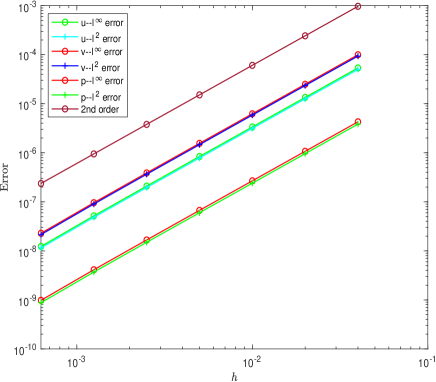
Case 1: a one-dimensional test with ϵO(1)similar-toitalic-ϵ𝑂1\epsilon\sim O(1). Consider the fast reaction–diffusion system (1)-(3). We first apply the first-order semi-implicit scheme to such model with the coefficients ϵ=1italic-ϵ1\epsilon=1 and the initial condition (4) and the Dirichlet boundary condition (59) given in the following form

v(x,0)=cos(πx2L)+ϵ0,u(x,0)=1v+ϵ0,p(x,0)=x2L+12,ϵ0=108,x[L,L],formulae-sequence𝑣𝑥0𝜋𝑥2𝐿subscriptitalic-ϵ0formulae-sequence𝑢𝑥01𝑣subscriptitalic-ϵ0formulae-sequence𝑝𝑥0𝑥2𝐿12formulae-sequencesubscriptitalic-ϵ0superscript108𝑥𝐿𝐿\displaystyle v(x,0)=\cos\left(\frac{\pi x}{2L}\right)+\epsilon_{0},\quad u(x,0)=1-v+\epsilon_{0},\quad p(x,0)=\frac{x}{2L}+\frac{1}{2},\quad\epsilon_{0}=10^{-8},\quad x\in[-L,L],
u(L,t)=u(L,t)=1,v(L,t)=v(L,t)=ϵ0.formulae-sequence𝑢𝐿𝑡𝑢𝐿𝑡1𝑣𝐿𝑡𝑣𝐿𝑡subscriptitalic-ϵ0\displaystyle u(-L,t)=u(L,t)=1,\quad v(-L,t)=v(L,t)=\epsilon_{0}.

In the first test, we verify the accuracy order of our scheme in both space and time. The computation domain is taken as [L,L],L=1𝐿𝐿𝐿1[-L,L],L=1, the results of the first-order convergence in time at t=0.1𝑡0.1t=0.1 are shown in Figure 1 (left) and Table 1, where we take the time step size τ=2jτ0,j=0,1,,9,10formulae-sequence𝜏superscript2𝑗subscript𝜏0𝑗01910\tau=2^{-j}\tau_{0},j=0,1,\cdots,9,10 with τ0=0.002subscript𝜏00.002\tau_{0}=0.002 and the spatial mesh size h=1.25×1021.25superscript102h=1.25\times 10^{-2}. In this test, the reference solution is obtained by taking h=1.25×1021.25superscript102h=1.25\times 10^{-2} and τ=213τ0𝜏superscript213subscript𝜏0\tau=2^{-13}\tau_{0}. Then Figure 1 (Right) and Table 2 show the second order convergence in space, where we take the uniform mesh size h=2jh0,j=0,1,,5,6formulae-sequencesuperscript2𝑗subscript0𝑗0156h=2^{-j}h_{0},j=0,1,\cdots,5,6 with h0=4×10²subscript04superscript102h_{0}=4\times 10^{-2} and τ=6.25×10³𝜏6.25superscript103\tau=6.25\times 10^{-3}. In this test, the solution on mesh with mesh size h=28h0,τ=6.25×10³formulae-sequencesuperscript28subscript0𝜏6.25superscript103h=2^{-8}h_{0},\tau=6.25\times 10^{-3} is regarded as the reference solution.
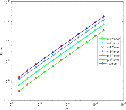
Refer to caption
Refer to caption
Figure 1: Left: First-order semi-implicit scheme: accuracy order check in τ𝜏\tau with ϵ=1italic-ϵ1\epsilon=1 and h=1.25×10²,τ=2jτ0,j=0,1,,9,10formulae-sequence1.25superscript102formulae-sequence𝜏superscript2𝑗subscript𝜏0𝑗01910h=1.25\times 10^{-2},\tau=2^{-j}\tau_{0},j=0,1,\cdots,9,10. Right: First-order semi-implicit scheme: accuracy order check in hh with ϵ=1italic-ϵ1\epsilon=1 and τ=6.25×10³,h=2jh0,j=0,1,,5,6formulae-sequence𝜏6.25superscript103formulae-sequencesuperscript2𝑗subscript0𝑗0156\tau=6.25\times 10^{-3},h=2^{-j}h_{0},j=0,1,\cdots,5,6.
Table 1: First-order semi-implicit scheme: accuracy order check in τ𝜏\tau with ϵ=1italic-ϵ1\epsilon=1, h=1.25×1021.25superscript102h=1.25\times 10^{-2}
τ𝜏\tau euτ,hsuperscriptsubscriptsubscript𝑒𝑢𝜏{e_{u}}_{\tau,h}^{\infty} order euτ,h2superscriptsubscriptsubscript𝑒𝑢𝜏2{e_{u}}_{\tau,h}^{2} order
1.9531e-05 6.1239e-07 5.8105e-07
3.9063e-05 1.3123e-06 1.0995 1.2451e-06 1.0995
7.8125e-05 2.7120e-06 1.0473 2.5732e-06 1.0473
1.5625e-04 5.5114e-06 1.0231 5.2294e-06 1.0231
3.1250e-04 1.1110e-05 1.0114 1.0542e-05 1.0114
6.2500e-04 2.2306e-05 1.0056 2.1165e-05 1.0056
1.2500e-03 4.4696e-05 1.0027 4.2409e-05 1.0027
2.5000e-03 8.9460e-05 1.0011 8.4884e-05 1.0011
5.0000e-03 1.7893e-04 1.0001 1.6979e-04 1.0001
1.0000e-02 3.5766e-04 0.99917 3.3939e-04 0.99923
1.0000e-02 7.1423e-04 0.99780 6.7781e-04 0.99793
Table 2: First-order semi-implicit scheme: accuracy order check in hh with ϵ=1italic-ϵ1\epsilon=1, τ=6.25×10³𝜏6.25superscript103\tau=6.25\times 10^{-3}
hh euτ,hsuperscriptsubscriptsubscript𝑒𝑢𝜏{e_{u}}_{\tau,h}^{\infty} order euτ,h2superscriptsubscriptsubscript𝑒𝑢𝜏2{e_{u}}_{\tau,h}^{2} order
6.2500e-04 1.2312e-08 1.1487e-08
1.2500e-03 5.1710e-08 2.0704 4.8248e-08 2.0704
2.5000e-03 2.0930e-07 2.0171 1.9529e-07 2.0171
5.0000e-03 8.3967e-07 2.0042 7.8345e-07 2.0042
1.0000e-02 3.3611e-06 2.0010 3.1361e-06 2.0010
2.0000e-02 1.3444e-05 1.9999 1.2546e-06 2.0002
4.0000e-02 5.3758e-05 1.9995 5.0180e-05 1.9999

Case 2: a one-dimensional test with ϵO(102)similar-toitalic-ϵ𝑂superscript102\epsilon\sim O(10^{-2}). We next consider the coefficients ϵ=102italic-ϵsuperscript102\epsilon=10^{-2}. The homogeneous Neumann boundary condition is considered at each boundary, and the initial condition (4) is given in the following form

u(x,0)={0,x<0,θd1,x>0,v(x,0)={Std2,x<0,0,x>0,p(x,0)={0,x<0,1,x>0,formulae-sequence𝑢𝑥0cases0𝑥0𝜃subscript𝑑1𝑥0formulae-sequence𝑣𝑥0casessubscript𝑆𝑡subscript𝑑2𝑥00𝑥0𝑝𝑥0cases0𝑥01𝑥0\displaystyle u(x,0)=\left\{\begin{array}[]{ll}0,&x<0,\\ \frac{\theta}{d_{1}},&x>0,\end{array}\right.\quad v(x,0)=\left\{\begin{array}[]{ll}\frac{S_{t}}{d_{2}},&x<0,\\ 0,&x>0,\end{array}\right.\quad p(x,0)=\left\{\begin{array}[]{ll}0,&x<0,\\ 1,&x>0,\end{array}\right. (111)

where θ=0.05,St=0.25,d1=1,d2=2formulae-sequence𝜃0.05formulae-sequencesubscript𝑆𝑡0.25formulae-sequencesubscript𝑑11subscript𝑑22\theta=0.05,S_{t}=0.25,d_{1}=1,d_{2}=2.

In this case, we verify the accuracy order of our scheme in time. The computation domain is taken as [L,L],L=1𝐿𝐿𝐿1[-L,L],L=1, the results of the first-order convergence in time at t=0.5𝑡0.5t=0.5 are shown in Figure 2 (left), where we take the time step size τ=2jτ0,j=0,1,,9,10formulae-sequence𝜏superscript2𝑗subscript𝜏0𝑗01910\tau=2^{-j}\tau_{0},j=0,1,\cdots,9,10 with τ0=0.01subscript𝜏00.01\tau_{0}=0.01 and the spatial mesh size h=1.25×1021.25superscript102h=1.25\times 10^{-2}. In this test, the reference solution is obtained by taking h=1.25×1021.25superscript102h=1.25\times 10^{-2} and τ=213τ0𝜏superscript213subscript𝜏0\tau=2^{-13}\tau_{0}.

Refer to caption
Refer to caption
Figure 2: Left: First-order semi-implicit scheme: accuracy order check in τ𝜏\tau with ϵ=102italic-ϵsuperscript102\epsilon=10^{-2} and h=1.25×10²,τ=2jτ0,j=0,1,,9,10formulae-sequence1.25superscript102formulae-sequence𝜏superscript2𝑗subscript𝜏0𝑗01910h=1.25\times 10^{-2},\tau=2^{-j}\tau_{0},j=0,1,\cdots,9,10. Right: Second-order semi-implicit Runge–Kutta scheme: accuracy order check in τ𝜏\tau with ϵ=102italic-ϵsuperscript102\epsilon=10^{-2} and h=6.25×10³,τ=2jτ0,j=0,1,,9,10formulae-sequence6.25superscript103formulae-sequence𝜏superscript2𝑗subscript𝜏0𝑗01910h=6.25\times 10^{-3},\tau=2^{-j}\tau_{0},j=0,1,\cdots,9,10.

4.1.2 Convergence test for the second-order semi-implicit Runge–Kutta scheme

Consider the coefficients ϵ=102italic-ϵsuperscript102\epsilon=10^{-2}. The initial and boundary condition is given in the following form

uϵ(x,0)=θd1,vϵ(x,0)=0,pϵ(x,0)=1,formulae-sequencesubscript𝑢italic-ϵ𝑥0𝜃subscript𝑑1formulae-sequencesubscript𝑣italic-ϵ𝑥00subscript𝑝italic-ϵ𝑥01\displaystyle u_{\epsilon}(x,0)=\frac{\theta}{d_{1}},\quad v_{\epsilon}(x,0)=0,\quad p_{\epsilon}(x,0)=1,
uϵ(L,t)=0,vϵ(L,t)=Std2,pϵ(L,t)=0,formulae-sequencesubscript𝑢italic-ϵ𝐿𝑡0formulae-sequencesubscript𝑣italic-ϵ𝐿𝑡subscript𝑆𝑡subscript𝑑2subscript𝑝italic-ϵ𝐿𝑡0\displaystyle u_{\epsilon}(-L,t)=0,\quad v_{\epsilon}(-L,t)=\frac{S_{t}}{d_{2}},\quad p_{\epsilon}(-L,t)=0,
uϵ(L,t)=θd1,vϵ(L,t)=0,pϵ(L,t)=1,formulae-sequencesubscript𝑢italic-ϵ𝐿𝑡𝜃subscript𝑑1formulae-sequencesubscript𝑣italic-ϵ𝐿𝑡0subscript𝑝italic-ϵ𝐿𝑡1\displaystyle u_{\epsilon}(L,t)=\frac{\theta}{d_{1}},\quad v_{\epsilon}(L,t)=0,\quad p_{\epsilon}(L,t)=1,

where d1=1subscript𝑑11d_{1}=1, d2=2subscript𝑑22d_{2}=2, λ=1𝜆1\lambda=1, θ=0.05𝜃0.05\theta=0.05, St=0.25subscript𝑆𝑡0.25S_{t}=0.25, L=1𝐿1L=1.

In this case, we verify the accuracy order in time of the semi-implicit Runge–Kutta scheme in Section 3. The computation domain is taken as [L,L]𝐿𝐿[-L,L], the results of the second-order convergence in time at t=0.5𝑡0.5t=0.5 are shown in Figure 2(Right), where we take the time step size τ=2jτ0,j=0,1,,9,10formulae-sequence𝜏superscript2𝑗subscript𝜏0𝑗01910\tau=2^{-j}\tau_{0},j=0,1,\cdots,9,10 with τ0=0.01subscript𝜏00.01\tau_{0}=0.01 and the spatial mesh size h=6.25×1036.25superscript103h=6.25\times 10^{-3}. In this test, the reference solution is obtained by taking h=6.25×1036.25superscript103h=6.25\times 10^{-3} and τ=213τ0𝜏superscript213subscript𝜏0\tau=2^{-13}\tau_{0}.

4.2 Limit behavior

4.2.1 One-dimensional case

In order to demonstrate the limit behavior of the fast reaction–diffusion system (1)-(3), we consider the following model with Dirichlet boundary conditions on the domain [L,L]×[0,T]𝐿𝐿0𝑇[-L,L]\times[0,T],

tuϵd1Δuϵ=1ϵuϵ[vϵ+λ(1pϵ)],subscript𝑡subscript𝑢italic-ϵsubscript𝑑1Δsubscript𝑢italic-ϵ1italic-ϵsubscript𝑢italic-ϵdelimited-[]subscript𝑣italic-ϵ𝜆1subscript𝑝italic-ϵ\displaystyle\partial_{t}u_{\epsilon}-d_{1}\Delta u_{\epsilon}=-\frac{1}{\epsilon}u_{\epsilon}[v_{\epsilon}+\lambda(1-p_{\epsilon})], (112)
tvϵd2Δvϵ=1ϵvϵ(uϵ+λpϵ),subscript𝑡subscript𝑣italic-ϵsubscript𝑑2Δsubscript𝑣italic-ϵ1italic-ϵsubscript𝑣italic-ϵsubscript𝑢italic-ϵ𝜆subscript𝑝italic-ϵ\displaystyle\partial_{t}v_{\epsilon}-d_{2}\Delta v_{\epsilon}=-\frac{1}{\epsilon}v_{\epsilon}(u_{\epsilon}+\lambda p_{\epsilon}),
tpϵ=1ϵ[(1pϵ)uϵvϵpϵ],subscript𝑡subscript𝑝italic-ϵ1italic-ϵdelimited-[]1subscript𝑝italic-ϵsubscript𝑢italic-ϵsubscript𝑣italic-ϵsubscript𝑝italic-ϵ\displaystyle\partial_{t}p_{\epsilon}=\frac{1}{\epsilon}[(1-p_{\epsilon})u_{\epsilon}-v_{\epsilon}p_{\epsilon}],
uϵ(x,0)=θd1,vϵ(x,0)=0,pϵ(x,0)=1,formulae-sequencesubscript𝑢italic-ϵ𝑥0𝜃subscript𝑑1formulae-sequencesubscript𝑣italic-ϵ𝑥00subscript𝑝italic-ϵ𝑥01\displaystyle u_{\epsilon}(x,0)=\frac{\theta}{d_{1}},\quad v_{\epsilon}(x,0)=0,\quad p_{\epsilon}(x,0)=1,
uϵ(L,t)=0,vϵ(L,t)=Std2,pϵ(L,t)=0,formulae-sequencesubscript𝑢italic-ϵ𝐿𝑡0formulae-sequencesubscript𝑣italic-ϵ𝐿𝑡subscript𝑆𝑡subscript𝑑2subscript𝑝italic-ϵ𝐿𝑡0\displaystyle u_{\epsilon}(-L,t)=0,\quad v_{\epsilon}(-L,t)=\frac{S_{t}}{d_{2}},\quad p_{\epsilon}(-L,t)=0,
uϵ(L,t)=θd1,vϵ(L,t)=0,pϵ(L,t)=1,formulae-sequencesubscript𝑢italic-ϵ𝐿𝑡𝜃subscript𝑑1formulae-sequencesubscript𝑣italic-ϵ𝐿𝑡0subscript𝑝italic-ϵ𝐿𝑡1\displaystyle u_{\epsilon}(L,t)=\frac{\theta}{d_{1}},\quad v_{\epsilon}(L,t)=0,\quad p_{\epsilon}(L,t)=1,

where d1=1subscript𝑑11d_{1}=1, d2=2subscript𝑑22d_{2}=2, λ=1𝜆1\lambda=1, θ=0.05𝜃0.05\theta=0.05, St=0.25subscript𝑆𝑡0.25S_{t}=0.25, L=1𝐿1L=1, T=1𝑇1T=1.

In this test, we first investigate the dynamic behavior of the solutions to the system (112). We first take ϵ=102italic-ϵsuperscript102\epsilon=10^{-2} and the mesh size h=0.01250.0125h=0.0125 and τ=5×10⁶𝜏5superscript106\tau=5\times 10^{-6}. Figure 3 shows the results of u,v,p𝑢𝑣𝑝u,v,p and the enthalpy function w𝑤w at time t𝑡t from 00 to 111. We can numerically check the positivity and bound preserving properties, which agrees with the numerical analysis in Section 2. Furthermore, as the strength of the reaction is much greater than that of the diffusion process, we can find that the increase or decrease of u𝑢u is consistent with p𝑝p, and the opposite is true for v𝑣v. Next we retake ϵ=104italic-ϵsuperscript104\epsilon=10^{-4}, Figure 4 shows the corresponding results with h=6.25×1036.25superscript103h=6.25\times 10^{-3} and τ=5×10⁶𝜏5superscript106\tau=5\times 10^{-6}. After comparing the dynamic behavior of the solutions with different ϵitalic-ϵ\epsilon, we can conclude that the smaller the ϵitalic-ϵ\epsilon the sharper the interface. The sharp interface is referred to as the phase transition interface in the limit Stefan problem, whose speed is determined by the Stefan’s condition. In this way, assume that the system is full of liquid at the initial moment, such as water, and give a freezing stimulus at the left edge of the system, then we can conclude that the liquid exothermizes and freezes, and the movement of the sharp interface moving to the right inscribes the liquid solidification process. Then Figure 5 shows more details on the sharp interface with various ϵitalic-ϵ\epsilon.

From Figure 6 we can conclude that for the first-order scheme, smaller parameters ϵitalic-ϵ\epsilon impose tighter requirements on the mesh size. Combined with the limit behavior, proposing an asymptotic preserving scheme on ϵitalic-ϵ\epsilon, which avoids the use of very fine meshes, is our future consideration.
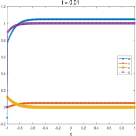
Refer to caption
Refer to caption
Refer to caption
Refer to caption
Refer to caption
Refer to caption
Refer to caption
Refer to caption
Refer to caption
Figure 3: First-order semi-implicit scheme with ϵ=102italic-ϵsuperscript102\epsilon=10^{-2} and h=0.0125,τ=5×10⁶formulae-sequence0.0125𝜏5superscript106h=0.0125,\tau=5\times 10^{-6}.
Refer to caption
Refer to caption
Refer to caption
Refer to caption
Refer to caption
Refer to caption
Refer to caption
Refer to caption
Refer to caption
Figure 4: First-order semi-implicit scheme: solutions u,v,p,w𝑢𝑣𝑝𝑤u,v,p,w with ϵ=104italic-ϵsuperscript104\epsilon=10^{-4} and h=6.25×1036.25superscript103h=6.25\times 10^{-3}, τ=5×10⁶𝜏5superscript106\tau=5\times 10^{-6}.
Refer to caption
Figure 5: First-order semi-implicit scheme: the enthalpy function w𝑤w at t=1𝑡1t=1 with various value of ϵitalic-ϵ\epsilon with τ=5×10⁶𝜏5superscript106\tau=5\times 10^{-6} and h=0.01250.0125h=0.0125.
Refer to caption
Refer to caption
Figure 6: First-order semi-implicit scheme: ewτ,h1superscriptsubscript𝑒subscript𝑤𝜏1e_{w_{\tau,h}}^{1} at t=1𝑡1t=1 with various value of ϵitalic-ϵ\epsilon, τ=0.01,0.005,0.0025,0.001,0.0005𝜏0.010.0050.00250.0010.0005\tau=0.01,0.005,0.0025,0.001,0.0005 and τ/h2=0.05𝜏superscript20.05\tau/h^{2}=0.05 where the reference solution is obtained by the fully-implicit method.

4.2.2 Two-dimensional case

In this test, we consider 𝒙=(x1,x2)[L,L]×[L,L]𝒙superscriptsubscript𝑥1subscript𝑥2𝐿𝐿𝐿𝐿\bm{x}=(x_{1},x_{2})^{\prime}\in[-L,L]\times[-L,L], 0tT0𝑡𝑇0\leq t\leqslant T. The initial condition (4) and Dirichlet boundary conditions (59) given in the following form,

uϵ(𝒙,0)subscript𝑢italic-ϵ𝒙0\displaystyle u_{\epsilon}(\bm{x},0) ={0,L<x10,θd1,0<x1<L,absentcases0𝐿subscript𝑥10𝜃subscript𝑑10subscript𝑥1𝐿\displaystyle=\left\{\begin{array}[]{ll}0,&-L<x_{1}\leq 0,\\ \frac{\theta}{d_{1}},&0<x_{1}<L,\end{array}\right. (115)
vϵ(𝒙,0)subscript𝑣italic-ϵ𝒙0\displaystyle v_{\epsilon}(\bm{x},0) ={θd2,L<x10,0,0<x1<L,absentcases𝜃subscript𝑑2𝐿subscript𝑥1000subscript𝑥1𝐿\displaystyle=\left\{\begin{array}[]{ll}\frac{\theta}{d_{2}},&-L<x_{1}\leq 0,\\ 0,&0<x_{1}<L,\end{array}\right. (118)
pϵ(𝒙,0)subscript𝑝italic-ϵ𝒙0\displaystyle p_{\epsilon}(\bm{x},0) ={0,Lx10,1,0<x1L,absentcases0𝐿subscript𝑥1010subscript𝑥1𝐿\displaystyle=\left\{\begin{array}[]{ll}0,&-L\leq x_{1}\leq 0,\\ 1,&0<x_{1}\leq L,\end{array}\right. (120)
uϵ(𝒙,t)|x1=Levaluated-atsubscript𝑢italic-ϵ𝒙𝑡subscript𝑥1𝐿\displaystyle u_{\epsilon}(\bm{x},t)|_{x_{1}=-L} =0,uϵ(𝒙,t)|x1=L=12(SmSt)x2+12(Sm+St),formulae-sequenceabsent0evaluated-atsubscript𝑢italic-ϵ𝒙𝑡subscript𝑥1𝐿12subscript𝑆𝑚subscript𝑆𝑡subscript𝑥212subscript𝑆𝑚subscript𝑆𝑡\displaystyle=0,\quad u_{\epsilon}(\bm{x},t)|_{x_{1}=L}=\frac{1}{2}(S_{m}-S_{t})x_{2}+\frac{1}{2}(S_{m}+S_{t}),
vϵ(𝒙,t)|x1=Levaluated-atsubscript𝑣italic-ϵ𝒙𝑡subscript𝑥1𝐿\displaystyle v_{\epsilon}(\bm{x},t)|_{x_{1}=-L} =12(SmSt)x2+12(Sm+St),vϵ(𝒙,t)x1=L=0,formulae-sequenceabsent12subscript𝑆𝑚subscript𝑆𝑡subscript𝑥212subscript𝑆𝑚subscript𝑆𝑡subscript𝑣italic-ϵsubscript𝒙𝑡subscript𝑥1𝐿0\displaystyle=-\frac{1}{2}(S_{m}-S_{t})x_{2}+\frac{1}{2}(S_{m}+S_{t}),\quad v_{\epsilon}(\bm{x},t)_{x_{1}=L}=0,

where d1=1subscript𝑑11d_{1}=1, d2=2subscript𝑑22d_{2}=2, λ=1𝜆1\lambda=1, St=0.25subscript𝑆𝑡0.25S_{t}=0.25, Sm=0.05subscript𝑆𝑚0.05S_{m}=0.05, L=1𝐿1L=1, T=3𝑇3T=3 and

θ(𝒙,0)={0.05,L<x1<0,0,x1=0,0.05,0<x1<L.𝜃𝒙0cases0.05𝐿subscript𝑥100subscript𝑥100.050subscript𝑥1𝐿\displaystyle\theta(\bm{x},0)=\left\{\begin{array}[]{ll}-0.05,&-L<x_{1}<0,\\ 0,&x_{1}=0,\\ 0.05,&0<x_{1}<L.\end{array}\right. (124)

Figure 7 and 8 give the results of the enthalpy function w𝑤w and the temperature θ=B(w)𝜃𝐵𝑤\theta=B(w) of the substance with ϵ=105italic-ϵsuperscript105\epsilon=10^{-5} and the mesh size Δx=0.05Δ𝑥0.05\Delta x=0.05, τ=0.001𝜏0.001\tau=0.001.

Refer to caption
Refer to caption
Refer to caption
Refer to caption
Figure 7: First-order semi-implicit scheme: w𝑤w with ϵ=105italic-ϵsuperscript105\epsilon=10^{-5} and h=0.05,τ=0.001formulae-sequence0.05𝜏0.001h=0.05,\tau=0.001.
Refer to caption
Refer to caption
Refer to caption
Refer to caption
Figure 8: First-order semi-implicit scheme: θ=B(w)𝜃𝐵𝑤\theta=B(w) with ϵ=105italic-ϵsuperscript105\epsilon=10^{-5} and h=0.05,τ=0.001formulae-sequence0.05𝜏0.001h=0.05,\tau=0.001.

5 Conclusions

In this paper, we study the semi-implicit strategy on the fast reaction–diffusion equations (1)-(4) and develop the semi-implicit schemes with first- and second-order accurate in time respectively. And our semi-implicit scheme preserves some analytical properties of the original model at the semi- and fully-discrete level. We also provide a series of numerical tests to demonstrate the properties, such as numerical convergence, non-negativity, and bound preserving, and to capture the movement of the sharp interface with various ϵitalic-ϵ\epsilon and to explore the heat transfer process, such as solid melting or liquid solidification.

Acknowledgements

The work of Z. Zhou was supported by the National Key R & D Program of China, Project Number 2020YFA0712000, and NSFC grant number 12031013, 12171013.

References

  • [1] R. Anguelov and J. M.-S. Lubuma. Contributions to the mathematics of the nonstandard finite difference method and applications. Numerical Methods for Partial Differential Equations: An International Journal, 17(5):518–543, 2001.
  • [2] G. Beckett, J. A. Mackenzie, and M. L. Robertson. A moving mesh finite element method for the solution of two-dimensional Stefan problems. Journal of Computational Physics, 168(2):500–518, 2001.
  • [3] S. Boscarino, F. Filbet, and G. Russo. High order semi-implicit schemes for time dependent partial differential equations. Journal of Scientific Computing, 68:975–1001, 2016.
  • [4] J. Caldwell and Y. Y. Kwan. Numerical methods for one-dimensional Stefan problems. Communications in numerical methods in engineering, 20(7):535–545, 2004.
  • [5] S. Chen, B. Merriman, S. Osher, and P. Smereka. A simple level set method for solving Stefan problems. Journal of Computational Physics, 135(1):8–29, 1997.
  • [6] S. M. Cox and P. C. Matthews. Exponential time differencing for stiff systems. Journal of Computational Physics, 176(2):430–455, 2002.
  • [7] A. W. Date. Novel strongly implicit enthalpy formulation for multidimensional Stefan problems. Numerical Heat Transfer, Part B Fundamentals, 21(2):231–251, 1992.
  • [8] F. Diele, M. Garvie, and C. Trenchea. Numerical analysis of a first-order in time implicit-symplectic scheme for predator–prey systems. Computers & Mathematics with Applications, 74(5):948–961, 2017.
  • [9] A. Esen and S. Kutluay. A numerical solution of the Stefan problem with a Neumann-type boundary condition by enthalpy method. Applied Mathematics and Computation, 148(2):321–329, 2004.
  • [10] J. Fernandez-Diaz and W. O. Williams. A generalized Stefan condition. Zeitschrift für angewandte Mathematik und Physik ZAMP, 30:749–755, 1979.
  • [11] D. Hilhorst, M. Mimura, and R. Schätzle. Vanishing latent heat limit in a Stefan-like problem arising in biology. Nonlinear analysis: real world applications, 4(2):261–285, 2003.
  • [12] D. Hilhorst, R. Van Der Hout, and L. A. Peletier. The fast reaction limit for a reaction–diffusion system. Journal of mathematical analysis and applications, 199(2):349–373, 1996.
  • [13] A. L. Hodgkin and A. F. Huxley. A quantitative description of membrane current and its application to conduction and excitation in nerve. The Journal of physiology, 117(4):500, 1952.
  • [14] D. Z. Huang, P.-O. Persson, and M. J. Zahr. High-order, linearly stable, partitioned solvers for general multiphysics problems based on implicit–explicit Runge–Kutta schemes. Computer Methods in Applied Mechanics and Engineering, 346:674–706, 2019.
  • [15] E. M. Izhikevich and R. FitzHugh. Fitzhugh-nagumo model. Scholarpedia, 1(9):1349, 2006.
  • [16] K. A. Johnson and R. S. Goody. The original michaelis constant: translation of the 1913 Michaelis–Menten paper. Biochemistry, 50(39):8264–8269, 2011.
  • [17] P. Kareiva. Population dynamics in spatially complex environments: theory and data. Philosophical Transactions of the Royal Society of London. Series B: Biological Sciences, 330(1257):175–190, 1990.
  • [18] A.-K. Kassam and L. N. Trefethen. Fourth-order time-stepping for stiff PDEs. SIAM Journal on Scientific Computing, 26(4):1214–1233, 2005.
  • [19] A. Q. M. Khaliq, J. Martin-Vaquero, B. A. Wade, and M. Yousuf. Smoothing schemes for reaction–diffusion systems with nonsmooth data. Journal of Computational and Applied Mathematics, 223(1):374–386, 2009.
  • [20] T. Koto. IMEX Runge–Kutta schemes for reaction–diffusion equations. Journal of Computational and Applied Mathematics, 215(1):182–195, 2008.
  • [21] S. Kutluay, A. R. Bahadir, and A. Özdeş. The numerical solution of one-phase classical Stefan problem. Journal of computational and applied mathematics, 81(1):135–144, 1997.
  • [22] J. A. Mackenzie and M. L. Robertson. The numerical solution of one-dimensional phase change problems using an adaptive moving mesh method. Journal of computational Physics, 161(2):537–557, 2000.
  • [23] A. Madzvamuse. Time-stepping schemes for moving grid finite elements applied to reaction–diffusion systems on fixed and growing domains. Journal of computational physics, 214(1):239–263, 2006.
  • [24] A. Madzvamuse and A. H. W. Chung. Fully implicit time-stepping schemes and non-linear solvers for systems of reaction–diffusion equations. Applied Mathematics and Computation, 244:361–374, 2014.
  • [25] R. McFadden and C. S. Kwok. Mathematical model of simultaneous diffusion and binding of antitumor antibodies in multicellular human tumor spheroids. Cancer research, 48(14):4032–4037, 1988.
  • [26] A. M. Meirmanov. The stefan problem, volume 3. Walter de Gruyter, 2011.
  • [27] R. E. Mickens. Nonstandard finite difference schemes: methodology and applications. World Scientific, 2020.
  • [28] B. Perthame. Parabolic equations in biology. Springer, 2015.
  • [29] J. Stefan. Über das gleichgewicht und die bewegung, insbesondere die diffusion von gasgemengen. Sitzungsberichte der Mathematisch-Naturwissenschaftlichen Classe der Kaiserlichen Akademie der Wissenschaften Wien, 63:63–124, 1871.
  • [30] M. Tong and D. J. Browne. Smoothed particle hydrodynamics modelling of the fluid flow and heat transfer in the weld pool during laser spot welding. IOP Conference Series: Materials Science and Engineering, 27(1):012080, 2012.
  • [31] J. J. Tyson. The belousov-zhabotinskii reaction, volume 10. Springer Science & Business Media, 2013.
  • [32] H. Wang, Q. Zhang, and C.-W. Shu. Third order implicit–explicit Runge–Kutta local discontinuous Galerkin methods with suitable boundary treatment for convection–diffusion problems with Dirichlet boundary conditions. Journal of Computational and Applied Mathematics, 342:164–179, 2018.
  • [33] P. J. Wangersky. Lotka-Volterra population models. Annual Review of Ecology and Systematics, 9(1):189–218, 1978.
  • [34] Z. Zhang, S. Ma, and Z. Zhou. Uncertainty quantification of phase transition problems with an injection boundary. arXiv preprint arXiv:2402.02806, 2024.