Semiparametric mean and variance joint models with Laplace link functions for count time series
Tianqing Liu∗
Center for Applied Statistical Research and School of Mathematics, Jilin University, China
tianqingliu@gmail.com
Xiaohui Yuan
School of Mathematics and Statistics, Changchun University of Technology, China
yuanxh@ccut.edu.cn
This version: \usdate
Abstract
Count time series data are frequently analyzed by modeling their conditional means and the conditional variance is often considered to be a deterministic function of the corresponding conditional mean and is not typically modeled independently. We propose a semiparametric mean and variance joint model, called random rounded count-valued generalized autoregressive conditional heteroskedastic (RRC-GARCH) model, to address this limitation. The RRC-GARCH model and its variations allow for the joint modeling of both the conditional mean and variance and offer a flexible framework for capturing various mean-variance structures (MVSs). One main feature of this model is its ability to accommodate negative values for regression coefficients and autocorrelation functions. The autocorrelation structure of the RRC-GARCH model using the proposed Laplace link functions with nonnegative regression coefficients is the same as that of an autoregressive moving-average (ARMA) process. For the new model, the stationarity and ergodicity are established and the consistency and asymptotic normality of the conditional least squares estimator are proved. Model selection criteria are proposed to evaluate the RRC-GARCH models. The performance of the RRC-GARCH model is assessed through analyses of both simulated and real data sets. The results indicate that the model can effectively capture the MVS of count time series data and generate accurate forecast means and variances.
Keywords:
Conditional mean, Conditional variance, Count time series, Integer-valued time series, Random rounding operator
1 Introduction
Gaussian models have been widely used for analyzing real-valued time series data. Because these models are completely characterized by their first two moments and and the conditional mean and variance can be modeled separately. However, Gaussian models often poorly described discrete-valued series. Various models (Kedem & Fokianos, 2002; Cameron & Trivedi, 2013; Wei, 2018) have been proposed for modeling discrete-valued data, taking into account their specific characteristics and distributions.
Integer-valued time series models have garnered increasing interest in recent years due to their applicability in various domains such as finance, economics, and telecommunications. These models are defined within the set of all integers, i.e., . Liu & Yuan (2013) showed a mean-variance structure (MVS) for all integer-valued data. Let be an integer-valued time series and be the -field generated by . The MVS is given by
| (1.1) |
where is a non-negative -measurable function and for ,
| (1.2) |
Thus, the inequality holds for all integer-valued time series. Integer-valued time series have other traits frequently observed in practice, such as overdispersion or underdispersion, excess of zeros or ones, asymmetry or symmetry of marginal distribution, and persistence (Wei, 2018). Numerous integer-valued models have been introduced so far to highlight the above nature of integer-valued time series. See Scotto et al. (2015), Karlis & Mamode (2023) and Li et al. (2024) for a comprehensive review for integer-valued models.
Count time series take values in and are important cases of integer-valued time series. Count time series arise in numerous applied scientific areas and usually count of some event in time and/or space. Originally, count series were often described via thinning operator (McKenzie, 1985, 2003) or regression type models (Davis et al., 2000, 2003; Davis & Wu, 2009; Kedem & Fokianos, 2002). As the field developed, various approaches for modeling count series emerged, such as the multiplicative error models (Heinen, 2003; Aknouche & Scotto, 2024; Wei & Zhu, 2024), the copula-based models (Jia et al., 2023; Kong & Lund, 2023), and the discrete mixed models (Gorgi, 2020; Chen et al., 2022; Maya et al., 2022). However, no single class of models dominates the count time series landscape and the field developed without a unifying statistical model, estimation method or inference theory.
All the above models are conditional mean-based models and the conditional variance is a deterministic function of the conditional mean. However, specifying the conditional MVS in a real data analysis can be challenging. While mean-based models are often easier to conceptualize and implement, accurately capturing the conditional variance adds another layer of complexity. In count time series analysis, the conditional MVS plays a central role in inference processes. However, due to the inherent complexities of real-world data, precisely defining this structure can be elusive. In practice, a misspecified MVS can indeed lead to significant inference errors. To deal with this problem, we first give two important properties of count random variables in the following proposition.
Proposition 1.1
(Count properties) Let be a count random variable taking values in such that the mean and variance exist. By Markov’s inequality, and for any and . Thus, : and : .
Obviously, count property can explain excess of zeros or ones of observations of with a small and property describes the MVSs of count random variables, which implies that, for a count random variable, its variance is controlled by its mean , when is small. In practice, one may apply the integer-valued models to analyze the count data. However, an ideal count model should not only preserve nonnegative characteristics but also adhere to properties and , thereby potentially offering superior fit or prediction for count time series data.
In the spirit of Box (1976), all models are wrong, but some are useful. A useful integer-valued or count-valued time series model should (a) be capable of capturing and generating a wide range of patterns within the time series data, (b) offer flexibility in the MVSs it can accommodate, (c) demonstrate its good predictive power when applied to real-world datasets. To account for these points, we propose a semiparametric count time series model, called RRC-GARCH. The main advantages of the new model can be summarized as follows.
-
(a)
The RRC-GARCH model offers a novel semiparametric framework to jointly model the conditional mean and variance for count time series.
-
(b)
Both the RRC-GARCH process with nonnegative regression coefficients and an ARMA process exhibit the same autocorrelation structure, where .
-
(c)
The RRC-GARCH model is more flexible than the existing models as its variants can provide various MVSs.
-
(d)
The RRC-GARCH model allows negative values both for its regression coefficients and autocorrelation function.
The rest of the paper is organized as follows. We first propose the RRC-GARCH model in Section 2. Then, in Section 3, we give theoretical results about the stationarity, ergodicity and autocorrelation structure of the RRC-GARCH process. Next, in Section 4, we prove the consistency and asymptotic normality of the conditional least squares estimator. In Section 5, we discuss the problem of model selection for the RRC-GARCH models. Simulations are presented in Section 6. In Section 7, applications of the model to two real data sets are discussed. Finally, we conclude the paper in Section 8. The proofs of all forthcoming results are postponed to the Section S1 of the Supplementary Material.
2 Background and the RRC-GARCH model
In the context of integer-valued time series, Liu & Yuan (2013) first proposed a semiparametric GARCH-type model to separately model the conditional mean and variance. In the following, we first give a simple review of the RRIN-GARCH models (Liu & Yuan, 2013; Li et al., 2024) and then propose our count model.
2.1 RRIN-GARCH model
Liu & Yuan (2013) proposed two random rounding operators. Let
with given in (1.2). The first-order and second-order random rounding operators are defined respectively as
| (2.1) | |||||
| (2.2) |
where is the indicator function of and is a uniform random variable defined on the interval . A RRIN-GARCH model is given as
| (2.3) |
where the variables , and , are mutually independent; and are two sequences of independent and identically distributed (i.i.d.) uniform random variables defined on the interval ; and is a sequence of i.i.d. integer-valued random variables with range , mean 0 and finite variance 1. Different assumptions on and lead to different integer-valued time series models (Liu & Yuan, 2013; Li et al., 2024). The MVS of RRIN-GARCH model is given in (1.1) with . However, the RRIN-GARCH model in (2.3) does not possess the nonnegative property and count properties in Proposition 1.1.
2.2 RRC-GARCH model
Let , be a count process, where ’s are (unbounded) count random variables with range . For , define as the ReLU activation function. Assume that satisfies the following iterative equation
| (2.4) |
where , , , is a specified link function satisfies that there exists a constant such that , for . Then, based on (2.4), we propose the following count time series model:
| (2.5) |
where , the first-order and second-order random rounding operators and are defined respectively in (2.1) and (2.2); is a sequence of i.i.d. count random variables with range , mean 1 and finite variance ; with and are i.i.d. uniform random variables defined on the interval ; and the variables , and , are mutually independent. We call this model RRC-GARCH. In the RRC-GARCH model (2.5), the unknown parameter vectors and determine the MVS of . However, the distribution of is not specified and remains nonparametric. In the following proposition, we present our findings on the basic properties of the RRC-GARCH models.
Proposition 2.2
The following equalities hold:
| (2.6) |
where the function is defined in (1.2) and
| (2.7) |
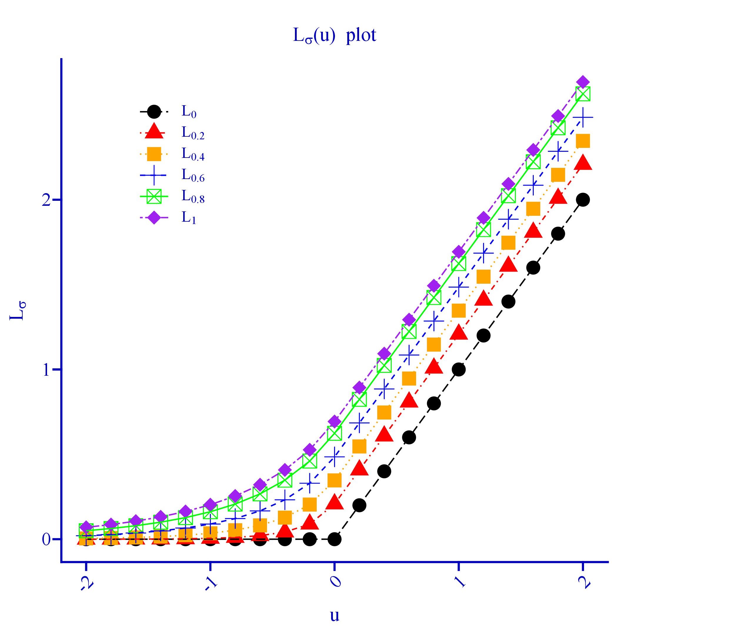
Moreover, for fixed , is a continuous increasing function of on ; for any fixed , is a non-decreasing function of on ; and for ; for and ; and for and . Overall, is a piecewise linear approximation of . In Figure 1, we present the plots of the functions with different values of .
Remark 2.1
A convenient choice for the link function is the ReLU activation function, i.e., . Other non-linear link specifications are also applicable for in (2.4), e.g., by adapting the softplus structure (Dugas et al., 2000; Mei Eisner,2017; Wei et al., 2022). The softplus function is given by , where and . In this paper, we propose the following Laplace link function:
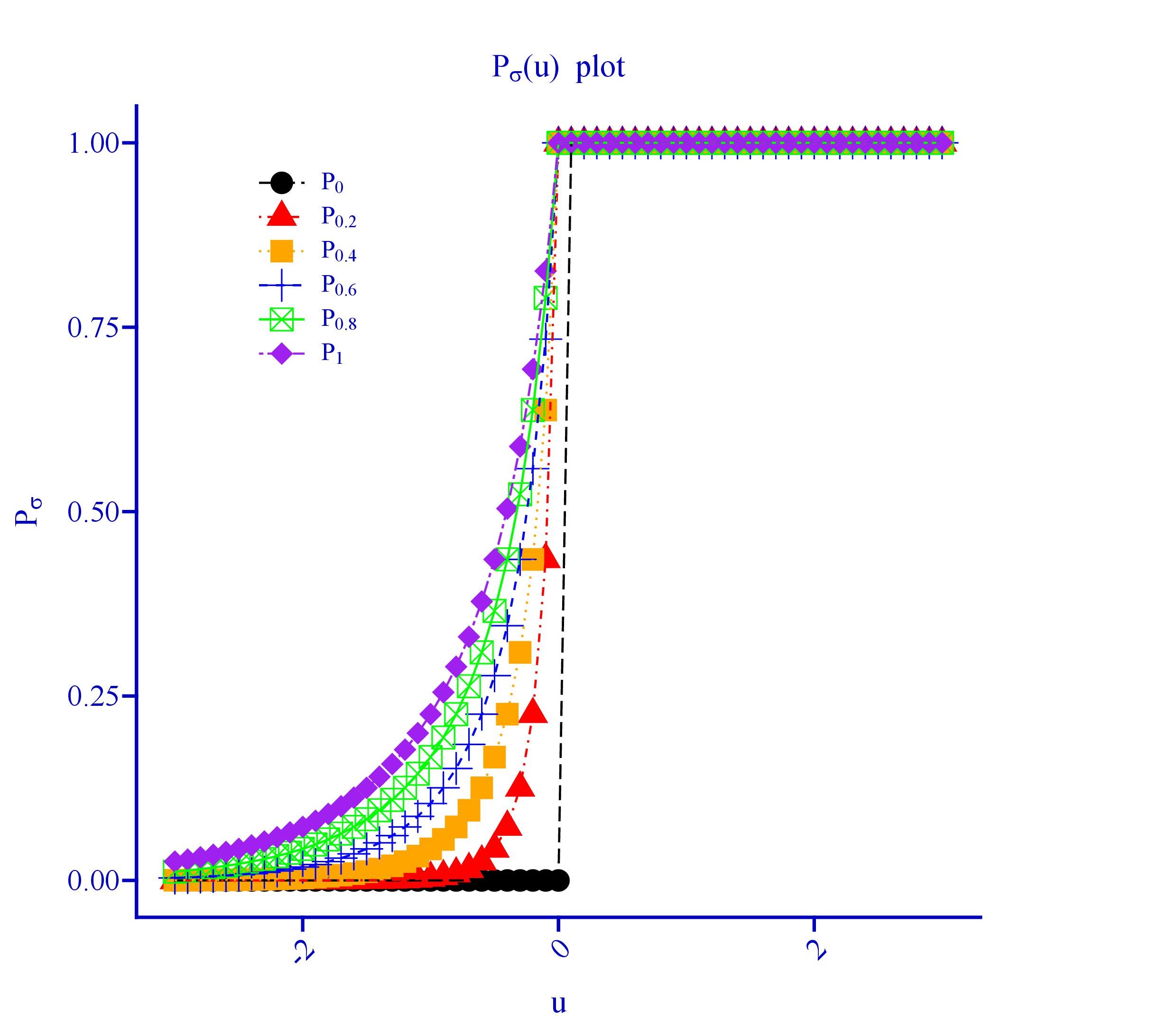
where is the standard Laplace cumulative distribution function (CDF) and is the default choice. It is easy to verify that and , where for and for . Thus, . In contrast to the softplus function, the Laplace link function with is linear for all . Moreover, is a truly positive and continuously differentiable function on whole , and it holds that , where is the standard Laplace density function. In Figures 2-3, we present the plots of the functions and with different values of . We stress that the the formula in (2.1) can generate a class of distribution link functions by setting as a CDF such that for . For example, if we set as the Logistic CDF, we obtain the softplus link function .
Remark 2.2
For , we consider two parameter spaces: and . Obvioulsy, . If , then . In this case, in (2.4) reduces to a linear function of . For , we consider the parameter space . For all , then is always a nonlinear function of .
Remark 2.3
The RRC-GARCH model involves the parameter vectors and . If we take the conditional mean function as the softplus or Laplace link function, then the parameter vector is identifiable if the conditional distribution of is not degenerate. Because and are strictly monotone increasing for . The identification of may be difficult. For example, if is small enough such that , then and can not be identifiable. However, and are always identifiable. We stress that the conditional mean and variance functions are our main interests and are identifiable if the conditional distribution of is not degenerate. Moreover, if and the conditional distribution of is not degenerate, then is identifiable.
Remark 2.4
(Extended RRC-GARCH) Let in (2.5), where is a -measurable function, e.g., or . Then, we obtain the extended MVS:
| (2.9) |
Remark 2.5
(Power RRC-GARCH) Using Jesen’s inequality, we have,
for ; and
for . Let in (2.5), we obtain the power MVS:
| (2.10) |
Remark 2.6
Remark 2.7
Similar to the proof of proposition 2.2, it is easy to verify that for the extended RRC-GARCH, power RRC-GARCH and mixture RRC-GARCH models. Moreover, Wei Zhu (2024) proposed a conditional-mean multiplicative error model (CMEM) with binomial multiplicative operator, whose MVS is , where and is the variance of the multiplicative error. Obviously, the power MVS (2.10) with and the mixture MVS (2.11) with and nest the MVS of the CMEM with binomial multiplicative operator as a special case. If and , we have , which is the MVS of a Bernoulli distribution with mean . By the definition of , we get . If or is large enough, the contribution of to is negligible in (2.10) and (2.11). In such a situation, the conditional variance in (2.11) is an approximation of , which contains the MVSs of Poisson and negative binomial distributions .
Remark 2.8
By the definitions of , , and , it is easy to verify that and , for . It follows that, for the RRC-GARCH, extended RRC-GARCH, power RRC-GARCH and mixture RRC-GARCH models: (1) and as ; (2) their conditional variances in (2.6), (2.9), (2.10) and (2.11) satisfy that as . In summary, the RRC-GARCH, extended RRC-GARCH, power RRC-GARCH and mixture RRC-GARCH models possess nonnegative property and count properties in Proposition 1.1.
Remark 2.9
For the RRC-GARCH, extended RRC-GARCH, power RRC-GARCH and mixture RRC-GARCH models, their MVSs have a unified expression
| (2.12) |
where for the RRC-GARCH, for the extended RRC-GARCH, for the power RRC-GARCH, and for the mixture RRC-GARCH. Here, we treat and as known terms. In Figures S1-S2 of the Supplementary Material, we present the plots of the functions for the power RRC-GARCH and mixture RRC-GARCH (r=1) with different values of .
3 Ergodicity, stationarity, autocorrelation structure and prediction
In this section, we study the stationary conditions, autocorrelation structure and prediction of the RRC-GARCH process.
3.1 Ergodicity and stationarity
Define
| (3.1) |
Then, the study of the RRC-GARCH process can be carried out through the following vectorized process
| (3.12) |
where . The process forms a homogeneous Markov chain with state space . For and , the transition probability function from to is given by
where , , for , and for .
The following proposition gives the conditions which ensure the ergodicity and the stationarity of the RRC-GARCH process. For , and any measure and function on , we set .
Proposition 3.3
Let and , where , for , for , and for . Suppose that:
-
1.
The Markov chain is irreducible and aperiodic;
-
2.
For some , ;
-
3.
, , for and ;
-
4.
.
Then
-
1.
The RRC-GARCH process has a unique invariant probability measure ;
-
2.
For all and , we have where denotes the conditional probability .
-
3.
.
Condition 1 is a necessary assumption for proving stationarity and ergodicity of a Markov chain. Condition 2 is a standard moment condition to guarantee that the conditional mean and variance of exist. Condition 3 is an essential condition for stationarity and ergodicity of a standard ARMA process. Note that, is a sufficient condition to ensure and for and . Condition 4 ensures the non-negative property of , . Since the constraints on the parameters of a stationary ergodic RRC-GARCH process are very weak, RRC-GARCH model can be applied to analyze more real count data sets.
Remark 3.10
The results in Proposition 3.3 depend on . From the proof of Proposition 3.3, we find that, the results in Proposition 3.3 still hold when , but require more stringent and complicated constraints on the parameters and . We do not intend to pursue this direction further. Since it is difficult to verify these complicated constraints on the parameters in a real data analysis.
3.2 Autocorrelation structure
Now, we show that the autocorrelation structure of a RRC-GARCH process with the proposed Laplace link function and is the same as that of a standard ARMA.
Let and . Then, define
From (2.4) and (2.1) and , it follows that
where
Let and recall that and . Then defined in (2.4) can be rewritten in terms of the backshift operator as . Note that for and implies that is well-defined for with some , where is exponentially decreasing and defined recursively and for . It follows that
| (3.14) |
where , .
Based on (2.5), (3.1) and (3.14), we can write
| (3.15) |
where and . From (3.15), we get
which gives
Finally, we obtain
| (3.16) | |||||
where , , and with .
If , then and the RRC-GARCH process can be written
| (3.17) | |||||
where with .
Let be the natural filtration associated to the RRC-GARCH process, where for , and is the degenerated -algebra. It is easy to see that and . From (3.16) and (3.17), we give the autocorrelation structure of the RRC-GARCH process in the following proposition .
Proposition 3.4
Suppose that and the conditions of Proposition 3.3 are satisfied. Let
then we have
where and satisfies with .
3.3 Prediction
For the RRC-GARCH type models, the one-step predictors of mean and variance are given respectively by
where
Note that the one-step predictors of mean and variance depend on the unknown parameter vectors and . To use these these one-step predictors, we need to plug in consistent estimates of these two unknown parameter vectors. In the next section, we will discuss the conditional least-squares estimation for the unknown parameters.
4 Conditional least-squares estimation
In this section, we state asymptotic results for the estimators of and . We consider the conditional least-squares estimator. The only requirement for an application of this method to model (2.5) or the other RRC-GARCH type models is the ergodicity of the solution. But since the Markov chain is ergodic, the ergodicity of the process easily follows.
Let be a stationary sequence of positive weights such that . For any , define
| (4.1) |
For model (2.5), the weighted least-squares (WLS) estimator of is given by
| (4.2) |
where and is a compact set of . If , is just the ordinary least squares (OLS) estimator of . In practice, minimization of (4.2) can be done by an approximation procedure. Let for . Then, can be approximated by
Correspondingly, can be approximated by the solution of
Theorem 4.1
Suppose that the conditions of Proposition 3.3 are satisfied. Furthermore, assume (i) implies that ; (ii)
| (4.3) |
Then, is strongly consistent, i.e. .
Theorem 4.2
Suppose that the conditions of Theorem 4.1 are satisfied. Assume furthermore that the sequence of weights satisfies
where is a neighborhood of and is the smallest eigenvalue of the matrix . Then, the WLS estimator is asymptotically normal, i.e.
where
Remark 4.11
The integrability conditions on the weights ensure that the matrices and and are well defined. It is well-known that the optimal choice of the weights for the asymptotic variance in the WLS estimation is given by
| (4.4) |
where
and is defined by (4.1).
If we want to apply the optimal weights in (4.4) to obtain a more efficient estimator of , we have to replace the unknown parameter vectors with an initial estimator, e.g., the OLS estimator . The following theorem justifies this two-steps procedure.
Theorem 4.3
Let be a sequence of estimators such that . Suppose that the conditions of Proposition 3.3 are satisfied. Moreover, assume
where and . Define the optimal WLS (OWLS) estimator of as
| (4.5) |
where with and . Then, we have where
For RRC-GARCH type models, OLS estimator of is given by
| (4.6) |
where and is a compact set of and is the OLS estimator of .
To solve , for fixed , define
It is easy to see that
The estimator can be computed by
We have the following result:
Theorem 4.4
Suppose that the conditions of Theorem 4.2 are satisfied. Furthermore, assume that (i) implies that ; (ii) , where is a neighborhood of . Then, is weakly consistent, i.e. .
Theorem 4.5
Suppose that the conditions of Theorem 4.4 are satisfied. Let . Furthermore, assume that
Then, the OLS estimator is asymptotically normal, i.e.
where is given in the proof of this theorem.
The algorithms for the computations of the OLS and OWLS estimates and their estimated asymptotic covariance matrices are provided in the Section S2 of the Supplementary Material.
5 Model selection and model diagnostics
5.1 Model selection
In this subsection, we consider the model selection problem for the RRC-GARCH models. Recall that is the OLS estimator of and is the OLS estimator of . Without specifying the distribution of in (2.5), the conditional likelihood function of the RRC-GARCH model can not be available. Following the idea of Hurvich & Tsai (1995) and Liu & Yuan (2013), we propose to use the conditional Gaussian quasi-likelihood to construct AIC and BIC for RRC-GARCH models. The resultant AIC and BIC are given respectively as
and
where and is given in (4.1).
Let be a maximum model order cut-offs for RRC-GARCH model. The selected order using AIC and BIC is given respectively by
and
We investigate the performances of these two criteria for selecting the RRC-GARCH models through simulations in the next section.
5.2 Model diagnostics
To check the adequacy of the conditional moments assumptions of RRC-GARCH models, we consider the standardized Pearson residuals , which are given by
where is the OLS estimate of and is the OLS or OWLS estimate of . For an adequate RRC-GARCH model, the Pearson residuals should have mean zero, variance one, and be uncorrelated. In particular, Aknouche & Scotto (2024) used the mean absolute residual (MAR), , and the mean squared Pearson residual, , for checking the adequacy of the dispersion structure. Obviously, smaller values of MAR and indicate a better model fit.
6 Simulation experiment
To evaluate the efficiency of the conditional least-squares estimators and the performances of the proposed AIC and BIC for selecting the RRC-GARCH models with the Laplace link function , we conduct two simulation studies. All simulations are carried out in the R Project for Statistical Computing. Moreover, in all simulations, the innovation variable, say , is generated from a Binomial distribution with parameter . Moreover, we set . Additional simulation results with or 0.8 presented in the Section S3 of the Supplementary Material yield similar results.
For the two Monte Carlo studies, we consider the following two settings:
-
Setting (a):
-
:
RRC-GARCH(1,0) model with ;
-
:
RRC-GARCH(1,1) model with ;
-
:
RRC-GARCH(1,2) model with ;
-
:
RRC-GARCH(2,0) model with ;
-
:
RRC-GARCH(2,1) model with ;
-
:
RRC-GARCH(2,2) model with ;
-
and Setting (b):
-
:
RRC-GARCH(1,0) model with ;
-
:
RRC-GARCH(1,1) model with ;
-
:
RRC-GARCH(1,2) model with ;
-
:
RRC-GARCH(2,0) model with ;
-
:
RRC-GARCH(2,1) model with ;
-
:
RRC-GARCH(2,2) model with .
To get an intuition about the abilities of the RRC-GARCH models with the Laplace link function for explaining different autocorrelation structures, we present sample ACF pairs for the above six RRC-GARCH models in Table 1. From Table 1, we see that, the RRC-GARCH models can exhibit different patterns of autocorrelation structures.
In the first simulation study, we use the root mean squared error (RMSE) to evaluate the finite sample behaviour of the conditional least squares estimators. We consider two sample sizes: and the number of replications is set to be . Simulation results for the settings (a) and (b) are presented in Tables 2-3, respectively. We find that the OWLS estimator gives smaller RMSEs for than the OLS estimator in most cases. Thus, the finite sample performance and the large sample asymptotic theory both show that the OWLS estimator is more efficient than the OLS estimator.
In the second Monte Carlo study, we examine the performances of AIC and BIC for selecting the RRC-GARCH models with the Laplace link function . We set the maximum model order cut-offs as (2,2). Thus, the set of candidate models is .
We consider three sample sizes: , and . Tables 4-5 give the numbers of the order selected by AIC and BIC in 1000 realizations. From the results reported in Tables 4-5, we find that AIC performs better than BIC in most cases for and , but BIC outperforms AIC in most cases when . Obviously, BIC tends to select a simpler model with small sample sizes while AIC tends to select a larger model. As the sample size increases from 100 to 500, both these two criteria perform very well according to the high probability for selecting the true model.
7 Applications to real data
To demonstrate how the RRC-GARCH models work, they are applied to two data sets in completely different areas.
7.1 Disease counts
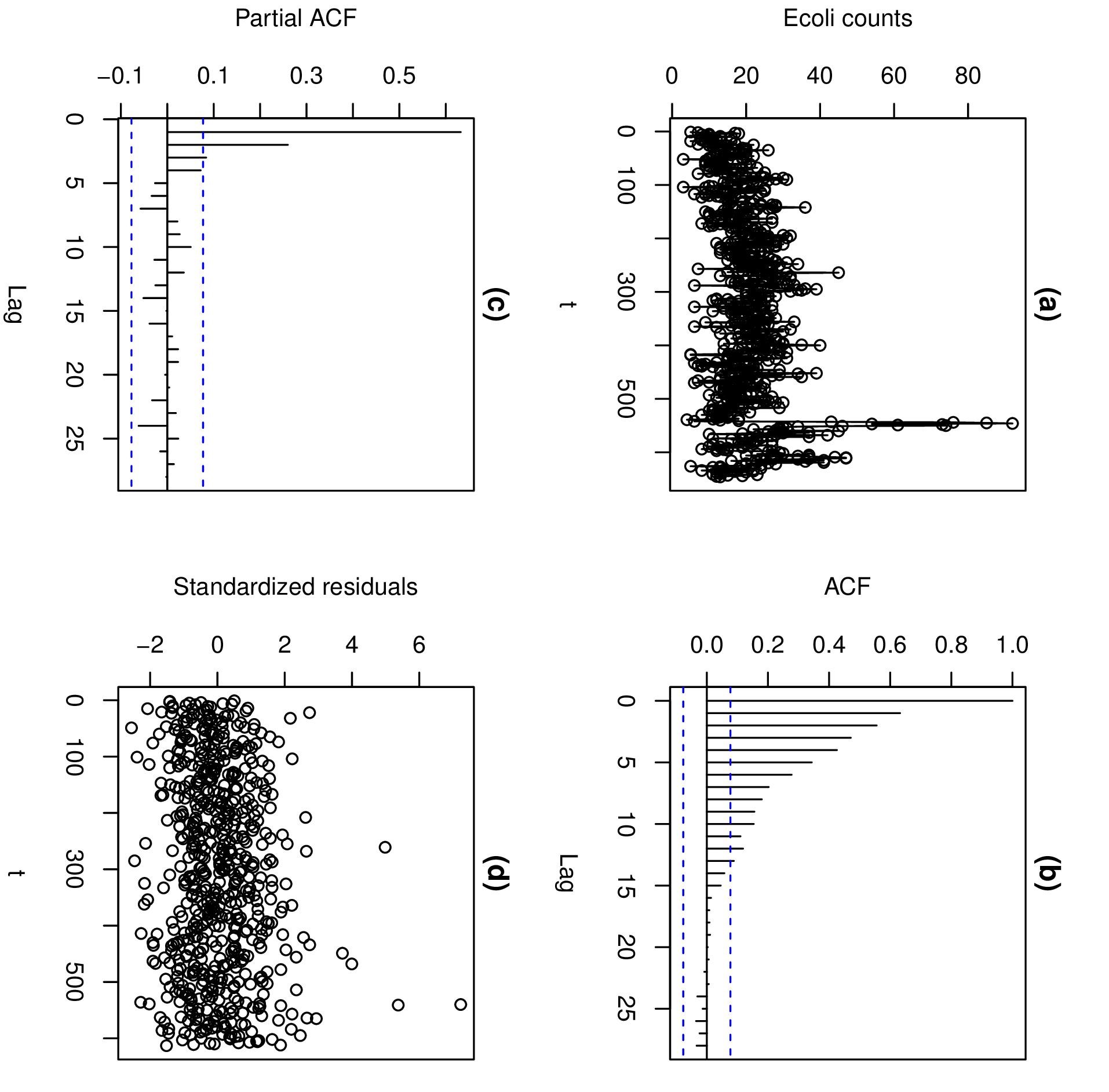
In this subsection, we consider the weekly counts of disease cases, which are caused by Escherichia coli (Ecoli) and reported for North Rhine-Westphalia (Germany) from January 2001 to May 2013.
These data were originally taken from SurvStat@RKI 2.0 at https://survstat .rki .de/ by Liboschik et al. (2017) and can be found via the command ecoli of the R-package tscount.
The length of the series is . The counts vary from 3 to 92 and its mean and variance is 20.3344 and 88.7531, respectively. Figure 4 (a, b, c) shows the plots of this time series, its sample autocorrelation (ACF) and sample partial autocorrelation (PACF). From Figure 4 (b,c), the PACF graph is truncated at the 2-th order, while the ACF graph is trailing. The sample ACF and PACF imply that the RRC-GARCH(2,0) model should be considered.
We use the first observations for fitting the RRC-GARCH models with the Laplace link function and leave out the last observations for a later forecast experiment. For model selection, we consider RRC-GARCH models with , , , , , and as candidate models. The AIC and BIC values of the candidate models for the Ecoli counts are given in Table 6. It is easy to see that both of these two criteria select the RRC-GARCH(2,0) model.
The final estimates together with their estimated standard deviations (SDs) are summarized in Table 7. Obviously, the OWLS estimate and the OLS estimate , which implies that the fitted RRC-GARCH(2,0) model has a linear mean structure. Moreover, the OWLS estimator gives smaller SDs for than the OLS estimator .
Figure 4(d) presented the standardized residuals plot using the OLS estimate of . To check the adequacy of the fitted models, we consider the approaches discussed in Section 5.2. The model diagnostics statistics MAR and MSPR with the OLS and OWLS estimates of are presented in Table 8. The sample means (), sample SDs (), and the maximum absolute value of the sample autocorrelation () of the standardized residuals using the OLS and OWLS estimates of are also reported. From Table 8, we see that, the OLS and OWLS methods have the same MAR values but the MSPR value of the OWLS method is closer to 1 than that of the OLS method using the RRC-GARCH(2,0) model, which indicates a better model fit.
Finally, let us analyze the forecast performance of the fitted RRC-GARCH(2,0) model with the OLS and OWLS estimates of . We apply the MAR and MSPR criteria to the 30 new Ecoli counts. The sample means (), sample SDs (), and the maximum absolute value of the sample autocorrelation () of the standardized prediction residuals using the OLS and OWLS estimates of are also considered. Results are summarized in Table 9. Obviously, the OWLS-fitted RRC-GARCH(2,0) model shows the better predictive performance regarding the 30 Ecoli counts, according to the MAR and MSPR criteria.
7.2 Transaction counts
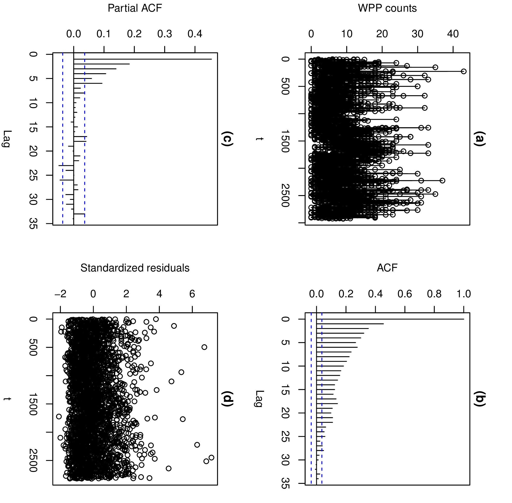
In the following, we shall investigate financial transactions counts data. Aknouche et al. (2022) provided one of the time series, i.e., the number of stock transactions concerning the Wausau Paper Corporation (WPP), measured in 5-min intervals between 9:45 AM and 4:00 PM for the period from January 3 to February 18 in 2005.
The length of the series is . The counts vary from 0 to 43 and its mean and variance is 8.1115 and 35.5382, respectively. Figure 5 (a, b, c) shows the plots of this time series, its sample autocorrelation (ACF) and sample partial autocorrelation (PACF). From Figure 5 (b,c), the PACF and ACF graphs are trailing. The sample ACF and PACF imply that the RRC-GARCH models with and should be considered.
In analogy to Aknouche et al. (2022, Section 6.2) and Wei & Zhu (2024, Section 6.2), we use the first observations for fitting the RRC-GARCH models with the Laplace link function and leave out the last observations for a later forecast experiment. For model selection, we consider RRC-GARCH models with , , , , , and as candidate models. The AIC and BIC values of the candidate models for the WPP counts are given in Table 6. Obviously, both of these two criteria select the RRC-GARCH(2,1) model.
The final estimates together with their estimated standard deviations (SDs) are summarized in Table 7. Obviously, the OWLS estimator and the OLS estimator , which implies that the fitted RRC-GARCH(2,1) model has a nonlinear mean structure. Moreover, the OWLS estimator gives smaller SDs for than the OLS estimator .
Figure 5(d) presents the standardized residuals plot using the OLS estimates of of . To check the adequacy of the fitted models, we also consider the approaches discussed in Section 5.2. The model diagnostics statistics MAR and MSPR with the OLS and OWLS estimates of are presented in Table 8. The sample means (), sample SDs (), and the maximum absolute value of the sample autocorrelation () of the standardized residuals using the OLS and OWLS estimates of are also reported. From Table 8, we see that, the OLS and OWLS methods have the same MAR values and similar MSPR values using the RRC-GARCH(2,1) model, which indicates a similar model fit.
Finally, let us evaluate the forecast performance of the fitted RRC-GARCH(2,1) model with the OLS and OWLS estimates of . We apply the MAR and MSPR criteria to the 100 new WPP counts. The sample means (), sample SDs (), and the maximum absolute value of the sample autocorrelation () of the standardized prediction residuals using the OLS and OWLS estimates of are also considered. Results are summarized in Table 9. Obviously, the OWLS-fitted RRC-GARCH(2,1) model shows the better predictive performance than the OLS-fitted RRC-GARCH(2,1) model regarding the 100 WPP counts, in terms of the MAR and MSPR criteria. Compared to the fitted CMEM model (MAR=3.613, MSPR=1.164) with Poi-counting series in Wei & Zhu (2024), the OWLS-fitted RRC-GARCH(2,1) model (MAR=3.5785, MSPR=1.1848) gives a smaller MAR value but a larger MSPR value. In summary, the OWLS-fitted RRC-GARCH(2,1) model shows the best predictive performance regarding the last 100 WPP counts, in terms of the MAR criterion.
8 Discussion
In this paper, we developed RRC-GARCH models for the analysis of count-valued time series. The RRC-GARCH model and its variants can provide flexible and feasible MVSs. The new model using the proposed Laplace link functions with an appropriate parameter space has a flexible range of ACF values and exhibits a linear mean structure, which makes its model parameters easier to interpret than those of a pure non-linear mean model. The OLS and OWLS estimators were used to estimate the model parameters, and their large-sample properties were derived. The proposed RRC-GARCH model offers a promising approach to jointly model the conditional mean and variance of count data. Its flexibility in handling different mean-variance structures and ability to provide efficient forecasts make it a valuable tool for analyzing count data.
In this paper, we only consider the conditional least-squares estimators of the regression parameters in the conditional mean and variance of the RRC-GARCH models, and the distribution of is not specified and remains nonparametric. We may consider the non-parametric maximum likelihood estimators (NPMLE) of and the distribution of in the RRC-GARCH model. Then, the NPMLE-based estimator of the forecast distribution may be obtained.
Supplementary Material
The online Supplementary Material contains the proofs of all Theorems, the detailed computation algorithm for the OLS and OWLS estimates and their estimated asymptotic covariance matrices, and additional simulation results.
Acknowledgements
We thank Professors Danning Li and Lianyan Fu for help discussions.
References
- 1 Aknouche, A., Almohaimeed, B. S. & Dimitrakopoulos, S. (2022) Forecasting transaction counts with integer-valued GARCH models. Studies in Nonlinear Dynamics & Econometrics 26: 529–539.
- 2 Aknouche, A. & Scotto, M. G. (2024) A multiplicative thinning-based integer-valued GARCH model. Journal of Time Series Analysis 45: 4–26.
- 3 Billingsley, P. (1968) Convergence of Probability Measures. New York: John Wiley.
- 4 Box, G. E. P. (1976) Science and statistics. Journal of the American Statistical Association 71 (356): 791–799.
- 5 Cameron, A. C. & Trivedi, P. K. (2013) Regression Analysis of Count Data. Cambridge, UK: Cambridge Univ. Press.
- 6 Chen, H., Li, Q. & Zhu, F. (2022) A new class of integer-valued GARCH models for time series of bounded counts with extra-binomial variation. AStA Advances in Statistical Analysis 106: 243–270.
- 7 Davis, R. A., Dunsmuir, W. T. M. & Wang, Y. (2000) On autocorrelation in a Poisson regression model. Biometrika 87, 491–505.
- 8 Davis, R. A., Dunsmuir, W. T. M. & Streett, S. B. (2003) Observation-driven models for Poisson counts. Biometrika 90, 777–790.
- 9 Davis, R. A. & Wu, R. (2009) A negative binomial model for time series of counts. Biometrika 96, 735–749.
- 10 Dugas, C., Bengio, Y., Bélisle, F., Nadeau, C. & Garcia, R. (2000) Incorporating second-order functional knowledge for better option pricing. In Proceedings of the 13th International Conference on Neural Information Processing Systems (NIPS’00) (Edited by Leen et al.), 451–457. MIT Press, Cambridge.
- 11 Heinen, A. (2003) Modeling Time Series Count Data: An Autoregressive Conditional Poisson Model. CORE Discussion Paper 2003/62, Université catholique de Louvain.
- 12 Hurvich, C. M. & Tsai, C. (1995) Model selection for extended quasi-likelihood models in small samples. Biometrics 51, 1077–1084.
- 13 Jia, Y., Kechagias, S., Livsey, J., Lund, R. & Pipiras, V. (2023) Latent Gaussian count time series. Journal of the American Statistical Association 118(541): 596–606.
- 14 Karlis, D. & Mamode Khan, N. M. (2023) Models for Integer Data. Annual Review of Statistics and Its Application 10: 297–323.
- 15 Kedem, B. & Fokianos, K. (2002) Regression Models for Time Series Analysis. Hoboken, New Jersey: Wiley.
- 16 Gorgi, P. (2020) Beta-negative binomial auto-regressions for modelling integer-valued time series with extreme observations. Journal of the Royal Statistical Society, Series B (Statistical Methodology) 82(5): 1325–1347.
- 17 Kong, J. & Lund, R. (2023) Seasonal count time series. Journal of Time Series Analysis 44(1): 93–124.
- 18 Li, Q., Chen, H. & Zhu, F. (2024) -valued time series: Models, properties and comparison. Journal of Statistical Planning and Inference 230:106099
- 19 Liboschik, T., Fokianos, K. & Fried, R. (2017) tscount: an R package for analysis of count time series following generalized linear models. Journal of Statistical Software 82: 1–51.
- 20 Liu, T. & Yuan, X. (2013) Random rounded integer-valued autoregressive conditional heteroskedastic process. Statistical Papers 54: 645–683.
- 21 Maya, R., Chesneau, C., Krishna, A. & Irshad, M. R. (2022) Poisson extended exponential distribution with associated INAR(1) process and applications. Statistics 5: 755-772.
- 22 McKenzie, E. (1985). Some simple models for discrete variate time series. Water Resources Bulletin 21(4), 645–650.
- 23 McKenzie, E. (2003) Discrete variate time series. In Handbook of Statistics 21: Stochastic Processes: Modeling and Simulation (eds C. R. Rao and D. N. Shanbhag). Amsterdam: Elsevier Science, pp. 573–606.
- 24 Mei, H. & Eisner, J. (2017) The neural Hawkes process: A neurally self-modulating multi- variate point process. In Proceedings of the 31st International Conference on Neural Infor- mation Processing Systems (NIPS’17) (Edited by von Luxburg et al.), Curran Associates Inc., 6757–6767.
- 25 Meyn, S. & Tweedie, R. L. (2009) Markov Chains and Stochastic Stability, second ed. Cambridge University Press, Cambridge.
- 26 Newey, W. K. & McFadden, D. (1994) Large sample estimation and hypothesis testing, in: R. Engle, D. McFadden (Eds.), Handbook of Econometrics, Vol. IV, Elsevier, Amsterdam, pp. 2111-2245.
- 27 Scotto, M. G., Wei, C. H. & Gouveia, S. (2015) Thinning-based models in the analysis of integer-valued time series: A review. Statistical Modelling 15(6): 590–618.
- 28 Wei, C. H. (2018) An Introduction to Discrete-Valued Time Series. John Wiley & Sons, Chichester.
- 29 Wei, C. H. & Zhu, F. (2024) Conditional-mean multiplicative operator models for count time series. Computational Statistics and Data Analysis 191, 107885
- 30 Wei, C. H., Zhu, F. & Hoshiyar, A. (2022) Softplus INGARCH models Statistica Sinica 32, 1099–1120.
- 31 Zheng, T., Xiao, H. & Chen, R. (2015) Generalized ARMA models with martingale difference errors. Journal of Econometrics 189: 492–506.
Table 1: ACF values for the simulated data.
| Setting | RRC-GARCH | |||||||
|---|---|---|---|---|---|---|---|---|
| (a) | 500 | 0.392 | 0.504 | 0.481 | 0.221 | 0.480 | 0.488 | |
| 0.180 | 0.445 | 0.331 | 0.406 | 0.647 | 0.650 | |||
| (b) | 500 | -0.497 | -0.458 | -0.392 | -0.169 | -0.100 | -0.062 | |
| 0.203 | 0.333 | 0.102 | -0.441 | -0.350 | -0.385 | |||
Table 2: Mean of estimates, RMSE (within parentheses) for the RRC-GARCH models with Laplace link function and under the setting (a).
| n | Method | ||||||||
|---|---|---|---|---|---|---|---|---|---|
| (1,0) | True Value | -0.4 | 0.5 | 0.5 | 0.5 | ||||
| 200 | OLS | -0.3947 | 0.4867 | 0.3250 | 0.5187 | ||||
| (0.1163) | (0.0955) | (0.3813) | (0.0864) | ||||||
| OWLS | -0.3970 | 0.4898 | |||||||
| (0.1140) | (0.0933) | ||||||||
| 500 | OLS | -0.3964 | 0.4918 | 0.4242 | 0.5084 | ||||
| (0.0731) | (0.0618) | (0.2984) | (0.0556) | ||||||
| OWLS | -0.3980 | 0.4939 | |||||||
| (0.0721) | (0.0607) | ||||||||
| (1,1) | True Value | -0.4 | 0.4 | 0.4 | 0.5 | 0.5 | |||
| 200 | OLS | -0.3272 | 0.4002 | 0.3507 | 0.4600 | 0.5186 | |||
| (0.1607) | (0.0750) | (0.1346) | (0.2163) | (0.1195) | |||||
| OWLS | -0.3346 | 0.4020 | 0.3545 | ||||||
| (0.1542) | (0.0733) | (0.1291) | |||||||
| 500 | OLS | -0.3740 | 0.4010 | 0.3818 | 0.4895 | 0.5063 | |||
| (0.0884) | (0.0471) | (0.0792) | (0.1387) | (0.0788) | |||||
| OWLS | -0.3758 | 0.4027 | 0.3813 | ||||||
| (0.0846) | (0.0444) | (0.0756) | |||||||
| (1,2) | True Value | -0.4 | 0.4 | 0.1 | 0.4 | 0.5 | 0.5 | ||
| 200 | OLS | -0.1106 | 0.4147 | 0.0957 | 0.2903 | 0.4606 | 0.5926 | ||
| (0.4604) | (0.0772) | (0.2325) | (0.2233) | (0.2105) | ( 0.2700) | ||||
| OWLS | -0.0872 | 0.4219 | 0.0938 | 0.2778 | |||||
| (0.4753) | (0.0762) | (0.2303) | (0.2251) | ||||||
| 500 | OLS | -0.3043 | 0.4109 | 0.0972 | 0.3601 | 0.4841 | 0.5370 | ||
| (0.1639) | (0.0466) | (0.1227) | (0.1169) | (0.1311) | (0.1556) | ||||
| OWLS | -0.2933 | 0.4158 | 0.0960 | 0.3530 | |||||
| (0.1711) | (0.0461) | (0.1169) | (0.1138) |
Table 2 (continued): Mean of estimates, RMSE (within parentheses) for the RRC-GARCH models with Laplace link function and under the setting (a).
| n | Method | ||||||||
|---|---|---|---|---|---|---|---|---|---|
| (2,0) | True Value | -0.4 | 0.2 | 0.5 | 0.5 | 0.5 | |||
| 200 | OLS | -0.3607 | 0.1858 | 0.4749 | 0.4141 | 0.5165 | |||
| (0.1263) | (0.0751) | (0.0798) | (0.2678) | (0.1002) | |||||
| OWLS | -0.3700 | 0.1890 | 0.4800 | ||||||
| (0.1255) | (0.0729) | (0.0785) | |||||||
| 500 | OLS | -0.3851 | 0.1962 | 0.4897 | 0.4629 | 0.5056 | |||
| (0.0809) | (0.0469) | (0.0522) | (0.1599) | (0.0619) | |||||
| OWLS | -0.3899 | 0.1978 | 0.4923 | ||||||
| (0.0782) | (0.0453) | (0.0499) | |||||||
| (2,1) | True Value | -0.4 | 0.1 | 0.4 | 0.4 | 0.5 | 0.5 | ||
| 200 | OLS | -0.2505 | 0.0967 | 0.4074 | 0.3430 | 0.4911 | 0.5405 | ||
| (0.2714) | (0.0745) | (0.0843) | (0.1373) | (0.1833) | (0.2091) | ||||
| OWLS | -0.2530 | 0.0989 | 0.4109 | 0.3388 | |||||
| (0.2670) | (0.0719) | (0.0806) | (0.1320) | ||||||
| 500 | OLS | -0.3450 | 0.1003 | 0.4017 | 0.3787 | 0.4891 | 0.5239 | ||
| (0.1211) | (0.0484) | (0.0567) | (0.0770) | (0.1074) | (0.1267) | ||||
| OWLS | -0.3467 | 0.1010 | 0.4052 | 0.3752 | |||||
| (0.1176) | (0.0451) | (0.0529) | (0.0738) | ||||||
| (2,2) | True Value | -0.4 | 0.1 | 0.4 | 0.1 | 0.3 | 0.5 | 0.5 | |
| 200 | OLS | -0.1432 | 0.1084 | 0.4065 | 0.0975 | 0.1981 | 0.4805 | 0.5547 | |
| (0.4056) | (0.0791) | (0.0786) | (0.2231) | (0.2076) | (0.1964) | (0.2314) | |||
| OWLS | -0.1402 | 0.1099 | 0.4084 | 0.0935 | 0.1985 | ||||
| (0.4094) | (0.0751) | (0.0760) | (0.2111) | (0.1996) | |||||
| 500 | OLS | -0.3140 | 0.1018 | 0.4064 | 0.1066 | 0.2563 | 0.4897 | 0.5221 | |
| (0.1620) | (0.0464) | (0.0467) | (0.1224) | (0.1151) | (0.1167) | (0.1343) | |||
| OWLS | -0.3122 | 0.1041 | 0.4087 | 0.1017 | 0.2564 | ||||
| (0.1587) | (0.0437) | (0.0441) | (0.1123) | (0.1084) |
Table 3: Mean of estimates, RMSE (within parentheses) for the RRC-GARCH models with Laplace link function and under the setting (b).
| n | Method | ||||||||
|---|---|---|---|---|---|---|---|---|---|
| (1,0) | True Value | 2.0 | -0.5 | 0.5 | 0.5 | ||||
| 200 | OLS | 2.0002 | -0.5022 | 0.5109 | 0.5097 | ||||
| (0.1520) | (0.0689) | (0.2361) | (0.1587) | ||||||
| OWLS | 1.9978 | -0.4999 | |||||||
| (0.1462) | (0.0633) | ||||||||
| 500 | OLS | 2.0007 | -0.5002 | 0.4969 | 0.5114 | ||||
| (0.0955) | (0.0425) | (0.1599) | (0.1110) | ||||||
| OWLS | 2.0005 | -0.4999 | |||||||
| (0.0920) | (0.0398) | ||||||||
| (1,1) | True Value | 2.0 | -0.4 | -0.4 | 0.5 | 0.5 | |||
| 200 | OLS | 1.9591 | -0.4135 | -0.3659 | 0.4831 | 0.5071 | |||
| (0.1920) | (0.0826) | (0.1334) | (0.2370) | (0.1304) | |||||
| OWLS | 1.9591 | -0.4104 | -0.3676 | ||||||
| (0.1869) | (0.0787) | (0.1316) | |||||||
| 500 | OLS | 1.9824 | -0.4072 | -0.3835 | 0.5012 | 0.4990 | |||
| (0.1110) | (0.0490) | (0.0790) | (0.1623) | (0.0866) | |||||
| OWLS | 1.9837 | -0.4055 | -0.3852 | ||||||
| (0.1078) | (0.0467) | (0.0765) | |||||||
| (1,2) | True Value | 2.0 | -0.4 | -0.1 | -0.4 | 0.5 | 0.5 | ||
| 200 | OLS | 1.8010 | -0.4200 | -0.0365 | -0.3126 | 0.4677 | 0.5041 | ||
| (0.4313) | (0.0793) | (0.1736) | (0.1921) | (0.2598) | (0.1194) | ||||
| OWLS | 1.8745 | -0.4141 | -0.0617 | -0.3421 | |||||
| (0.4210) | (0.0755) | (0.1810) | (0.1804) | ||||||
| 500 | OLS | 1.9454 | -0.4057 | -0.0814 | -0.3777 | 0.4840 | 0.5040 | ||
| (0.2451) | (0.0480) | (0.1031) | (0.1025) | (0.1863) | (0.0873) | ||||
| OWLS | 1.9545 | -0.4043 | -0.0842 | -0.3817 | |||||
| (0.2378) | (0.0461) | (0.1022) | (0.0988) |
Table 3 (continued): Mean of estimates, RMSE (within parentheses) for the RRC-GARCH models with Laplace link function and under the setting (b).
| n | Method | ||||||||
|---|---|---|---|---|---|---|---|---|---|
| (2,0) | True Value | 2.0 | -0.2 | -0.5 | 0.5 | 0.5 | |||
| 200 | OLS | 2.0143 | -0.2021 | -0.5066 | 0.4961 | 0.5018 | |||
| (0.1955) | (0.0662) | (0.0723) | (0.2500) | (0.1413) | |||||
| OWLS | 2.0115 | -0.2021 | -0.5040 | ||||||
| (0.1881) | (0.0635) | (0.0677) | |||||||
| 500 | OLS | 2.0031 | -0.2003 | -0.5030 | 0.4965 | 0.5037 | |||
| (0.1216) | (0.0400) | (0.0458) | (0.1650) | (0.0935) | |||||
| OWLS | 1.9999 | -0.1994 | -0.5016 | ||||||
| (0.1162) | (0.0382) | (0.0430) | |||||||
| (2,1) | True Value | 2.0 | -0.1 | -0.4 | -0.4 | 0.5 | 0.5 | ||
| 200 | OLS | 1.9343 | -0.1122 | -0.4074 | -0.3395 | 0.4607 | 0.5121 | ||
| (0.3210) | (0.0735) | (0.0725) | (0.1987) | (0.2744) | (0.1295) | ||||
| OWLS | 1.9488 | -0.1112 | -0.4059 | -0.3503 | |||||
| (0.3171) | (0.0720) | (0.0704) | (0.1958) | ||||||
| 500 | OLS | 1.9797 | -0.1027 | -0.4021 | -0.3830 | 0.4903 | 0.5010 | ||
| (0.1733) | (0.0436) | (0.0440) | (0.1035) | (0.1860) | (0.0838) | ||||
| OWLS | 1.9806 | -0.1021 | -0.4010 | -0.3846 | |||||
| (0.1683) | (0.0428) | (0.0424) | (0.1007) | ||||||
| (2,2) | True Value | 2.0 | -0.1 | -0.4 | -0.1 | -0.3 | 0.5 | 0.5 | |
| 200 | OLS | 1.9230 | -0.1077 | -0.4117 | -0.0711 | -0.2628 | 0.4685 | 0.5040 | |
| (0.3051) | (0.0761) | (0.0886) | (0.1579) | (0.1766) | (0.2479) | (0.1225) | |||
| OWLS | 1.9318 | -0.1074 | -0.4056 | -0.0725 | -0.2714 | ||||
| (0.3047) | (0.0747) | (0.0873) | (0.1598) | (0.1764) | |||||
| 500 | OLS | 1.9749 | -0.1048 | -0.4051 | -0.0885 | -0.2855 | 0.4833 | 0.5020 | |
| (0.1705) | (0.0462) | (0.0512) | (0.0964) | (0.0962) | (0.1649) | (0.0796) | |||
| OWLS | 1.9763 | -0.1032 | -0.4039 | -0.0910 | -0.2863 | ||||
| (0.1645) | (0.0441) | (0.0498) | (0.0925) | (0.0951) |
Table 4 : Frequency of orders selected by AIC and BIC for the RRC-GARCH models with Laplace link function and in 1000 realizations under the setting (a).
| Model | n | |||||||
|---|---|---|---|---|---|---|---|---|
| (1,0) | (1,1) | (1,2) | (2,0) | (2,1) | (2,2) | |||
| 100 | AIC | 453 | 128 | 130 | 105 | 93 | 91 | |
| BIC | 755 | 75 | 64 | 52 | 37 | 17 | ||
| 200 | AIC | 490 | 115 | 129 | 89 | 105 | 72 | |
| BIC | 803 | 55 | 46 | 46 | 37 | 13 | ||
| 500 | AIC | 545 | 129 | 101 | 66 | 104 | 55 | |
| BIC | 878 | 46 | 13 | 29 | 30 | 4 | ||
| 100 | AIC | 246 | 301 | 113 | 197 | 57 | 86 | |
| BIC | 504 | 214 | 45 | 193 | 22 | 22 | ||
| 200 | AIC | 78 | 444 | 116 | 247 | 37 | 78 | |
| BIC | 254 | 423 | 35 | 268 | 8 | 12 | ||
| 500 | AIC | 3 | 562 | 108 | 163 | 60 | 104 | |
| BIC | 25 | 698 | 24 | 237 | 8 | 8 | ||
| 100 | AIC | 224 | 263 | 271 | 82 | 64 | 96 | |
| BIC | 485 | 273 | 110 | 75 | 26 | 31 | ||
| 200 | AIC | 46 | 282 | 454 | 23 | 65 | 130 | |
| BIC | 190 | 437 | 279 | 39 | 36 | 19 | ||
| 500 | AIC | 0 | 65 | 683 | 0 | 43 | 209 | |
| BIC | 9 | 225 | 703 | 1 | 43 | 19 | ||
| 100 | AIC | 6 | 29 | 47 | 581 | 159 | 178 | |
| BIC | 24 | 32 | 28 | 785 | 65 | 66 | ||
| 200 | AIC | 1 | 4 | 20 | 635 | 151 | 189 | |
| BIC | 3 | 5 | 13 | 890 | 49 | 40 | ||
| 500 | AIC | 0 | 0 | 2 | 656 | 179 | 163 | |
| BIC | 0 | 1 | 1 | 933 | 44 | 21 | ||
| 100 | AIC | 0 | 49 | 60 | 356 | 368 | 167 | |
| BIC | 7 | 79 | 49 | 591 | 222 | 52 | ||
| 200 | AIC | 0 | 5 | 50 | 98 | 670 | 177 | |
| BIC | 0 | 28 | 48 | 308 | 573 | 43 | ||
| 500 | AIC | 0 | 0 | 7 | 6 | 789 | 198 | |
| BIC | 0 | 2 | 6 | 19 | 943 | 30 | ||
| 100 | AIC | 2 | 45 | 41 | 445 | 261 | 206 | |
| BIC | 13 | 78 | 33 | 686 | 151 | 39 | ||
| 200 | AIC | 0 | 15 | 20 | 176 | 378 | 411 | |
| BIC | 0 | 41 | 15 | 484 | 340 | 120 | ||
| 500 | AIC | 0 | 0 | 4 | 7 | 155 | 834 | |
| BIC | 0 | 1 | 4 | 84 | 405 | 506 | ||
Table 5 : Frequency of orders selected by AIC and BIC for the RRC-GARCH models with Laplace link function and in 1000 realizations under the setting (b).
| Model | n | |||||||
|---|---|---|---|---|---|---|---|---|
| (1,0) | (1,1) | (1,2) | (2,0) | (2,1) | (2,2) | |||
| 100 | AIC | 578 | 117 | 103 | 122 | 32 | 48 | |
| BIC | 852 | 45 | 32 | 63 | 4 | 4 | ||
| 200 | AIC | 640 | 93 | 81 | 116 | 42 | 28 | |
| BIC | 903 | 27 | 15 | 49 | 5 | 1 | ||
| 500 | AIC | 591 | 110 | 110 | 133 | 34 | 22 | |
| BIC | 932 | 26 | 7 | 35 | 0 | 0 | ||
| 100 | AIC | 289 | 290 | 185 | 171 | 35 | 30 | |
| BIC | 552 | 221 | 61 | 152 | 9 | 5 | ||
| 200 | AIC | 86 | 446 | 196 | 182 | 57 | 33 | |
| BIC | 291 | 440 | 62 | 183 | 19 | 5 | ||
| 500 | AIC | 3 | 564 | 202 | 123 | 70 | 38 | |
| BIC | 34 | 739 | 49 | 154 | 22 | 2 | ||
| 100 | AIC | 433 | 54 | 223 | 122 | 30 | 138 | |
| BIC | 761 | 16 | 99 | 87 | 8 | 29 | ||
| 200 | AIC | 295 | 7 | 459 | 74 | 23 | 142 | |
| BIC | 673 | 2 | 244 | 43 | 9 | 29 | ||
| 500 | AIC | 56 | 1 | 753 | 11 | 15 | 164 | |
| BIC | 300 | 0 | 648 | 17 | 8 | 27 | ||
| 100 | AIC | 0 | 11 | 39 | 616 | 184 | 150 | |
| BIC | 1 | 13 | 23 | 854 | 78 | 31 | ||
| 200 | AIC | 0 | 0 | 2 | 688 | 160 | 150 | |
| BIC | 0 | 0 | 2 | 929 | 50 | 19 | ||
| 500 | AIC | 0 | 0 | 0 | 729 | 158 | 113 | |
| BIC | 0 | 0 | 0 | 965 | 30 | 5 | ||
| 100 | AIC | 4 | 15 | 46 | 417 | 335 | 183 | |
| BIC | 22 | 22 | 35 | 672 | 204 | 45 | ||
| 200 | AIC | 0 | 3 | 11 | 247 | 572 | 167 | |
| BIC | 1 | 2 | 7 | 542 | 410 | 38 | ||
| 500 | AIC | 0 | 0 | 24 | 48 | 734 | 194 | |
| BIC | 0 | 0 | 24 | 220 | 729 | 27 | ||
| 100 | AIC | 2 | 7 | 41 | 577 | 95 | 278 | |
| BIC | 5 | 9 | 31 | 809 | 39 | 107 | ||
| 200 | AIC | 0 | 1 | 9 | 407 | 92 | 491 | |
| BIC | 0 | 1 | 8 | 769 | 39 | 183 | ||
| 500 | AIC | 0 | 0 | 0 | 99 | 39 | 862 | |
| BIC | 0 | 0 | 1 | 474 | 26 | 499 | ||
Table 6: AIC and BIC values for the real data.
| Data | RRC-GARCH | |||||||
|---|---|---|---|---|---|---|---|---|
| (1,0) | (1,1) | (1,2) | (2,0) | (2,1) | (2,2) | |||
| Ecoli counts | 616 | AIC | 2369.850 | 2289.293 | 2283.812 | 2280.248 | 2283.892 | 2283.049 |
| BIC | 2387.523 | 2311.385 | 2310.312 | 2302.331 | 2310.393 | 2313.966 | ||
| WPP counts | 2825 | AIC | 9088.451 | 8880.538 | 8833.220 | 8937.021 | 8811.859 | 8818.571 |
| BIC | 9112.231 | 8910.264 | 8868.889 | 8966.746 | 8847.528 | 8860.185 | ||
Table 7: Estimates and their estimated standard deviations (in parentheses) for the real data.
| Data | Model | Estimate | |||||||
|---|---|---|---|---|---|---|---|---|---|
| Ecoli counts | 616 | (2,0) | OLS | 4.8473 | 0.4833 | 0.2468 | 0.9999 | 0.1039 | |
| (1.3041) | (0.0796) | (0.0692) | (0.0955) | (0.0688) | |||||
| OWLS | 6.5702 | 0.3983 | 0.2442 | ||||||
| (0.8509) | (0.0588) | (0.0480) | |||||||
| WPP counts | 2825 | (2,1) | OLS | -0.1794 | 0.3162 | -0.1271 | 0.7478 | 0.6845 | 1.3986 |
| (0.1077) | (0.0253) | (0.0333) | (0.0335) | (0.0796) | (0.4956) | ||||
| OWLS | -0.1501 | 0.3111 | -0.1069 | 0.7294 | |||||
| (0.1061) | (0.0212) | (0.0301) | (0.0331) |
Table 8: Model diagnostics of the real data. Sample mean of the standardized residuals: ; Sample SD of the standardized residuals: ; the maximum absolute value of the sample autocorrelation: .
| Data | Model | Method | MAR | MSPR | ||||
|---|---|---|---|---|---|---|---|---|
| Ecoli counts | 616 | (2,0) | OLS | 0.0222 | 1.0824 | 0.134 | 5.2357 | 1.1702 |
| OWLS | 0.0034 | 1.0593 | 0.097 | 5.2357 | 1.1203 | |||
| WPP counts | 2825 | (2,1) | OLS | 0.0007 | 1.0345 | 0.062 | 3.9003 | 1.0697 |
| OWLS | 0.0005 | 1.0348 | 0.062 | 3.9003 | 1.0704 |
Table 9: Predictions of the real data.
| Data | Model | Method | MAR | MSPR | ||||
|---|---|---|---|---|---|---|---|---|
| Ecoli counts | 30 | (2,0) | OLS | -0.1000 | 1.1125 | 0.441 | 5.3518 | 1.2065 |
| OWLS | -0.1434 | 1.0623 | 0.426 | 5.2252 | 1.1114 | |||
| WPP counts | 100 | (2,1) | OLS | 0.0179 | 1.0962 | 0.320 | 3.5827 | 1.1899 |
| OWLS | 0.0165 | 1.0939 | 0.322 | 3.5785 | 1.1848 |