Photo-dynamical Analysis of Circumbinary Multi-planet system TOI-1338: a Fully Coplanar Configuration with a Puffy Planet
Abstract
TOI-1338 is the first circumbinary planet system discovered by TESS. It has one transiting planet at P95 day and an outer non-transiting planet at P215 day complemented by RV observation. Here we present a global photo-dynamical modeling of TOI-1338 system that self-consistently accounts for the mutual gravitational interactions between all known bodies in the system. As a result, the three-dimensional architecture of the system can be established by comparing the model with additional data from TESS Extended Mission and published HARPS/ESPRESSO radial velocity data. We report an inconsistency of binary RV signal between HARPS and ESPRESSO, which could be due to the contamination of the secondary star. According to stability analysis, the RV data via ESPRESSO is preferred. Our results are summarized as follows: (1) the inner transiting planet is extremely coplanar to the binary plane , making it a permanently transiting circumbinary planet at any nodal precession phases. We updated the future transit ephemerides with improved precisions. (2) The outer planet, despite its untransiting nature, is also coplanar with binary plane by (22∘ for 99% upper limit). (3) The inner planet could have a density extremely low as g/cm-3. With a TESS magnitude of 11.45, TOI-1338 b is an optimal circumbinary planet for ground-based follow-up and transit spectroscopy.
1 Introduction
Planets orbiting around both of the stars in binary systems are called the circumbinary planets (CBPs). Over the years the detections of CBPs mainly came from transit surveys like Kepler and TESS (e.g., Doyle et al., 2011a; Welsh et al., 2012, 2015; Kostov et al., 2020, 2021). Subject to the observational bias of the transit method, most confirmed CBPs are coplanar with their host binary orbital planes within and close-in (with semi-major axis around 1-2 times of system inner stability limit). Knowing the inclination distribution is essential to understanding the population and occurrence rates of the CBP population (Li et al., 2016; Martin, 2019). More faraway and misaligned CBPs are harder to detect with transit photometry, as it will produce irregular transit patterns (Martin & Triaud, 2014; Chen & Kipping, 2021). However, CBPs elude transiting might dynamically perturb the binary and showcase eclipsing binary variations (ETVs) as potential evidence of their existence (e.g., Qian et al., 2012; Er et al., 2021; Esmer et al., 2022), but such claims are sometimes debated (Pulley et al., 2022). Recent radial velocity surveys may expedite the discovery of more misaligned circumbinary planets (Standing et al., 2022). For example, the BEBPOP survey contributes to the discovery of TOI-1338 c (Standing et al., 2023, , hereafter S23).
TOI-1338 system is the second circumbinary multiplanet system around a main-sequence binary, following Kepler-47 (Orosz et al., 2012, 2019). The inner transiting planet TOI-1338 b was discovered by TESS photometry, based on three transits in Sector 3, 6 and 10 (Kostov et al., 2020, hereafter K20). Later an outer planet TOI-1338 c at day is confirmed by radial velocity (S23). Due to the degeneracy of the RV method, the inclination of TOI-1338 c is not known, but the stability analysis in S23 constrains the mutual inclination of TOI-1338 c within 40∘, precluding a highly misaligned configuration. TOI-1338 system is a bright ( mag) CBP system in the southern sky, and TOI-1338 b could have a significant fraction of gas envelope. Therefore, TOI-1338 b is an optimal target for JWST transmission observation, which would provide us with valuable information on the migration history of the planet and, potentially, the atmospheric variability in response to variable incident fluxes.
After the discovery of TOI-1338 b, TESS revisited TOI-1338 system in the Extended Mission during 2021 and 2023, during which seven more transits of TOI-1338 b were captured. However, the observed transit midtimes offset from the predicted transit ephemerides in K20, which assumed a one-planet model, by 0.5-1 transit durations. It could be the result of the perturbation by TOI-1338 c. It’s timely to incorporate existing observations to update the future transit ephemerides for the transiting TOI-1338 b.
In this work, we aim to refine the TOI-1338 system parameter. The transit timing/duration variations (TTVs and TDVs) exerted by an external perturbed can help to constrain the three-dimensional architecture of the outer orbit, as has been practiced in some systems around single stars (e.g., Dawson et al., 2014; Mills & Fabrycky, 2017; Almenara et al., 2022). However, the circumbinary planet system could be more complicated, as the TTVs and TDVs are mainly sourced from the inner binary’s geometric projection at the time of transit (Armstrong et al., 2013, 2014). Therefore we perform photodynamical modeling of the TESS light curves and published radial velocity data to self-consistently solve the four-body dynamics. The paper is structured as follows. In Section 2 we briefly introduce the new transit light curves of TOI-1338 b in the TESS Extended Mission used in this work. In Section 3 we detail our photodynamical analysis of the TOI-1338 system, and in Section 4 we present the results and future transit forecast, and conclude in Section 5.
2 New Transits of TOI-1338 b
In the following two subsections, we first describe the new TESS observation in Section 2.1. In Section 2.2 we present the light curve detrending and transit midtimes fitting and compare them with the transit predictions in K20.
2.1 TESS Light Curves
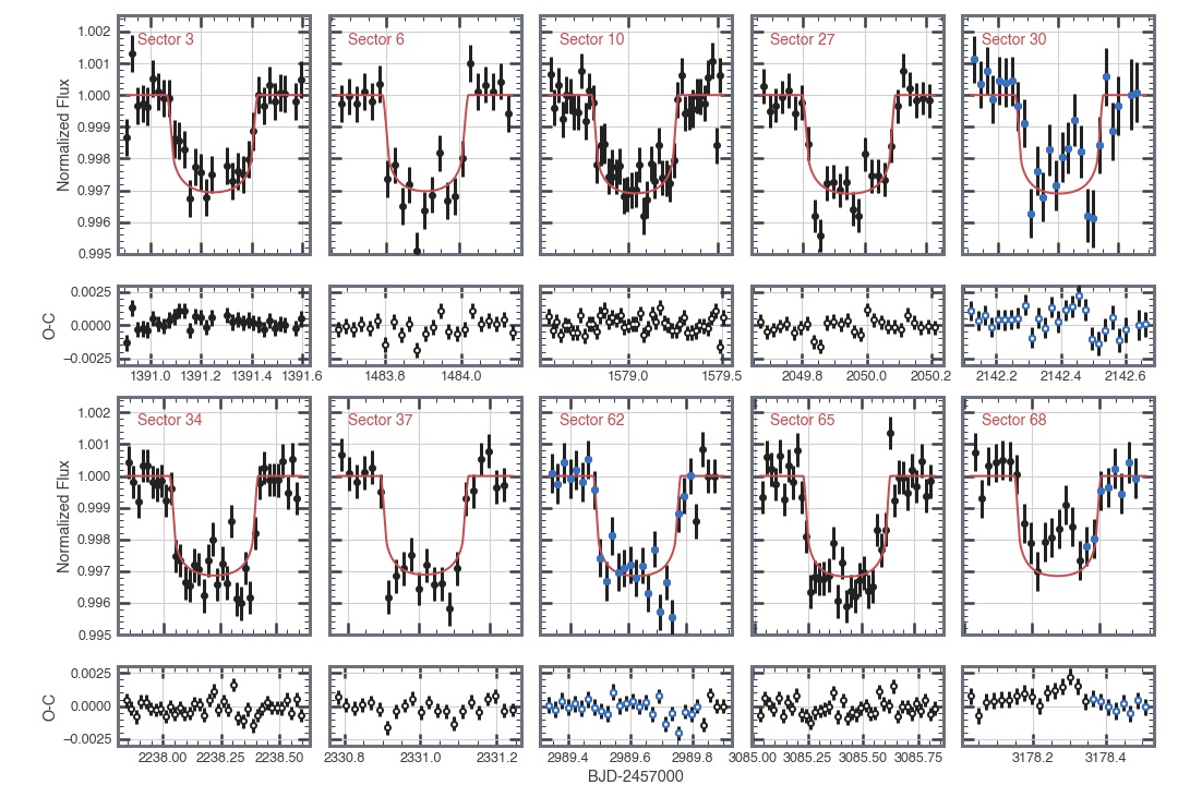
Ten primary transits of TOI-1338 b are observed during TESS’s observation (Sector 3, 6, 10, 27, 30, 34, 37, 62, 65, and 68). The light curve products are made of multiple cadences. We used 30-minute gsfc-eleanor-lite light curves for Sector 3 (Powell et al., 2022), 2-minute SPOC light curves for S6, 10, 62, 65, and 68, and 20-second SPOC light curves for S27, 30, 34, 37 (Jenkins et al., 2016).
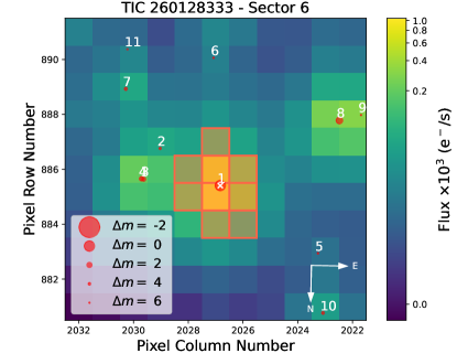
The two closest sources to TOI-1338 b have angular separations of 54.1” and 58.9”, both of them are fainter than TOI-1338 by 3 mags (Figure 1). None of them fall within the aperture of SPOC in the sectors when CBP transits occur. We also check the depth of the primary eclipses in the sectors of CBP transits from SPOC and GSFC light curves in S3, all of them showing consistent eclipse depth within 1.6%. The SOAR speckle imaging also indicates the absence of nearby sources within 3” (see Tokovinin et al. (2019) for a description of instrumentation). Therefore we conclude that the contamination of nearby sources should be minimal in both SPOC and GSFC light curves.
While most of the transits fall in the window of normal operation, the transit in Sector 30, 62, and 68 suffered from stray light of Earth and Moon (SPOC quality flag= 1E12). The stray light causes the background flux to rise and may cause uncertainties in the estimated background fluxes when performing aperture photometry and, thus introducing systematics in the produced light curves. As shown in Figure 2, the influence of stray light is most pronounced in Sector 30 and 68 light curves: large photometric jitters are present around the mid-transit and the post-transit portion of light curves. The transit in Sector 62 has a fall-off in fluxes near the egress phase. When binned to a 30-minute cadence, the egress/ingress of CBP transit is still well-resolved in Sector 62 and 68, but the egress is hardly resolved in Sector 30.
The variations in transit duration and midtimes are unique features for transiting CBP, and resolving the ingress/egress phase is crucial to precisely determining the magnitude of variations and measuring the movement and coordinates of different bodies. We decided to fit all the transits except for the one in Sector 30 due to its damaged egress phase. Later in Section 3.4 we will show the in-transit systematics will indeed affect the transit midtime determinations if we directly fit the light curves, but the bias is less severe if we fit the light curves globally using photodynamical modeling.
2.2 Detrending and Transit Times Fitting
We used the sap_flux product to measure the midtime and duration for each transit. The detrending and fitting are devised as follows. The light curves are first fitted with quadratic limb darkening transit model in batman (Kreidberg, 2015). The fitted parameters are transit midtime , planet period , semi-major axis scaled to stellar radius , impact parameter , planetary-to-stellar radii ratio , and two quadratic limb darkening coefficients (Kipping, 2013). We assume circular orbits during the midtime fitting. The likelihood function is used to measure the goodness-of-fit of the model compared to the observation. The model is first optimized using Monte Carlo Markov Chain (MCMC) for 30000 iterations. Once a best-fit model is found, the light curves are trimmed to shorter segments centered at the best-fit midtime, with lengths of two times of best-fit transit durations. The trimmed light curves are detrended with a linear slope, with in-transit data given zero weight during the linear fit. The flux errors are also rescaled to make the reduced . The scaling factors for transits in each sector are also listed in Table 1. Then the model is re-optimized using MCMC for another 30000 iterations. We also calculated the estimated transit duration from our fitted parameters via Equation 14111To the first order, we assume the binary-planet relative velocity is constant during the CBP transits, therefore the calculation of transit durations can be approximated to be similar to transits around the single-star system. However, the binary-planet relative velocity is constantly changing throughout the transits due to the lateral motion of binary, thus the transit profiles could be asymmetric in ingress/egress for circumbinary planets (see Figure 3 in Liu et al., 2013). A more precise transit duration estimate for transiting circumbinary planets would be derived from a photodynamical model. For TOI-1338 b, the asymmetry in transit ingress/egress is at most 15 minutes. in Winn (2010).
The measured transit midtimes and durations are listed in Table 1. Comparing the predicted transit mid-times of K20 and the observed mid-times, we found that while the observation in Sector 37 matches well with the prediction in K20, the rest of the observed transit midtimes deviates from K20 predictions by more than the magnitude of their predicted uncertainties, which is most evident in Sector 65 and 68 where deviations are readily comparable to the transit durations. The deviation between K20 predictions and TESS following observations could be caused by the imprecise system parameters, most likely the planetary orbital parameters, derived from the limited three transits observed in the TESS Primary Mission used in K20, and also could source from the gravitational interactions from the TOI-1338 c whose presence is unknown at that time. In Section 4.3 we will show that TOI-1338 c is indeed perturbing TOI-1338 b and contributes to the transit timing deviations we show here. Therefore we carry out photodynamical modeling to update the global parameters of TOI-1338 system in the next section.
| Sector | Transit Midtime | Duration | Error inflation factor | Predicted MidtimeaaPrediction from K20 |
|---|---|---|---|---|
| (BJD-2457000) | (hr) | |||
| 3 | 1391.2516 0.0073 | 8.5584 0.4226 | 0.7539 | - |
| 6 | 1483.9048 0.0029 | 5.9564 0.2135 | 1.0100 | - |
| 10 | 1579.0423 0.0052 | 11.5838 0.4883 | 1.0110 | - |
| 27 | 2049.9515 0.0034 | 7.1834 0.3704 | 1.0309 | 2049.6930 0.0196 |
| 30 | - | - | - | 2142.3991 0.0224 |
| 34 | 2238.2258 0.0034 | 9.5885 0.2923 | 1.0162 | 2237.9229 0.0236 |
| 37 | 2331.0148 0.0024 | 5.8707 0.1752 | 0.9953 | 2330.9984 0.0264 |
| 62 | 2989.6356 0.0047 | 7.6709 0.4334 | 0.9886 | 2989.3540 0.0509 |
| 65 | 3085.4243 0.0044 | 10.2463 0.3505 | 0.9953 | 3084.8165 0.0693 |
| 68 | 3178.2853 0.0077 | 6.2203 0.6371 | 0.9498 | 3177.9790 0.0600 |
3 Photodynamical Modeling
In this section, we present the photodynamical analysis of TOI-1338. We firstly describe our photodynamical model in Section 3.1 and the system parameter retrieval strategy in Section 3.3; we also discuss some potential bias by transit systematics in Section 3.4 and test the validity of photodynamical solutions in terms of the dynamical stability in Section 3.5.
3.1 Model Setup
The system parameters of circumbinary planet systems are often exhaustively explored by photodynamical modeling (e.g., Doyle et al. (2011b), Welsh et al. (2012)). Given initial orbital and mass parameters, the N-body integrator solves the equations of motions of binary and planets and produces in-time observables, i.e., eclipse, transit light curves, and radial velocity time series. The synthetic data are compared to the observations, and system parameter credible intervals are explored by sampling algorithms (e.g., MCMC) with related observational uncertainties.
The dynamical status of a two-planet circumbinary system can be characterized by 22 parameters, equivalent to six binary and twelve planetary osculating orbital elements (, and mean longitude ), and four masses (). The ascending node angle of the binary orbit can be further set to zero, which leaves 21 parameters. Synthetic stellar eclipse and planet transit light curves can be produced by the relative positions of each body, which require the stellar and planetary radii (), primary-to-secondary star surface brightness ratio in TESS band , and two sets of quadratic law limb darkening coefficients, for which we used the triangular sampling in Kipping (2013). In total 6 additional parameters are needed for light curve synthesis. The secondary eclipses show flat-bottom in-eclipse profiles and have low SNR, therefore the limb darkening coefficients of the secondary star are not well constrained and thus are set to be the same as the primary star222A more sensible treatment for the limb darkening coefficients of the secondary star would be using the theoretical values presented by Claret (2017): for K, =5.0, and [Fe/H]=0.0. Using these theoretical values, the maximum difference between the new secondary eclipse light curves and our adopted model is 10 ppm, only manifesting during the ingress/egress phase. The error is much smaller than the observational error of 200 ppm and thus this barely changes the overall likelihood of the photodynamical fitting and parameter sampling.. The dynamical modeling also issues radial velocity curves relative to the system barycenter. Thus, the system barycentric velocity is modeled as three instrument-dependent parameters for HARPS and ESPRESSO(pre-2019 and post-2019). In summary, 30 parameters are needed in photo-dynamical modeling in the case of the TOI-1338 system.
We outline our photodynamical model as follows. The system is initialized in the Jacobian coordinate, namely, the object is initialized in the order of its semi-major axis to the primary star. We use the IAS15 integrator in the python package rebound (Rein & Liu, 2012) to solve the motion of all objects. The integration is done in the center-of-mass coordinate. We use batman (Kreidberg, 2015) to generate synthetic light curves from the relative coordinates of different bodies on the sky-projected plane centered on the system barycenter, after linear corrections for the light travel effect. The radial velocity data precision of ESPRESSO achieved 1 m/s, calling the need for relativistic correction, therefore the simulated RVs are further corrected with light travel effects, transverse Doppler, and gravitational reddening effects (Zucker & Alexander, 2009; Konacki et al., 2010; Sybilski et al., 2013). However, later we found that these will not significantly alter the fitted result as the RV variations are absorbed into the barycenter velocity. Tidal effects are not included since it suffered from uncertainty in tidal parameters and is estimated to have an amplitude m/s, which is much lower than the total amplitude of relativistic effects ( m/s).
For the case of the TOI-1338 system, the General Relativity (GR)-induced apsidal precession is around 9.01 arcsec per year. The apsidal precession rate induced by tides is times smaller than the GR term, following the prescription in Correia et al. (2013). We do not include the GR and tidal effects in our dynamical model.
The reference epoch is fixed at BJD=2458300.00, approximately 90 days before the first observed CBP transit in Sector 3. Using the best-fit values in K20, we integrate the TOI-1338 system into our reference epoch and record the result as an initial guess of the model parameters. The orbital parameters of the outer planet are derived from S23, with randomly generated node angles and inclinations but satisfying the system stability limit (mutual inclination smaller than 40∘, see Supplement Figure 8 of S23).
We adopt the differential evolution Monte Carlo Markov Chain (DE-MCMC, Ter Braak, 2006) in emcee to sample the parameter space. The range of parameters is displayed in Table 2. Flat priors are assumed for all parameters. The function is used to define the goodness-of-fit of the model. This is computed by the square of the differences between observation and synthetic photometric/RV data, divided by the square of observational errors.
3.2 Fitted Data
Using the photodynamical model described in the above section, we simultaneously fitted the binary eclipse light curves, transits of TOI-1338 b in TESS light curves, and the radial velocity data published in S23.
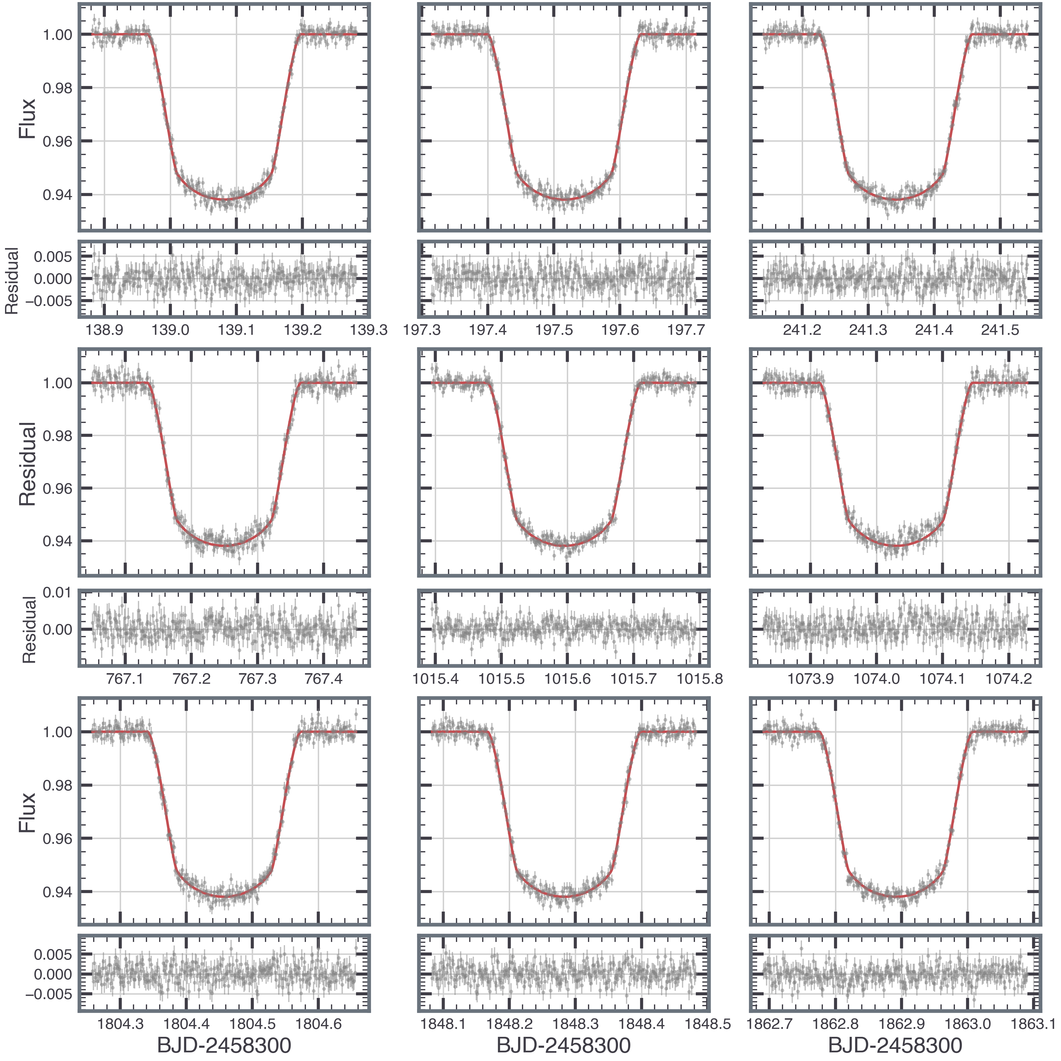
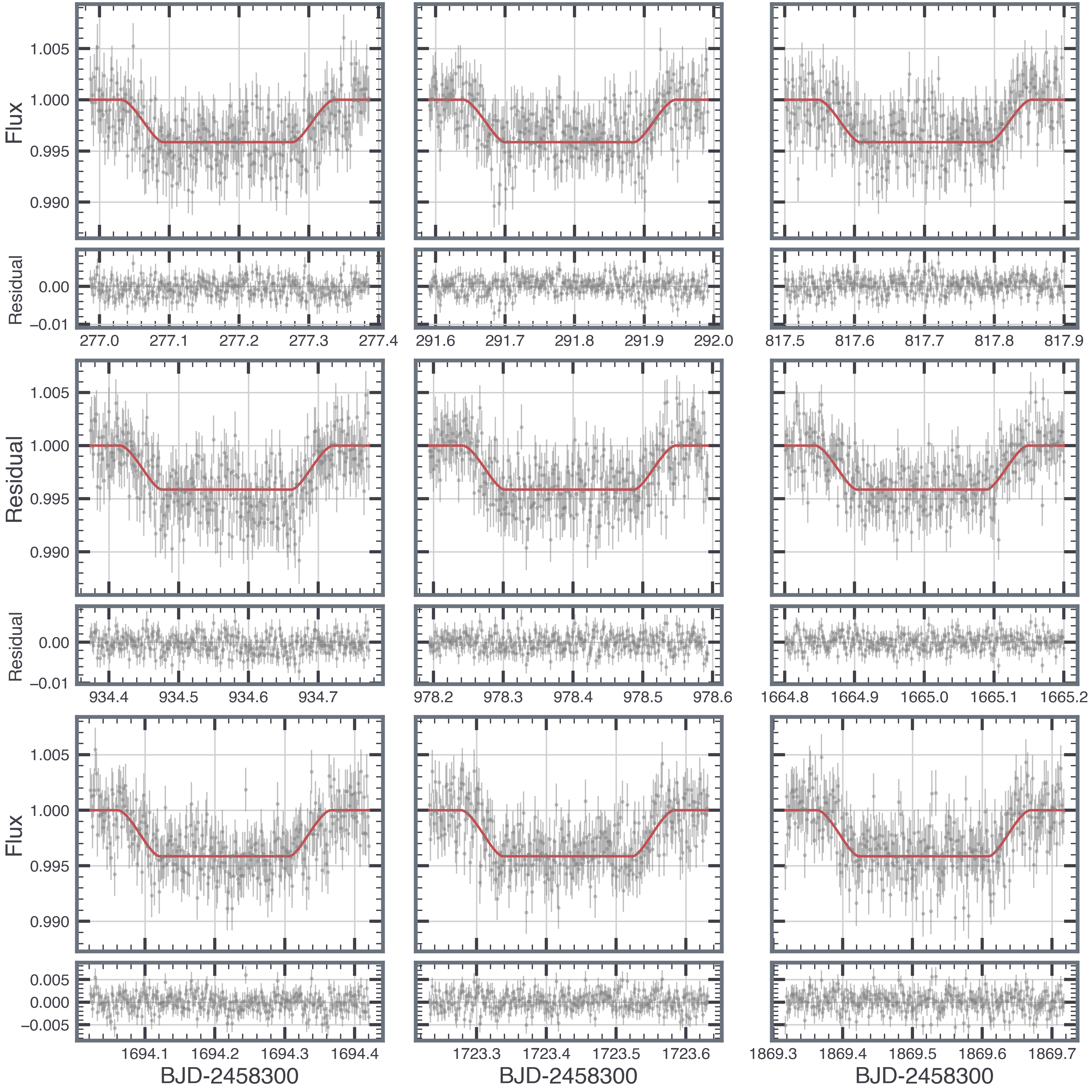
We fitted nine TOI-1338 b’s primary transit events, excluding one transit event in Sector 30 since it is severely affected by systematics. To speed up the integration speed and prevent the potential bias delivered by the instrumental systematics or out-of-eclipse trend (Orosz et al., 2019), we select nine primary and secondary eclipses, respectively, for the following photodynamical modeling, based on the ranking of their reduced . Figure 12 and 13 in Appendix B show the selected nine primary eclipses and secondary eclipses. The transit and eclipse data are detrended according to Section 2.2. Once an initial dynamical result that can reproduce the observed light curves is obtained, the light curves are detrended again with the more precise transit/eclipse midtimes and durations inferred from the dynamical result.
61 HARPS and 123 ESPRESSO RV data points are published by S23. Many of these RV data have been flagged to be potential FWHM/bisector outliers, or due to the data being taken at the time of binary or planetary transits. We exclude RV data with outlier flags for our photodynamical model, leaving 58 HARPS and 103 ESPRESSO RV data to be modeled.
3.3 Planetary System Parameters Sampling
We first perform a joint fit to the stellar eclipse, transit photometry, and HARPS/ESPRESSO radial velocity data. At the starting stage, 100 chains evolved from the initial guess with small offsets to explore the parameter space. After the chains remained stable in small ranges, we evolved 100 chains for another 690000 steps. We remove the first 350000 steps as the burn-in phase. The rest of the 340000 steps from 100 chains are concatenated together, and they are sampled every 1000 steps to make the posterior sample with a total size of 34000. The Gelman-Rubin statistics of all parameters are smaller than 1.05 (Brooks & Gelman, 1998). The autocorrelation steps of fitted parameters vary between 1972 and 5213, giving at least 6522 effectively independent samples in total. The median and uncertainties (defined as the 16th and 84th percentiles of the posterior distribution) of each fitted parameter are listed in Table 2.
We examined the residuals of all eclipse, transit, and RV residuals and found the best-fit solution from joint fit provides a good match to the light curve data. However, we found a very significant periodicity corresponding to the binary period in HARPS RV residuals (FAP 0.1%) but none in ESPRESSO residuals. In other words, there is inconsistency in the binary RV motion between HARPS and ESPRESSO RV data. The peak-to-peak amplitude of HARPS residual is m/s, and peaks around when the binary is in its conjunction. This is not likely a problem associated with our photodynamical code as this inconsistency persists when we perform a joint RV-only Keplerian fit analysis (see details in Appendix A).
To circumvent the potential bias on the binary orbital parameters brought by RV inconsistency, we experimented with two additional photodynamical fits performed individually to ESPRESSO and HARPS data (and hereafter we refer to these two experiments as esp-only and harps-only analyses), with the light curve dataset identical to the joint fit. We took 100 samples from the joint fit posterior samples and evolved them for 300000 steps. We trimmed the first 150000 steps as the burn-in phase, and the Gelman-Rubin statistics for the remaining chains are smaller than 1.04 for all parameters. The effective sample sizes are at least 4263 and 3624 for esp-only and harps-only posteriors, respectively. We kept the last 150000 steps and sampled every 1000 steps to make the posterior distributions. The median and uncertainties of fitted parameters from the esp-only and harps-only analysis are presented in the second and third columns of Table 2.
Most parameters from esp-only and harps-only fit are 1-2 deviant from joint analysis, while some of them show 3 discrepancy. For the binary orbital parameters, the joint fit and esp-only fit show close agreement, while the binary eccentricity from harps-only fit is around 3- larger than those from the other two analyses, which probably stems from the RV inconsistency from HARPS data. The binary mass ratio and orbital parameters of TOI-1338 b inferred from the three analyses are different too, with joint and esp-only analysis having 3 discrepancy on binary mass ratio and that from harps-only being intermediate between the former two. We provide some intuitions of the potential causes. TOI-1338 is a single-line binary, so only the mass function (related to the mass ratio, absolute mass, and binary period, eccentricity, inclination) can be constrained from RV data. The degeneracy between the mass ratio and the mass function is solved by accounting for the exact timing of planetary transit. For example, the peak-to-peak amplitude of transit timing variations nonlinearity of CBP transit is, in the first order, related to the binary phase and the exact projected stellar location, which is further related to the semi-major axis of the transited star and hence the mass ratio can be constrained (Schwamb et al., 2013; Armstrong et al., 2013; Kostov et al., 2013, 2014). The CBP transit durations also depend on the relative velocity difference between the binary star and planet. For the latter one, the velocity of the planet is also related to the total masses of the inner binary, and thus can also contribute to solving the mass ratio from the mass function. This degeneracy is also supported by the clear correlation between the mass ratio and the inner planetary orbit parameters (, , eccentricity vectors). Following this thread of thought, we attributed the discrepancy of mass ratio derived from the two analyses to the difference in planetary orbit solutions, since we found the derived mass function from joint and esp-only analysis is consistent within 1.
Despite the difference in inner planetary orbit solutions, the best-fit of the transit light curve between joint and esp-only analysis has a negligible difference, which is and for 10183 cadences, respectively. But given the inconsistency between HARPS and ESPRESSO data, we prefer esp-only solution over the joint-fit one. Between esp-only and harps-only solutions, the in transit is almost identical, and the harps-only solution is only marginally preferred over the esp-only ones in terms of the . However, we think the outer planet’s orbit is better constrained by the ESPRESSO data, for its higher precision and more observations.
At the writing of the manuscript, Sebastian et al. (2024) published the absolute dynamical masses of TOI-1338 AB for M⊙ and M⊙, respectively. This measurement is more aligned with our esp-only solution. Additionally, in Section 3.5 we will show that the esp-only solution are more dynamically stable compared to the other two sets of solutions. Therefore, among the three analyses presented in this section, we adopt the solution of esp-only analysis.
In our nominal photodynamical model, we assume constant zero flux dilution for all TESS sectors. For completeness of the photodynamical discussion, we also run a model accounting for different dilution levels in different sectors. Applying a unique dilution factor to each sector is necessary for missions like TESS since the star’s location in the CCD plane in each sector is different and so is the amount of flux from the nearby stars expected to contain within the target’s aperture. In this simulation, we include the primary and secondary eclipse light curves in the same nine sectors as the transits were observed to help better constrain the dilution factor. The dilution factors are allowed for negative values to reflect the situation where the background fluxes are potentially over-substracted. However, we found the dilution factor of each sector is consistent with zero within 1, and the important parameters like stellar mass ratios did not change significantly. We attribute this to nearly consistent or negligible dilution within TOI-1338 in different sectors and proceed with the remaining discussion with the model without dilution consideration.
| Paramter | Unit | Prior Range | TESS+ESP+HARPS | TESS+ESP (adopted) | TES+HARPS |
|---|---|---|---|---|---|
| Binary | |||||
| M⊙ | [0.8,1.3] | ||||
| - | [0.26,0.34] | ||||
| R⊙ | [1.0,1.5] | ||||
| R⊙ | [0.2,0.4] | ||||
| day | [14.6,14.7] | ||||
| - | [0.15,0.16] | ||||
| deg | [89,92] | ||||
| deg | [80,150] | ||||
| deg | [225,310] | ||||
| - | [0.99,1.0] | ||||
| - | [0,1] | ||||
| - | [0,1] | ||||
| Planet b | |||||
| day | [94.5,96.5] | ||||
| deg | [89.0,91.5] | ||||
| deg | [80,140] | ||||
| deg | [-0.5,0.5] | ||||
| RJup | [0.5,0.8] | ||||
| - | [-0.5,0.5] | ||||
| - | [-0.5,0.5] | ||||
| MJup | [0.0,0.1] | ||||
| Planet c | |||||
| day | [200,235] | ||||
| deg | [50,130] | ||||
| deg | [0,360] | ||||
| deg | [-50,50] | ||||
| - | [-0.55,0.55] | ||||
| - | [-0.55,0.55] | ||||
| MJup | [0.0,0.6] | ||||
| Instrument Parameters | |||||
| km/s | [30.5,31.0] | - | |||
| km/s | [30.5,31.0] | - | |||
| km/s | [30.5,31.0] | - | |||
| Derived Parameters | |||||
| M⊙ | - | ||||
| M⊕ | - | ||||
| M⊕ | - | ||||
| R⊕ | - | ||||
| deg | - | ||||
| deg | - | (,95%) | |||
| deg | - | ||||
| deg | - | ||||
| deg | - | ||||
| deg | - | ||||
| Best-fit | |||||
| 15768.7 | 15650.7 | 15386.7 | |||
| 10164.7 | 10166.86 | 10164.4 | |||
| 5166.36 | 5169.92 | 5164.72 | |||
| 437.82 | 304.96 | 58.06 |
Note. — Osculating jacobian orbital parameters valid at BJD=2458300.0
3.4 The Effect of In-Transit Noise
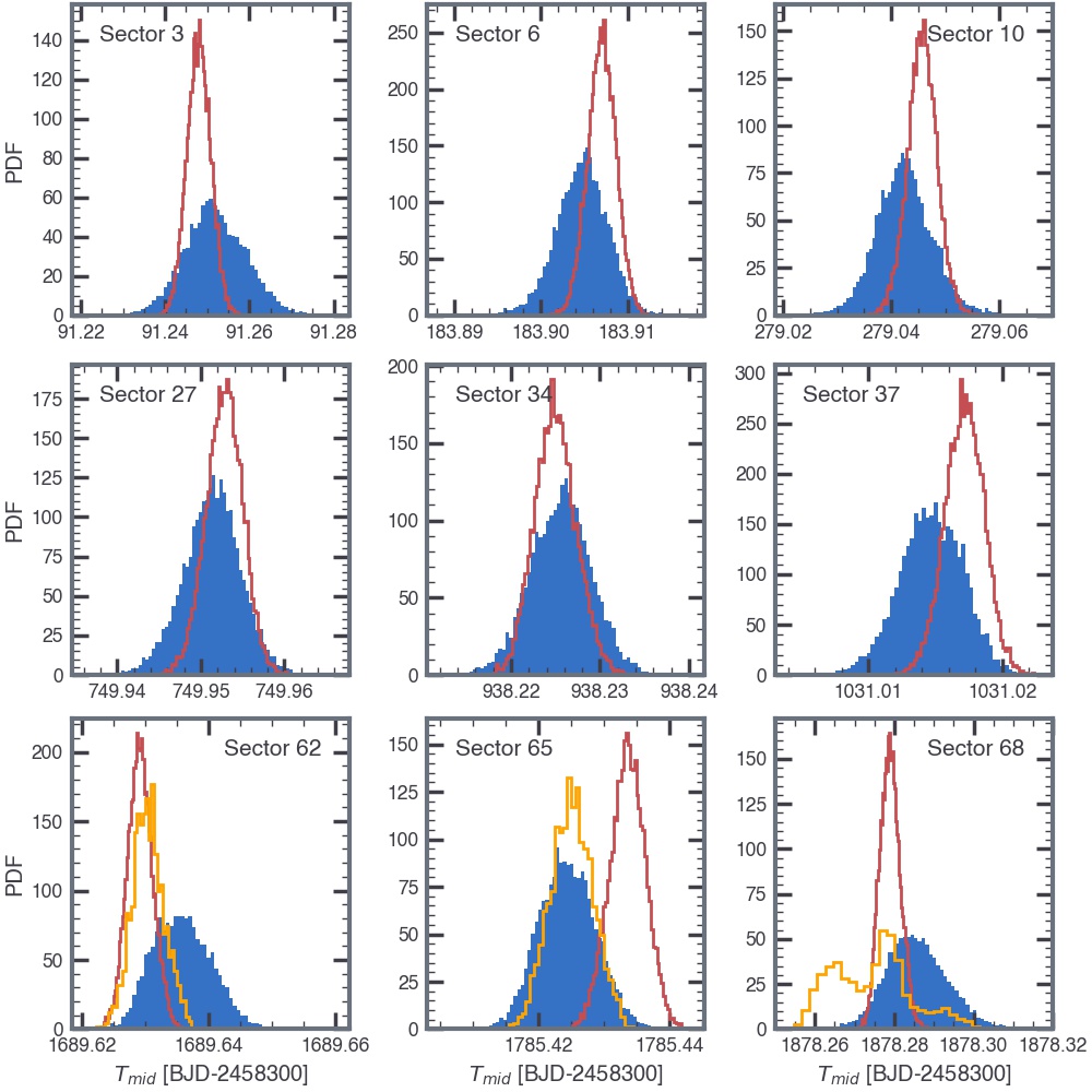
In Figure 3, we compare the posteriors of transit midtimes of all sectors from the direct fitting (Table 1) and photodynamical fitting. Generally, the uncertainties of transit midtime from the global photodynamical model are smaller than those from direct fitting, and the midtime posteriors from two analyses are consistent within 1, except for the transits in S62, S65, and S68. The in-transit systematics that cannot be removed from the detrending technique described above could potentially bias the midtime estimates and thus the photodynamical modeling. To investigate whether the in-transit systematics, especially in S62 and S68, have a significant effect on the photodynamical modeling, we took an independent analysis of midtime fitting incorporating the Gaussian process (GP) to see if the systematic-corrected midtimes are consistent with the results from the photodynamical model. The GP could model the noise and transit altogether to yield more unbiased midtime results compared to the direct fitting. This is done by using the python package juliet (Espinoza et al., 2019).
We show the GP-correct midtime posteriors in S62, S65 and S68 in Figure 3. For the S62 and S68, the midtimes derived from the photodynamical modeling are more discrepant with those from direct fitting but are more consistent with the results of GP-corrected midtimes. This indicates that our midtime posteriors from the global photodynamical modeling do not greatly suffer from the systematics in S62 and S68 as the direct fitting does. However, the transit in Sector 65 displays difference between photodynamical modeling and other results. We postulate that this is caused by the very sharp flux jump near the egress phase of this transit event (see Figure 2), which could not be sufficiently modeled by the GP. This could potentially make the predicted egress time from the direct fitting end earlier and thus the midtime will be a little earlier too.
3.5 Stability Analysis
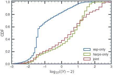
To investigate the stability of the posterior solutions from our photodynamical modeling, we calculated a dynamical Mean Exponential Growth factor of Nearby Orbits (MEGNO; Goździewski et al., 2001; Cincotta et al., 2003) for all three sets of solutions in Table 2. MEGNO is a numerical tool to differentiate chaotic and stable motion. Specifically, if the orbits are stable, the final will converge to 2, else it will increase as time. We integrate each solution with the whfast (Rein & Tamayo, 2015) integrator for 50 kyr and calculate the MEGNO value of the system. The cumulative density function of calculated for three sets of solutions are shown in Figure 4. The median value of joint-, esp-, and harps-only solutions are 6.13, 1.98, and 7.84, respectively. This result suggests the majority of posterior solutions ( for ) from esp-only analysis is stable within 50 kyr, while the other two sets of posteriors are more likely to become unstable within the integrated time. Examining the unstable solutions with shows that the larger the eccentricity of TOI-1338 c is, the more likely the system would get unstable. Note that the joint and harps-only solutions yielded for while esp-only solutions have . This is also consistent with the conclusion of S23 that the eccentricities of both planets should be lower than 0.1 to keep the system stable. Based on the results from the stability analysis, it is advised to take the esp-only solutions as the final adopted solutions from our photodynamical modeling.
4 Results
In our photo-dynamical modeling, we analyze the mass constraint of TOI-1338 b, which could potentially have an extremely low density as g/cm-3, in Section 4.2. We also discuss the mutual inclination of non-transiting planet TOI-1338 c relative to the binary plane in Section 4.3. Then we present the future primary transits forecast in Section 4.4.
4.1 Eclipse Timing Variation Analysis
The mass of the circumbinary planet is traditionally constrained by the eclipse timing variations (e.g., Doyle et al., 2011a; Welsh et al., 2012). The planet will gravitationally perturb the binary and cause the apsidal precession of binary orbits, which would appear as a divergence of the binary period derived from primary and secondary eclipses if the binary orbit is eccentric. Futhermore, if the planet is non-coplanar with the binary, the inclination of binary orbit would also go through precession and manifest as the eclipse depth variations, though this would work most effectively for grazing eclipses (see, e.g., Socia et al., 2020; Goldberg et al., 2023). The planet’s mass could also be constrained by the short-term “choppings” in the Observation minus Computed (O-C) diagram, the time-scale of which is comparable to planetary orbit (Rappaport et al., 2013).
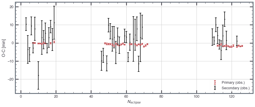
In the best-fit model excluding GR, the total apsidal precession of binary orbit is 31.35 arcsec per year. The precession rate caused by planet b is 14.56 arcsec per year, slightly larger than the expected GR-induced precession rate ( arcsec per year) and is around 10 times higher than the tidal-induced precession rate, but is smaller than the precession rate induced by the outer planet ( arcsec per year). In the 5-year TESS’s observation baseline, this precession rate will lead to a divergence of 0.8 minutes between primary and secondary eclipses when they are fitted to common ephemerides. However, this divergence amplitude is not readily observable because it is much smaller than the typical uncertainty of the secondary eclipse midtimes (5-6 min), as seen from Figure 5. The short time-scale oscillations of O-C curves have an amplitude of 0.03 min, dominated by the outer-planet perturbation. We also tried out a few cases when TOI-1338 c is misaligned by mutual inclination up to 40∘, and the amplitude of primary ETVs is still smaller than the typical uncertainties of 0.3 min. Therefore the ETVs are not likely to constrain the mass of TOI-1338 b nor the inclination of TOI-1338 c.
4.2 The Mass of TOI-1338 b
Our adopted photodynamical solutions in Table 2 show that the mass of TOI-1338 b is . To determine the source of the inner planetary mass constraint, we run two additional groups of modeling with modified fitted data to see whether the mass of TOI-1338 b is constrained or not. The first group of modeling fits the stellar eclipse photometry in the first year of TESS observation (S3-S10) and the full set of RV observations, this choice aligns with K20 and removes the possible mass constraints delivered by long-term ETVs. However, the mass constraints for planet b remain the same as the adopted solutions. The second group of modeling fits all TESS photometry but without RV data, with the mass of the binary and outer planet fixed at the best-fit value of the adopted solution. In this case, the mass distribution of the TOI-1338 b is highly skewed to zero, with a 95% upper limit of . Therefore we conclude that the mass reported in Table 2 are constrained from the RV data.
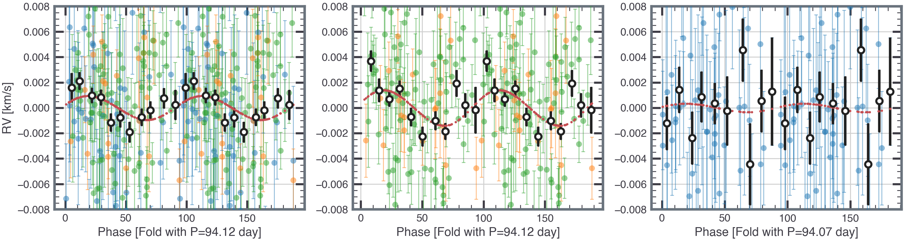
We then look for the RV signal of TOI-1338 b in the current RV dataset. This is done by subtracting the observed RVs from the secondary star and outer planet’s RV signal simulated issued from the integrator, the parameters of which are taken from the best-fit solutions. The residuals should correspond to the RV signal of TOI-1338 b. The phase-folded residuals are shown in Figure 6. In the left and middle panel of Figure 6, corresponding to the best-fit TOI-1338 b’s RV signal from the joint and esp-only analyses, we observe clear modulation in observed RV residuals folded at the period of TOI-1338 b, with a semi-amplitude of and 1.5 m/s, respectively. To assess the compatibility of this modulation with our model, we have included in Figure 6 the predicted RV signals of TOI-1338 b from the best-fit model at each of the RV observation epochs, represented as red points. The figure demonstrates a close match between the predicted signals and the observed modulations. It is important to note that some deviations of the observed RV signals from the model predictions are apparent, particularly in certain phase bins. These deviations may be attributed to the uneven coverage of RV observations over the planet phases, especially in esp-only results where the current RV data are sparser in the latter half of the planetary period (phase day).
The harps-only solution provides a mass constraint of TOI-1338 b consistent with zero. As is also seen in the right panel of Figure 6, there is no apparent signal when the RVs from the secondary star and TOI-1338 c are subtracted. After subtracting the best-fit signal of TOI-1338 b, the changed from 57 to 58, so there is no improvement made. It is likely that the RV signal of TOI-1338 b is completely submerged in the noise of HARPS RV measurements. Also note that in Section 3.3 we report inconsistency in binary RV signal between HARPS and ESPRESSO with amplitude m/s. Such large systematics could be detrimental to the search of planets with signals as weak as only 1 m/s.
The study of S23 and K20 have both formerly provided mass constraints on TOI-1338 b. S23 uses RV datasets identical to ours and perform Keplerian fit to the RV and find tentative signals at periodicity around 100 days consistent with TOI-1338 b, though the significance of this signal is not high enough and thus they report a 99% upper limit of for TOI-1338 b. Note that their analysis is purely based on RV data, independent of any prior knowledge of orbital parameters TOI-1338 b, including the orbital phases which could be precisely informed by the transit events. K20 derived for the planet by photodynamical modeling of 1.5 yr TESS photometry and CORALIE/HARPS RV measurements. The mass constraint mainly comes from the seven HARPS RV measurements obtained at that time. Our method is more similar to the analysis of K20, except that we incorporate more RV measurements from ESPRESSO with higher precision and yield more precise mass constraints.
4.3 The Inclination of TOI-1338 c
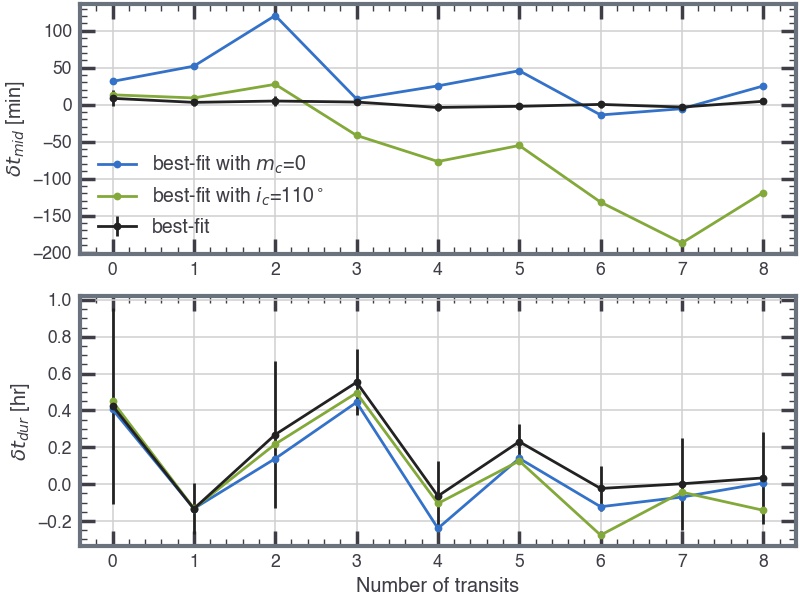
In Figure 7, we show evidence that the TOI-1338 b is gravitationally perturbed by TOI-1338 c, which manifests as TTVs and TDVs in models where we fixed the mass of TOI-1338 c as zero. The variations in transit timing are more prominent, in several transit events the deviations can be detected with several , whereas the variations in transit durations are close to the measured uncertainties. Moreover, the inclination of the outer planet’s orbit also changes the TTVs, which may allow us to put meaningful three-dimensional constraints on the outer planet’s orbit, which is inaccessible to the RV method by which TOI-1338 c is discovered.
The mutual inclination between the binary and outer TOI-1338 c can be calculated via
| (1) |
The three analyses yielded a mutual inclination of TOI-1338 c around 10∘ relative to the binary orbital plane, consistent with a coplanar configuration. However, our adopted model prefers a non-transit nature of TOI-1338 c, even though we did not impose any criterion on it.
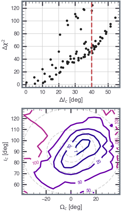
To explore how sensitively the data constrain the mutual inclination of TOI-1338 c , we run a suite of additional fits, with being between 50∘ and 130∘ and ranging between -40∘ and 40∘ and a step of 5∘. All other parameters are fixed at the best-fit value of joint analyses in Table 2, except that , , , , , , , and are further optimized by DE-MCMC. The inclination and node angle of the inner planet are not sensitive to the transit timing and are therefore kept fixed. These parameters are optimized against the observational dataset identical to the adopted solutions, except that binary eclipse light curves are excluded since the ETVs are not sensitive to the inclination of TOI-1338 c (See Section 4.1) The model optimization is carried out by DE-MCMC, with 40 chains for each experiment, and run for 4000-21000 steps (usually when the outer orbit is kept at high , the optimization will need to run longer chains). Optimization ends when we visually confirm that the remains constant for more than 50% of the steps.
The optimized map of the dynamical fitting is shown at the bottom of Figure 8. We find the minimum exists in (, )=(95∘, 10∘), consistent with the solutions provided in Table 2. That is, a lower mutual inclination of TOI-1338 c is favored by the current data, and the fits become worse in larger mutual inclinations, as shown in the top panel of Figure 8. When examining the of transit light curves and RV data separately, we found that when TOI-1338 c is fixed at high the optimized results could provide a good match to the observed transit midtimes and durations, while the fits of RV data become worse.
However, compared to the nominal photodynamical models in Section 3, only the eclipse photometry is removed in the models in this section, therefore the degree of freedom of these model optimizations is still as high as 10336. At higher , the is only 35-40, which may not be a statistically significant argument against high if seen from the perspective of reduced-. Therefore, based on the current data, lower mutual inclination between binary and outer planet’s orbit is marginally favored over high mutual inclination scenarios.
4.4 Future Transits Forecast
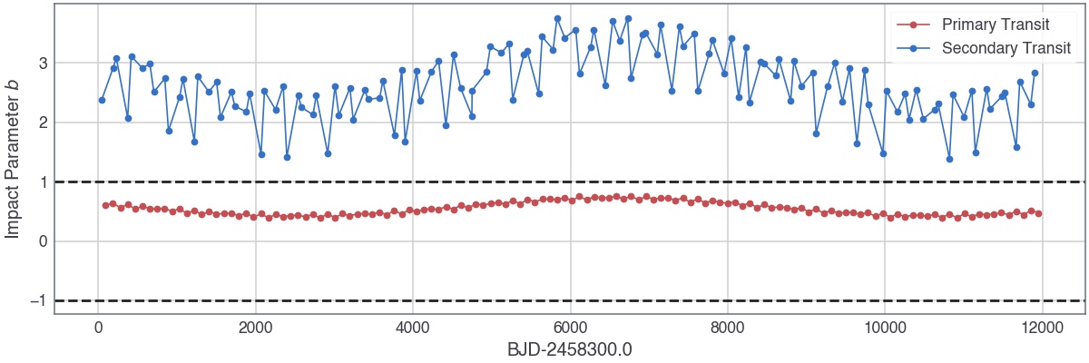
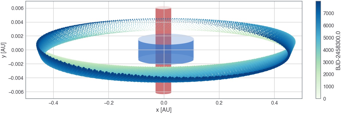
We present the future primary transit of TOI-1338 b in Table 3. It shows that TOI-1338 b will permanently transit the primary star, which is similar to Kepler-47 b (Orosz et al., 2019). This is partly due to the coplanarity of the orbit of TOI-1338 b relative to the binary planet () and the sufficiently large primary radius. Integrating the best-fit model with rebound, in Figure 9 we present the impact parameter of TOI-1338 b in each conjunction with the primary and the secondary star. Due to perturbation of the inner binary, the orbital plane of TOI-1338 b will undergo precession and the inclination of TOI-1338 b will follow sinusoidal-like variations.
Our best-fit models suggest that no secondary transit occurs in the current TESS observation. Following Martin & Triaud (2015), the minimum mutual inclination of TOI-1338 b ever transiting secondary star is 0.277∘, whereas our posterior samples yielded a . This partly explains why secondary transits of TOI-1338 b are rare in our posterior models. The orbit of TOI-1338 b will hardly precess into an orientation that the planetary and secondary star’s orbits are mutually intersected.
With a TESS mag of 11.45 mag and a period of 95 days, TOI-1338 b is an ideal circumbinary planet target for JWST transmission observation. TESS is scheduled to re-observed TOI-1338 in Year 7 observation, and another three primary transits of TOI-1338 b are expected to occur in the observing window of Sector 89, 93, and 96 between 2025 Match and September. We encourage more follow-up observations to be carried out to TOI-1338 b transits to update and refine future transit ephemerides.
5 Dicussion and Conclusion

In this work, we perform a system update of the TOI-1338 with two circumbinary planets. Combined with the latest TESS light curves and published radial velocity data, we carry out photodynamical analysis to self-consistently account for the mutual interactions between bodies within the systems.
We determined a coplanar configuration for TOI-1338 c relative to the binary plane , with a 99% upper limit of . Therefore the genuine mass of TOI-1338 c is determined to be M⊕. This constraint mainly comes from the additional number of observed transits of TOI-1338 b and the precise RV measurements, where the gravitational pull from the outer planet starts to manifest in the transit timing variations of the inner planet (see Figure 8). Together with the spin-orbit alignment between the primary star and the orbit of TOI-1338 b (projected spin-orbit angle of ) (Hodzic et al., 2020), the whole system is in an alignment between primary’s spin axis and binary-planet orbit configuration. This suggests the whole system forms from a single disk with no breaking or warps.
With our refined mass ( M⊕) and radius ( R⊕) for TOI-1338 b, we derived a low bulk density of g/cm-3. This is comparable to circumbinary planet Kepler-47 c which also has a low bulk density of 0.17 g/cm-3. In Figure 10 we show TOI-1338 b and other low-mass sub-Saturns in the mass-radius diagram, with the tide-free thermal evolution models for sub-Saturns from Millholland et al. (2020) at TOI-1338 b’s age (4 Gyr, K20) and insolation. We estimate the envelope mass fraction, fenv, to exceed 50%, implying that TOI-1338 b possesses a substantial envelope, akin to several super-puffs found around single stars (e.g., Kepler-79 d with f, Millholland et al. (2020); K2-24 c with f, Petigura et al. (2018)). Lee & Chiang (2016) suggests planets with such low density might have migrated from a distant region where the disk is cool and has low opacity, enabling efficient cooling of the accretion and forming a massive envelope even with a low-mass core. This hypothesis aligns with the general picture that most observed CBPs may have undergone migration during their formation process (e.g., Pierens & Nelson, 2013; Coleman et al., 2023a, b), due to the local low growth rate of planetary cores near the stability limit, which hinders the in situ formation of CBPs (Pierens et al., 2020, 2021).
With a TESS-band magnitude of 11.45 and a J-band magnitude of 10.95, TOI-1338 is an optimal target for future follow-up and transmission observation. Taking an average equilibrium temperature of 495 K for TOI-1338 b, we calculated the transmission spectroscopy metric of TOI-1338 b to be 8617, which is slightly below the recommended threshold of 96 for sub-Jovian planets (Kempton et al., 2018). Although previous measurements show featureless transmission spectra for low-density sub-Saturns (Libby-Roberts et al., 2020; Chachan et al., 2020), hypothetically owing to the high altitude hazes or circumstellar rings (Wang & Dai, 2019; Gao & Zhang, 2020; Ohno & Fortney, 2022), it would still be crucial to test this scenario in the infrared band to see if the hazes or rings are genuinely present and inflate the apparent radius of the planet.
We provided an updated future primary transit ephemerides of TOI-1338 b in Table 3. In our posterior models, TOI-1338 b will permanently transit the primary star at all nodal precession phases, owing to the extreme coplanarity with the binary plane and the large radius of the primary star. We encourage more follow-up observations of TOI-1338 b’s primary transit to refine the system parameters.
| Transit Midtime | Year | UTC | Duration | Impact Parameter |
|---|---|---|---|---|
| (BJD—2,455,000) | (hour) | |||
| 2024-02-26 | 14:14:38.8 | |||
| 2024-05-30 | 07:58:48.0 | |||
| 2024-09-02 | 08:42:39.7 | |||
| 2024-12-04 | 02:43:02.5 | |||
| 2025-03-09 | 22:52:56.4 | |||
| 2025-06-10 | 10:04:01.9 | |||
| 2025-09-14 | 05:34:19.7 | |||
| 2025-12-16 | 02:13:28.3 | |||
| 2026-03-21 | 02:46:09.6 | |||
| 2026-06-22 | 21:32:23.9 | |||
| 2026-09-24 | 15:01:15.1 | |||
| 2026-12-28 | 15:17:48.8 | |||
| 2027-03-31 | 08:14:46.3 | |||
| 2027-07-05 | 04:34:41.4 | |||
| 2027-10-05 | 15:26:36.1 | |||
| 2028-01-09 | 10:35:34.8 | |||
| 2028-04-11 | 07:54:09.5 | |||
| 2028-07-15 | 06:21:08.1 | |||
| 2028-10-17 | 02:08:04.3 | |||
| 2029-01-18 | 15:24:22.0 | |||
| 2029-04-23 | 18:30:58.1 | |||
| 2029-07-25 | 08:24:41.9 | |||
| 2029-10-29 | 05:53:12.8 | |||
| 2030-01-29 | 16:56:13.1 | |||
| 2030-05-05 | 09:20:03.2 | |||
| 2030-08-06 | 09:01:46.7 | |||
| 2030-11-08 | 23:40:30.5 |
Acknowledgments
We thank the referee, Hans J. Deeg, whose comments greatly improved the quality and clarity of the manuscript. We also thank Fei Dai, Xian-Yu Wang, Sharon X. Wang, and Yuan-Zhe Dai for their helpful discussions. This work is supported by the National Natural Science Foundation of China (grant Nos. 11973028, 11933001, 1803012, 12150009) and the National Key R&D Program of China (2019YFA0706601). We also acknowledge the science research grants from the China Manned Space Project with No. CMSCSST-2021-B12 and CMS-CSST-2021-B09, as well as the Civil Aerospace Technology Research Project (D050105).
This paper includes data collected with the TESS mission, obtained from the MAST data archive at the Space Telescope Science Institute (STScI). Funding for the TESS mission is provided by the NASA Explorer Program. STScI is operated by the Association of Universities for Research in Astronomy, Inc., under NASA contract NAS 5-26555. The TESS data presented in this paper were obtained from the Mikulski Archive for Space Telescopes (MAST) at the Space Telescope Science Institute. The TESS light curves used in this work can be accessed via MAST (Team, 2021). The GSFC TESS light curves can be accessed in Powell, Brian (2022).
References
- Aller et al. (2020) Aller, A., Lillo-Box, J., Jones, D., Miranda, L. F., & Barceló Forteza, S. 2020, A&A, 635, A128, doi: 10.1051/0004-6361/201937118
- Almenara et al. (2022) Almenara, J. M., Hébrard, G., Díaz, R. F., et al. 2022, Astronomy and Astrophysics, 663, doi: 10.1051/0004-6361/202142964
- Armstrong et al. (2013) Armstrong, D., Martin, D. V., Brown, G., et al. 2013, Monthly Notices of the Royal Astronomical Society, 434, 3047, doi: 10.1093/mnras/stt1226
- Armstrong et al. (2014) Armstrong, D. J., Osborn, H. P., Brown, D. J., et al. 2014, Monthly Notices of the Royal Astronomical Society, 444, 1873, doi: 10.1093/mnras/stu1570
- Brooks & Gelman (1998) Brooks, S. P., & Gelman, A. 1998, Journal of Computational and Graphical Statistics, 7, 434, doi: 10.1080/10618600.1998.10474787
- Chachan et al. (2020) Chachan, Y., Jontof-Hutter, D., Knutson, H. A., et al. 2020, The Astronomical Journal, 160, 201, doi: 10.3847/1538-3881/abb23a
- Chen & Kipping (2021) Chen, Z., & Kipping, D. 2021, 12, 1. https://arxiv.org/abs/2112.00966
- Cincotta et al. (2003) Cincotta, P. M., Giordano, C. M., & Simó, C. 2003, Physica D: Nonlinear Phenomena, 182, 151, doi: 10.1016/S0167-2789(03)00103-9
- Claret (2017) Claret, A. 2017, A&A, 600, A30, doi: 10.1051/0004-6361/201629705
- Coleman et al. (2023a) Coleman, G. A., Nelson, R. P., & Triaud, A. H. 2023a, Monthly Notices of the Royal Astronomical Society, 522, 4352, doi: 10.1093/mnras/stad833
- Coleman et al. (2023b) Coleman, G. A. L., Nelson, R. P., Triaud, A. H. M. J., & Standing, M. R. 2023b, Monthly Notices of the Royal Astronomical Society, 527, 414, doi: 10.1093/mnras/stad3216
- Correia et al. (2013) Correia, A. C. M., Boué, G., Laskar, J., & Morais, M. H. M. 2013, A&A, 553, A39, doi: 10.1051/0004-6361/201220482
- Dawson et al. (2014) Dawson, R. I., Johnson, J. A., Fabrycky, D. C., et al. 2014, Astrophysical Journal, 791, doi: 10.1088/0004-637X/791/2/89
- Doyle et al. (2011a) Doyle, L. R., Carter, J. A., Fabrycky, D. C., et al. 2011a, Science, 333, 1602, doi: 10.1126/science.1210923
- Doyle et al. (2011b) —. 2011b, Science, 333, 1602, doi: 10.1126/science.1210923
- Er et al. (2021) Er, H., Özdönmez, A., & Nasiroglu, I. 2021, MNRAS, 507, 809, doi: 10.1093/mnras/stab2054
- Esmer et al. (2022) Esmer, E. M., Baştürk, Ö., Selam, S. O., & Aliş, S. 2022, MNRAS, 511, 5207, doi: 10.1093/mnras/stac357
- Espinoza et al. (2019) Espinoza, N., Kossakowski, D., & Brahm, R. 2019, MNRAS, 490, 2262, doi: 10.1093/mnras/stz2688
- Gao & Zhang (2020) Gao, P., & Zhang, X. 2020, The Astrophysical Journal, 890, 93, doi: 10.3847/1538-4357/ab6a9b
- Goldberg et al. (2023) Goldberg, M., Fabrycky, D., Martin, D. V., et al. 2023, 12, 1. https://arxiv.org/abs/2308.09255
- Goździewski et al. (2001) Goździewski, K., Bois, E., Maciejewski, A. J., & Kiseleva-Eggleton, L. 2001, A&A, 378, 569, doi: 10.1051/0004-6361:20011189
- Hodzic et al. (2020) Hodzic, V. K., Triaud, A. H., Martin, D. V., et al. 2020, Monthly Notices of the Royal Astronomical Society, 497, 1627, doi: 10.1093/mnras/staa2071
- Jenkins et al. (2016) Jenkins, J. M., Twicken, J. D., McCauliff, S., et al. 2016, in Society of Photo-Optical Instrumentation Engineers (SPIE) Conference Series, Vol. 9913, Software and Cyberinfrastructure for Astronomy IV, ed. G. Chiozzi & J. C. Guzman, 99133E, doi: 10.1117/12.2233418
- Kempton et al. (2018) Kempton, E. M. R., Bean, J. L., Louie, D. R., et al. 2018, PASP, 130, 114401, doi: 10.1088/1538-3873/aadf6f
- Kipping (2013) Kipping, D. M. 2013, Monthly Notices of the Royal Astronomical Society, 435, 2152, doi: 10.1093/mnras/stt1435
- Konacki et al. (2010) Konacki, M., Muterspaugh, M. W., Kulkarni, S. R., & Hełlminiak, K. G. 2010, Astrophysical Journal, 719, 1293, doi: 10.1088/0004-637X/719/2/1293
- Kostov et al. (2013) Kostov, V. B., McCullough, P. R., Hinse, T. C., et al. 2013, Astrophysical Journal, 770, doi: 10.1088/0004-637X/770/1/52
- Kostov et al. (2014) Kostov, V. B., McCullough, P. R., Carter, J. A., et al. 2014, Astrophysical Journal, 784, doi: 10.1088/0004-637X/784/1/14
- Kostov et al. (2020) Kostov, V. B., Orosz, J. A., Feinstein, A. D., et al. 2020, AJ, 159, 253, doi: 10.3847/1538-3881/ab8a48
- Kostov et al. (2021) Kostov, V. B., Powell, B. P., Orosz, J. A., et al. 2021, AJ, 162, 234, doi: 10.3847/1538-3881/ac223a
- Kreidberg (2015) Kreidberg, L. 2015, PASP, 127, 1161, doi: 10.1086/683602
- Lee & Chiang (2016) Lee, E. J., & Chiang, E. 2016, The Astrophysical Journal, 817, 90, doi: 10.3847/0004-637x/817/2/90
- Li et al. (2016) Li, G., Holman, M. J., & Tao, M. 2016, The Astrophysical Journal, 831, 96, doi: 10.3847/0004-637x/831/1/96
- Libby-Roberts et al. (2020) Libby-Roberts, J. E., Berta-Thompson, Z. K., Désert, J.-M., et al. 2020, The Astronomical Journal, 159, 57, doi: 10.3847/1538-3881/ab5d36
- Liu et al. (2013) Liu, H. G., Zhang, H., & Zhou, J. L. 2013, Astrophysical Journal Letters, 767, 3, doi: 10.1088/2041-8205/767/2/L38
- Martin (2019) Martin, D. V. 2019, Monthly Notices of the Royal Astronomical Society, 488, 3482, doi: 10.1093/mnras/stz959
- Martin & Triaud (2014) Martin, D. V., & Triaud, A. H. 2014, Astronomy and Astrophysics, 570, doi: 10.1051/0004-6361/201323112
- Martin & Triaud (2015) —. 2015, Monthly Notices of the Royal Astronomical Society, 449, 781, doi: 10.1093/mnras/stv121
- Millholland et al. (2020) Millholland, S., Petigura, E., & Batygin, K. 2020, The Astrophysical Journal, 897, 7, doi: 10.3847/1538-4357/ab959c
- Mills & Fabrycky (2017) Mills, S. M., & Fabrycky, D. C. 2017, The Astronomical Journal, 153, 45, doi: 10.3847/1538-3881/153/1/45
- Ohno & Fortney (2022) Ohno, K., & Fortney, J. J. 2022, The Astrophysical Journal, 930, 50, doi: 10.3847/1538-4357/ac6029
- Orosz et al. (2012) Orosz, J. A., Welsh, W. F., Carter, J. A., et al. 2012, Astrophysical Journal, 758, 1, doi: 10.1088/0004-637X/758/2/87
- Orosz et al. (2019) Orosz, J. A., Welsh, W. F., Haghighipour, N., et al. 2019, The Astronomical Journal, 157, 174, doi: 10.3847/1538-3881/ab0ca0
- Petigura et al. (2018) Petigura, E. A., Benneke, B., Batygin, K., et al. 2018, AJ, 156, 89, doi: 10.3847/1538-3881/aaceac
- Pierens et al. (2020) Pierens, A., McNally, C. P., & Nelson, R. P. 2020, Monthly Notices of the Royal Astronomical Society, 496, 2849, doi: 10.1093/MNRAS/STAA1550
- Pierens & Nelson (2013) Pierens, A., & Nelson, R. P. 2013, Astronomy and Astrophysics, 556, 1, doi: 10.1051/0004-6361/201321777
- Pierens et al. (2021) Pierens, A., Nelson, R. P., & Mcnally, C. P. 2021, Monthly Notices of the Royal Astronomical Society, 508, 4806, doi: 10.1093/mnras/stab2853
- Powell et al. (2022) Powell, B. P., Kruse, E., Montet, B. T., et al. 2022, Research Notes of the AAS, 6, 111, doi: 10.3847/2515-5172/ac74c4
- Powell, Brian (2022) Powell, Brian. 2022, TESS FFI-Based Light Curves from the GSFC Team (”GSFC-ELEANOR-LITE”), STScI/MAST, doi: 10.17909/J2YT-T417
- Pulley et al. (2022) Pulley, D., Sharp, I. D., Mallett, J., & von Harrach, S. 2022, MNRAS, 514, 5725, doi: 10.1093/mnras/stac1676
- Qian et al. (2012) Qian, S. B., Zhu, L. Y., Dai, Z. B., et al. 2012, ApJ, 745, L23, doi: 10.1088/2041-8205/745/2/L23
- Rappaport et al. (2013) Rappaport, S., Deck, K., Levine, A., et al. 2013, Astrophysical Journal, 768, doi: 10.1088/0004-637X/768/1/33
- Rein & Liu (2012) Rein, H., & Liu, S. F. 2012, A&A, 537, A128, doi: 10.1051/0004-6361/201118085
- Rein & Tamayo (2015) Rein, H., & Tamayo, D. 2015, Monthly Notices of the Royal Astronomical Society, 452, 376, doi: 10.1093/mnras/stv1257
- Schwamb et al. (2013) Schwamb, M. E., Orosz, J. A., Carter, J. A., et al. 2013, Astrophysical Journal, 768, doi: 10.1088/0004-637X/768/2/127
- Sebastian et al. (2024) Sebastian, D., Triaud, A. H. M. J., Brogi, M., et al. 2024, 15, 1. https://arxiv.org/abs/2402.06449
- Socia et al. (2020) Socia, Q. J., Welsh, W. F., Orosz, J. A., et al. 2020, The Astronomical Journal, 159, 94, doi: 10.3847/1538-3881/ab665b
- Standing et al. (2022) Standing, M. R., Triaud, A. H. M. J., Faria, J. P., et al. 2022, MNRAS, 511, 3571, doi: 10.1093/mnras/stac113
- Standing et al. (2023) Standing, M. R., Sairam, L., Martin, D. V., et al. 2023, Nature Astronomy, 7, 702, doi: 10.1038/s41550-023-01948-4
- Sybilski et al. (2013) Sybilski, P., Konacki, M., Kozłowski, S. K., & Hełminiak, K. G. 2013, Monthly Notices of the Royal Astronomical Society, 431, 2024, doi: 10.1093/mnras/stt194
- Team (2021) Team, M. 2021, TESS Light Curves - All Sectors, STScI/MAST, doi: 10.17909/T9-NMC8-F686
- Ter Braak (2006) Ter Braak, C. J. 2006, Statistics and Computing, 16, 239, doi: 10.1007/s11222-006-8769-1
- Tokovinin et al. (2019) Tokovinin, A., Mason, B. D., Mendez, R. A., Horch, E. P., & Briceño, C. 2019, AJ, 158, 48, doi: 10.3847/1538-3881/ab24e4
- Wang & Dai (2019) Wang, L., & Dai, F. 2019, The Astrophysical Journal, 873, L1, doi: 10.3847/2041-8213/ab0653
- Welsh et al. (2012) Welsh, W. F., Orosz, J. A., Carter, J. A., et al. 2012, Nature, 481, 475, doi: 10.1038/nature10768
- Welsh et al. (2015) Welsh, W. F., Orosz, J. A., Short, D. R., et al. 2015, Astrophysical Journal, 809, 26, doi: 10.1088/0004-637X/809/1/26
- Winn (2010) Winn, J. N. 2010, arXiv e-prints, arXiv:1001.2010. https://arxiv.org/abs/1001.2010
- Zucker & Alexander (2009) Zucker, S., & Alexander, T. 2009, Proceedings of the International Astronomical Union, 5, 135, doi: 10.1017/S1743921309990275
Appendix A Inconsistency of binary RV signals between ESPRESSO and HARPS
In our photodynamical model that jointly fit TESS+ESPRESSO/HARPS data, we found the a peak at binary period still present in HARPS residuals but not in ESPRESSO.
We fit the HARPS+ESPRESSO RV data using the two-Keplerian model using the prescription in Winn 2010. The fitted parameters are semi-amplitude , eccentricity , argument of periastron , and time of pericenter passage for each companion. We also include system velocity offset and stellar jitter terms in the parameters lists. We sample the parameter posteriors with MCMC sampling. We initialized 100 walkers and ran 40,000 steps. Convergence is confirmed by ensuring the length of each chain is larger than 50 times auto-correlation times. Generally, the fitted parameters and uncertainties are consistent with the result presented in S23.
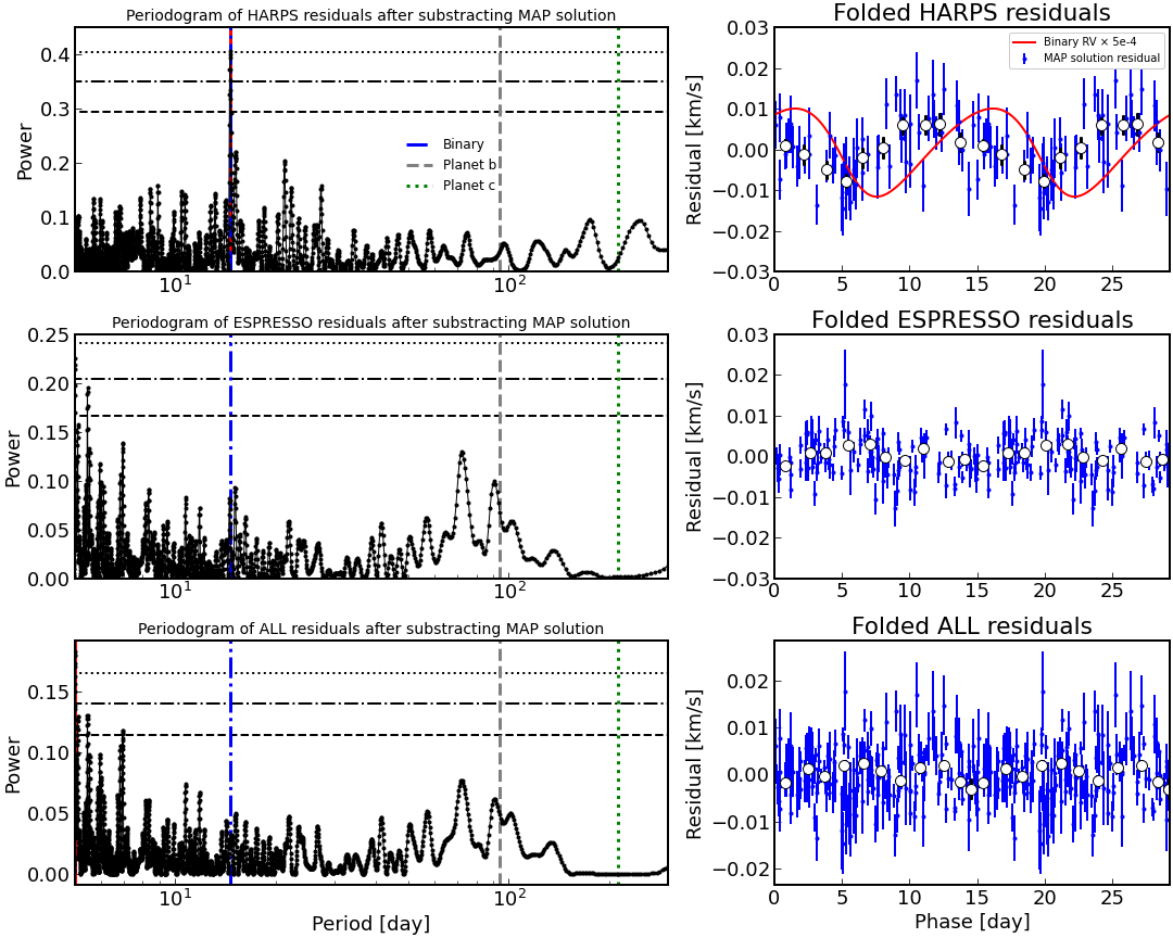
Then we subtract the HARPS and ESPRESSO RV data with the MAP solutions and perform a Generalized-Lomb-Scargle periodogram analysis, shown in Figure 11. We found no peak at binary periodicity when treating HARPS and ESPRESSO data as a whole or ESPRESSO individually, and the peak binary periodicity is present in HARPS data alone, with a false alarm probability around 0.1%. The non-detection of binary periodicity in all RV data is probably due to that the number of ESPRESSO data (103) is much larger than the HARPS data (58).
When we folded the residuals to the binary period, we found a strong modulation in HARPS residuals (top right panel in Figure 11), with a peak-to-peak amplitude of 14 m/s. Compared to the binary RV signal, the residuals excurse the most at the conjunction of the binary, i.e., when the radial velocity is near zero, while in quadrature the excursions are close to zero.
This inconsistency could be the result of secondary star contamination. As noted in Hodzic et al. (2020), when the binary is close to conjunction, the radial velocity of primary and secondary components are close and thus the lines are likely blended together, making the shape of CCF change and impact the derived RV from CCF. When the binary is near quadrature, the RVs of both stars are large enough to prevent the overlap of their line cores, a detailed re-analysis of RV measurements that remove this potential cause is beyond the scope of this paper.
Appendix B Primary/secondary eclipse used in photodynamical modeling